Download Manual

Jana2000
Crystallographic computing system
Václav Petříček & Michal Dušek
Institute of Physics
Academy of Science of the Czech Republic
User manual, part 1
Edited by Michal Dušek, Václav Petříček, Karla Fejfarová & Lukáš Palatinus
Praha 2003
Contents
1
BASIC CONCEPTS.........................................................................................................7
1.1
1.2
1.3
1.4
1.5
1.6
INTRODUCTION................................................................................................................................9
STANDARD STRUCTURE FROM SINGLE CRYSTAL............................................................21
STANDARD STRUCTURE FROM POWDER.............................................................................41
MODULATED STRUCTURE FROM SINGLE CRYSTAL.........................................................55
MODULATED STRUCTURE FROM POWDER .........................................................................89
ADVANCED POWDER REFINEMENT........................................................................................95
REFERENCES .....................................................................................................................105
A
INSTALLATION ...........................................................................................................107
A.1
A.2
A.3
A.4
A.5
B
FTP COMMANDS..........................................................................................................................107
INSTALLATION OF UNIX VERSION.........................................................................................107
INSTALLATION OF WINDOWS VERSION ..............................................................................111
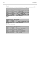
RESULTS OF TESTING REFINEMENTS .................................................................................115
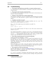
TROUBLESHOOTING..................................................................................................................117
USER PREFERENCES ..............................................................................................121
A.6
A.7
A.8
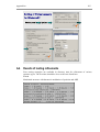
THE CONFIGURATION FILES JANA2000.INI AND JANA2000.HST.................................121
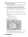
PREFERENCES FOR WINDOWS VERSION...........................................................................121
PREFERENCES FOR UNIX VERSION .....................................................................................122
C
FONT NAMES IN X WINDOWS................................................................................127
D
FORMATS OF FILES USED BY JANA2000..........................................................127
E
WEIGHTING SCHEME ...............................................................................................127
F
GRAPHIC LIBRARIES ...............................................................................................127
G
TABLES FOR PUBLICATION ..................................................................................129
H
HISTORY.......................................................................................................................133
Preface
Jana2000 is a system for solving and refinement of regular, modulated and
composite structures from both single crystal diffraction data and powders. It is
compatible with previous version JANA98 but its functionality is extended.
Jana2000 covers the basic tasks of structure analysis from data reduction and
powder profile analysis to the solution of the phase problem, structure
refinement and presentation of results. The three-dimensional and higherdimensional crystals are treated uniquely in one system regardless of the data
type (single crystal or powder). In addition to regular structure parameters and
their modulation (occupancy, atomic position and harmonic ADP) the system
can also be used for refinement of anharmonic ADP, multipole refinement and
f', f'' refinement. Multiphase refinement is available for both powder and single
crystal data.
This manual consists of three basic parts: The first part (Basic concepts)
introduces Jana2000 with help of several solved examples. In the second part
(Parameters) all structure and profile parameters used in the program are
defined. It also explains the format of parameter files M40 and M41 and the
ways to edit these files. The third part (Structure analysis) describes the whole
process from input of data and solution of the phase problem to structure
refinement and interpretation of results. It describes the basic programs of
Jana2000. The last part (Special topics) contains comprehensive chapter about
transformations and several case studies about work with twins, fivedimensional structures, overlapped reflections, multipole refinement etc.
We hope the book will be useful for both beginners and advanced users and we
welcome any reader's comment.
Václav Petříček
Michal Dušek
Basic concepts
7
1
Basic concepts
This part of the manual is intended as an introduction to Jana2000. It is focused
to practical skills and it skips details and theory. The other chapters will describe
Jana2000 in a more systematic way and they will require some preliminary
experience with the program.
Introduction describes briefly installation, customization, execution and
organization of the program. The details about installation and customization
that are not so frequently needed are described in Appendices. In Introduction
we shall also learn about communication of the principle tools of Jana2000
through the basic files, about naming conventions of atoms etc. Finally, a
complete map of Jana2000 tools is shown with links to related sections of the
manual.
In the next part, we present five solved examples: Standard structure from
single crystal, Standard structure from powder, Modulated structure from single
crystal, Modulated structure from single crystal and Advanced powder
refinement. We describe the complete structure analysis in each example with
special emphasis to utilization of the program tools. The examples are available
in the internet.
After reading Basic concepts, the reader should be able to use Jana2000 for
normal work.
8
Basic concepts
Basic concepts
9
1.1 Introduction
1.1.1 Installation
Jana2000 is freely available on the Jana2000 homepage1 or on the anonymous ftp2
server. The following files can be downloaded:
README.TXT
Downloading and installation notes
jana2000Pack.exe The self extracting installation file for UNIX
jana2000.tar.gz
Installation files for UNIX compressed by gzip
janainst.exe
Files for Windows containing the executable optimized for
Intel Pentium Pro, Pentium II, Pentium III and compatible
processors.3
manual2000.pdf
this manual
manual2000.doc
The recommended way of installation for UNIX is processing of jana2000Pack.exe4
by command
source jana2000Pack.exe
executed from the prompt of csh or tcsh.
For Windows the installation is started by executing janainst.exe.
In both cases, the installation is self-explanatory. Details are given in Appendix A.
1.1.2 Executing Jana2000
The program can be started from the command line, by an icon or through an
associated file type. More sessions of Jana2000 can run together, even in the same
directory, assuming that they are using different job names.
1.1.2.1 Command line syntax
Version for Windows
jana2000 [jobname] [@filename]
Version for UNIX
jana2000 [jobname] [options] [@filename] [&]
Symbol
jobname
@filename
1
Meaning
base name of all permanent files of the structure
Starts Jana2000 in a batch mode without graphical interface using
commands from filename. This option is under development. Please
contact authors if you want to use it.
http://www-xray.fzu.cz/jana/jana.html
ftp://ftp.fzu.cz/pub/cryst
3
Versions for older processors, for instance 486, will be delivered upon request.
4
The extension exe is used in order to convince Web browsers that it is a binary file. In fact the file is not
executable. It is combination of an ASCII header and a binary archive.
2
10
Basic concepts
Options (only for UNIX version)
1
-geometry wxh±x±y Sets window geometry according to conventions for X11 graphics .
Better way of controlling window size is through Preferences (see
later).
Example:
jana2000 my_structure -geometry 500x400+100-50
-scale number
-iconic
-skipini
-dir dirname
-help
&
Jana2000 will automatically fix the ratio between width and height as
it is fixed in the program. It will also change too small or too large
window dimensions.
Sets height of the window as % of the display height.
Starts Jana2000 minimized.
Skips reading of initialisation file.
Sets working directory. Normally JANA2000 starts in the last used
directory.
Lists command line syntax.
(at the end of the command) The program will start in the
background
1.1.2.2 File names
Jobname determines the file names belonging to the calculated structure. They differ
by an extension of three characters, for instance jobname.m50. This convention is
also used in the UNIX version.
Case sensitivity
The file names under Windows are case insensitive, i.e. jobname.m50 is the same as
JobName.M50. Under UNIX, the file names are case sensitive. Thus, we can work
with two different structures jobname and Jobname. The filename extensions must
be always in the lowercase. For instance, the file jobname.M50 will not be
recognized by UNIX version of Jana2000.
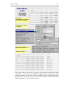
Basic files
The basic files are M50, M40, M95, M94, M91 and SMR for single crystals, M50,
M41, M40, M92 and SMR for powders. They are summarized in the following table.
Basic file
Jobname.m50
Jobname.m40
Jobname.m41
Jobname.m95
Jobname.m94
Jobname.m92
Jobname.m91
Jobname.smr
1
Description
Basic crystal information, options for programs
Parameters of structure model
Profile parameters (powders)
Diffractometer file (single crystals)
Header of M95
Profile data (powders)
Reflections for refinement (single crystals)
Information for creating CIF file
The coordinates following the "-geometry"-option determine the size (in pixels) of the application window and its
position, <x-size>x<y-size><sign><x-position><sign><y-position>. The positions are relative to the left or upper
edges of the screen if <sign> is positive, to the right or lower edges if <sign> is negative.
Basic concepts
11
End-of-line conversion
The ASCII files use special non-printable characters to indicate end of lines. In
Windows it is the ASCII code 10 (LF1) followed by 13 (CR), in UNIX it is the
ASCII code 10 (LF). Jana2000 automatically converts the ends of lines between
UNIX and Windows in the basic files and in most of other imported files2.
Listing files
Name
Jobname.ref
Jobname.fou
Jobname.rre
Jobname.dis
Description
Listing of Refine
Listing of Fourier
Listing of data processing and averaging
Listing of Dist
Temporary files
Jana2000 creates two kinds of temporary files.
•
Files jobname.lnn, where lnn is an extension composed of character l and two
digits, are stored in the current directory. During the regular end3 of Jana2000
they are automatically deleted.
•
Files jcmd*, jm* and *.pcx are saved in the temporary directory. For Windows
version it is JANADIR\TMP, for UNIX it is one of /scratch, /var/tmp, /tmp or
$(HOME). The temporary directory can be redefined by Tools → Preferences.
Jana2000 deletes the temporary files during the regular end. It also scans the
temporary directory for temporary files from improperly terminated runs and if
their number exceeds some limit, it offers their deleting.
Complete overview of files in Jana2000 is in Appendix D.
1.1.3 User preferences
User preferences are set through Tools → Preferences and they are saved to
jana2000.ini. For both versions, they can be used to set size and position of the
Jana2000 window, path to temporary space and external programs. Details are given
in Appendix B.
1
LF is Line Feed; CR is Carriage Return.
Diffractometer files, SHELX files etc.
3
The Regular end occurs when the program is quitted by File → exit. For Windows the Regular end occurs also
when the window is closed by the cross in the title bar. Under UNIX, this is not considered a Regular end
because of difficulties with testing of Destroy event within the program.
2
12
Basic concepts
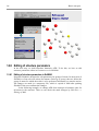
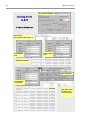
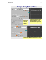
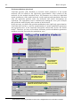
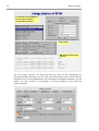
1.1.4 Flowchart of Jana2000
Open/Import
Datred
Editm50
Opens an existing structure in
Jana2000 format or imports a
structure from other formats
(SHELX,CIF).
Converts a diffractometer
file to M94 and M95,
performs data reduction.
Creates or edits M50 with
basic crystal information.
Import rfl. file
Editm50
Imports reduced single crystal
data to M94 and M95. Imports
powder datato M92.
Creates or edits M50 with
basic crystal information.
Create refinement file
Powder parameters
Creates M91 by merging symmetrically equivalent
reflections and by applying extinction rules.
Creates or edit M41 with profile parameters.
Determines which parameters are to be refined.
Refine (profile fitting)
Applies restrictions and refines profile parameters. Makes Le
Bail fit. Input: M41,M50,M92; Output: M41,M80.
Direct methods
Calls SIR97 for single crystals or EXPO for powder.
Input: M91,M50; Output: M40.
Parameters
Creates or edits M40 with structure parameters.
It is convenient for single atoms.
Editm40
Creates or edits M40 with structure parameters. It
is convenient for groups of atoms.
Refine (structure refinement)
Applies restrictions, refines structure and profile parameters. Input: M40 or
M41, M50, M91 or M92; Output: M40 or M41, M80, ref, prf.
Fourier
Contour
Dist
Grapht
Calculates Fourier
maps. Input: M80.
Visualizes Fourier
maps. Input: M81.
Calculates distances
and angles.
Visualizes modulation of
structure parameters
Export
Exports structure to
CIF format.
Transform
Viewer
Makes various transformations: to subgroup,
to superstructure , to another cell etc.
Plots structure in an
external viewer.
The yellow boxes indicate tools that are started through an icon in the basic window of Jana2000. The tools shown
in the white boxes are started through a menu. Only the most important input and output files are shown.
Basic concepts
13
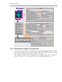
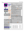
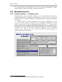
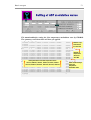
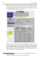
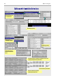
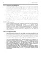
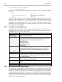
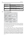
1.1.5 Basic window of Jana2000
Programs of Jana2000 can be executed through their icons in the program basic
window or through the menu Run. The menu Tools lists items that are not classifiable
as a part of some basic program. The menu Parameters can be used for viewing or
setting structure parameters of single atoms. The work with the program starts either
with Datred icon (reading of a diffractometer file) or with File menu (opening of an
existing structure, import of a reduced reflection file).
Tools that are not part of some
basic program.
Open/Close/Edit files.
Import of reflections.
Structure parameters
of single atoms.
The basic programs of Jana2000.
The left double-click starts a
program. The right click starts a
tool for setting run-time program
options if they are available.
The tool for setting run-time
program options for basic
programs of Jana2000. The same
work can be done by rightclicking the relevant program
icon.
Status line
14
Basic concepts
1.1.6 Graphical interface
The graphic user interface supports an intuitive way of work. Its behavior is the same
in UNIX and Windows because the graphical objects are programmed specially for
Jana2000. This makes the program independent of the environment but, on the other
hand, some differences from commonly used conventions occur in Jana2000.
•
TAB changes focus between text boxes. In many cases, it also starts processing of
changes made in the textbox that is just left. For instance, in EditM50, we can
change the space group symbol. After pressing TAB the new symmetry operators
will appear in the relevant text boxes. With new structure, we can also increase
(with help of EditM50) number of dimensions. After pressing TAB new text
boxes appear for definition of q-vector.
•
Ctrl-Y clears the text box under the cursor.
•
ENTER selects button OK. Pressing ENTER twice is equivalent to clicking OK
by mouse.
•
No cut-and paste operations are available.
•
No context menus started by the right mouse button.
•
No sub-windows. Any new "window" is plotted in the basic window and cannot
be moved by mouse.
•
The basic window of Jana2000 can be resized by mouse only in the basic state,
i.e. when no program is running.
•
Ctrl-letter starts programs. For instance, Ctrl-A starts Datred.
•
Alt-letter opens menu. For instance, Alt-T open Tools. In a user forms (for
instance Symmetry in EditM50) Alt-letter selects an item in the form.
•
Letter selects item in a menu. For instance, Alt-T followed by g starts Graphic
viewer.
•
In UNIX version, the Close button of the window manager is ignored by
Jana2000. The Destroy button closes the window but leaves the temporary files
undeleted. For this reason, the UNIX version should be always closed by File →
Exit or by quickly pressing Ctrl-X four times. In Windows, this problem does not
exist.
Basic concepts
15
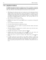
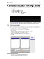
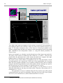
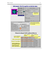
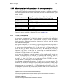
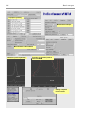
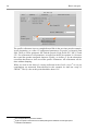
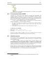
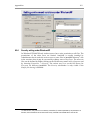
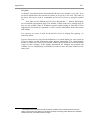
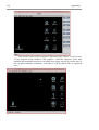
File manager
The File manager of Jana2000 is used for selection of structures or files. In the
mode for selecting structures, it detects Jana files and shows only one name per
structure with a flag STR. For data files, it adds a flag DAT, the remaining files are
listed one-by-one without flags. In the mode for selecting files it lists all files that
correspond to Filter.
In the left panel, double-click on a directory name or ".." changes the directory. The
current version does not support creation of a new directory. In the right panel, the
check button as well as double-click copies the selected file name or a structure to
the text box. OK with a string in the textbox starts the action. If the structure or
filename written in the textbox do not exist they are created - this is especially used
for opening a new structure.
File manager in the mode for selecting structures
File manager in the mode for selecting files
16
Basic concepts
1.1.7 Atom naming conventions
Each atom of the structure model has a name listed in the refinement parameter file
M40. The length of the name is limited to eight characters, but the recommended
length is 5 characters as in some cases Jana2000 appends another characters to the
end of the atom name. The names are case insensitive.
Wildcards
In restric, equation and fixed commands of Refine and the center command of
Fourier groups of atoms can be defined using the wildcards. The wildcards have the
usual meaning:
Sn* denotes all names starting with string “sn” (case insensitive).
S? denotes all names starting with “s” and containing two characters .
?a* denotes names having the letter “a” in the second position.
Molecular positions
If an atom is a part of a molecule, a character denoting the molecular position is
appended to the name. For instance, atom As of a model molecule has name Asa in
the 1st position, Asb in the 2nd one etc.
These extended names can be used for definition of a general plane, in the select
command of Dist etc. They cannot be used in the refinement restriction commands
because they are not explicitly present in the M40 file.
The internal symmetry codes
Some tools of Jana2000 accept the internal symmetry codes indicating symmetry
position of the atom. An internal symmetry code follows immediately the name of an
atom in M40. It takes a symbolic form #sncmtijk , where
#
sn
cm
tijk
separates the internal symmetry code from the atom name.
specifies the |n|th symmetry operator from M50 file. If n is negative, the
operation is combined with the center of symmetry1.
specifies that the mth centering vector will be added to the result of the
symmetry transformation sn (The centering vectors are listed in the
basic crystal information part of any Jana2000 listing)
specifies the additional cell translation defined by three integers i,j,k.
Examples:
Si3#s-3c2t1,-1,0
(Position of Si3 in M40 transformed by the 3rd symmetry operator, by the center of
symmetry, by the 2nd centering vector and by the translation 1,-1,0)
Na1#s2
Cr4#t1,0,-1
An atom name together with an internal symmetry code can exceed the length of 8
characters because it is never present in the m40 file. The internal symmetry codes
can be used in Contour for the definition of the general section plane and in Grapht
for plotting t functions. They are listed in the one-column form2 of the listing of Dist
or by Locator tool of Grapht.
1
2
if it exists in the structure - otherwise an error message occurs
It can be selected in the basic commands for Dist.
Basic concepts
17
1.1.8 Basic steps with Jana2000
In this part we shall describe the basic steps with Jana2000 during typical structure
analysis. It is based on the Flowchart of Jana2000 (§ 1.1.4 ) and on the brief
description of Jana files in § 1.1.2.2 .
Input of data
At the beginning, we need to read diffraction data and input the basic
crystallographic information. Jana2000 offers three ways how to begin.
•
Open/Import (started from the menu File → Structure → Open or File →
Import) works with a previously defined structure.
•
Datred starts from a diffractometer file, performs data reduction and converts the
file to M94 and M95 (the common diffractometer format). Then the basic crystal
information must be defined by EditM50 that yields the file M50.
•
The last possibility (File → Reflection file → Import) is used (1) if no
diffractometer file is available, (2) for powder data and (3) for joining data from
various sources. 1 The imported reflections must be already reduced by other
software or by Datred. This tool is very flexible; it enables transformations
between cells and dimensions and it is explained later in this manual. Like in the
previous example, the imported reflections are converted to the M94 and M95
format.
Determination of symmetry
Jana2000 offers only limited tools for finding proper symmetry. In Datred there is
possibility to calculate the Point group test that reads reflections from M95 and lists
Rint for a given point group symmetry. The systematic absences are listed during
creation of the refinement file M91 (File → Reflection file → Create refinement file)
after entering the tentative (super)space group in EditM50.
Solution of the phase problem
No tools are available for automatic structure determination. However, Jana2000 can
exchange information with SIR97 [1] and EXPO [2] that solve structures by direct
methods. For calling these programs from Jana2000 M50 and M91 files are
necessary. The file M91 contains non-extinct reflections merged by symmetry. The
resulting structure model from direct methods is imported to the file M40.
Another way to solve the phase problem is the classical (non-automatic) heavy atom
method. For calculating Paterson map we need file M80 that is created by program
Refine. Because no structure is available in this stage, we need only M50 and M91
for Refine and we run only zero refinement cycles2. Then we run Fourier and read
the positions of the Patterson peaks in the Fourier listing3. The position of the heavy
atom can be inserted to M40 by EditM40.
Powder profile refinement
In case of powder data, M91 is created by decomposition of the powder profile.
Therefore, the profile refinement must precede the solution of the phase problem.
The menu Parameters → Powder is used for selection of profile parameters and their
1
Typically, twin domains are measured or integrated independently and the data must be joined.
The options for Refine and Fourier are activated by clicking the relevant icon by the right mouse button.
3
The listing viewer is started through Edit/View menu.
2
18
Basic concepts
refinement keys. Refine makes the profile refinement and LeBail decomposition. The
powder profile can be studied with the Profile viewer (menu Tools → Powder).
Structure refinement
For refinement, we need files M40, M50 and M91. M40 contains parameters of the
structure model and refinement keys. With default setting all parameters are refined
that are not restricted by the symmetry with exception of scale parameters, site
occupation and twin volumes that are implicitly fixed.
Refine has many refinement options accessible by clicking the right mouse button.
The results of the refinement are summarized in the screen and the details are printed
to the refinement listing. Before another refinement we usually need to edit the
structure model. This can be done by program EditM40 that supports editing of
parameters for groups of atoms. A tool started through menu Parameters supports
single atom editing.
For powder data, Refine makes Rietveld refinement. The refinement of profile
parameters can be controlled by menu Tools → Powder. In case of more powder
phases another phase is added by Tools → Phases. An important limitation exists in
Jana2000: the structure of the new phase must be known and added in M40 by
EditM40. In other words, combination of the profile refinement and Rietveld
refinement is not possible.
Fourier maps
Fourier maps are calculated by Fourier that reads M80 as an input. The file M80
contains Fourier coefficients and it is prepared by Refine after the last refinement
cycle. With Fourier options, a variety of maps can be calculated. Contour is used for
visualization of two-dimensional sections through Fourier maps. EditM40 can be
used for adding Fourier maxima to M40.
Dist, Grapht, external viewer
Dist calculates distances, best planes and torsion angles. For modulated structures,
the distances are calculated in steps of the internal coordinate t. Grapht is activated
only for modulated structures. It plots various structure parameters as a function of
the internal coordinate t. An external viewer is started by Tools → Graphic viewer. It
can be any plotting program that accepts CIF file as a command line argument. Very
well tested is communication with program Diamond [3].
How to activate Powder option
With powder structure, we first define the basic crystal information in EditM50.
Then the import of the powder experimental profile is possible by File → Reflection
file → Import. As soon as we choose to import powder data, the powder option of
Jana2000 is activated and fixed. The graphic interface does not allow change of a
powder structure back to a single crystal structure and vice versa.
How to activate modulated structure
Modulated structure is activated by setting number of dimensions in the Cell
subwindow of EditM50. Then we can import reflections by File → Reflection file →
Import. After the import of reflections the possibility to change number of
dimensions is disabled. It is activated again if we delete M94 and M95.
Another way is to import a diffractometer file by Datred. Before the import
number of dimensions must be set and for some diffractometers also q vector(s) must
be defined. Some diffractometers allow measurement of satellite reflections with
three real indices. In these cases Datred converts automatically to 4 or more indices.
Basic concepts
19
Transformations
The menu Tools → Transformations offers several types of transformations that will
be discussed later in detail. The simplest case is the cell transformation. The
transformations change M50, M40 and M91. In M94, the transformation matrix is
saved so that M95 is still consistent with the transformed structure. For instance,
creation of the refinement reflection file can be repeated even with the transformed
structure despite the fact M95 is unchanged.
If we change symmetry by EditM50, i.e. without using a transformation tool, the
relevant changes of the structure model and preparation of the refinement reflection
file must be done by the user. EditM40 contains tools for transformation or
expansion of the structure model by symmetry operators or by user-defined matrices.
Absorption correction
Absorption correction is calculated by Datred. The correction factors are saved in
M95 and they are applied when the refinement reflection file M91 is created.
Therefore, the absorption can be repeated or removed. This is useful when the
chemical composition is not completely known at the beginning of the structure
analysis. Absorption correction can be calculated only if M95 has been created from
a diffractometer file by Datred. M95 created by Import does not contain direction
cosines.
Work with twins
The Cell subwindow of EditM50 can be used for setting the number of twin domains
and for definition of the corresponding twin matrices. In the menu Parameters →
Scale/Twin, we can then define volumes of the twin domains and their refinement
keys. If the twinning matrices are composed only of integers, the reflections of twin
domains are completely overlapped. Refine uses the twinning matrices to combine
corresponding reflections during calculation of structure factors.
If reflections of the twin domains are only partially overlapped the twin domains
should be measured or integrated independently using their local orientation
matrices. Then we proceed this way:
•
In Jana2000 we open new structure twin1 and read the diffractometer file of the
first twin domain. We make data reduction and absorption correction, if
applicable,
•
We create twin2 and do the same with data of the second twin domain. In case of
more domains we prepare twin3, twin4 etc. by the same procedure.
•
Finally, we open new structure twin, define the basic crystal information in
EditM50 (including the number of twin domains and their twinning matrices) and
import files M95 of twin1, twin2, twin3 …. as the twin No 1,2,3 …
In the basic refinement option, a threshold can be defined to determine which
reflections are overlapped and which are separated. A similar approach can be used
for joining diffractometer files of the same crystal measured on more diffractometers.
20
Basic concepts
Basic concepts
21
1.2 Standard structure from single crystal
In this chapter, we present solution of a simple organic structure [4] with structural
chemical formula
S
O
COOCH3
COOCH3
and with the basic crystallographic data summarized in this table:
Cell parameters (a,b,c,β)
a=14.963Å, b= 5.083Å, c=20.099Å, β= 104.15º
Radiation:
MoKα
Monochromator angle
6.07º
Space group
P21/n
Chemical formula
S4O20C72H48
The crystal data measured with four-circle diffractometer are available in the Jana
Web page as aro1.zip.1 The archive contains a diffractometer input file aro1.dca.
1.2.1 Starting Jana2000
When executed without command line parameters, Jana2000 starts automatically in
the last used directory and with the last used job name printed in the status bar2. To
open a new job aro1 we have to do the following:
- (optional) Create a directory and copy aro1.dca here.
- Start Jana2000
- Start File manager of Jana2000 by File → Structure → Open
- Use the left panel to skip to the proper directory
- Define the job name in the text box in the right panel
- Press OK
1
2
http://www-xray.fzu.cz/jana/Jana2000/manual/examples/aro1.zip
At this stage, Jana2000 do not open or test any files of the job.
22
Basic concepts
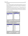
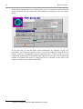
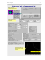
1.2.2 Input of data
At the first step, we start the program Datred in order to read the diffractometer file
aro1.dca. As no M95 exists, Datred opens directly the form for input from
diffractometer. We choose Kuma PD, which is the original name of the Xcalibur
diffractometer, find aro1.dca and press OK. Datred will transfer reflections and the
basic crystallographic information to M94 and M95.
In the next step, we correct the data by Decay and LP correction. Absorption
correction will be omitted since it is negligible for this crystal.
Basic concepts
23
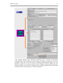
1.2.3 Determination of the space group, solution of the phase
problem
The current version of Datred has no automatic tool for space group determination1.
The Point group test lists Rint for a given point group. In
our example the point group test for the point group 2/m indicates the monoclinic
symmetry. The systematic extinctions can be tested visually in the Reciprocal space
viewer (started from menu Tools). Another possibility is to define a tentative space
grup in EditM50, create the refinement reflection file by File → Reflection file and
view the list of discarded reflections in the Reflection report aro1.rre with help of the
Edit/View menu.
If we save the point group,
cell parameters in M50 will
be rounded accordingly.
1.2.4 Program Editm50
The program EditM50 is used for entering or editing the basic crystallographic
information. It is saved in the file M502.
1.2.4.1 Cell parameters
When started from the diffractometer file the cell parameters are already preset in
EditM50. If the results of the Point group test have been saved, they are already
rounded according to the point symmetry; otherwise they must be rounded by the
user to be consistent with the proposed space group. The e.s.d textbox can be left
clear as the standard deviations of cell parameters are only used for the CIF output
and they are not taken into account in calculation of s.u. of distances3.
1
This is for historical reasons as originally Jana was not intended for ab initio solutions. Various external
programs, for instance XPREP, read hkl file in the SHELX format as input. This can be prepared by Datred →
Export to SHELX.
2
The file M94 contains the original cell parameters read from the diffractometer file. M50 contains the final cell
parameters that are consistent with the structure model and the used symmetry.
3
In future versions of Jana they will be taken into account.
24
Basic concepts
1.2.4.2 Symmetry
The Symmetry form is divided into two parts. The upper part contains the space
group name and the origin shift with respect to the standard choice for the relevant
space group. The lower part contains the symmetry operators, the indicator of the
inversion center at the origin and the cell centering information. Note that in the case
when the inversion center is present but not in the origin, the indicator cannot be
used.
The upper part can be used to define the space group by its symbol and for the origin
specification. The lower part is filled by the derived information whenever the upper
information is filled.
The lower part can be used to define the symmetry explicitly by the symmetry
operators, the cell centering and the presence of the inversion center at the origin.
Any subset of operators which already generates the proper space group is sufficient
as the button Complete the set will generate the rest. Then the program will also try
to derive the symbol and the origin shift with respect to the standard choice. The
procedure for deriving of the space group symbol is successful only if the selection
of the cell is in agreement with the basic rules. All permutations of the cell
parameters are acceptable for triclinic, monoclinic and orthorhombic symmetries.
The higher symmetries except the cubic one should have the dominant axis along c.
Nevertheless all possible settings even those with cannot yield a conventional symbol
are acceptable by the system.
Basic concepts
25
1.2.4.3 Wavelength and atom form factors
In the Radiation subwindow, we can choose or modify the type of radiation and the
wavelength1. In our example, the classical Mo radiation is used. The cathode material
can be defined by the button Targets.
Formula defines chemical composition that is necessary for density calculation and
absorption correction. If we have already done the absorption correction in Datred
the formula field is prefilled. Numbers (including "1") must delimit the chemical
elements, for instance Na2C1O3. The button Fill form factors can be used for
definition of the atom form factors based on the formula. The coefficients are saved
in M50 in the order given in the formula2; i.e. the first atom form factor in M50
corresponds to the first atom in the formula etc. Using of Fill form factors is not the
only way to define atom form factors. They can be also defined independently of the
formula using the last subwindow of Editm50.
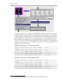
1.2.5 Creating the refinement reflection file
After quitting Editm50, the program offers creation of the refinement reflection file
M913. M91 is created from M95 by applying the corrections defined in M95, by
excluding the systematically extinct reflections and (optionally) by averaging the
reflections according to the symmetry. The limit for observed reflections (see the
flowchart) is only used for printing the import statistics and Rint. The chosen sigma
(Poisson) results from the counting statistics.
The detailed information about systematic extinctions and averaging of reflections is
available in the Reflection report (jobname.rre) accessible by the Edit/View menu.
The information about averaging is important for estimation of data quality and for
approving of the symmetry.
In the scheme below we can see the program discarded the strong reflection -4 0 5.
The corresponding peak in the Profile viewer4 of Datred is shifted from the centre so
that it may be just a tail of some neighboring reflection.
1
The initial values are taken from the diffractometer file.
In M40 file (structure parameters), the atom form factors are referenced to by their sequence number in M50.
Therefore, the order of elements cannot be changed when a structure already exists in M40.
3
It can be also created using the menu File→ Reflection File.
4
The profile viewer is enabled because the input diffractometer file DCA contains diffraction profiles.
2
26
Basic concepts
1.2.6 Solution of the phase problem
1.2.6.1 Solution with SIR97
SIR97 [1] can be called by Jana2000 as an external program by Run → Solution
SIR97. The program is available in http://www.irmec.ba.cnr.it for both Windows
and Unix. The path to SIR97 must be defined in Tools → Preferences.
Jana2000 converts M91 and M50 to the input files jobname.hkl and jobname.sir,
copies the files to the installation directory of SIR97 and starts the program. Then it
waits until SIR97 exits and offers to accept or deny the resulting structure. Finally the
input files of SIR97 are deleted. For successful solution correct definition of the
symmetry and chemical composition is very important.
Starting of SIR97 through Jana2000 is very practical as all conversions (especially
between standard and non-standard space group symmetry) are done automatically.
Some limitations follow from using only very simple set of instructions for SIR97 so
that in difficult cases SIR97 must be run independently1.
1
For this, we can start SIR97 through Jana2000 and copy the input files out of the SIR97 directory to prevent
their deleting. Then we quit SIR97, edit the input file and run SIR97 independently. The resulting ins file can be
imported by File → Import structure.
Basic concepts
27
1.2.6.2 Solution with SHELXS
SHELXS cannot be executed directly from Jana2000 1 . There are two ways to
proceed:
•
We can call Datred → Export to SHELX that transforms M95 to jobname.hkl in
SHELX format. The file jobname.ins must be prepared by the user.
•
If the basic crystal information is defined (i.e. the file M50 exists) we can use
File → Export structure to → SHELX that creates both jobname.hkl and
jobname.ins. The commands specific to SHELXS must be added by hand to
jobname.ins.
In both cases, jobname.hkl contains reflection that are not averaged by symmetry2.
The resulting structure can be imported back to Jana2000 by File → Import
structure from → SHELX.
1.2.6.3 For users that want to skip structure solution
The solution found by SIR97 can also be downloaded from the Web as aro1_sir.zip.3
The archive contains file aro1_sir.m40 that can be imported into the current job by
File → Structure → Copy In command. The tool checks whether the imported files
have a counterpart in the files of the current job. Very often, the files in the current
job without a counterpart should be deleted in order to avoid inconsistencies. In this
1
This function will be added in future versions
If M95 does not exist Jana2000 uses M91 for creation of SHELX hkl file. In such case the reflections are
averaged by the symmetry used for creation of M91.
3
http://www-xray.fzu.cz/jana/Jana2000/manual/examples/aro1_sir.zip
2
28
Basic concepts
case, however, we only want to import M40 and leave the remaining files
unchanged1.
1.2.6.4 Order of atoms returned by direct methods
The order of atoms returned by SIR97 may be different for UNIX and Windows
version and it may depend on processor. The user should compare M40 with the
copy of M40 given in §1.2.6.3 to ensure that the labeling of atoms is the same. We
shall use the labeling further in this chapter.
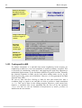
1.2.7 Refinement
The icon of Refine has two functions. The left mouse button starts the refinement; the
right mouse button starts the SetCommands tool for setting refinement options.
1.2.7.1 Refinement options
In Basic commands we set 10 refinement cycles with automatic checking of
convergence (the program will stops when the convergence limit is reached) and
with damping factor one (means no damping). The definition of damping is different
of SHELX: 1 means no damping, 0 means no changes. We use Automatic refinement
keys and Automatic symmetry restrictions. In Select reflections we choose that
unobserved reflections will be used for the refinement. In Weighting scheme we
define the instrument instability 0.02. For the other options, we use their implicit
values. Finally, we click with the left mouse button outside the menu to quit the
SetCommands tool.
1
An easier way would be a simple copy using some external file manager. We use the described way in order to
introduce the Copy In tool.
Basic concepts
29
1.2.7.2 Refinement and viewing of the initial model
As soon as the convergence is reached, Refine shows the refinement results on the
screen. At the same time, it creates refinement listing with detailed information about
the results. The listing is accessible by the Edit/View menu.
The resulting structure can be visualized by an external viewer that is started by
Tools → Graphic viewer. The path to the viewer is defined in Preferences.
30
Basic concepts
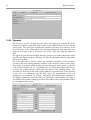
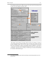
1.2.8 Editing of structure parameters
In the next step, we shall introduce harmonic ADP. To do this, we have to edit
structure parameters either in Parameters or in EditM40.
1.2.8.1 Editing of structure parameters in EditM40
Program EditM40 is designed to edit parameters for groups of atoms. In most tools of
EditM40 we first select an action (for instance Deleting of atoms), then we define the
group of atoms for which the action is to be performed and finally we start the action.
All changes are made in a temporary file, which is copied to M40 after quitting
EditM40 if the user confirms the changes.
In the following example, we change ADP from isotropic to harmonic ones for
all atoms in the structure. Then we can check the made changes by Edit/View →
Editing of M40.
Basic concepts
31
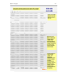
In next two figures, we see how the file M40 looks like before and after the change
of ADP. The first 5 lines in M40 are the header lines; in the first line we see number
of atoms, in the second line there is overall scale factor. The header is followed by
atomic parameters. In this structure every atom has two lines of parameters: Atom
name, chemical type, ADP type, site occupation factor, x,y,z in the first line; U11,
U22, U33, U12, U13, U23 and refinement keys in the second line. For complicated
structures, M40 may take very complex form and it is fully described in the
descriptive part of this manual.
M40 before the change, i.e. with isotropic ADP:
24
0
1.983745
0.000000
0.000000
0.000000
S1
0.012531
O2
0.014128
0
0
0.000000 0.000000 0.000000 0.000000 0.000000
0.000000
0.000000
1 1
0.000000
2 1
0.000000
0.000000
0.000000
1.000000
0.000000
1.000000
0.000000
0.000000
0.000000
0.955264
0.000000
0.972523
0.000000
0.000000
0.000000
0.209162
0.000000
0.314641
0.000000
0.000000
0.000000
0.051917
0.000000
0.249966
0.000000
100000
000000
000000
0111100000
0111100000
M40 after the change, i.e. with harmonic ADP:
24
0
1.983762
0.000000
0.000000
0.000000
S1
0
0
0.000000 0.000000 0.000000 0.000000 0.000000
0.000000 0.000000 0.000000 0.000000 0.000000
0.000000 0.000000 0.000000 0.000000 0.000000
1 2
1.000000 0.955264 0.209162 0.051917
0.012532 0.012532 0.012532 0.000000 0.002881 0.000000
O2
2 2
1.000000 0.972523 0.314640 0.249966
0.014130 0.014130 0.014130 0.000000 0.003248 0.000000
1
100000
000000
000000
1
0111111111
0111111111
The numbers at the end of line are refinement keys. They are briefly explained in §1.2.9 .
32
Basic concepts
1.2.8.2 Editing of structure parameters by Tools → Parameters
In Parameters we first define which atom from M40 is to be edited either by its
sequence number or by selecting from the list that can be opened through the List
button. Then we can select for the atom either Define mode or Edit mode.
In the Define mode we can change chemical type of the atom and type of its ADP1.
Apply site symmetry sets to "0" the refinement keys of parameters that are fixed by
symmetry. In our case it has no influence because the automatic refinement keys are
used, see § 1.2.9 .
In the Edit mode the structure parameters of the given atom and their refinement keys
can be edited individually. Setting of refinement keys has again no influence except
the ai, the site occupation factor, which is never automatic.
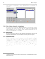
1.2.9 Refinement keys
In the next step, we refine the structure with harmonic ADP. The R-value should
drop down to approximately 5.3%. We can check in M40 which parameters have
been refined.
In our refinement, we use Automatic refinement keys and Automatic symmetry
restrictions (see page 28). This means that the program refines all parameters that are
not fixed by the symmetry. The initial refinement keys in M40 are irrelevant as they
are overwritten by Refine. The exceptions are the scale factors, site occupations and
twin volumes. They are implicitly fixed and they are only refined when the user sets
1
For modulated structures much more possibilities is available.
Basic concepts
33
the corresponding refinement keys to one, for instance by Tools → Parameters.
Refine does not change refinement keys of these parameters.
The automatic options are applicable to almost every structure and their use is highly
recommended.
M40 after the refinement of harmonic ADP.
24
0
1.987328
0.000000
0.000000
0.000000
S1
0.012881
O2
0.013044
0
0
0.000000 0.000000 0.000000 0.000000 0.000000
0.000000
0.000000
1 2
0.015745
2 2
0.019039
0.000000 0.000000
0.000000 0.000000
1.000000 0.955258
0.010095-0.003218
1.000000 0.972560
0.011576-0.005108
0.000000 0.000000
0.000000 0.000000
0.209160 0.051912
0.003884-0.000564
0.314516 0.249963
0.002862-0.002132
100000
000000
000000
0111111111
0111111111
1.2.10 Calculation of Fourier maps
After having the structure refined with harmonic ADP, we can calculate difference
Fourier map and localize hydrogen atoms. Fourier uses the structure factors
calculated by Refine and saved in M80 as an input. Therefore, it is necessary to run at
least zero refinement cycles before starting Fourier.
Like in the case of Refine the left mouse button starts Fourier, while the right mouse
button starts the SetCommands tool for editing of Fourier options. Implicitly, the
program makes Fourier calculation and Peak interpretation using reflections (see
Basic commands), The map is calculated in the independent volume of the
elementary cell in the most convenient orientation with step of 0.25 Å (see Scope of
the map). The program searches for N+5 largest positive maxima, where N is the
number of missing atoms calculated from the formula in M50 1 (see Peaks
commands). The only option the user has to change in our case is the Type of the map
that should be Difference Fourier.
The calculated Fourier map is stored in M81. The Contour program plots the twodimensional sections through the map as contour plots using M81 as an input.
Fourier maxima and minima are stored in M48 and M47, respectively. Detailed
information about Fourier calculation and found peaks is available in the listing of
Fourier.
EditM40 can be used for adding Fourier maxima from M48 to M40. The process of
calculating Fourier and refining new atoms is repeated until all atoms of the structure
are located.
Dist can be used for calculation of distances between atoms and Fourier maxima or
minima. Their inclusion to the calculations is controlled in the Dist options.
1
In M40, there are 24 atoms. The formula previously defined through EditM50 is S1O5C18H12, number of
formula units equals to 4. The number of interpreted difference peaks will be (36-24)+5 = 17.
34
Basic concepts
Basic concepts
35
After localization of all relevant difference maxima, the structure should contain 36
independent atoms in M40 and the resulting R factors should be as shown here:
1.2.11 Structure interpretation
1.2.11.1 Plotting of the structure
We have already shown in § 1.2.7.2 page 29, that the structure can be visualized by
an external plotting program. In this example, we use the plotting program Diamond
[3].
36
Basic concepts
1.2.11.2 Calculation of distances
The distances are calculated by program Dist. For a given atom, the distances and
angles are listed between d(min) and d(max) distances. The limits can be defined
either independently for each chemical type or equally for all stoms. D(max) for
chemical types is implicitly set to 3Å when inserting an atom by EditM40 and it can
be changed through EditM50 in the Atom form factors subwindow. Jana2000 does
not use any kind of tables of atomic radii in the distance calculation.
The maxima and minima from Fourier calculation stored by Fourier in M47
and M48, respectively, can be included into distances calculation. For these
positions, D(max) is always set to 3Å.
In the following example, we first set options for the distance calculation
through the SetCommands tool for Dist. The interface enables selection of central
and surrounding atoms in order to limit the output to requested information. In the
listing shown in the example there is the central atom O4 with coordinated O3, C5,
O6, C15 and C24. The nested lines show angles A1-A2-A3, where A2 is the central
atom printed in the heading (O4 in this case) while A1 and A3 are some another
atoms coordinated to A2; for instance the first angle 68.0º is O3 - O4 - C5, the
second value 95.9º belongs to O3 - O4 - O6 etc.
Besides the listing, there is another output of Dist stored in M61 in one column
format. This listing M61 contains symmetry codes (see § 1.1.7 , page 16).
Basic concepts
37
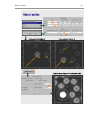
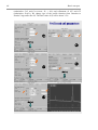
1.2.11.3 Plotting Fourier map with Contour
Fourier maps can be visualized by Contour program. Although plotting of Fourier
map is not necessary for solution of this simple structure, we shall nevertheless give
two basic examples of Contour application. It is a good starting point for § 1.4 where
Contour plots are important for understanding the structure.
In the first example, Contour plots directly sections from M81 pre-calculated by
Fourier. In this file the Fourier map is stored as a sequence of two-dimensional
sections; their orientation and number depends on the Scope options (see page 33). In
our case, the sections are parallel with the ac plane and they are stacked along the b
axis. Contour plots the first section and provides button M+ and M- for moving
forward and back in the sections along b.
38
Basic concepts
Very often, some special orientation of the sections is required. If the orientation is
one of ab, ac or bc it can be defined as Map axis in the Scope options of Fourier, see
page 33. For other orientations, there is the General section tool available in the
Contour program that calculates an arbitrary section through the Fourier map using
M81 calculated in the independent volume, i.e. using the default parameters of
Fourier Scope.
In the next example, we calculate a section through one of the rings in our molecule.
The plane of the section is defined by three atoms S1, C9 and C7. The first two
atoms define the horizontal axis of the section; the third one completes the righthanded system of Cartesian axis with the origin in the first atom.
The Scope1 of the section defines (in angstroms) the size of the horizontal, vertical
and perpendicular axis, respectively. If the size of the perpendicular axis is greater
than zero the program calculates set of equally oriented sections that are stacked
along the direction perpendicular to the section plane with the stacking step equal to
the Interpolation step. In our example, we calculate only one section.
S1 is automatically moved to the centre of the section, i.e. to the point (2.5, 2.5, 0).
With this shift, however, the ring is not fully visible. Therefore, the position of S1 is
redefined to (1.5, 1.5, 0).
The appearance of curves is influenced by the Interpolation step of the general
section and by the step used for calculation of the map (see Step in the Scope options
for Fourier). For smooth curves, both of them should be 0.1Å or less.
1
The Scope of Contour general section is not the Scope for calculation of Fourier map.
Basic concepts
39
C7
S1
C9
S1
C9
40
Basic concepts
1.2.11.4 Creating CIF output
In the last step, we shall create CIF file through File → Export structure to → CIF
for publication purposes or as an input to other programs. The tools of Jana2000
contribute to the file jobname.smr that is used for creation of CIF. If the complete
structure solution from the reading of diffractometer files to the final refinement was
done in the same directory using the same job name, the smr file will contain all
necessary information. Otherwise, before creating CIF some steps must be repeated.
The steps preceding creation of CIF:
•
(If the smr file is not reliable,1 delete it.)
•
Datred: If we start from the point-detector diffractometer file, repeat the Decay
and LP correction. If an absorption correction is used, repeat it using the
definitive cell contents. Then create new file M91.
•
EditM50: check if the estimated standard deviations of cell parameters are
present.
•
Refine: check whether there is the instability coefficient introduced in the
weighting scheme (see Weighting scheme in refinement options, page 28) and run
several cycles of refinement using also unobserved reflections (Select
reflections) with output of Fo-Fc table (Basic commands).
•
Fourier: run zero refinement cycles with unobserved reflections included in the
calculation. (see Select reflections in refinement options). Then calculate the
difference Fourier map using Weighting of reflections (see Basic commands for
Fourier). 2
•
Dist: set carefully options for Dist in order to limit the output to important
distances and angles. Then run Dist. Repeated runs of Dist do not cumulate
information in the smr file. The new run overwrites old distances in smr. As
calculation of all needed distances and angles in one run of Dist is often
impossible, the corresponding section in the CIF needs some user editing.
•
Run File → Export structure to → CIF. If the program has all possible
information the only message shown is
1.2.11.5 Making tables for publication
See Appendix G.
1
2
Possible reason can be changing of job name or using of M50 that is not consistent with M94.
Large number of unveighted weak reflections may generate large extremes in the Fourier map.
Basic concepts
41
1.3 Standard structure from powder
The objective when implementing powders into Jana2000 was creation of a unique
interface for single crystals and powders. The structure determination from powder
data is thus very similar to the work with single crystals. Differences occur mostly at
the initial stage, i.e. during reading of data and profile refinement. The powder option
as initially introduced in the year 2000 is described in [5].
In this chapter, we present solution of a simple powder structure Sr2CeO4 [6] with the
following parameters:
Cell parameters
Radiation
Monochromator
Space group
Chemical formula
Profile data format
Measurement technique
Absorption factor µr
a=6.12Å, b=10.36Å, c=3.59Å
Cu 1.5406Å with α2 component filtered out
26.3º(quartz monochromator , 1 0 1 reflection,
parallel setting)
Pbam
Sr2CeO4, Z=2
MAC
Cylindrical sample (Debye-Scherer)
1.8
The profile data are available in the Jana Web page as sco1.zip.1
1.3.1 Data preparation
Input: profile data, crystallographic information
Output: M50, M92
The cell parameters must be known as Jana2000 does not contain any indexing tool.
1.3.1.1 Entering crystal data by EditM50
In the first step, we prepare M50 by entering cell parameters, space group, radiation
type, wavelength and atom form factors. We proceed exactly like in the case of
single crystal structure, see page 23. Cell parameters, space group and radiation
wavelength are used for generation of Bragg positions. The atom form factors will be
used later in the structure refinement. Special attention should be paid to proper
completion of the Radiation form.
1
http://www-xray.fzu.cz/jana/Jana2000/manual/examples/sco1.zip
42
Basic concepts
1.3.1.2 Reading of profile data
After having completed the basic crystallographic information we can import the
profile data through File → Reflection file → Import file(s) from various sources.
We choose the MAC format. The imported profile data are saved in M92 that plays
the same role like M95 in case of single crystals: it is the common format for
experimental powder data used by Jana2000.
After importing powder data the powder option of Jana2000 is activated while
the options special for single crystals are disabled.
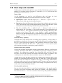
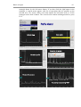
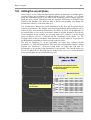
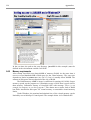
1.3.1.3 Using profile viewer
In Tools we can start Powder → Profile viewer to plot part of the experimental
profile from M92. The buttons on the right are used for navigation through the
profile and for setting of the viewer options. The profile viewer is a rather complex
tool so and here we shall demonstrate only several basic functions.
Buttons X+, X-, Y+ and Y- are used for adjusting the scale in the horizontal (X)
and vertical (Y) direction. Shrink changes both the horizontal and vertical scale to
see the complete plot in the viewer window. Pnts switches between the default view
with visible experimental points and the view where only the polyline connecting the
points is visible. The button "?" starts a help mode that prints a short comment for
each button that is pressed.
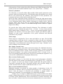
It the next scheme, we first import the profile data and plot the profile. Then
the help mode is demonstrated for the case of button Shrink and the whole profile is
shown as the result of pressing Shrink. We can select an area in the plot using a
Basic concepts
43
rectangle drawn by the left mouse button. If we then click the right button in the
rectangle, a context menu appears with list of operations that are possible on the
selected area. We choose Make zoom that adjusts the horizontal scale to fit the
rectangle in the whole window. The vertical scale remains unchanged until we press
Fit Y.
44
Basic concepts
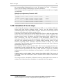
1.3.2 Refinement of profile parameters
Profile parameters are refined by Refine. The output files are M41 (the profile
parameters), M91 (input for EXPO) and M80 (input for Fourier).
1.3.2.1 Le Bail decomposition
Tools → Powder → Make LeBail starts the Le Bail decomposition. The output files
are jobname.prf and jobname.m91. In M91, there are results of the peak
decomposition, i.e. the squares of structure factors and their e.s.d's. The prf file
contains the calculated profile based on profile parameters and Bragg positions. M91
can be used for solution of the phase problem by EXPO (see later) or for calculation
of the Patterson map1.
In this stage, however, the profile parameters have not been yet refined. Implicitly
the only non-zero profile parameter is GW=5, so that the program generates very
narrow peaks based on this parameter. In Tools → Powder → Plot powder profile we
can compare the calculated (prf) and experimental (M92) profile.
hk l mno
0
1
0
2
1
1
0
2
1
2
0
1
2
1
2
2
2
0
2
2
0
0
3
1
2
1
2
2
4
4
0
3
3
1
2
4
0
0
1
0
0
1
1
0
1
0
0
0
1
1
0
1
1
1
0
0
0
0
0
0
0
0
0
0
0
0
0
0
0
0
0
0
0
0
0
0
0
0
0
0
0
0
0
0
0
0
0
0
0
0
0
0
0
0
0
0
0
0
0
0
0
0
0
0
0
0
0
0
I
825.0
823.8
1518.1
5236.9
6546.1
3332.1
3245.9
1504.9
480.1
1008.0
2893.1
1921.2
1034.0
637.8
996.8
1725.9
4116.9
2676.1
s(I)
1.0
1.0
1.0
1.0
1.0
1.0
1.0
1.0
1.0
1.0
1.0
1.0
1.0
1.0
1.0
1.0
1.0
1.0
1
1
1
1
1
1
1
1
1
1
1
1
1
1
1
1
1
1
0
0
0
0
0
0
0
0
0
0
0
0
0
0
0
0
0
0
1
1
1
1
1
1
1
1
1
1
1
1
1
1
1
1
1
1
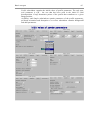
1.3.2.2 Powder parameters
Powder parameters can be edited using Parameters → Powder. This starts a tool
similar to EditM50 that contains all profile parameters. Their values are stored in
M41 that is analogy of M40.
In the following scheme, there are copies of all subwindows of Powder parameters
with their default values. Their refinement keys are all set to zero so that no powder
parameters are refined.
Basic subwindow contains information about radiation. The numbers edited here are
saved not only in M41 but also in M50 so that the changes are reflected in Radiation
subwindow of EditM50. Conversely, the changes made in the Radiation subwindow
of EditM50 will be also visible in the Basic subwindow of Powder parameters. The
same rule holds for the Cell subwindow of Powder parameters that corresponds to
the Cell subwindow of EditM50.
1
Fourier requires the file m80 as an input. Calculation of Patterson map is the only case when M80 can be
replaced by M91.
Basic concepts
45
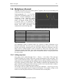
Profile subwindow contains the initial values of profile parameters. The only nonzero parameter is GW - the one that has been used in the initial Le Bail
decomposition. Cutoff determines points of the profile that contribute to a given
Bragg position.
Asymmetry and Sample subwindows contain parameters of the profile asymmetry,
preferred orientation and absorption. Corrections subwindow contains background
and shift parameters.
46
Basic concepts
1.3.2.3 Refinement options
Prior to the refinement of the profile parameters Refine executes the Le Bail
decomposition in order to extract intensities that are necessary for the calculation1.
Then it refines the profile parameters using the extracted intensities in one or more
refinement cycles. The number of refinement cycles between two consecutive Le
Bail decompositions is an important parameter. If it is one (i.e. the Le Bail
decomposition is executed prior to each refinement cycle) it may cause instability of
the refinement. On the other hand, too large number slows down the refinement and
must be coordinated with number of refinement cycles to avoid false convergence
(see later). We recommend setting the frequency of Le Bail decomposition to one
and change it only if the refinement is unstable.
The Basic commands subwindow of the refinement options looks similarly like in
case of single crystal refinement except two points: Frequency of Le Bail
decomposition and Apply Berar's correction.
Frequency of Le Bail decomposition must be less than Number of cycles and Number
of consecutive cycles used in Check for convergence. This is because the refinement
may completely converge before a new Le Bail decomposition is calculated.
Berar's correction is estimated during the refinement and it is applied to standard
uncertainties of all refined parameters (profile, elementary cell and structure).
Usually it leads to larger values that are more realistic. The correction does not
influence the refinement itself.
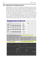
1.3.2.4 Refinement of background parameters
Background parameters should be refined first. The background is usually modeled
by Legendre polynomials using from 5 to 15 terms. Here we shall refine 15 terms.
No initial values of the terms are necessary. Their refinement keys must be set to "1"
using Edit backlground in Powder options → Corrections. After the refinement, the
Rp factor will drop to approximately 13%. Then we can visualize the new calculated
profile by Profile viewer.2
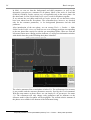
In the following scheme, we can see the sharp peaks generated by GW = 5 are
now shifted onto the refined background. Usually this is a good starting point for
1
If there is already a structure available, the intensities are calculated from the structure. At the end, Refine
makes the peak decomposition and creates M80 for calculation of Fourier maps. For compatibility with some
tools, it also creates M91.
2
The prf file with calculated profile is only created when Refine finishes regularly. With Refine interrupted by
Cancel button, no prf file is created and Profile viewer plots only the experimental profile from M92.
Basic concepts
47
refinement of profile parameters. In some special cases it may be better to find more
favorable starting point by changing GW with Parameters → Powder → Profile,
calculating Le Bail decomposition through Tools → Powder → Make Le Bail and
inspecting the resulting profile with Profile wiever. In the scheme below we show a
plot of the calculated profile for GW = 100.
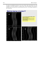
1.3.2.5 Refinement of profile, cell and shift parameters
In the next step, we refine the parameter GW. The refinement should converge to Rp
about 7%. Then we proceed with refinement of cell parameters and zero shift
48
Basic concepts
(subwindow Cell and Corrections, Rp ≈ 4%) and refinement of GU and GV
(subwindow Profile). We change type of the profile function from Gaussian to
Pseudo-Voigt and refine LX. The final value of Rp will be about 3.5%.
c
d
e
f
d
Basic concepts
49
1.3.3 Refinement of structure
1.3.3.1 Solution of the structure by EXPO
EXPO [2] performs the extraction of the structure factor amplitudes from the powder
pattern by using the Le Bail algorithm. The extracted integrated intensities are
processed by Direct Methods in order to solve the structure. Jana2000 starts EXPO
as an external program that must be downloaded and installed separately by the user.
The path to EXPO must be defined in Tools → Preferences. EXPO is used in a mode
that skips the profile decomposition and uses the intensities extracted by Jana2000.1
EXPO can be called through Run menu. Jana2000 saves extracted intensities to
EXPO input file jobname.rfl and prepares the crystallographic information and EXPO
control commands 2 in jobname.exp. Both input files are created in the directory
where EXPO is installed. Then Jana2000 starts EXPO and waits until the external
program exits. After confirmation, Jana2000 reads the results and deletes input files.
The advantage of starting EXPO through Jana2000 is that all conversions between
EXPO and Jana2000 are done automatically. As EXPO accepts only standard space
groups Jana2000 converts some non-standard groups before starting EXPO and
transforms the results back to the original setting. The disadvantage is that Jana2000
uses only very simple set of instructions for EXPO. However, it is sufficient for most
cases as EXPO is designed for fully automatic run.
1.3.3.2 For users that want to skip structure solution
The solution that would be created by EXPO can also be downloaded as
3
sco1_expo.zip. The archive contains file sco1_expo.m40 that can be imported into
the current job by File → Structure → Copy In command (see also page 27).
1.3.3.3 Structure refinement
In the next step, we shall refine the structure model created by EXPO. Unlike in the
profile refinement there is no option for frequency of Le Bail decomposition because
the intensities are now calculated from the structure model. The Le Bail
decomposition is only activated when Make only profile matching is used.
In the refinement, we do not fix any previously refined profile parameter; they
should be refined together with structure parameters. After the refinement, we shall
see relatively good agreement factors but the isotropic ADP's will be very small or
negative. This is caused by missing absorption correction.
Finally, we can try whether refinement of harmonic ADP is reasonable. The
refinement yields acceptable harmonic parameters for Sr1 Ce1 and O2 but for O1
they are not positive definite.
In the later stage of the refinement, we can enable Apply Berar's correction to get
more realistic standard uncertainties in the distances calculation.4
1
In the future export of the powder profile to EXPO will be also possible.
With the commands prepared by Jana2000 EXPO skips extraction of intensities (i.e. the EXTRA program) and
uses the intensities supplied by Jana2000.
3
http://www-xray.fzu.cz/jana/Jana2000/manual/examples/sco1_expo.zip
4
Application of this correction at the beginning of the refinement could bias the automatic recognition of large
changes of the scale factor that should lead to repeating of the refinement cycle with new scale without changing
the other parameters.
2
50
Basic concepts
4
0
0
0.205928 0.000000
0.000000
0.000000 0.000000
0.000000 0.000000
Ce1
2 1
-0.000825 0.000000
Sr1
1 1
0.001073 0.000000
O1
3 1
-0.001956 0.000000
O2
3 1
0.009627 0.000000
0
0.000000 0.000000 0.000000 0.000000
4
0
0
0.835478 0.000000
0.000000
0.000000 0.000000
0.000000 0.000000
Ce1
2 1
0.019607 0.000000
Sr1
1 1
0.021845 0.000000
O1
3 1
0.019616 0.000000
O2
3 1
0.033073 0.000000
0
0.000000 0.000000 0.000000 0.000000
0.000000 0.000000 0.000000 0.000000
0.000000 0.000000 0.000000 0.000000
0.250000 0.000000 0.000000 0.000000
0.000000 0.000000 0.000000 0.000000
0.500000-0.063179-0.320225-0.500000
0.000000 0.000000 0.000000 0.000000
0.500000 0.143546-0.193567 0.000000
0.000000 0.000000 0.000000 0.000000
0.500000-0.225932-0.045928-0.500000
0.000000 0.000000 0.000000 0.000000
0.000000 0.000000 0.000000 0.000000
0.000000 0.000000 0.000000 0.000000
0.250000 0.000000 0.000000 0.000000
0.000000 0.000000 0.000000 0.000000
0.500000-0.063340-0.320221-0.500000
0.000000 0.000000 0.000000 0.000000
0.500000 0.143255-0.193322 0.000000
0.000000 0.000000 0.000000 0.000000
0.500000-0.225864-0.046377-0.500000
0.000000 0.000000 0.000000 0.000000
Basic concepts
51
1.3.4 Multiphase refinement
Jana2000 can refine up to five powder phases1 together. Here we present adding and
refinement of the second phase.
In the paragraphs 1.3.1 - 1.3.3 we have
refined the dominating phase in sco1,
Sr2CeO4. Careful examination of the
calculated versus observed profile
reveals there are small undescribed
peaks, for instance around 42º2θ. This
is because there is an admixture of
SrCeO3 in the sample with crystal data
known from other experiments and
summarized in the following table.
Cell parameters
Space group
Chemical formula
Structure
Ce
Sr
O1
O2
a=6.148Å, b=8.586Å, c=6.010Å, α=β=γ=90º
Pnma
SrCeO3, Z=4
0.000000
0.063373
0.857028
0.225611
0.000000
0.679763
0.805629
0.955184
0.000000
0.500000
0.000000
0.500000
Important limitation
The multiphase option is possible either for a profile (Le Bail) refinement or for
Rietveld refinement. The two types of refinement cannot be mixed. If we refine
powder and structure parameters of the first phase (Rietveld refinement), the new
phase must be added together with its structure to allow the same type of the
refinement. On the other hand, if we refine only powder parameters of the first phase
(Le Bail refinement), the new phase must be identified only by cell parameters and
the space group.
1.3.4.1 Adding new phase
New phase can be added through Tools → Phases → New Phase. This starts the
EditM50 dialogue for setting of the basic crystal information for the new phase. The
Phase textbox should contain a short (eight characters) phase identifier. In Radiation
subwindow, the wavelength and the radiation type are already defined as they have
been taken from the previous phase. After finishing of EditM50 the thumbnails with
phase identifiers will appear in the left lower corner of the Jana2000 basic window.
They can be used for switching between phases.
We switch to the new phase and enter its structure (EditM40 → Replacing/inserting
atoms). The atom names must be unique for all phases. For instance, if there is an
atom S1 in the first phase this name is not allowed in the second phase.
1
This limit can be changed during program compilation.
52
Basic concepts
As soon as the new phase is added the basic files M40, M41 and M50 acquire
multiphase organization with separate data sections for both phases.
M40 after adding the new phase
This is volume fraction
4
0
0
4
0
0
0.843921 0.000000
0.000000
0.000000 0.000000
0.000000 0.000000
Ce1
2 1
0.019607 0.000000
Sr1
1 1
0.021847 0.000000
O1
3 1
0.019617 0.000000
O2
3 1
0.033078 0.000000
Ce_b
2 1
0.037995 0.000000
Sr_b
1 1
0.037995 0.000000
O1_b
3 1
0.037995 0.000000
O2_b
3 1
0.037995 0.000000
of the new phase
0
0
0.000000 0.000000 0.000000 0.010000
100000
0.000000 0.000000 0.000000 0.000000
0.000000 0.000000 0.000000 0.000000
0.250000 0.000000 0.000000 0.000000
0.000000 0.000000 0.000000 0.000000
0.500000-0.063340-0.320221-0.500000
0.000000 0.000000 0.000000 0.000000
0.500000 0.143255-0.193323 0.000000
0.000000 0.000000 0.000000 0.000000
0.500000-0.225863-0.046377-0.500000
0.000000 0.000000 0.000000 0.000000
0.500000 0.000000 0.000000 0.000000
0.000000 0.000000 0.000000 0.000000
1.000000 0.063373 0.679763 0.500000
0.000000 0.000000 0.000000 0.000000
1.000000 0.857028 0.694371 0.000000
0.000000 0.000000 0.000000 0.000000
1.000000 0.725611 0.544816 0.000000
0.000000 0.000000 0.000000 0.000000
000000
000000
0000100000
0110100000
0110100000
0110100000
0000000000
0000000000
0000000000
0000000000
Basic concepts
53
M41 after adding the new phase
bckgtype 1 bckgnum 15 manbckg 0 wtlebail 1
absor 1 mir 1.8
phase Phase#1
proffun 3 asymm 0 strain 0 cutoff 8
phase SrCeO3
proffun 3 asymm 0 strain 0 cutoff 8
end
**************************************************************************
# Shift parameters - zero, sycos, sysin
0.323450 0.000000 0.000000
100
# Background parameters
407.3499-268.6363 312.9955-104.7968-27.48167 61.88438
111111
-47.05416-7.195762 39.71324-30.45667 19.92561 3.898507
111111
-13.68987 1.227813-4.748011
111
### phase Phase#1
# Cell parameters - a,b,c,alpha,beta,gamma
6.120009 10.35531 3.596630 90.00000 90.00000 90.00000
111000
# Gaussian parameters - U,V,W,P
39.10152-20.71844 32.72264 0.000000
1110
# Lorentzian parameters - X,Xe/Xs,Y,Ye
2.630812 0.000000 0.000000 0.000000
1000
### phase #2SrCeO3
# Cell parameters - a,b,c,alpha,beta,gamma
6.148000 8.586000 6.010000 90.00000 90.00000 90.00000
000000
# Gaussian parameters - U,V,W,P
39.10152-20.71844 32.72264 0.000000
0000
# Lorentzian parameters - X,Xe/Xs,Y,Ye
2.630812 0.000000 0.000000 0.000000
0000
M50 after adding the new phase
title
lambda 1.5406 radtype 1 lpfactor 1 monangle 0.806
datcolltemp 293
-----------------------------------------------------------phase Phase#1
cell 6.120009 10.35531 3.59663 90 90 90
esdcell 0 0 0 0 0 0
spgroup Pbam 55 3
centro
lattice P
symmetry x y z
symmetry x y -z
symmetry 1/2-x 1/2+y z
symmetry 1/2-x 1/2+y -z
unitsnumb 4
chemform Sr2Ce1O4
atom Sr
atweight 87.62 atradius 3
f' -0.3528 f" 1.82
formtab -56
38.0000 37.9460 37.7860 37.5320 37.1970 36.8020 36.3630
. . . .
-----------------------------------------------------------phase #2SrCeO3
cell 6.148 8.586 6.01 90 90 90
esdcell 0 0 0 0 0 0
spgroup Pnma 62 3
centro
lattice P
symmetry x y z
symmetry 1/2+x y 1/2-z
symmetry 1/2-x 1/2+y 1/2+z
symmetry -x 1/2+y -z
unitsnumb 4
chemform Sr1Ce1O3
atom Sr
atweight 87.62 atradius 3
f' -0.3396 f" 1.8517
formtab -56
38.0000 37.9460 37.7860 37.5320 37.1970 36.8020 36.3630
. . . .
35.8970
35.8970
54
Basic concepts
In M41, we can see that the background and shift parameters as well as the
absorption correction are common for all phases. Most of the tools of Jana2000
(Editm40, EditM50, Powder options etc.) are applicable only to the active phase. On
the other hand, Le Bail, Refine and Profile viewer work for all phases together.
If we activate the new phase and look at Powder options we see that their values
have been taken from the first phase1. The refinement keys, however, are checked
only for the common parameters, i.e. for background parameters and the shift
parameter.
After introduction of the new phase, we can execute Tools → Powder → Make
LeBail. In the Profile viewer we shall see new row of Bragg positions corresponding
to the new phase that exactly fits with the yet unexplained peaks. When we click the
left mouse button near a Bragg position indicator, we will get an information window
with details about the peaks including their phase identifier.
The relative amount of the second phase is below 2%. The refinement of its structure
is not possible and the structure parameters must be fixed by the Fixed command.
With the atom names as shown above we can simply fix All parameters for atoms
*_b. The refinement will only change scale parameters and its influence to the
structure model of the first phase will be negligible. The refined relative amounts of
the phases are available in the bottom of the refinement listing.
1
The powder parameters can be copied between phases by Tools → Powder → Reset powder parameters.
Basic concepts
55
1.4 Modulated structure from single crystal
In this chapter, we present solution of the incommensurate phase of anhydrous
sodium carbonate, Na2CO3 [7]. Its basic crystallographic data are summarized in the
following table:
Cell parameters (a,b,c,β)
Radiation:
Monochromator angle
Space group of the basic structure
q vector
Superspace group
Chemical formula
a=8.920Å, b= 5.245Å, c=6.050Å, β= 101.35º
MoKα
6.07º
C2/m
(0.182,0.000,0.322)
C2/m(α0γ)0s
Na2CO3
The structure was measured using KUMA diffractometer with CCD detector. The
reduced diffractometer data containing satellites up to the forth order are available in
the WWW page of Jana2000 as naco1.zip.1
1.4.1 Reading of data
Although Jana2000 can read directly the integrated data from KUMA, 2 we shall
demonstrate several ways of reading data of a modulated structure.
1.4.1.1 Reading the diffractometer data with four integer indices
The most natural way is to import directly data produced by the diffractometer
software. In our case, it is naco1.hkl file created by KUMA/Xcalibur integration
software and its counterpart naco1.sum with the basic crystal information. The
integration was performed using four indices and the q vector is available in the sum
file. The data in naco1.hkl have been already corrected for LP factors but not for
absorption. This could be done by Jana2000 using the direction cosines recorded to
the file but the absorption is negligible in our case.
1
2
http://www-xray.fzu.cz/jana/Jana2000/manual/examples/naco1.zip
Currently Xcalibur
56
Basic concepts
In the same program Datred we run the Point group test. It not only verifies the point
group symmetry but also rounds the celll parameters according to the saved point
group.
In the next step, we edit the basic crystal information by EditM50. In the Cell
subwindow, the Dimension option is set to four and it cannot be changed, as any
change would be incompatible with the imported data 1 . Values of the q vector
components indicate that an incommensurate approach can be used. The formula and
number of formula units must be entered as close as possible to the correct cell
content in order to get a solution from SIR97.
1
Dimension can only be changed when M94 and M95 files do not exist.
Basic concepts
57
After quitting EditM50 the refinement reflection file is created by discarding
systematically extinct reflections and averaging reflections according to the given
symmetry. Since the CCD data suffer by deeply underestimated sigmas we use
Maximum option in Averaging parameters that compares sigmas resulting from the
Poisson statistics and the ones resulting from averaging symmetrically equivalent
reflections and uses the larger ones for the refinement.
58
Basic concepts
The program discards several strong reflections. Normally, this would indicate an
incorrect symmetry but in our case, this is caused by a weak admixture of another
domain of Na2CO3 in the sample. The integration of CCD data is combined with
local peak hunting in the predicted peak position that may cause a skip from an
extinct diffraction spot of the first domain to a non-extinct peak of the second
domain.
1.4.1.2 Reading reflection file with four integer indices
Very often, the input is not a diffractometer file supported by Datred but a reflection
file processed by some data reduction program. In this paragraph, we shall use as an
input a reflection file containing reduced and corrected diffraction data indexed with
four indices. There is no information available in the file about direction cosines and
orientation matrix. Such data can be imported by File →Reflection file →Import
file(s) from various sources.
In the first step, we create a new job name1 by File → Open and define the basic
crystal information by EditM50. The dimension must be 4, the q vector, super space
group, radiation, chemical composition and atomic form factors are the same like in
§ 1.4.1.1 . Then we start File →Reflection file →Import file(s) from various sources
and select the filename 4indices.hkl (it is available in naco1.zip. 2 ). We define its
format and number of indices in the Specify input reflection file form. The format
specification follows the conventions of FORTRAN programming language. Note
that in our case number of indices is compatible with the dimension defined in
EditM50.
1
In the current job, the import of the reflection file is disabled, as data from diffractometer file are already
present. These two kinds of input cannot be combined. Another way to enable the import tool is to create a new
job name by File → Structure → Open and import M40, M50 but not the other basic files by File → Structure →
Copy in tool.
2
http://www-xray.fzu.cz/jana/Jana2000/manual/examples/naco1.zip
Basic concepts
59
In the scheme below it is also shown that the import tool is not available if some data
have been already imported by Datred because a diffractometer file cannot be
combined with imported files.
After successful import of data we create the refinement reflection file M91 and
continue with solution of the average structure (see § 1.4.2 ).
(Import tool is not available if data have been
already processed by Datred)
“General file” means the format will
be defined using FORTRAN conventions. Free format (*) can be
used if all data are separated by one
or more spaces (also the last index
and intensity!!). In our case “SHELX
on I” would be possible, too.
This summary should be the
same like when importing the
diffractometer file, see § 1.4.1.1
1.4.1.3 Reading reflection file with 3 real indices
In this example we suppose the same situation like in § 1.4.1.2 but we shall import
reflection file indexed with three real indices (3indices.hkl available in naco1.zip.1).
In this case, the import tool transforms the real indices to integer indices using
information about number of dimensions and value of the q vector defined in
EditM50. The Accuracy text box defines tolerance for the values of the real indices
that do not correspond exactly to the values of the q vector components. The
Supercell and Transform indices options enable various transformations of imported
data that will be discussed elsewhere. Unlike the reading of four indices, the program
1
http://www-xray.fzu.cz/jana/Jana2000/manual/examples/naco1.zip
60
Basic concepts
also uses the superspace symmetry to detect systematic extinctions. The extinct
reflections are therefore discarded already during the import and not as usually
during creation of M91.
This summary should be the
same like when importing the
diffractometer file, see § 1.4.1.1
1.4.2 Average structure
1.4.2.1 Solution by direct methods
Sodium carbonate is strongly modulated and its structure determination from only
main reflections is far from reality. Nevertheless, the average structure can be solved
by SIR97 if we use as an input main reflections combined with satellites. The first
structure model returned by SIR97 can be used for refinement of average structure
although its R-value of 26% value is reported by SIR97 as unsatisfactory1.
In the next step, we shall refine the structure model from SIR97. In the refinement
commands we choose only main reflections for calculation, set the instability factor
to 0.02, number of refinement cycles to 100 and automatic checking of convergence.
1
Windows users should use SIR97 with care as it crashes during refinement of the second model. There is a
small time delay when SIR97 reports unsatisfactory R value of the first model and asks whether to continue. The
user must answer “No” during this delay. Otherwise SIR97 will proceed with another model and crash. This does
not occur with UNIX version.
Basic concepts
61
The refinement with isotropic ADP converges to R-value about 50% that drops down
to about 22% after change to harmonic ADP.
The structure must contain CO3 group with the typical C-O distances. It helps to
verify with program Dist whether chemical types of carbon and oxygen have been
properly assigned by SIR97. In our case, they have been interchanged1. The chemical
types can be redefined by editing corresponding numbers in M40 or by Parameters
→Atoms tool (see below). New refinement converges to R value 12%. At the end, we
run EditM40 →Rename atoms according to chemical types to ensure the atom labels
are consistent with chemical types.
1
It may depend on the operating system. SIR97 under UNIX gives sometimes slightly different solution of the
Windows version.
62
Basic concepts
Distances calculated by
Dist indicate incorrect
assignment of chemical
types
Change of chemical type
of O4 from “oxygen” to
“carbon”.
Refinement
results after
correction of
chemical types
EditM40 renames atoms after
the change of
chemical types
1.4.2.2 Creating motifs in M40
For further calculation, it is advisable that atoms neighboring in the structure are
neighboring in M40, too, even if no translation or rotation symmetry is applied. This
is necessary for introducing "molecules" and applying the rigid body approach to
modulation displacements. It also facilitates definition of general sections. Normally
the chemical fragments in M40 can be built when adding atoms one by by the
Replacing/Inserting atoms tool of EditM40.. However, it is not guaranteed for M40
imported from SIR97.
We can see from Edit/View→Editing of M40 file that some atoms have their z
coordinate larger or equal to one and that we need to perform a simple translation
x,y,-1+z. This can be done in the editing program. Moreover, some atoms have
negative x coordinate that can be translated into the first cell by the operation
1+x,y,z. For this, we can use EditM40→Transformation of atomic positions as
indicated in the next scheme.
Basic concepts
63
6
0
0
14.05362 0.000000
0.000000
0.000000 0.000000
0.000000 0.000000
Na1
1 2
0.018117 0.088773
Na2
1 2
0.016378 0.075904
Na3
1 2
Original M40:
0.020384 0.111419
The coordinates in bold should C1
2 2
0.009047 0.078580
be translated to the first cell.
O1
3 2
0.015823 0.035220
O2
3 2
0.084439 0.138996
Transformation of negative
x coordinates:
0
0.000000 0.000000 0.000000 0.000000
0.000000 0.000000
0.000000 0.000000
0.250000 0.000000
0.016176 0.000000
0.250000 0.000000
0.016003 0.000000
0.500000-0.328990
0.029666 0.000000
0.500000 0.335908
0.009242 0.000000
0.500000-0.211082
0.025142 0.000000
1.000000-0.102410
0.066159 0.080114
0.000000
0.000000
0.000000
0.007018
0.000000
0.006151
0.000000
0.008427
0.000000
0.001293
0.000000
0.011611
0.288979
0.053759
0.000000
0.000000
0.500000
0.000000
1.000000
0.000000
0.748563
0.000000
0.750838
0.000000
1.176573
0.000000
0.714059
0.042174
We can check with Refine that the
transformation is correct.
M40 after translations:
6
0
0
14.05363 0.000000
0.000000
0.000000 0.000000
0.000000 0.000000
Na1
1 2
0.018117 0.088773
Na2
1 2
0.016378 0.075903
Na3
1 2
0.020384 0.111418
C1
2 2
0.009047 0.078579
O1
3 2
0.015823 0.035220
O2
3 2
0.084438 0.138994
0
0.000000 0.000000 0.000000 0.000000
100000
0.000000
0.000000
0.250000
0.016176
0.250000
0.016004
0.500000
0.029666
0.500000
0.009242
0.500000
0.025141
1.000000
0.066159
000000
000000
000 0 0
0000111010
000 0 0
0000111010
000 0 0
0101111010
000 0 0
0101111010
000 0 0
0101111010
000 0 0
0111111111
0.000000
0.000000
0.000000
0.000000
0.000000
0.000000
0.671010
0.000000
0.335908
0.000000
0.788918
0.000000
0.897590
0.080112
0.000000
0.000000
0.000000
0.007018
0.000000
0.006151
0.000000
0.008427
0.000000
0.001293
0.000000
0.011611
0.288979
0.053758
0.000000
0.000000
0.500000
0.000000
0.000000
0.000000
0.748563
0.000000
0.750837
0.000000
0.176573
0.000000
0.714059
0.042173
0
0
0
0
0
0
The oxygen atoms are part of the CO3 group are they should be transformed to make
a motif. We can use Dist to check which atoms should be transformed and by which
symmetry operators. At this point we must emphasize that the transformation made
by EditM40→Transformation of atomic positions transforms all atomic parameters
(ADP, modulation, etc.) of the selected atoms.
64
Basic concepts
DIST – Basic commands
Output of Dist:
(For symmetry codes see §1.1.7 )
Transformation
of O2
Transformation
of O1
Resulting coordinates:
C1
0.009047
O1
0.015823
O2
0.084438
2 2
0.078579
3 2
0.035220
3 2
0.138994
0.500000
0.009242
0.500000
0.025141
1.000000
0.066159
0.335908 0.000000
0.000000 0.001293
0.211082 0.000000
0.000000 0.011611
0.397590-0.211021
0.080112 0.053758
0.750837
0.000000
0.823427
0.000000
0.714059
0.042173
Check by Refine
Transformation
of C1,O1,O2:
6
0
0
14.05363 0.000000
0.000000
0.000000 0.000000
0.000000 0.000000
Na1
1 2
0.018117 0.088773
Na2
1 2
0.016378 0.075903
Na3
1 2
0.020384 0.111418
C1
2 2
0.009047 0.078579
O1
3 2
0.015823 0.035220
O2
3 2
0.084438 0.138994
0
M40
0.000000 0.000000 0.000000 Final
0.000000
0.000000
0.000000
0.250000
0.016176
0.250000
0.016004
0.500000
0.029666
0.500000
0.009242
0.500000
0.025141
1.000000
0.066159
0.000000
0.000000
0.000000
0.000000
0.000000
0.000000
0.671010
0.000000
0.835908
0.000000
0.711082
0.000000
0.897590
0.080112
0.000000
0.000000
0.000000
0.007018
0.000000
0.006151
0.000000
0.008427
0.500000
0.001293
0.500000
0.011611
0.288979
0.053758
0.000000
0.000000
0.500000
0.000000
0.000000
0.000000
0.748563
0.000000
0.750837
0.000000
0.823427
0.000000
0.714059
0.042173
New output of Dist:
All atoms of CO3
are in the first cell
Basic concepts
65
The final M40 can be downloaded from the server as naco1_average.zip1. Further
in this chapter we shall use labeling consistent with this file.
1.4.3 Modulated structure
1.4.3.1 Position modulation – 1st modulation wave
With having the average structure finished, we can start refinement of position
modulation parameters. Although the modulations in Na2CO3 are very large, the
refinement can be started from arbitrary small displacements assigned automatically
by Editm40.
With EditM40 we enable refinement of one position modulation wave for
every atom of the structure. EditM40 sets the modulation parameters to small
positive values and it sets the corresponding refinement keys to “1”. These keys are
set irrespective of the symmetry restrictions following from the site symmetry. The
symmetry restrictions are taken into the account by Refine if “Automatic symmetry
restrictions” are used in the basic refinement commands. If the “Automatic
refinement keys” option is also active, Refine will refine as many parameters as
possible with the given symmetry.
1
http://www-xray.fzu.cz/jana/Jana2000/manual/examples/naco1_average.zip
66
Basic concepts
M40 after setting the first position modulation wave by EditM40. The symmetry
restrictions have not been yet applied.
6
0
0
0
13.64836 0.000000 0.000000 0.000000 0.000000
0.000000
0.000000 0.000000 0.000000 0.000000 0.000000
0.000000 0.000000 0.000000 0.000000 0.000000
Na1
1 2
0.250000 0.000000 0.000000
0.016871 0.093972 0.016364 0.000000 0.007379
0.001000 0.001000 0.001000 0.001000 0.001000
0.000000
Initial
parameters
of the first position wave:
Na2
1 2
0.250000 0.000000 0.000000
xsin1,
ysin1,
zsin1,
xcos1,
ycos1,0.006201
zcos1
0.016010 0.072395 0.016202
0.000000
0.001000 0.001000 0.001000 0.001000 0.001000
0.000000
Na3
1 2
0.500000 0.671066 0.000000
0.019511 0.113685 0.030469 0.000000 0.008930
0.001000 0.001000 0.001000 0.001000 0.001000
0.000000
C1
2 2
0.500000 0.835401 0.500000
0.009461 0.081548 0.010906 0.000000 0.003397
0.001000 0.001000 0.001000 0.001000 0.001000
0.000000
O1
3 2
0.500000 0.710959 0.500000
0.015047 0.034138 0.024445 0.000000 0.010940
0.001000 0.001000 0.001000 0.001000 0.001000
0.000000
O2
3 2
1.000000 0.897394 0.288311
0.083691 0.136958 0.065956 0.079563 0.054088
0.001000 0.001000 0.001000 0.001000 0.001000
0.000000
Number of position waves
for atom Na1
0.000000
100000
0.000000
0.000000
0.500000
0.000000
0.001000
000000
000000
000 0 1 0
0000111010
111111
0
Initial refinement
000
0 1 0 keys
of
the
first wave
0000111010
111111
0
000 0 1 0
0101111010
111111
0
000 0 1 0
0101111010
111111
0
000 0 1 0
0101111010
111111
0
000 0 1 0
0111111111
111111
0
0.000000
0.000000
0.001000
0.748561
0.000000
0.001000
0.750312
0.000000
0.001000
0.822839
0.000000
0.001000
0.714018
0.044238
0.001000
M40 immediately after start of the refinement with automatic symmetry restrictions
applied.
6
0
0
13.64818 0.000000
0.000000
0.000000 0.000000
0.000000 0.000000
Na1
1 2
0.016871 0.093955
0.000000 0.001000
0.000000
Na2
1 2
0.016010 0.072379
0.000000 0.001000
0.000000
Na3
1 2
0.019511 0.113650
0.000000 0.001000
0.000000
C1
2 2
0.009461 0.081515
0.000000 0.001000
0.000000
O1
3 2
0.015046 0.034112
0.000000 0.001000
0.000000
O2
3 2
0.083601 0.136914
0.001000 0.001000
0.000000
0
0.000000 0.000000 0.000000 0.000000
0.000000
0.000000
0.250000
0.016364
0.000000
0.000000
0.000000
0.000000
0.000000
0.000000
0.000000
0.000000
0.000000
0.007379
0.000000
0.000000
0.000000
0.500000
0.000000
0.000000
0.250000 0.000000 0.000000 0.000000
0.016201 0.000000 0.006200 0.000000
0.000000 0.000000 0.000000 0.000000
0.500000 0.671066 0.000000 0.748561
0.030469 0.000000 0.008930 0.000000
0.000000 0.000000 0.001000 0.000000
0.500000 0.835401 0.500000 0.750312
0.010907 0.000000 0.003398 0.000000
0.000000 0.000000 0.001000 0.000000
0.500000 0.710959 0.500000 0.822839
0.024444 0.000000 0.010939 0.000000
0.000000 0.000000 0.001000 0.000000
1.000000 0.897394 0.288312 0.714018
0.065915 0.079503 0.054026 0.044196
0.001000 0.001000 0.001000 0.001000
100000
000000
000000
000 0 1
0000111010
010000
0
000 0 1
0000111010
010000
0
000 0 1
0101111010
010010
0
000 0 1
0101111010
010010
0
000 0 1
0101111010
010010
0
000 0 1
0111111111
111111
0
0
0
0
0
0
0
Basic concepts
67
All reflections
must be used
Using of Automatic refinement
keys and symmetry restrictions
is recommended.
number of reflections
used in refinement
number of main reflections
number of 1st order satellites
The first modulation wave
improves significantly fit of
main reflections. The first
satellites are described
well, too, but the others not.
number of observed
reflections
number of unobserved
reflections
number of refined
parameters
68
Basic concepts
1.4.3.2 Position modulation – higher order harmonic waves
Using the same tools like in the previous paragraph, we can add and refine another
position modulation waves.
1st wave
2nd wave
3rd wave
4th wave
1.4.3.3 Visualization of atomic domains in Contour plot
An "atom" in the superspace description forms so called atomic domain, which
follows a curve. This curve (modulation function) can be described by a periodic
function characterized by set of refinable parameters. Using program Fourier in
Jana2000 we can calculate four-dimensional electron density map. With Contour
two-dimensional sections through the map can be visualized.
A two-dimensional section through an atomic domain of atom M(x1,x2,x3,x4), where
x1,x2,x3 are coordinates of M in the basic structure1, comprises the axis A4 and one
axis Ai from A1,A2,A3. The other coordinates are fixed. The basic coordinate xi must
be within the choosen interval of Ai.
In the following scheme, we shall visualize the atomic domain of the most sharply
modulated atom in Na2CO3, Na2. No general section can be calculated for this kind
of maps so that the Fourier map must be already calculated in the desired orientation.
For plotting of the remaining sections x1-x4 and x3-x4 we can take advantage of the
option Refresh scope in the Fourier options that updates scope textbox according to
the order of the map axes. In another scheme, we shall see the resulting atomic
domain looks discontinuously. This is because of very sharp modulation in the x2-x4
plane so that a single section in a different orientation does not comprise the whole
domain. To get a continuous domain the map must be recalculated with non-zero
interval along x1 and x3 and summed along these axes.
1
The coordinates of the basic structure are given in M40. They may be very similar to the ones in the average
structure but they are not necessarily the same as they do not correspond to any configuration in the real space.
An average structure becomes a basic structure when we start refinement of modulation parameters.
Basic concepts
69
Before calculation of Fourier map at least the
zero refinement cycle must be executed.
Type of the map is Fobs
The map will be calculated in a
given volume around a central point
Fourier will calculate x2-x4
sections (x2 is “1st”, x4 is “2nd”)
that are functions of x3 and x1.
They will be stacked along x3
(“3rd”) and then along x1 (“4th”).
x4 will be calculated from 0 to 1
with step 0.01. The fine step is
necessary for having smooth
contour lines in the Contour plot.
The map will be calculated for x1, x2, x3 in intervals corresponding to the volume
<x1c-0,x1c+0>,<x2c-1Å,x2c+1Å>,<x3c-0,x3c+0> around the central point (x1c,x2c,x3c) = position of
Na2 in the basic structure, with step of 0.1Å.
Section x2-x4 through the atomic
domain of Na2. The values of x3 and x1
are fixed at the position of Na2 in the
basic structure as well as the central
value of x2.
70
Basic concepts
Fourier will calculate x1-x4 sections that
are functions of x3 and x2. They will be
stacked along x3 and then along x2.
The x1,x2,x3 coordinates will be calculated
in intervals corresponding to the volume
<x1c-1Å,x1c+1Å>,<x2c-0,x2c+0>,
<x3c-0,x3c+0> around the central point
(x1c,x2c,x3c) with step of 0.1Å.
Section x1-x4 (a)
and x3-x4 (b)
through the atomic domain of
Na2. The discontinuous character of these sections can be removed by using
summation.
(a)
(b)
The map will be calculated for x1, x2, x3 in intervals corresponding to volume <x1c-0.4Å, x1c+0.4Å>,
<x2c-1Å, x2c+1Å>, <x3c-0.4Å, x3c+0.4Å> around the central point (x1c,x2c,x3c) with step of 0.1Å.
Fourier calculated many x2-x4 sections that depend on x1 and
x3. This plot shows the first x2-x4 section for x1 = x1c-0.4Å and
x3 = x3c-0.4Å.
The x2-x4 sections after summation
show continuous atomic domain of Na2.
Basic concepts
71
1.4.3.4 Justification of used modulation parameters
The plotting of atomic domains together with refined modulation functions shown in
the previous paragraph is very important for justification of the structure model. The
modulation function must coincide with the atomic domain in the Fourier map. It
must not be overestimated, i.e. it should describe the domain, but not marginal
effects and noise.
In the case of Na2CO3, we can add the 5th and the 6th position modulation wave
without a significant impact to the shape of the refined function. However, if we add
the 7th and 8th modulation wave that are in contradiction with the satellite order
known from the experiment the modulation function becomes wavy. From the x2-x4
section we can immediately say that the number of used modulation waves has no
justification.
The section x2-x4 through the
atomic domain of Na2 with
position modulation function
refined with eight harmonic
waves. The shape of
modulation function indicates
excessive number of
modulation waves.
Another important check is plotting of A3-x4 sections 1 based on the difference
Fourier map. In the example below, we see that there are relatively strong2 difference
maxima and minima along the modulation function about 1e-A-3 that are not
explained by the current structure model.
1
A3 is x1, x2 or x3
The local density can be investigated with Locator or we press Contour button to se the size of the contour
step. If the plot is of summed sections, the local minima and maxima are summed, too, so that their absolute
value may be misleading.
2
72
Basic concepts
The x2-x4 section through the difference Fourier map shows the atomic
domain of Na2 (a) and O2 (b). The contour step is 0.1 e-A-3 for both positive
and negative local extremes.
(a) Na2
(b) O2
1.4.3.5 Modulation of harmonic ADP
Strong position modulation often induces modulation of ADP as a response to the
varying environment of atoms. The missing ADP modulation is indicated in the
difference maps as show in the previous paragraph.
In the next scheme, we shall first add one modulation wave to harmonic ADP of all
atoms and then – after refinement - another one. Removing of ADP modulation of
C1 in the next step and comparison of R-values reveals C1 has no significant ADP
modulation. On the other hand, three waves seem to be reasonable for description of
ADP modulation for atom O1 and O2.
Refinement of ADP modulation should be done with caution. A slight decrease in Rvalues does not necessarily justify ADP modulation since these parameters might
also describe noise in the data. We have to consider whether the data quality is good
enough for refinement of such small effect and if we have data enough for many new
parameters. The difference maps for various models should be carefully compared
and the ratio of refined parameters over sigma should be considered1. As a rule, we
should refine only the essential number of ADP modulation parameters.
1
The sigma of refined parameters is available in the refinement listing or at the end of M40 (the part without
refinement keys).
Basic concepts
73
File naco1.m40 after setting the first temperature modulation wave by EditM40.
The symmetry restrictions have not been yet applied.
6
0
0
0
13.58931 0.000000 0.000000 0.000000 0.000000 0.000000
0.000000
0.000000 0.000000 0.000000 0.000000 0.000000 0.000000
0.000000 0.000000 0.000000 0.000000 0.000000 0.000000
Na1
1 2
0.250000 0.000000 0.000000 0.500000
0.018432 0.014954 0.016384 0.000000 0.007169 0.000000
0.000000 0.062463 0.000000 0.000000 0.000000 0.000000
0.000340 0.000000-0.001983 0.000000 0.000000 0.000000
0.000000 0.004228 0.000000 0.000000 0.000000 0.000000
0.000745 0.000000-0.000282 0.000000 0.000000 0.000000
0.000387 0.000139 0.000178 0.000232 0.000263 0.000158
0.000387 0.000139 0.000178 0.000232 0.000263 0.000158
0.000000 Initial parameters of the first temperature wave:
Na2
1 2
0.250000 0.000000 0.000000 1.000000
U11sin1, U22sin1, U33sin1, U12sin1, U13sin1, U23sin1
0.016578 0.017675 0.016275 0.000000 0.006400 0.000000
U11cos1,
U22cos1,
U33cos1,0.000000
U12cos1, U13cos1,
0.000000
0.055095
0.000000
0.000000U23cos1
0.000000
0.001682 0.000000 0.001112 0.000000 0.000000 0.000000
0.000000-0.005139 0.000000 0.000000 0.000000 0.000000
-0.001324 0.000000-0.000912 0.000000 0.000000 0.000000
0.000387 0.000139 0.000178 0.000232 0.000263 0.000158
0.000387 0.000139 0.000178 0.000232 0.000263 0.000158
0.000000
. . . . . .
100000
Number of position waves
for atom Na1
000000
000000
000 0 4 1
0000111010
010000
Number of
101000
temperature
010000
waves for
101000
atom Na1
111111
111111
0
000 0 4 1
Initial refinement keys
0000111010
of the first
010000
temperature
101000
modulation wave
010000
101000
111111
111111
0
74
Basic concepts
1 wave for all atoms
2 waves for all atoms
No temperature modulation of C1
Three modulation waves for O1 and O2
The x2-x4 section through the atomic domain of Na2 (a) and O2 (b) after refinement of temperature
modulation. The contour step is 0.1 e-A-3 for both positive and negative local extremes.
(a) Na2
(b) O2
Basic concepts
75
1.4.3.6 Interpretation of modulated structure
Jana2000 offers several tools for interpretation of modulated structures. In the real
space, modulated structures are not periodic. However, if we plot a sufficiently large
portion of modulated structure in three dimensions the behavior of positionmodulated atoms usually becomes clear. Jana2000 can export modulated structure
into a user defined three-dimensional area as a standard structure with one large cell
of symmetry P1 and call an external viewer to plot it.
View of a part of
Na2CO3 structure
along c axis,
plotted with
program Diamond.
In the real space, not all configurations of the investigated structure are plotted as the
expanded area is limited. Grapht plots refined parameters as a function of internal t
coordinate1. A graph in interval of t <0,1) gives a complete overview of all possible
configurations that occur somewhere in the real space. Often used plots are the ones
of position parameters, interatomic distances and Ueq. Very useful for understanding
the structure are plots of bond valence sums.
Numerical information is provided by Dist that calculates distances, angles and
complete coordinations in modulated structure as a function of t coordinate. The user
can define the step in t.
As an aid for creation of tables Jana2000 can produce text files jobname.tb? by
Tools → special tools → tables for publications. In these files, the semicolon stands
for column delimiter and the caret symbols close the text that should be printed as a
superscript. An example of conversion of file tbd into a Microsoft Word table is
given in Appendix G, page 129.
1
t is projection of x4 to the A4 axis along R3 direction: t = x4 − q ⋅ r .
76
Basic concepts
“p” defines limits of
calculated parameter
in the graph
“p” defines limits
of Ueq in Å2
All equivalent positions of selected atoms are
calculated. The dashed line denotes Na2-O
Basic concepts
77
Bond valence
coefficients
can be
checked or
redefined
In this plot, the bond valence sum is
calculated for all atoms in the 3Å
neighborhood of Na2. As the Na-C and
Na-Na coefficients are implicitly zero it
is in fact sum of Na2-O bond valences.
Graphs of x[Na2], y[Na2] and z[Na2] combined into one plot
78
Basic concepts
Distances will be calculated for t between 0 and
1 with step 0.01. Every 10th value will be printed
to the listing. At the end of the listing
coordination tables will be printed for “Central
atoms”. Occupancy limits are not important for
this structure.
The distances “ave”, “min” and “max” are
evaluated not only from the printed values but
from all calculated values of t.
The distances after the leading dots correspond
to the basic structure, i.e. they do not occur in
the real structure.
This is the used listing form. (Dist → Basic
commands)
Basic concepts
79
1.4.3.7 Rigid body refinement
The ideal shape of the chemical group CO3 is a regular triangle with carbon in its
center and with C-O distances all the same. Although we have not used any geometry
constraints in our refinement, we can confirm with Dist that our result is close to the
ideal one. The fact that the covalent bonds within the CO3 group are much stronger
than the bonds to Na atoms should restrict CO3 modulation to have a molecular
character. This means that the modulation does not affect the geometry of the CO3
that it has a rotation/translation character. This approach will reduce the number of
modulation parameters.
Jana2000 describes molecules 1 in the following way. A molecule is defined as a
model molecule that has one or more molecular positions. The positions are
determined by translations and rotations that transform the model molecule to the
position. The shape of the model molecule can be refined by means of refinement of
the atomic parameters of the molecular model. The parameters common for the
whole molecule are refined in the rigid group approximation.
Creation of a new molecular part
With Creation of new molecular part we can create the model molecule from atoms
C1, O1 and O2 that are already available in M40, with the reference point equal to
the position of C1. We can use this way of creating molecule only if the atoms in
M40 already form the desired fragment – this is why we were rearranging atoms in
M40, see § 1.4.2.2 . We create only one position of the molecule at the same place
like of the original free atoms of CO3.
1
A molecule is understood as a group of atoms for which we want to refine some parameters in the rigid group
approximation. It is not necessarily a molecule in the chemical meaning.
80
Basic concepts
The model molecule will be created
by moving atoms from the atomic
part to the molecular model. The
coincidence distance tells which
atoms from the atomic part will be
deleted as coinciding with the
created molecule. In this case all
used atoms C1, O1 and O2 will be
deleted.
Here we define that C1, O1 and O2 will form
the model molecule.
Here we define the first molecular position
by linking three atoms of the model
molecule with three points in the molecular
position. In this case the model molecule
coincides with the first molecular position.
After creating the CO3 molecule the header of M40 changes as shown in the next
scheme. The molecular part of M40 starts with name Carbox of the model molecule
followed by name of the reference point and by atoms of the model. Then the first
position pos#1 follows. It has zero rotations and translations because the atoms of the
model molecule are already in the position.
Basic concepts
81
First line: the structure consists of 3 free atoms and 1 molecule
Second line: the first molecule has three atoms in one position
3
1
0
3
1
14.06086 0.000000
0.000000
0.000000 0.000000
0.000000 0.000000
Na1
1 2
0.019207 0.015504
1
0.000000 0.000000 0.000000 0.000000
000000
0.000000
0.000000
0.250000
0.016901
0.000000
0.000000
0.500000
0.000000
000000
000000
000 0 4 2
0000111010
Na3
1 2
0.500000 0.670599 0.000000 0.748044
0.021544 0.025671 0.030642 0.000000 0.008801 0.000000
0.000000 0.065791 0.000000 0.000000-0.005233 0.000000
-0.001030 0.000000-0.001216 0.001529 0.000000 0.004633
0.000000 0.001257 0.000000 0.000000-0.003953 0.000000
0.002057 0.000000 0.001327 0.001148 0.000000 0.000281
0.000000 0.000000 0.000000 0.000313 0.000000-0.001661
0.000000 0.000000 0.000000 0.004508 0.000000 0.001648
0.000246 0.000979-0.000616 0.000000-0.000444 0.000000
0.000396 0.003061 0.000341 0.000000 0.000421 0.000000
0.000000
Carbox
0 1
C1
C1
2 2
0.500000 0.835558 0.500000 0.750912
0.011230 0.012097 0.012383 0.000000 0.004106 0.000000
0.000000 0.056897 0.000000 0.000000 0.000833 0.000000
0.000745 0.000000-0.001822-0.000796 0.000000 0.000900
0.000000 0.001094 0.000000 0.000000-0.005470 0.000000
-0.000241 0.000000-0.000053-0.000306 0.000000 0.000506
0.000000
O1
3 2
0.500000 0.710159 0.500000 0.822429
0.014813 0.032277 0.023649 0.000000 0.010302 0.000000
0.000000 0.022970 0.000000 0.000000 0.007949 0.000000
0.000633 0.000000-0.002709-0.001802 0.000000-0.000063
0.000000 0.002084 0.000000 0.000000 0.002636 0.000000
-0.000768 0.000000-0.000501 0.000239 0.000000 0.001542
0.000000 0.000000 0.000000-0.005679 0.000000-0.003558
0.000000 0.000000 0.000000-0.001710 0.000000 0.000022
0.001109 0.003446 0.001558 0.000000 0.000771 0.000000
-0.001292 0.000588-0.000820 0.000000-0.001064 0.000000
0.000000 0.000000 0.000000-0.000541 0.000000-0.000041
0.000000 0.000000 0.000000 0.001768 0.000000 0.001198
0.000000
O2
3 2
1.000000 0.898386 0.293767 0.714571
0.031890 0.018698 0.029687 0.009588 0.011722-0.000589
0.025769 0.073687 0.020813-0.016333-0.002977-0.034869
0.001095-0.001947-0.001290-0.000210 0.000089 0.002062
-0.001692 0.000407-0.002597-0.005333-0.009358-0.002429
0.000299-0.000469 0.000124-0.000561 0.000786-0.000023
-0.003463 0.002704 0.001933 0.003093-0.001293 0.001334
0.006960-0.001745-0.001478-0.000508 0.000631-0.002452
0.004113 0.002052 0.004527 0.002762 0.003473 0.001882
0.002008 0.002769-0.002240 0.002543 0.000234 0.001612
0.001408-0.000073-0.000260-0.000164-0.000313-0.001336
0.001649-0.001697-0.000281-0.000767 0.000311-0.000195
0.000000
pos#1
1
1.000000
0.000
0.000
0.000 0.000000 0.000000 0.000000
0.000000 0.000000 0.000000 0.000000 0.000000 0.000000
000 0 4 2
0101111010
010010
101101
010010
101101
000101
000101
111010
111010
0
0.000000
0.000000
0.000000
0.000000
0.000000
0.000000
0.000000
0.007224
Atomic part of M40.
Atoms C1, O1 and
O2 are no more in
this part.
. . . . truncated . . . .
000 0 4
0000000000
000000
000000
000000
000000
0
000 0 4
0000000000
000000
000000
000000
000000
000000
000000
000000
000000
000000
000000
0
000 0 4
0000000000
000000
000000
000000
000000
000000
000000
000000
000000
000000
000000
0
000 0 0
0000000
0
Molecular part of
M40. It contains the
model molecule
“Carbox” with
3 reference point C1.
The model molecule
consists of atoms C1,
O1 and O2. Their
atomic parameters
can be refined.
The first position of
Carbox named
“pos#1”. The
parameters
highlighted in bold
are three rotations
and three
translations that
transform Carbox to
the position. No
another molecular
parameters are
0 currently refined for
this position.
3
82
Basic concepts
Position modulation of molecule
Jana2000 provides wide flexibility in decision which parameters of the model
molecule will be refined in the rigid body approximation. After creation of the
molecule by the method described above all parameters are refined as individual
atomic parameters of the model molecule except rotations and translations. Because
only one molecular position exists, the molecular and atomic descriptions are
equivalent. The equivalency can be confirmed by running the zero cycle of Refine
that yields the same R factors after creation of the molecule.
In the next step, we shall refine position modulation in the rigid body approximation.
Jana2000 does not have a tool for transformation of atomic modulation parameters
into molecular ones, as the molecular description cannot fully involve the atomic
model1. Therefore, we have to first delete all atomic position modulation parameters
and then create the first molecular modulation wave.
atomic position
modulation waves must
be first deleted
This would select
atoms from the
atomic part of M40
This selects atoms of
the molecular model
One position modulation wave will be
defined for the first position of Carbox
1
Transformation of molecular parameters to atomic ones is straightforward and it is included in Jana2000.
Basic concepts
83
In M40, we shall see the atoms of the model molecule have no more position
modulation parameters. Instead, the position pos#1 has one position modulation
wave. Unlike for free atoms the wave needs 12 parameters, 6 for the rotation part and
6 for the translations. After setting and refining 1 – one by one – four position
modulation waves for the molecular position “Pos#1” we get comparable results like
those that we have had for the atomic model, but with 24 parameters less.
Carbox
0 1
C1
C1
2 2
0.500000 0.835558 0.500000 0.750912
0.011230 0.012097 0.012383 0.000000 0.004106 0.000000
O1
3 2
0.500000 0.710159 0.500000 0.822429
0.014813 0.032277 0.023649 0.000000 0.010302 0.000000
0.000000 0.000000 0.000000-0.005678 0.000000-0.003558
0.000000 0.000000 0.000000-0.001710 0.000000 0.000022
0.001110 0.003447 0.001558 0.000000 0.000771 0.000000
-0.001292 0.000588-0.000820 0.000000-0.001064 0.000000
0.000000 0.000000 0.000000-0.000541 0.000000-0.000040
0.000000 0.000000 0.000000 0.001768 0.000000 0.001198
0.000000
O2
3 2
1.000000 0.898386 0.293767 0.714571
0.031890 0.018698 0.029687 0.009588 0.011722-0.000589
-0.003464 0.002704 0.001933 0.003093-0.001293 0.001334
0.006960-0.001744-0.001478-0.000508 0.000631-0.002452
0.004113 0.002052 0.004527 0.002762 0.003472 0.001883
0.002008 0.002769-0.002240 0.002543 0.000235 0.001612
0.001409-0.000073-0.000261-0.000164-0.000314-0.001336
0.001649-0.001696-0.000281-0.000767 0.000310-0.000196
0.000000
pos#1
1
1.000000
0.000
0.000
0.000 0.000000 0.000000 0.000000
0.000000 0.000000 0.000000 0.000000 0.000000 0.000000
0.000100 0.000100 0.000100 0.000100 0.000100 0.000100
0.000100 0.000100 0.000100 0.000100 0.000100 0.000100
0.000000
1
000 0 0
0000111010
000 0 0
0101111010
000101
000101
111010
111010
000101
000101
0
000 0 0
0111111111
111111
111111
111111
111111
111111
111111
0
000 0 1
0000101
111111
111111
0
0
3
The atoms of the
model molecule have
no position
modulation.
3
The molecular
position pos#1 has
one position
modulation wave.
0
Translation components
Rotation components
This is possible because of very good convergence of sodium carbonate. With structures that are more difficult
it would be necessary to remove temperature modulation first, refine the position modulation in the rigid body
approximation and then refine the temperature modulation again.
84
Basic concepts
Refinement results for the atomic
model
Refinement results with the initial
molecule (should be the same)
Refinement results with molecular
position modulation
Displacement parameters of molecule
Until now, we refined individual ADP for all atoms of the model molecule. In a rigid
group description, we can use TLS tensors and their modulations instead, assuming
that all atoms of the molecule move in phase. In the first step, we shall introduce the
TLS tensors instead of individual ADP ellipsoids, but the ADP modulation will be
still calculated for individual atoms.
Basic concepts
85
Contributions from TLS modulation
and individual ADP modulation
parameters can be combined, but
only in special cases.
In M40, there are now no individual ADP in the model molecule. Amidst the
molecular parameters of pos#1 there are new 21 parameters, six for the tensor T, six
for L and nine for S. In fact, there is no saving of parameters by introducing TLS, as
our CO3 group is too small.
Carbox
0 1
C1
C1
2 0
0.500000 0.835558 0.500000 0.750912
0.000000 0.000000 0.000000 0.000000 0.000000 0.000000
O1
3 0
0.500000 0.710195 0.500000 0.822463
0.000000 0.000000 0.000000 0.000000 0.000000 0.000000
0.000000 0.000000 0.000000-0.005675 0.000000-0.003515
0.000000 0.000000 0.000000-0.001667 0.000000-0.000083
0.001083 0.003881 0.001791 0.000000 0.001024 0.000000
-0.001759 0.000766-0.001053 0.000000-0.001242 0.000000
0.000000 0.000000 0.000000-0.000650 0.000000 0.000073
0.000000 0.000000 0.000000 0.001927 0.000000 0.001332
0.000000
O2
3 0
1.000000 0.898428 0.293902 0.714727
0.000000 0.000000 0.000000 0.000000 0.000000 0.000000
-0.003203 0.002717 0.002113 0.003034-0.001085 0.001302
0.007449-0.002021-0.001254-0.000568 0.000871-0.002642
0.004236 0.001891 0.004518 0.002861 0.003331 0.001822
0.002121 0.002837-0.002442 0.002410 0.000171 0.001577
0.001583-0.000843-0.000067-0.000325-0.000190-0.001243
0.001826-0.002186-0.000737-0.000726 0.000507-0.000792
0.000000
pos#1
1
1.000000
0.000
0.000
0.000-0.000016 0.000000-0.000046
0.000000 0.000000 0.000000 0.000000 0.000000 0.000000
0.002892 0.008655 0.006930 0.000000 0.000000 0.000000
0.000000 0.000000 0.000000 0.000000 0.000000 0.000000
0.000000 0.000000 0.000000 0.000000 0.000000 0.000000
0.000000 0.000000 0.000000
0.000000 0.056798 0.000000 0.000000 0.000676 0.000000
0.001059 0.000000-0.001639-0.000823 0.000000 0.001244
0.000000 0.000954 0.000000 0.000000-0.005366 0.000000
-0.000062 0.000000 0.000100-0.000420 0.000000 0.000425
-0.008560 0.000000 0.031808 0.019237 0.000000-0.016429
0.000000-0.000962 0.000000 0.000000-0.001310 0.000000
0.001415 0.000000-0.001770 0.000636 0.000000-0.006803
0.000000-0.001056 0.000000 0.000000 0.001231 0.000000
0.000000
000 0 0
0000111010
000 0 0
0101111010
000101
000101
111010
111010
000101
000101
0
000 0 0
0111111111
111111
111111
111111
111111
111111
111111
0
000 0 4
0000101
111111
111111
111111
110
010010
101101
010010
101101
101101
010010
101101
010010
0
0
3
The atoms of the
model molecule have
no individual ADP
except their
modulation.
3
0
Parameters of the
newly introduced
tensors T (1st line), L
(2nd line) and S
(remaining nine
parameters).
86
Basic concepts
When we start refinement of the structure model with TLS parameters Refine exits
soon with an error message concerning the parameter S32. 1 To continue we must fix
the parameter to zero using Fixed command. The R-values after the refinement are
very similar to the model without TLS. Note that the ADP modulation parameters are
still calculated independently for individual atoms.
The parameter S32 must be fixed to zero.
Refinement results
with TLS parameters and individual
temperature modulation
Finally, we shall accomplish the rigid body refinement by refinement of TLS
modulation. Like in the case of molecular position modulation, the ADP modulation
waves must be first deleted in the atomic part and then initialized in the molecular
part. During the refinement, it will be necessary to fix parameters S13sin1, S13cos1,
S32sin2 and S32cos2.2 The third TLS modulation wave cannot be refined because of
strong correlations between L and S components. The R-values slightly increase but
they are still comparable with the atomic model.
1
The names of all structure parameters are given in the chapter Error! Reference source not found. , page
Error! Bookmark not defined..
2
We can use wildcards and fix parameters S13???1[Carbox#1], S32???2[Carbox#1].
Basic concepts
Deleting of individual temperature modulation
waves
87
Setting of one TLS modulation wave for the
first position of Carbox
Refinement results with
TLS parameters and their
modulation
Carbox
0 1
C1
C1
2 0
0.500000 0.835558 0.500000 0.750912
0.000000 0.000000 0.000000 0.000000 0.000000 0.000000
O1
3 0
0.500000 0.710216 0.500000 0.822498
0.000000 0.000000 0.000000 0.000000 0.000000 0.000000
O2
3 0
1.000000 0.898442 0.293910 0.714712
0.000000 0.000000 0.000000 0.000000 0.000000 0.000000
pos#1
1
1.000000
0.000
0.000
0.000-0.000024 0.000000-0.000053
0.000000 0.000000 0.000000 0.000000 0.000000 0.000000
0.002914 0.008936 0.006748 0.000000 0.001453 0.000000
0.003023 0.005662 0.008688 0.000000 0.000008 0.000000
0.000000 0.000016 0.000000 0.000068 0.000000 0.000000
0.000000 0.000389 0.000000
0.000000 0.056799 0.000000 0.000000 0.000621 0.000000
0.001049 0.000000-0.001646-0.000829 0.000000 0.001243
0.000000 0.000936 0.000000 0.000000-0.005430 0.000000
-0.000090 0.000000 0.000087-0.000343 0.000000 0.000334
-0.008558 0.000000 0.031850 0.019250 0.000000-0.016419
0.000000-0.000959 0.000000 0.000000-0.001313 0.000000
0.001423 0.000000-0.001738 0.000600 0.000000-0.006843
0.000000-0.000928 0.000000 0.000000 0.001375 0.000000
0.000010 0.000010 0.000010 0.000010 0.000010 0.000010
0.000010 0.000010 0.000010 0.000010 0.000010 0.000010
0.000010 0.000010 0.000010 0.000010 0.000010 0.000010
0.000010 0.000010 0.000010 0.000010 0.000010 0.000010
0.000010 0.000010 0.000010 0.000010 0.000010 0.000010
0.000010 0.000010-0.000020
0.000010 0.000010 0.000010 0.000010 0.000010 0.000010
0.000010 0.000010-0.000020
0.000000
000 0 0
0000000000
000 0 0
0101000000
000 0 0
0111000000
000 0 4
0000101
111010
111010
010100
010
010010
101101
010010
101101
101101
010010
101101
010010
111111
111111
111111
111111
111111
110
111111
110
0
0
0
1
TLS parameters
position modulation
parameters
TLS modulation
parameters
88
Basic concepts
Basic concepts
89
1.5 Modulated structure from powder
In this chapter, we present solution of modulated structure NbTe4 [5] from home lab
powder data. The sample was measured for testing purposes to compare results from
Rietveld refinement with parameters of the same structure solved from single crystal
data in 1986 [8].
Used technique
Absorption correction
Profile data format
Cell parameters
Radiation:
Space group
q vector
Superspace group
Chemical formula
Bragg-Brentano geometry with Philips X’pert diffractometer.
A thin layer of powder dispersed on a flat-plate holder
none
GSAS
a=6.499Å, c=6.837Å
monochromatic CuKα1, perpendicular setting
P4/mcc
(½,½,0.691)
P4/mcc(½½γ)
NbTe4, Z=2
The profile data are available in the Jana Web page as nbte1.zip.1
1.5.1 Profile refinement
In EditM50 we define the cell parameters, number of dimensions (4) and q vector,
the superspace symmetry, type of radiation, chemical composition and atomic form
factors. Then we import the data in GSAS format. In Powder options, subwindow
Sample, we select as the used technique Symmetrical reflection with the implicit
value of the limit absorption2.
In the profile refinement, we first refine 15 Legendre polynomials and Shift. Then we
add refinement of Gaussian parameters GW, GU and GV. Rp drops to 22.5%. GV can
be fixed to zero without increase of Rp. In the next step, we refine pseudo-Voigt
profile GW, GU, LX and LY and Rp lowers to 19.1%. We find that GU can also be
fixed to zero. Refinement of cell parameters and q vector yields Rp≈14%. For
refinement of q vector, we take into the account only the first order satellites by
defining m in Powder options →Cell subwindow.
At this stage of refinement, a careful inspection of the powder profile reveals two
problems. Firstly, the peaks are affected by asymmetry that is clearly visible for
instance for the reflection 1 0 0 0 at 2θ=13.6º. Secondly, if we enlarge3 the basis of
the peak 2 1 1 0 at 2θ=33.5º, we see the used cutoff of eight FWHM4 is too small.
The value about 16 considerably reduces the problem5.
For refinement of the profile asymmetry, we shall use the divergence method. The
parameters S/L and H/L are strongly correlated and some restriction is almost always
necessary. Otherwise, the refinement fails when S/L reaches the value of H/L. For
this case we can use an equation H/L = S/L. The final value of Rp will be 13.2%. It is
not changed if we use also the second order satellites in the profile refinement even
though they are known to exist from the single crystal measurement.
1
http://www-xray.fzu.cz/jana/Jana2000/manual/examples/nbte1.zip
The large µt means that the sample has negligible transparency.
3
For this the plotting of difference curve must be disabled in Options of the Profile viewer and plotting of
component curves must be activated through the button Details.
4
Full Width at Half Maximum.
5
However, if we enlarge sufficiently the plot we shall always see the cut.
2
90
Basic concepts
superspace symmetry
Measurement technique
Monochromatic CuKλ1 radiation
Indication of profile asymmetry
Truncation of calculated profile at
cutoff of 8 FWHM
1000
2110
Setting of equation
for H/L and S/L
Basic concepts
91
1.5.2 Average structure
With refined profile parameters, we can call the external program EXPO [2] for
solution of the structure by direct methods. It returns several equivalent solutions that
we should transform to the one with Nb at (0,0,¼) and Te at (0.33,-0.17,½) that are
consistent with the articles [5] and [8]. The refinement with isotropic ADP converges
to Robs≈10.9% and Rp≈18.9%. Using of harmonic ADP would improve the fit
significantly, but unfortunately, the refined parameters are not positive definite.
92
Basic concepts
Transformation tool in EditM40 can
be used to get coordinates
consistent with the articles
Final R values
2
0
0
0.057636 0.000000
0.000000
0.000000 0.000000
0.000000 0.000000
Te1
2 1
0.000615 0.000000
Nb1
1 1
0.008567 0.000000
M40 with the refined average
structure
0
0.000000 0.000000 0.000000 0.000000
100000
0.000000
0.000000
0.500000
0.000000
0.125000
0.000000
000000
000000
000 0 0 0
0110100000
000 0 0 0
0000100000
0.000000 0.000000
0.000000 0.000000
0.328389-0.145752
0.000000 0.000000
0.000000 0.000000
0.000000 0.000000
0.000000
0.000000
0.000000
0.000000
0.250000
0.000000
For the average structure, we must not refine q vector as the contributions to
calculated satellite intensities are zero. We can check in the Powder options that the
program fixes q vector automatically. For refinement of modulated structure we can
choose Use only satellites corresponding to existing modulation waves that has
similar meaning.
Basic concepts
93
1.5.3 Modulated structure
For refinement of modulated structure, a transformation is convenient that removes
the rational components of the q vector1. As α and β of q vector equals to ½ the cell
must be transformed by matrix
 1 1 0


 −1 1 0  ,
 0 0 1


that applies to the cell vector in the direct space expressed as a row vector. The
transformation doubles the cell, introduces the C centering and changes q vector to
the form (0,1,γ). Another transformation changes q vector to the desired form of
(0,0,γ). In the same time the centering C(½,½,0,0) becomes X(½,½,0,½) 2 . In
Jana2000, all these transformations are done automatically as shown in the next
scheme.
Refinement of the first position modulation wave converges smoothly and
improves essentially both Rp and Robs factors. At the beginning, it needs damping
about 0.1 that can be later changed to 0.5. However, the isotropic ADP become
negative. Because of wrong ADP, a question arises about reliability of modulation
parameters. This can be answered by comparison of the position modulation
parameters for various models. They are stable and in agreement with the single
crystal parameters. A similar test can be used to show that the second order position
modulation wave cannot be reliably refined from our powder data.
Comparison of modulation parameters for various structure models
Model3
1986
iso<0
iso=0.003
aniso1
aniso2
1
zsin1[Te1]
0.006
0.008
0.007
0.007
0.007
xcos1[Te1]
-0.013
-0.013
-0.013
-0.014
-0.014
ycos1[Te1]
0.007
0.007
0.006
0.006
0.007
zsin1[Nb1]
0.039
0.043
0.039
0.038
0.039
Rational components would introduce non-linear correlations between positions and modulation amplitudes.
In Jana2000, X denotes non-standard centering.
3
“1986” … single crystal refinement from [8]; “iso<0” … refinement with isotropic temperature parameters that
were negative; “iso=0.003” … refinement with isotropic temperature parameters fixed to 0.003; “aniso1” …
refinement with anisotropic temperature parameters and one position modulation wave; “aniso2” … refinement
with anisotropic temperature parameters and two position modulation waves.
2
94
Basic concepts
Transformation to
C centered cell
Resulting symetry
Transformation of
modulation vector
Resulting symetry
Refinement of one
position modulation
wave
R factors with one position modulation wave and
isotropic temperature parameters
Te1
2 1
0.500000 0.236844 0.091560 0.000000
-0.003081 0.000000 0.000000 0.000000 0.000000 0.000000
0.000000 0.000000 0.007631-0.013175 0.006525 0.000000
0.000000
Nb1
1 1
0.125000 0.000000 0.000000 0.250000
-0.007508 0.000000 0.000000 0.000000 0.000000 0.000000
0.000000 0.000000 0.042479 0.000000 0.000000 0.000000
0.000000
000 0 1 0
0110100000
001110
0
000 0 1 0
0000100000
001000
0
Final structure parameters
R factors with two position
modulation waves and
Basic concepts
95
1.6 Advanced powder refinement
In this chapter, we present solution of a modulated structure PbO [9] from powder
data measured with synchrotron radiation at 90K. In the sample, there is an
admixture of a non-modulated phase of PbO that can be filtered-out with help of the
multiphase refinement.
Used technique
Absorption coefficient µr
Profile data format
Cell parameters
Radiation:
Space group
q vector
Superspace group
Chemical formula
Cell parameters
Space group
Chemical formula
Coordinates
Cylindrical sample (Debye-Scherer)
0.2
M92 (JANA)
Phase I (modulated)
a=5.610Å, b=5.608Å, c=4.998Å, α=β=γ=90º
Synchrotron λ=0.3507Å
Cmma
(0, 0.370, 0)
Cmma(0β0)s
PbO, Z=4
Phase II (admixture)
a=5.482Å, b=4.725Å, c=5.887Å, α=β=γ=90º
Pbma
PbO, Z=4
Pb1_b(-0.0208 0.25 0.2309)
O1_b(0.0886 0.25 -0.1309)
The profile data are available in the Jana Web page as pbo1.zip.1
1.6.1 Profile refinement
1.6.1.1 Basic profile
The preliminary work is similar like for the example of simple powder structure, see
§ 1.3 page 41. In Jana2000 the anomalous scattering coefficients f’ and f’’ are
automatically available for general wavelength, i.e. also for the synchrotron radiation
used for the measurement of our data.
At the beginning, we define a three-dimensional structure with parameters as given
in the table. Then we import the powder data pbo1.dat. The following figure shows
how the synchrotron radiation is selected in EditM40. The information about the
temperature of the data collection is used only for the CIF output and for plotting of
potential curves by Contour.
1
http://www-xray.fzu.cz/jana/Jana2000/manual/examples/pbo1.zip
96
Basic concepts
The profile refinement is not so straightforward like in the previous powder example.
At the beginning, we refine 15 background parameters (Legendre polynomial) and
Shift. Then we refine parameter GW and the pseudo-Voigt profile GU, GW, LX and
LY1 . For refinement of cell parameters we must first define an equation b=a because
the crystal has pseudo tetragonal character. Finally, we define µr for the absorption
correction that however does not affect profile refinement. All refinements can be
done without damping.
When we zoom in the basis of a strong reflection in the Profile viewer 2 we see its
contributions are truncated. Henceforward in this example we shall use cutoff 12
FWHM 3. The Rp value at this point should be about 13%.
1
GV is not applicable for synchrotron radiation.
To get more space on the screen we can disable plotting of the difference curve through Options.
3
Full Width in Half Maximum
2
Basic concepts
97
Binding a with b in a
pseudo-tetragonal structure
Profile parameters of the
basic profile
The cutoff of 8 FWHM is not
sufficient for some strong
reflections
98
Basic concepts
1.6.1.2 Anisotropic strain broadening
An inspection of the profile in the Profile viewer reveals that a strong broadening
occurs in the sample, that is clearly visible e.g. for the reflection 2 2 0 at 2θ=10.15º.
On the other hand, some calculated profiles are too wide, for instance the one for 0 4
0 at 2θ=14.37º. To correct for this phenomenon the Anisotropic strain broadening
should be refined by the tensor method.
The tensor components should be restricted according to the lattice symmetry but the
automatic restrictions are based on the orthorhombic symmetry. To simulate the
pseudo tetragonal symmetry we must define equations St040=St400 and
St022=St220.
At the beginning, we only allow refinement of St220. It will converge with Rp ≈
10%. Then we allow refinement of all St components. Refine will fix all components
that must be fixed in the orthorhombic crystal and it will apply the equations, too.
The refinement will show strong oscillations of some St components without large
impact on the Rp value.
1.6.1.3 Profile asymmetry
Besides the strain broadening, the profile is also affected by the profile asymmetry
that is perspicuous for instance for the reflection 0 0 1 at 2θ=4.02º. For the
asymmetry correction, we shall use the divergence method withs two refinble
parameters S/L and H/L. In the given experimental arrangement it is reasonable to
use the equation H/L=2*S/L. The refinement will converge at Rp ≈ 9%. The problems
with oscillating St components remain but we shall solve them later during the
structure refinement.
1.6.2 Average structure
With refined profile parameters, we can call the external program EXPO [2] for
solution of the structure by direct methods. In the next scheme, we should check if
the coordinates returned by EXPO are consistent with the ones given in this manual.
Then we refine the average structure with isotropic ADP for both atoms and finally
we use harmonic ADP for lead. The U22 component will be significantly larger than
U11 and U33. The Rp factor at this stage is about 10% and the R factor is 4.5%.
This structure model breaks the pseudo tetragonal character of our refinement. We
can therefore delete all related equations, i.e. a=b, St040=St400 and St022=St220.
Then we enable refinement of all cell parameters and of all St components (that will
then be automatically restricted by the orthorhombic symmetry) and we start
refinement with damping factor 0.5. After many cycles, the R and Rp factors will be
about 3.7% and 8.7%, respectively, and St040 will strongly oscillate.
In the refinement listing, we can see that only St400, St220 and St004 are strongly
above the three sigma limit. We shall fix the remaining St components and continue
refinement that will finish with Rp ≈ 8.7%, R ≈ 3.7% and slightly oscilating Shift and
cell parameters.
Basic concepts
99
Equations in 50
equation
equation
equation
equation
:
:
:
:
Cell parameters; a=b
b=a
St040=St400
St022=St220
h/l=2*s/l
Pseudo-Voigt profile.
Anisotropic strain broadening.
St040=St400; St022=St220
Absorption.
Profile asymmetry.
Background and shift
corrections.
2
0
0
0.015888 0.000000
0.000000
0.000000 0.000000
0.000000 0.000000
Pb1
1 2
0.001197 0.019425
O1
2 1
0.004807 0.000000
0
0.000000 0.000000 0.000000 0.000000
0.000000
0.000000
0.250000
0.005458
0.250000
0.000000
0.000000
0.000000
0.000000
0.000000
0.750000
0.000000
0.000000
0.000000
0.250000
0.000000
0.000000
0.000000
0.000000
0.000000
0.737329
0.000000
0.500000
0.000000
100000
000000
000000
0001111000
0000100000
Average structure
after refiement with
tetragonal cell
parameters.
100
Basic concepts
!equation : b=a
!equation : St040=St400
!equation : St022=St220
equation : h/l=2*s/l
Equations in 50
R values
2
0
0
0.015878 0.000000
0.000000
0.000000 0.000000
0.000000 0.000000
Pb1
1 2
0.003688 0.014401
O1
2 1
0.003111 0.000000
0
0.000000 0.000000 0.000000 0.000000
0.000000
0.000000
0.250000
0.005586
0.250000
0.000000
0.000000
0.000000
0.000000
0.000000
0.750000
0.000000
corrected
0.000000
0.000000
0.250000
0.000000
0.000000
0.000000
0.000000
0.000000
0.737323
0.000000
0.500000
0.000000
100000
000000
000000
0001111000
0000100000
Average structure after
refiement with orthorhombic
cell parameters
corrected
corrected
Basic concepts
101
1.6.3 Adding the second phase
In the Profile viewer, little unassigned peaks indicate an admixture of another phase.
In order to filter out its influence we add this phase by Tools →Powder →New Phase
using the information given in the table at the beginning of this chapter, page 95.
Both the basic crystal information and the structure itself must be defined using
EditM50 and EditM40. We shall use label b for the second phase and change the
default label Phase#1 of the first phase to a.
The second phase inherits the profile parameters of the first one except the Strain
broadening parameters. By default, only the background and shift parameters can be
refined as they are common to both phases; the others are fixed. As the admixture of
the second phase is very small, its structure cannot be refined. It must be fixed by the
Fixed command. In our example, we are using names Pb1_b and O1_b in the second
phase so that we can use a wildcard and fix coordinates of the atoms *_b. The
isotropic ADP of the second phase must restricted to be the same by Restrictions in
the Refinement commands in order to avoid negative values.
We still use damping 0.5. At the beginning, we refine only common profile
parameters, i.e. Shift and background. Then we refine cell parameter and the volume
fraction (see Parameters →Scale/twin) and finaly we refine also GW and LX.
Refinement of all pseudo-Voigt parameters is not possible. The final R-values are
Robs≈8.7% and Rp≈8.5%. By using Details in the Profile viewer we can see the peaks
of the second phase are described relatively well.
The profile plot after refinement with the
second phase. Note that some small peaks
are still not described.
M40 with two phases.
Component curves of a peak of the
second phase.
2
0
0
2
0
0
0.015958 0.000000
0.000000
0.000000 0.000000
0.000000 0.000000
Pb1
1 2
0.003579 0.014384
O1
2 1
0.003655 0.000000
Pb1_b
1 1
0.008525 0.000000
O1_b
2 1
0.008525 0.000000
0
0
0.000000 0.000000 0.000000 0.011774
0.000000 0.000000
0.000000 0.000000
0.250000 0.000000
0.005504 0.000000
0.250000 0.750000
0.000000 0.000000
0.500000-0.020800
0.000000 0.000000
0.500000 0.088600
0.000000 0.000000
0.000000 0.000000
0.000000 0.000000
0.250000 0.737309
0.000000 0.000000
0.000000 0.500000
0.000000 0.000000
0.250000 0.230900
0.000000 0.000000
0.250000-0.130900
0.000000 0.000000
102
Basic concepts
1.6.4 Refinement of modulated structure
In the profile viewer, we can see some peaks are still unassigned. They are satellites
of the first phase. In the next step, we shall introduce and refine modulated structure.
Unlike a single crystal structure, the number of dimensions in EditM50 can be edited
any time. We change it to four and define q vector and the superspace symmetry.
Then in Powder options for phase a we set the maximal satellite symbol to one.
In EditM40 we set one position modulation wave for Pb1 and refine with damping
0.1 that can be changed after several cycles to 0.5. Then we allow refinement of q
vector and refine one position modulation wave for oxygen. After many cycles, we
can see in the refinement listing that the parameters St400 of the first phase and LX
of the second phase are below the three-sigma limit. We set them to zero and disable
their refinement. The isotropic ADP of O1 will be probably negative. We shall fix it
to the value 0.005 and continue refinement. The results are listed in the next scheme.
2
0
0
2
0
0
0.015937 0.000000
0.000000
0.000000 0.000000
0.000000 0.000000
Pb1
1 2
0.007070 0.005138
0.018004 0.000000
0.000000
O1
2 1
0.005000 0.000000
0.020036 0.000000
0.000000
Pb1_b
1 1
0.007022 0.000000
O1_b
2 1
0.007022 0.000000
0
0
0.000000 0.000000 0.000000 0.009176
0.000000
0.000000
0.250000
0.005836
0.000000
0.000000
0.000000
0.000000
0.000000
0.000000
0.000000
0.000000
0.250000
0.000000
0.000000
0.000000
0.000000
0.737216
0.000000
0.000000
0.250000 0.750000 0.000000 0.500000
0.000000 0.000000 0.000000 0.000000
0.000000 0.000000 0.000000 0.027253
0.500000-0.020800
0.000000 0.000000
0.500000 0.088600
0.000000 0.000000
0.250000 0.230900
0.000000 0.000000
0.250000-0.130900
0.000000 0.000000
M40
100001
000000
000000
000 0 1 0
0001111000
100000
0
000 0 1 0
0000000000
100001
0
0000100000
0000000000
Refinement results for phase “a” and “b”
Fit of satellite reflections in the profile plot
An example of satellite peak
2001
1111
2001
1111
2 0 0 (b)
Basic concepts
103
The profile parameters listed in this scheme have only orientational meaning as one
could get the same profile fit using different profile parameters. It is especially true
for the second phase. The refinement of profile parameters influences the isotropic
ADP of oxygen and of both atoms of the second phase. On the other hand, the most
pronounced features of the structure are reliably estimated. It is especially larger U22
component of the harmonic ADP of the lead that becomes comparable with U11 and
U33 after refinement of positional modulation.
104
Basic concepts
The plots of modulation functions in the next scheme show the functions are well
described. The atomic domain of oxygen shows some discontinuity that could be
probably better described with crenel functions but this is far beyond resolution of
this experiment.
(a) x1-x4 section through the Pb1 position,
contour step 100e-A-3
(b) x3-x4 section through theO1 position,
contour step 5e-A-3
(c) x1-x4 section through theO1 position,
contour step 5e-A-3
References
[1]
[2]
Altomare, A., Burla, M.C., Camalli, M., Cascarano, G., Giacovazzo, C.,
Guagliardi, A., Moliterni, A.G.G., Polidori, G. and Spagna, R. (1997). SIR97,
program for solving and refining crystal structures. http://www.irmec.ba.cnr.it/
Altomare, A., Burla, M.C., Carrozzini, B., Cascarano, G., Giacovazzo, C.,
Guagliardi, A., Moliterni, A.G.G., Polidori, G. and Rizzi, R. (1999). EXPO,
program for solving crystal structures from powder diffraction data.
http://www.irmec.ba.cnr.it/
[3]
[4]
[5]
[6]
[7]
[8]
[9]
[10]
[11]
[12]
[13]
DIAMOND - Visual Crystal Structure Information System. J.Appl.Cryst (1999),
32, 1028-1029.
Dusek, M., Slouf, M. (2002). Unpublished results.
Dusek, M., Petricek, V., Wunschel, M., Dinnebier, R.E. and Smaalen, S. van
(2001). J.Appl.Cryst. 34, 398-404. Refinement of modulated structures against
X-ray powder diffraction data with Jana2000.
Danielson, E., Devenney, M., Giaquinta, D.M., Golden, J.H., Haushalter, R.C.,
McFarland, E.W., Poojary, D.M., Reaves, C.M., Weinberg, W.H. & Wu, X.D.
(1998). Journal of Molecular Structure, 470, 229-235. X-ray powder structure of
Sr2CeO4 : a new luminescent material discovered by combinatorial chemistry.
Dusek, M., Chapuis, G., Meyer,M. & Petricek,V.(2003). Acta Cryst B59, 337352. Sodium carbonate revisited.
Van Smaalen, S. and Bronsema, K.D. (1986). Acta Cryst. B42,43-50. The
determination of the incommensurately modulated structure of niobium
tetratelluride.
Unpublished measurement.
Nye, A. (1992). Xlib Programming manual for version 11, Third Edition.
O'Reilly & Associates, Inc.
http://www.rarlab.com/index.htm
http://www.lahey.com/
http://www.winteracter.com/
Appendices
107
A Installation
Jana2000 is freely available in the Jana2000 homepage1 or in the anonymous ftp2
server. The following files can be downloaded:
README.TXT
Downloading and installation notes
jana2000Pack.exe
The self extracting installation file for UNIX
jana2000.tar.gz
Installation files for UNIX compressed by gzip
janainst.exe
Files for Windows containing the executable optimized for Intel
Pentium Pro, Pentium II, Pentium III and compatible processors.3
manual2000.pdf
this manual
manual2000.doc
For UNIX the recommended way of installation is to process jana2000Pack.exe4 by
command
source jana2000Pack.exe
executed from the prompt of csh or tcsh.
For Windows the installation is started by executing janainst.exe.
A.1
Ftp commands
Jana2000 is usually downloaded through the WWW. An alternative way is
downloading by ftp from the anonymous ftp server ftp.fzu.cz. Besides various
graphical ftp programs a command line ftp exists that can be usually started from the
prompt in UNIX workstation or through Start → Run under Windows. Here are ftp
command necessary for downloading of Jana2000:
Command
ftp ftp.fzu.cz
cd pub/cryst/jana2000
lcd c:\something
dir
binary
get janainst.exe
quit
Meaning
Connects to the server ftp.fzu.cz. The user name is
“anonymous”, the password is the e-mail address of the user.
Changes remote directory to jana2000
Changes local directory (important for Windows where it is not
sure what is the default local directory)
Shows contents of the remote directory
Sets binary transfer
Copies the installation file from the remote directory to the
local directory.
Exits ftp
A.2
Installation of UNIX version
A.2.1
Installation from jana2000Pack.exe
The distribution contains source files and Makefile for the basic UNIX platforms:
SunOS/Solaris, IRIX, HPUX, AIX, LINUX, OSF and MACOSX. For successful
compilation compilers of the C and FORTRAN77 or FORTRAN90 languages and
X11 graphical library [10] are necessary.
1
http://www-xray.fzu.cz/jana/jana.html
ftp://ftp.fzu.cz/pub/cryst
3
Versions for older processors, for instance 486, will be delivered by request.
4
The extension exe is used in order to convince Web browsers that it is a binary file. In fact the file is not
executable. It is combination of an ASCII header and a binary archive.
2
108
Appendices
The installation is started by command
source jana2000Pack.exe
from csh or tcsh shell. In case of other shells (sh,bash, ksh etc.) csh must be started
beforehand:
csh
starts csh
source jana2000Pack.exe
starts automatic installation
exit
exits csh
The installation procedure creates the directory jana2000 and extracts all files to this
directory. Then it detects type of UNIX workstation and activates (by removing
comments) the relevant part of the Makefile. In the next step, it runs a testing
compilation of a small program that uses X11 library and in case of troubles it
attempts to find a proper path to X11 include files and X11 library. Finally, it starts
the compilation of JANA2000.
A.2.2
Installation from jana2000.tar.gz
Sometimes the compilation requires special settings that are not available in the
distributed Makefile. In such case, Jana2000 can be installed manually from the file
jana2000.tar.gz. Here are the instructions:
Command
Meaning
gunzip
Replaces the compressed file jana2000.tar.gz with the
jana2000.tar.gz
uncompressed jana2000.tar.
tar xf jana2000.tar Creates directory jana2000 and extracts here all files from the
archive jana2000.tar. The files of the same name will be overwritten
without any warning. The resulting directory structure is
./jana2000/source
./jana2000/source/fg
./jana2000/source/data
./jana2000/test
The directory jana2000 contains the Makefile – the description file for
the compilation tool make. The directories `source', `data' and `fg'
contain the source files. The testing examples are in the directory
`test'.
cd jana2000
Changes directory to jana2000.
edit Makefile
Makefile must be edited before the compilation. Find editable section
corresponding to your computer and compiler, remove "#" from the
first column and save it.
make
Executes commands from the Makefile. Builds the libraries and
compiles all programs of the package.
make clean_up
Removes object files, libraries and temporary files. This command is
optional.
cd test
Changes directory to testing examples
../jana2000 testa
Runs a testing example
A.2.3
Directory structure of UNIX version
The following scheme shows directory structure of Jana2000 for UNIX after
extraction from jana2000Pack.exe or jana2000.tar and compilation. Directories d and
specific are created by make and are only needed for compilation. Directories source
and source/fg contain complete source code of Jana2000. Directory source/data
contains postscript header files for printing of Jana listing, icon images, bond valence
parameters, CIF dictionary and atomic form factors. Directory test contains example
structures for testing refinements.
Appendices
109
The directories source/data and source/fg must be accessible by the program
in the run time (see JANADIR).
A.2.4
The environmental variable JANADIR
Jana2000 uses various files from directories source/fg and source/data. The
compiled program remembers the path to the installation directory (usually
jana2000) and expects the directory source is its subdirectory. The installed program
can be used without setting of JANADIR only if (1) the variable is undefined; (2) the
directory source is in the same place as it was in the compilation time.
In case of post compilation changes, for instance when moving jana2000 to
usr/bin, usr/local/bin etc., JANADIR must be redefined.
•
The compiled program can be moved to an arbitrary place without setting of
JANADIR if the directory source remains in the same place like in the
compilation time.
•
If JANADIR is set it must point one level above the directory source.
Commands to set JANADIR:
csh or tcsh
sh or bash
setenv JANADIR my_path
set JANADIR=my_path; export JANADIR
Startup files .cshrc, .tcshrc or .bashrc in the user's root directory can be used for
automatic definition of JANADIR when the relevant shell is started.
A.2.5
Adjustable parameters
The program is written in FORTRAN771 that cannot allocate memory dynamically.
This means that the maximal number of atoms, molecules etc. in Jana2000 is fixed
in the compilation time.
Users of UNIX version can change many of these limits in file
source/params.cmn. Then the program must be recompiled by command make
executed in the directory JANADIR. For Windows version, it is not possible as the
program is distributed as precompiled binary file. A compiled program for Windows
with changed limits can be obtained from the authors by request.
Proper behavior of the programs after changing any limit is not guaranteed.
Increasing the parameters is usually safe. Lowering is more complicated as it affects
size of temporary field scrar used by the program for various purposes.
1
The reason we do not use FORTRAN90 or 95 is that no such compiler is publicly available in LINUX
computers.
110
Appendices
Adjustable parameters in params.cmn
Name of
parameter
MXA
MXM
MXP
MXW
MXPG
MXO
MXLINE
MXREF
MXTBL
MXSYM
MXCEN
MXFACE
MXDA
MXDM
MXGP
MXPHASES
MXBACKG
NPARPWD
NMAXDRAW
IMAX
MXPNTS
MXE
MXEP
MXPARRF
Description
Number of atoms
Number of molecules
Number of the positions of a single molecule
Number of modulation waves
Number of pages of listing
?
Number of lines in the page of listing
Number of the reflections for the refinement
Size of Fourier map
?
Number of centering vectors
Number of faces of crystal shape
?
?
?
Number of phases in multiphase refinement
Number of background parameters
Number of profile parameters ?
?
Maximal integer ?
Number of points in powder profile
Number of equations in m50
Number of parameters in single equation
Number of refined parameters
File params.cmn (version 22/04/2003)
parameter (mxa=500,mxm=10,mxp=15,mxw=32,mxpg=120,mxo=40,mxline=55,
1
mxref=400000,mxtbl=200000,mxsym=1920,mxcen=32,
2
mxface=32,mxw21=1+2*mxw,mxda=100,mxdm=100,mxgp=100,
3
MxPhases=5,MxBackg=36,NParPwd=100,NMaxDraw=2000,
4
MxParPwd=MxBackg+3+MxPhases*NParPwd,imax=2147483647,
5
mxsup=mxa*mxgp,mxwq=mxw21*mxw21,mxpnts=30000,
6
ndoffpwd=18*(1+2*(6+15)),ndoff=ndoffpwd+MxParPwd,
7
mxe=500,mxep=100,npmp=ndoff+2*mxa*mxda+1,
8
mxder=npmp+mxdm*mxp*mxm-1,mxparrf=2000,
9
matice=(mxparrf+1)*mxparrf/2,
a
mxscr=matice+7*mxder+mxsup*(16+2*mxw),
1
mxdam=84*(1+2*mxw)+3+68,mxdmm=30+56*mxw)
A.2.6
Speed of UNIX version
Speed of Jana2000 for interactive work can be best estimated visually by opening
and closing pull-down menus and submenus. It should be as fast as the Windows
version in a comparable PC. Sometimes the user is connected to a UNIX workstation
from some local computer using the network. If the speed of the network connection
is 10Mbps or more and the line is not overloaded, the interaction should be almost as
fast as without network. However, the speed of graphics can be significantly
degraded by using the secure shell (ssh).
When we log in a UNIX server with ssh the connection is redirected through a secure
encrypted channel. The X11 graphics is forwarded through a secure channel, too.
Appendices
111
This significantly slows down the performance of interactive jobs like listing through
pull-down menus. The interactive job may be very slow even with fast UNIX
workstation and fast X11 server. We suggest the following solution:
•
Check whether your graphics is encrypted. This can be done by displaying your
display address by command echo $DISPLAY. Secure display address looks like
xxxx:n.0 , where xxxx is the name of the Unix workstation you are connected to
and n is usually greater than nine. Non-secure display address looks like yyyy:0 ,
where yyyy is the name of the local terminal you are connected from.
•
Change the display address to a non-secure form. This is done by command
(under the C-shell) setenv DISPLAY yyyy:0 , where yyyy is name of the local
terminal. After this all graphical applications started from this terminal window
will use the non-encrypted connection for graphics.
For changing the display only for Jana2000 but not for the other applications started
from the same terminal we can use command
(setenv DISPLAY yyyy:0; jana2000)&
The brackets cause the command runs in a separate shell and the DISPLAY setting
for the terminal window remains unchanged.
A.3
Installation of Windows version
A.3.1
Installation from janainst.exe
The PC version is distributed as a self-extracting installation file compressed by Rar
[10]. It contains the compiled program jana2000.exe and all other necessary files.
The source code is not included. The program is compiled by LF95 [12] and the
graphic interface is based on WINTERACTER [13]. Here are the installation
instructions:
•
•
•
•
•
A.3.2
Run janainst.exe. It will prompt for information where to extract the files. The
standard path is c:\jana2000 or c:\Program Files\jana2000.
Set the environment variable JANADIR to contain the directory where Jana2000
has been installed.
In case of Windows NT/2000/XP set the full access for everybody to the
directory JANADIR.
Add jana2000.exe to the path or create an icon for calling Jana2000 or associate
typical extensions of Jana files (M40, M50 …) with jana2000.exe.
Run the testing examples in the JANADIR\test directory.
Directory structure of Windows version
The following scheme shows directory structure of Jana2000 for Windows after
extraction from the installation file. A2ps contains postscript header files for printing
of Jana listing. Bmp contains icons. Bondval contains bond valence parameters. Cif
contains the CIF dictionary. Formfac contains atomic form factors. Symmdat
contains space group information, Test contains example structures for testing
refinements and Tmp is temporary space1.
1
Can be redefined in Tools →Preferences.
112
A.3.3
Appendices
Setting of JANADIR and PATH
Jana2000 for Windows requires the environment variable JANADIR to be set to the
directory containing jana2000.exe. The directories A2PS, BMP etc. must be
subdirectories of JANADIR.
Windows95/98/ME
The environment variables are defined in c:\autoexec.bat. They are active after
reboot of the computer. The relevant lines for JANA2000 installed in C:\jana2000
directory are
set JANADIR=C:\jana2000
set PATH=%PATH%;c:\jana2000;
The second command means the path to Jana2000 is appended to an existing PATH.
Both commands are case insensitive.
WindowsNT/2000/XP
These systems establish two kinds of environment variables:
The system environment variables are the same no matter who is logged on at the
computer. They can be changed by members of the Administrators group. The user
environment variables can be different for each user of a particular computer.
After change any environment variables, Windows 2000 saves the new values in the
registry, making them automatically available the next time you start your computer.
Environment variables are set in the following order:
• System variables
• AUTOEXEC.BAT1 variables
• User variables
The variables of the same name are overwritten. Unlike in UNIX systems the names
of environment variables are case insensitive. The PATH variable is built in slightly
different way: the User path is appended to the system path and then the path from
the AUTOEXEC.BAT file is appended.
Setting of environmental variables differs for various kinds of Windows:
Windows NT Start → Setting → Control Panel → System → Environment
Windows2000 Start → Setting → Control Panel → Advanced → Environment variables
WindowsXP
Start → Setting → Control Panel → System → Advanced →
Environment variables
1
MSDOS or 16-bit Windows applications running under WindowsNT/2000/XP do not read
autoexec.bat. They read autoexec.nt instead. JANADIR should not be defined neither in autoexec.nt
nor in autoexec.bat.
Appendices
A.3.4
113
Security setting under WindowsXP
In WindowsNT/2000/XP only Administrators have write permission to all files. The
permissions of the other users are limited. Jana2000 is usually installed by
Administrator but it needs the write access to some files in jana2000 directory1 also
in the run time when it may be executed by ordinary users or by Guest. The access to
files can be defined by Right-clicking on the file/directory name in My Computer and
by choosing Properties → Security. The easiest way is to set the full access for
Everyone for directory jana2000. The Security subwindow is only visible if the
Simple file sharing is disabled.
1
In UNIX version, every user has a root directory and the files (for instance jana2000.ini) are placed there. In
Windows, the root directories do not exist and this is why Jana2000 is still installed like for one user PC.
114
Appendices
In the run time, the path to the root directory (jana2000 in this example) must be
defined in the environment variable JANADIR.
A.3.5
Memory requirements
After startup Jana2000 uses about 40MB of memory (RAM). At the same time it
reserves several hundreds MB of disk space for the virtual memory. The exact size
depends on limits in params.cmn (see §A.2.5 ) but it is usually about 300MB. The
amount of disk space does not depend on the size of RAM.
The RAM memory 64MB or larger is sufficient for running JANA2000. Larger
memory speeds up the program as it minimizes usage of disk that is much slower
than memory. Sometimes startup of Jana2000 fails with message "There is not
enough free memory to run this program". This almost never means lack of RAM
but rather insufficient disk space for virtual memory or unsuitable virtual memory
limits.
Under Windows, the maximal and minimal size of the virtual memory can be
limited by user with help of Control panel. The example below is for WindowsXP.
Appendices
A.4
115
Results of testing refinements
Four testing examples are available in directory test for refinement of various
structure types. The R-values should be close to the ones listed here.
Test A
Modulated structure with harmonic modulation of position and ADP
116
Appendices
Test B
Modulated structure with harmonic modulation of occupation, position and ADP
Test C
Standard structure with anharmonic ADP
Test M
Test B with a rigid body
Appendices
A.5
117
Troubleshooting
• The program cannot find some system files or it cannot read them properly.
It is often because of wrong definition of JANADIR. It may point to some other
version of JANA.
• The program cannot start due to lack of memory
Very often, this is due to insufficient disk space or low limit for virtual memory size.
See §A.3.5 for more information.
• Windows version cannot start or behaves unexpectedly
The program is compiled for processors compatible with Intel Pentium Pro, Pentium
II, III and IV. For older processors a special version can be obtained from the
authors.
• Installation of UNIX version fails
Try automatic installation instead of manual installation and vice versa. The
instructions for manual installation are in §A.2.2 .
The cc, f77 or f90 compiler may not be installed or accessible. Try
which f77
whereis f77
find / -name f77 -print
Try to use f90 compiler instead of f77 and vice versa. This can be selected in the
Makefile, see §A.2.2 .
The compiler cannot find X11 include files or X11 library. The information about the
path to X11 include files is in the Makefile after the -I option (check the lines starting
INCLUDE = -I. The information about the path to X11 library is written in the
Makefile in the LINKLIBS macro (check the lines starting LINKLIBS = .
• The UNIX version does not work correctly after upgrading
It may be problem with JANADIR – see above.
By upgrading we mean installation of a new version of the program to the same
directory where the old version has been installed. The program make recognizes
dependencies between files in order to compile only the necessary portion of the
source code. Sometimes (very rarely) this fails and some of new source code is not
compiled. The command
make CLEAN_up
deletes all compiled code so that make will compile the whole package. Another
way is to compile the new version in a different directory1. This however requires to
redefine JANADIR if it has been defined in shell startup scripts.
• The compiler for UNIX version has a bug
Problems with compilers are reported in Jana2000 homepage2, section Known bugs.
Many of these problems are detected (and solved, if possible) by the automatic
installation procedure in Jana2000Pack.exe.
g77, version 2.96 20000731 1 distributed with Red Hat Linux contains a bug that
influences the translation part of symmetry operators. Reading of the operators from
1
2
JANADIR must be redefined accordingly.
http://www-xray.fzu.cz/jana/jana.html
118
Appendices
M50 works well but writing them back may destroy or change the translation parts. It
happens with the testing example Testa. All versions of g77 starting with 3. work
correctly.
f90 in operating system IRIX 6.2 cannot compile Jana2000. It crashes during the
compilation. f77 in the same system works properly.
f77 in operating system IRIX 6.5 contains a bug that causes crash of Jana2000 when
using for instance the interface to the Equation command in the refinement
commands. f90 with the same system works properly.
f77 "Driver V5.2-10, Fortran 77 V5.2-171-428BH" in operating system OSF1 2
contains a bug that causes unexpected behavior of Jana2000 in many cases.
•
The version for Windows cannot determine a proper font size. User preferences
cannot be saved to jana2000.ini.
During the first startup after installation, Jana2000 for Windows makes a test to
determine proper size of the system font that will be used for the graphical interface.
After finishing the test the results are saved in jana2000.ini 3 that resides in the
JANADIR directory. If the program repeats the test after next start or if the fonts are
unreadable the test results probably could not be saved to jana2000.ini. This often
happens for two reasons:
1. Jana2000.ini does not have the write permission. See §A.3.4 page 113 for more
information.
2. The test fails because of the Clear type method used for smoothing edges of screen
fonts under WindowsXP. The test relays on difference between dark text and white
background that no longer exists with the Clear type method. Currently the only
solution for Jana2000 is to use Standard method or disable smoothing of screen
fonts edges.
The part of jana2000.ini with information about screen fonts
jana2000.BasicFontXScale: 0.85
jana2000.BasicFontYScale: 0.65
jana2000.BasicFontWidth: 3.143252
jana2000.BasicFontHeight: 4.542351
jana2000.BasicFontHeightCorr: 0.28429
1
The version information is printed by command g77 -v
The version of f77 is printed by command f77 -what
3
The test is not done if the information is already present in jana2000.ini. We can force repeating of the test
with Tools → Preferences → Check setting.
2
Appendices
119
Setting the method under WindowsXP
Font test in Jana2000
Detail for no smoothing or
the Standard method
Detail for the Clear type
method
120
Appendices
Appendices
121
B User preferences
User preferences are set through Tools → Preferences and they are saved to
jana2000.ini. For both versions, they can be used to set size and position of the
Jana2000 window, path to temporary space and external programs.
A.6
The configuration files jana2000.ini and jana2000.hst
Jana2000.ini contains the user preferences, for instance size of the window, fonts,
path to external programs etc. All these settings can be defined through Tools
→Preferences. Jana2000.hst contains list of the fifteen last structures and is used
through File → Structure → History (see later in this Appendix).
Windows
In Windows version, the files are in the JANADIR directory. They must have write
permission for users of Jana2000 (see § A.3.4 page 113 for more information).
UNIX
In UNIX version, both files are in the user root directory. In order to support
centralized installation of Jana2000 in UNIX workstations jana2000.ini is interpreted
in the following order:
•
jana2000.ini in the directory JANADIR
•
jana2000.ini in the user’s root directory
• jana2000.ini in the working directory
The last read settings overwrite the precedent ones.
A.7
Preferences for Windows version
Most of the options are self-explanatory.
Browse starts File manager to find path to an external program. After quitting the
File manager the found path is pasted to the active text box.
In the Shell command1 %p stands for the name of the current directory and symbol &
indicates Jana2000 wills not wait for the finishing of the shell command.
1
It is executed through File→Start shell.
122
Appendices
Hardware fonts
Because of limitations of Windows interacter [13] Jana2000 uses hardware fonts.
They are not scalable and they exist only in several sizes. Moreover, information
about their sizes is not reliable.
At the first startup, the program calculates a desired font size based on the
window size. Then it selects the hardware font that is the closest one to the desired
size. Then a special procedure measures the real size of the font and saves the results
in jana2000.ini.
Set font can be used for changing the default hardware font by changing the
desired size (in the user coordinates with approximately 1mm units). When we
change the desired width or height the program looks for the closest hardware font
and then repeats measuring of the real size. Check setting reruns measurement of the
real size.
Two problems are often associated with this topic. Firstly, jana2000.ini must
have write access for the user of Jana2000, see page 113. Secondly, some special
font settings may disable the real size measurement – see Appendix A,
Troubleshooting.
A.8
Preferences for UNIX version
UNIX workstations are often used from more terminals that may differ by size, pixel
resolution, available fonts etc. The terminal can be the workstation itself, some other
UNIX workstation or a PC with Windows running emulation of X Windows1. In
other words, the terminal is the computer that accepts and realizes graphical requests.
It is usually called X-server and it has an address of form IP_address:m.n 2 , for
instance pc222.fzu.cz:0.0.
For UNIX version, we divide preferences to General and Display specific. The
General preferences are valid for all terminals while the Display specific preferences
are saved to jana2000.ini separately for every display address. Some preferences, for
instance about the window size, are available in both General and Display specific
part. The Display specific preferences override the General preferences so that the
window size set in General preferences realizes only with display addresses that are
not yet present in jana2000.ini. In addition, a hierarchy of ini files exists, see A.6 .
1
2
X Windows is a window system based on X11 graphical library.
m is number of the server, n is number of screen.
Appendices
A.8.1
123
General preferences
Most of the options are self-explanatory.
The current window position is written to the Window position text boxes by the
button Set. If the x coordinate is negative, it is understood as the distance between the
right side of the window and the right side of the display. If the y coordinate is
negative, it is understood as the distance between the bottom of the window and the
bottom of the display. The same rule holds for Icon position.
The commands accept symbol %d for the default font of Jana2000 and %f for file
name. The symbol & has normal meaning, i.e. running on the background. Jana2000
automatically removes & in cases where waiting for the result of the command is
necessary.
Temporary space is implicitly the first directory from /scratch, /var/tmp, /tmp or
$(HOME) detected by the program as accessible with write permission.
Examples of printer commands
lpr %f
lpr -Pname %f
rcp %f remote.cz:work/pppp; rsh
remote.cz "lpr -Pmyprinter work/pppp"
xterm -e prjana %f
Sends the output to the default printer.
Sends the output to the printer named name.
In this example, the file %f is copied to a remote
computer that is then used for printing. The
commands rcp and rsh can be replaced by more
secure scp and ssh.
The last command can be used when a dialogue
precedes the printing. For instance, the print server
may ask for login and password. The command
opens the xterm window and immediately starts a
procedure prjana with commands for connecting to
the print server and printing.
124
Appendices
Examples of editor commands
textedit -fn %d %f
emacs -font %d %f
xterm -fn %d -e vi %f
nedit %f
gvim -f -geometry 80x60
%f
A.8.2
This command opens file %f in Textedit using font %d (this is
the font used by Jana2000).
Example of the editor command for emacs editor.
This command starts xterm window and opens there file %f
using editor vi and font %d. The xterm window is necessary as
vi does not have its own window.
Example of the editor command for nedit editor.
Example of the editor command for gvim. The key -f causes
gvim do not run on the background, i.e. Jana2000 waits for its
exit.
Display specific preferences
Jana2000 recognizes automatically the display address and writes it to the Display
textbox. With the button on the right of the textbox, we can switch to settings saved
for some other display address. If we want to use for the current display the settings
already saved for some other display address, we just switch to the settings and then
retype the display name to the current display.
Secure shell changes display addresses
Secure shell changes display addresses. For instance the display address
pc222.fzu.cz:0.0 takes form host.fzu.cz:m.0, where m is usually greater then nine and
host is the computer we are logged in. The number m is dynamically assigned by ssh
so that the display address is no longer fixed. Moreover, the address of the display
that we use as a terminal cannot be identified from the display address so that sorting
of preferences by the display addresses loses the sense. Jana2000 does not solve this
situation. Instead, we recommend changing of the DISPLAY variable from the secure
form to the non-secure one before every start of Jana2000, for instance by command
(setenv DISPLAY yyyy:0; jana2000)&. This solves not only the problem with display
names for Preferences but at the first place is speeds up performance of the program
as the X11 graphics is no longer encrypted. For more information, see Appendix A,
page 110.
Appendices
125
X11 fonts
At startup1, Jana2000 chooses automatically the basic font and the viewer font. If we
use these default fonts, the relevant text boxes in Preferences are clear. The name of
the basic font can be used in commands in General Preferences using the symbol
%d.
User fonts can be defined in Preferences through the ".." buttons that display
list of available monospaced fonts. The number of fonts in the list is usually large as
they are not scalable. Some X Windows systems enable scaling of fonts but it is not
supported in Jana2000. In Appendix C, there is more information about font names
and scaling.
Line spacing correction is used for the built-in viewer to enlarge line spacing. t is
entered in pixels.
Display dimensions are used for the definition of a virtual display for cases when an
X server returns invalid information about display dimensions. The virtual display
defines a visible area of the screen and the window position and size are defined with
respect to this rectangle. If the display dimensions are changed, the position and
window size are immediately recalculated in order to have the same window at the
same place.
1
The Windows version sets the fonts at the first startup. The UNIX version searches for the fonts at every
startup. In both versions, the viewer font is set at the first startup of the listing viewer. Both versions repeat the
searching if the size of Jana2000 window is changed.
126
Appendices
Appendices
127
C Font names in X Windows
vertical resolution in dpi
foundry
weight
set width
points (in tenths
of a point)
average width (in
tenths of a pixel)
-adobe-courier-bold-o-normal--10-100-785-75-m-69-iso8859-1
font family
slant
pixels
spacing
character set
horizontal resolution in dpi
foundry
set width
pixels and points
spacing
horizontal and vertical
resolution
average width
character set
The type foundry that digitized and supplied the font
A value describing a font’s proportionate width, according
to the foundry.
Type is normally measured in points, a printer’s unit equal
to 1/72 of an inch. The size of a font in pixels depends on
the resolution.
Either m (monospace, i.e., fixed-width) or p (proportional,
i.e., variable-width)
The resolution in dots per inch for which a font is designed.
Horizontal and vertical figures are required because a
screen may have different capacities for horizontal and
vertical resolution.
Mean width of all characters in the font, measured in tenths
of a pixel.
ISO, the International Standards Organization, has defines
character set standards for various languages. The
iso8859-1 represents the ISO Latin-1 character set.
Scalable fonts have average width, pixels and points fields equal to zero. More
information is available in Appendix A of [10].
D Formats of files used by Jana2000
In preparation
E Weighting scheme
In preparation
F
Graphic libraries
In preparation
128
Appendices
Appendices
129
G Tables for publication
To facilitate creation of tables text files jobname.tb? are produced by Tools →
special tools → tables for publications. In the files, the semicolon stands for columns
delimiter and the caret symbols close the text that should be printed as a superscript.
Here we present a macro for Microsoft Word that processes a rough table of
distances saved in file naco1.tbd for structure of Na2CO3 discussed in the chapter
1.4 . The macro can be downloaded from WWW page of Jana2000 as
1
MkTableJana.zip.
The file of distances produced by Jana2000
Na1-O1a^i^;2.4346(12);2.4158(11);2.4461(12)
Na1-O1a^i^;2.4344(12);2.4158(11);2.4461(12)
Na1-O2a;2.3261(15);2.2890(16);2.3490(15)
Na1-O2a^i^;3.7032(14);3.4069(15);3.9672(15)
Na1-O2a^ii^;2.3264(15);2.2890(16);2.3490(15)
Na1-O2a^i^;3.7071(14);3.4068(15);3.9671(15)
Na1-O2a^iii^;2.3263(15);2.2890(16);2.3490(15)
Na1-O2a^iv^;3.7030(14);3.4068(15);3.9671(15)
Na1-O2a^v^;2.3264(15);2.2890(16);2.3490(15)
Na1-O2a^vi^;3.7066(14);3.4069(15);3.9672(15)
Na2-O1a;2.3404(14);2.3181(13);2.3564(13)
Na2-O1a^vii^;2.3404(14);2.3181(13);2.3564(13)
Na2-O2a^viii^;2.3768(14);2.3368(12);2.4326(15)
Na2-O2a^ix^;2.3768(14);2.3368(12);2.4326(15)
Na2-O2a^x^;2.3774(14);2.3368(12);2.4326(15)
Na2-O2a^xi^;2.3776(14);2.3368(12);2.4326(15)
Na3-O1a;2.6149(15);2.5682(15);2.6746(15)
Na3-O1a^xii^;2.6754(11);2.4544(11);2.9086(11)
Na3-O1a^ix^;2.6711(11);2.4544(11);2.9086(11)
Na3-O2a;3.6054(19);3.331(2);3.8576(19)
Na3-O2a^vii^;2.9585(18);2.6460(18);3.2425(17)
Na3-O2a^xiii^;2.6325(16);2.4022(16);2.9122(15)
Na3-O2a^ix^;2.6006(15);2.4092(15);2.8386(15)
Na3-O2a^xiv^;2.6345(16);2.4022(16);2.9122(15)
Na3-O2a^x^;2.5966(15);2.4092(15);2.8386(15)
Na3-O2a^iv^;3.6067(19);3.331(2);3.8576(19)
Na3-O2a^xv^;2.9641(18);2.6460(18);3.2425(17)
C1a-O1a;1.2830(15);1.2762(14);1.2915(15)
C1a-O2a;1.2807(12);1.2617(13);1.2922(12)
C1a-O2a^xiii^;3.7814(16);3.3902(16);4.1729(16)
C1a-O2a^i^;3.5258(16);3.1920(16);3.8353(15)
C1a-O2a^xiv^;3.7822(16);3.3902(16);4.1729(16)
C1a-O2a^xvi^;3.5254(16);3.1920(16);3.8353(15)
C1a-O2a^iv^;1.2807(12);1.2617(13);1.2922(12)
(i)
(ii)
(iii)
(iv)
(v)
(vi)
(vii)
(viii)
(ix)
(x)
(xi)
(xii)
(xiii)
(xiv)
(xv)
(xvi)
1
1/2-x,1/2-y,-z
1-x,1-y,-z
1+x,-y,z
1/2+x,1/2-y,z
1/2+x,3/2-y,z
x,-y,z
-x,-y,1-z
-1/2-x,-1/2-y,-z
1/2-x,1/2-y,1-z
1/2+x,-1/2-y,1+z
-1+x,-y,z
1/2-x,-1/2-y,1-z
1-x,-y,1-z
1+x,-y,1+z
1/2+x,1/2-y,1+z
1/2+x,-1/2-y,z
http://www-xray.fzu.cz/jana/Jana2000/manual/examples/MkTableJana.zip
130
Appendices
The Microsoft Visual Basic macro for Word
Sub MkTableJana()
'
' MkTableJana Macro
'
If Selection.Words.count <= 1 Then
MsgBox ("The table must be selected by mouse " + Chr$(13) + _
"before the macro is started")
GoTo konec
End If
' The table is created from selected text, ";" is delimiter
Selection.ConvertToTable Separator:=";", _
NumColumns:=4, NumRows:=5, AutoFitBehavior:=wdAutoFitContent
' The text closed between "^" is changed to superscript
' The caret symbols are then deleted
Selection.Find.ClearFormatting
Selection.Find.Replacement.ClearFormatting
With Selection.Find
.Text = "^^*^^"
.Replacement.Text = ""
.Forward = True
.Wrap = wdFindStop
.Format = True
.Replacement.Font.Superscript = True
.MatchCase = False
.MatchWholeWord = False
.MatchAllWordForms = False
.MatchSoundsLike = False
.MatchWildcards = True
End With
Selection.Find.Execute Replace:=wdReplaceAll
Selection.Find.ClearFormatting
Selection.Find.Replacement.ClearFormatting
With Selection.Find
.Text = "^"
.Replacement.Text = ""
.Forward = True
.Wrap = wdFindStop
.Format = True
.MatchCase = False
.MatchWholeWord = False
.MatchWildcards = False
.MatchSoundsLike = False
.MatchAllWordForms = False
End With
' The legend lines are merged, separated by ";".
' Spaces are deleted
Selection.Find.Execute Replace:=wdReplaceAll
Selection.Find.ClearFormatting
With Selection.Find
.Text = "(i)"
.Forward = True
.Wrap = wdFindStop
.Format = True
.MatchCase = False
.MatchWholeWord = False
.MatchWildcards = False
.MatchSoundsLike = False
.MatchAllWordForms = False
End With
Selection.Find.Execute
If Selection.Find.Found = True Then
Selection.MoveEnd unit:=wdTable
Selection.Cells.Merge
Appendices
Selection.Rows.HeightRule = wdRowHeightAuto
Selection.Find.ClearFormatting
Selection.Find.Replacement.ClearFormatting
With Selection.Find
.Text = "^p"
.Replacement.Text = "; "
.Forward = True
.Wrap = wdFindStop
.Format = False
.MatchCase = False
.MatchWholeWord = False
.MatchWildcards = False
.MatchSoundsLike = False
.MatchAllWordForms = False
End With
Selection.Find.Execute Replace:=wdReplaceAll
Selection.Find.ClearFormatting
Selection.Find.Replacement.ClearFormatting
With Selection.Find
.Text = " "
.Replacement.Text = " "
.Forward = True
.Wrap = wdFindStop
.Format = False
.MatchCase = False
.MatchWholeWord = False
.MatchWildcards = False
.MatchSoundsLike = False
.MatchAllWordForms = False
End With
While Selection.Find.Found = True
Selection.SelectCell
Selection.Find.Execute Replace:=wdReplaceAll
Wend
End If
konec:
End Sub
131
132
Appendices
The resulting table in Word
Na1-O1ai
Na1-O1ai
Na1-O2a
Na1-O2ai
Na1-O2aii
Na1-O2ai
Na1-O2aiii
Na1-O2aiv
Na1-O2av
Na1-O2avi
Na2-O1a
Na2-O1avii
Na2-O2aviii
Na2-O2aix
Na2-O2ax
Na2-O2axi
Na3-O1a
Na3-O1axii
Na3-O1aix
Na3-O2a
Na3-O2avii
Na3-O2axiii
Na3-O2aix
Na3-O2axiv
Na3-O2ax
Na3-O2aiv
Na3-O2axv
C1a-O1a
C1a-O2a
C1a-O2axiii
C1a-O2ai
C1a-O2axiv
C1a-O2axvi
C1a-O2aiv
2.4346(12)
2.4344(12)
2.3261(15)
3.7032(14)
2.3264(15)
3.7071(14)
2.3263(15)
3.7030(14)
2.3264(15)
3.7066(14)
2.3404(14)
2.3404(14)
2.3768(14)
2.3768(14)
2.3774(14)
2.3776(14)
2.6149(15)
2.6754(11)
2.6711(11)
3.6054(19)
2.9585(18)
2.6325(16)
2.6006(15)
2.6345(16)
2.5966(15)
3.6067(19)
2.9641(18)
1.2830(15)
1.2807(12)
3.7814(16)
3.5258(16)
3.7822(16)
3.5254(16)
1.2807(12)
2.4158(11)
2.4158(11)
2.2890(16)
3.4069(15)
2.2890(16)
3.4068(15)
2.2890(16)
3.4068(15)
2.2890(16)
3.4069(15)
2.3181(13)
2.3181(13)
2.3368(12)
2.3368(12)
2.3368(12)
2.3368(12)
2.5682(15)
2.4544(11)
2.4544(11)
3.331(2)
2.6460(18)
2.4022(16)
2.4092(15)
2.4022(16)
2.4092(15)
3.331(2)
2.6460(18)
1.2762(14)
1.2617(13)
3.3902(16)
3.1920(16)
3.3902(16)
3.1920(16)
1.2617(13)
2.4461(12)
2.4461(12)
2.3490(15)
3.9672(15)
2.3490(15)
3.9671(15)
2.3490(15)
3.9671(15)
2.3490(15)
3.9672(15)
2.3564(13)
2.3564(13)
2.4326(15)
2.4326(15)
2.4326(15)
2.4326(15)
2.6746(15)
2.9086(11)
2.9086(11)
3.8576(19)
3.2425(17)
2.9122(15)
2.8386(15)
2.9122(15)
2.8386(15)
3.8576(19)
3.2425(17)
1.2915(15)
1.2922(12)
4.1729(16)
3.8353(15)
4.1729(16)
3.8353(15)
1.2922(12)
(i) 1/2-x,1/2-y,-z; (ii) 1-x,1-y,-z; (iii) 1+x,-y,z; (iv) 1/2+x,1/2-y,z; (v) 1/2+x,3/2y,z; (vi) x,-y,z; (vii) -x,-y,1-z; (viii) -1/2-x,-1/2-y,-z; (ix) 1/2-x,1/2-y,1-z; (x)
1/2+x,-1/2-y,1+z; (xi) -1+x,-y,z; (xii) 1/2-x,-1/2-y,1-z; (xiii) 1-x,-y,1-z; (xiv)
1+x,-y,1+z; (xv) 1/2+x,1/2-y,1+z; (xvi) 1/2+x,-1/2-y,z
Appendices
133
H History
The first version of the refinement program Jana was written in 1984 by Václav
Petříček during his stay in the group of Prof. Coppens in Buffalo, USA. The program
system Jana94 consisted of refinement program, program for Fourier synthesis and
some interpretation programs. Its parts were executed as separate programs in the
traditional alphanumeric mode.
With development of computer equipment, we were able to join these
programs to a single body with simple graphical interface and we called this system
Jana96. This version was used by almost 100 users around the world. The UNIX
version of Jana96 was already based on X11 graphics library but the PC version was
a DOS program.
Further development of computers, especially larger operating memory,
enabled combination of methods used for three-dimensional structures and
modulated structures into a single program Jana98. From this year, we say we are
developing a unified system for crystallographic computing with particular attention
to user-friendly interface and uniform access to 3- and more-dimensional crystals.
Jana98 has been used by almost 250 users. The PC version of Jana98 was still a
program for DOS.
134
Appendices
The current version of the program is called Jana2000. The PC version is now
32 bits program using Windows API graphics. Jana2000 integrates work with
standard and modulated structures calculated from single crystal or powder data. It
also includes multipole refinement. Jana2000 is used by almost 600 of registered
users.
Contents (detailed)
1
BASIC CONCEPTS.........................................................................................................7
1.1
INTRODUCTION................................................................................................................................9
1.1.1
INSTALLATION...................................................................................................................................9
1.1.2
EXECUTING JANA2000 ....................................................................................................................9
1.1.2.1
Command line syntax..........................................................................................................9
1.1.2.2
File names ..........................................................................................................................10
1.1.3
USER PREFERENCES .....................................................................................................................11
1.1.4
FLOWCHART OF JANA2000 ...........................................................................................................12
1.1.5
BASIC WINDOW OF JANA2000 .......................................................................................................13
1.1.6
GRAPHICAL INTERFACE .................................................................................................................14
1.1.7
ATOM NAMING CONVENTIONS ........................................................................................................16
1.1.8
BASIC STEPS WITH JANA2000.......................................................................................................17
1.2
STANDARD STRUCTURE FROM SINGLE CRYSTAL............................................................21
1.2.1
STARTING JANA2000.....................................................................................................................21
1.2.2
INPUT OF DATA ...............................................................................................................................22
1.2.3
DETERMINATION OF THE SPACE GROUP, SOLUTION OF THE PHASE PROBLEM .............................23
1.2.4
PROGRAM EDITM50.......................................................................................................................23
1.2.4.1
Cell parameters..................................................................................................................23
1.2.4.2
Symmetry ............................................................................................................................24
1.2.4.3
Wavelength and atom form factors .................................................................................25
1.2.5
CREATING THE REFINEMENT REFLECTION FILE .............................................................................25
1.2.6
SOLUTION OF THE PHASE PROBLEM ..............................................................................................26
1.2.6.1
Solution with SIR97 ...........................................................................................................26
1.2.6.2
Solution with SHELXS.......................................................................................................27
1.2.6.3
For users that want to skip structure solution ................................................................27
1.2.6.4
Order of atoms returned by direct methods ...................................................................28
1.2.7
REFINEMENT ..................................................................................................................................28
1.2.7.1
Refinement options............................................................................................................28
1.2.7.2
Refinement and viewing of the initial model ..................................................................29
1.2.8
EDITING OF STRUCTURE PARAMETERS .........................................................................................30
1.2.8.1
Editing of structure parameters in EditM40....................................................................30
1.2.8.2
Editing of structure parameters by Tools → Parameters.............................................32
1.2.9
REFINEMENT KEYS .........................................................................................................................32
1.2.10 CALCULATION OF FOURIER MAPS ..................................................................................................33
1.2.11 STRUCTURE INTERPRETATION .......................................................................................................35
1.2.11.1
Plotting of the structure .....................................................................................................35
1.2.11.2
Calculation of distances....................................................................................................36
1.2.11.3
Plotting Fourier map with Contour...................................................................................37
1.2.11.4
Creating CIF output ...........................................................................................................40
1.2.11.5
Making tables for publication............................................................................................40
1.3
STANDARD STRUCTURE FROM POWDER.............................................................................41
1.3.1
DATA PREPARATION .......................................................................................................................41
1.3.1.1
Entering crystal data by EditM50.....................................................................................41
1.3.1.2
Reading of profile data......................................................................................................42
1.3.1.3
Using profile viewer ...........................................................................................................42
1.3.2
REFINEMENT OF PROFILE PARAMETERS ........................................................................................44
1.3.2.1
Le Bail decomposition .......................................................................................................44
1.3.2.2
Powder parameters ...........................................................................................................44
1.3.2.3
Refinement options............................................................................................................46
1.3.2.4
Refinement of background parameters ..........................................................................46
1.3.2.5
Refinement of profile, cell and shift parameters............................................................47
1.3.3
REFINEMENT OF STRUCTURE ........................................................................................................49
1.3.3.1
Solution of the structure by EXPO ..................................................................................49
1.3.3.2
For users that want to skip structure solution ................................................................49
1.3.3.3
Structure refinement..........................................................................................................49
1.3.4
MULTIPHASE REFINEMENT .............................................................................................................51
1.3.4.1
Adding new phase .............................................................................................................51
1.4
MODULATED STRUCTURE FROM SINGLE CRYSTAL.........................................................55
1.4.1
READING OF DATA ......................................................................................................................... 55
1.4.1.1
Reading the diffractometer data with four integer indices ........................................... 55
1.4.1.2
Reading reflection file with four integer indices ............................................................ 58
1.4.1.3
Reading reflection file with 3 real indices....................................................................... 59
1.4.2
AVERAGE STRUCTURE .................................................................................................................. 60
1.4.2.1
Solution by direct methods............................................................................................... 60
1.4.2.2
Creating motifs in M40...................................................................................................... 62
1.4.3
MODULATED STRUCTURE .............................................................................................................. 65
1.4.3.1
Position modulation – 1st modulation wave ................................................................... 65
1.4.3.2
Position modulation – higher order harmonic waves ................................................... 68
1.4.3.3
Visualization of atomic domains in Contour plot........................................................... 68
1.4.3.4
Justification of used modulation parameters................................................................. 71
1.4.3.5
Modulation of harmonic ADP........................................................................................... 72
1.4.3.6
Interpretation of modulated structure ............................................................................. 75
1.4.3.7
Rigid body refinement....................................................................................................... 79
1.5
MODULATED STRUCTURE FROM POWDER ......................................................................... 89
1.5.1
PROFILE REFINEMENT ................................................................................................................... 89
1.5.2
AVERAGE STRUCTURE .................................................................................................................. 91
1.5.3
MODULATED STRUCTURE .............................................................................................................. 93
1.6
ADVANCED POWDER REFINEMENT ....................................................................................... 95
1.6.1
PROFILE REFINEMENT ................................................................................................................... 95
1.6.1.1
Basic profile........................................................................................................................ 95
1.6.1.2
Anisotropic strain broadening .......................................................................................... 98
1.6.1.3
Profile asymmetry.............................................................................................................. 98
1.6.2
AVERAGE STRUCTURE .................................................................................................................. 98
1.6.3
ADDING THE SECOND PHASE ....................................................................................................... 101
1.6.4
REFINEMENT OF MODULATED STRUCTURE ................................................................................. 102
A
INSTALLATION ...........................................................................................................107
A.1
A.2
A.2.1
A.2.2
A.2.3
A.2.4
A.2.5
A.2.6
A.3
A.3.1
A.3.2
A.3.3
A.3.4
A.3.5
A.4
A.5
B
FTP COMMANDS ......................................................................................................................... 107
INSTALLATION OF UNIX VERSION ........................................................................................ 107
INSTALLATION FROM JANA2000PACK.EXE ................................................................................. 107
INSTALLATION FROM JANA2000.TAR.GZ ..................................................................................... 108
DIRECTORY STRUCTURE OF UNIX VERSION .............................................................................. 108
THE ENVIRONMENTAL VARIABLE JANADIR ............................................................................... 109
ADJUSTABLE PARAMETERS ......................................................................................................... 109
SPEED OF UNIX VERSION ........................................................................................................... 110
INSTALLATION OF WINDOWS VERSION.............................................................................. 111
INSTALLATION FROM JANAINST.EXE ............................................................................................ 111
DIRECTORY STRUCTURE OF WINDOWS VERSION ....................................................................... 111
SETTING OF JANADIR AND PATH ............................................................................................ 112
SECURITY SETTING UNDER WINDOWSXP .................................................................................. 113
MEMORY REQUIREMENTS ........................................................................................................... 114
RESULTS OF TESTING REFINEMENTS................................................................................. 115
TROUBLESHOOTING ................................................................................................................. 117
USER PREFERENCES ..............................................................................................121
A.6
THE CONFIGURATION FILES JANA2000.INI AND JANA2000.HST ................................ 121
A.7
PREFERENCES FOR WINDOWS VERSION .......................................................................... 121
A.8
PREFERENCES FOR UNIX VERSION..................................................................................... 122
A.8.1
GENERAL PREFERENCES ............................................................................................................ 123
A.8.2
DISPLAY SPECIFIC PREFERENCES ............................................................................................... 124
C
FONT NAMES IN X WINDOWS................................................................................127
D
FORMATS OF FILES USED BY JANA2000..........................................................127
E
WEIGHTING SCHEME ...............................................................................................127
F
GRAPHIC LIBRARIES ...............................................................................................127
G
TABLES FOR PUBLICATION ..................................................................................129
H
HISTORY.......................................................................................................................133