1
TM
Vantix Research System
User Manual
Universal Sensors Ltd
Abbey Barns
Duxford Road
Ickleton
Cambridge
CB10 1SX
UK
Tel: +44 (0) 1799 533160
Fax: +44 (0) 1799 531385
Email: [email protected]
Web: www.universalsensors.co.uk
INTRODUCTION...................................................................................................................................... 2
KEY FEATURES ............................................................................................................. 2
ADVANTAGES AND BENEFITS ......................................................................................... 2
APPLICATIONS .............................................................................................................. 3
SENSOR FORMAT AND STRUCTURE ................................................................................ 3
ASSAYS ........................................................................................................................ 4
POTENTIOMETRIC DETECTION........................................................................................ 5
CONFIGURING THE VANTIXTM RESEARCH SYSTEM .......................................................................... 7
IMMOBILIZATION OF BIOMOLECULES ONTO THE BIOSENSOR POLYMER LAYER .................... 7
SPOT COATING PROCEDURE (MANUAL) .......................................................................... 7
TROUGH COATING PROCEDURE ..................................................................................... 9
SENSOR STRIP STORAGE ............................................................................................ 10
SENSOR HANDLING ............................................................................................................................ 11
STRIP CUTTING. .......................................................................................................... 11
SENSOR HOLDING DURING ASSAYS............................................................................... 12
TYPICAL ASSAY PROCEDURE ........................................................................................ 13
ASSAY PROCEDURE STEP-BY-STEP .............................................................................. 13
OPTIMISATION PROCESS ................................................................................................................... 15
SANDWICH ASSAYS ..................................................................................................... 15
COMPETITIVE ASSAYS ................................................................................................. 15
REVERSE COMPETITIVE ASSAYS ................................................................................... 16
VARIABLES WHICH CAN BE OPTIMISED........................................................................... 17
THE VANTIXTM RESEARCH READER .................................................................................................. 18
VANTIXTM RESEARCH READING DEVICE ........................................................................ 18
HOW TO TAKE A MEASUREMENT ................................................................................... 19
VANTIXTM RESEARCH SOFTWARE. ................................................................................ 20
DATA OUTPUT ............................................................................................................. 23
TROUBLESHOOTING ........................................................................................................................... 25
APPENDIX 1 BUFFERS AND SOLUTIONS .......................................................................................... 26
APPENDIX 2 VANTIXTM RESEARCH SOFTWARE INSTALLATION .................................................... 28
APPENDIX 3 EXAMPLE ASSAY........................................................................................................... 33
-1-
Introduction
Biosensors are devices which detect the amount of analyte present in a solution. They consist of an
immobilised biological component in contact with a transduction device that converts a biological signal
into a quantifiable electrical signal. The Universal Sensors System allows for very sensitive, rapid and
highly reproducible bioassays to be performed. The system uses a potentiometric biosensor with a
conductive polymer as a solid phase for the attachment of the bioassay and as a sensing element. An
immunocomplex is formed during the incubation step which contains an electrochemically active label.
USL use a patent protected method of measurement: sensors are immersed in a buffer containing an
analyte, a label generates a shift in potential either directly or inversely proportional to the amount of
analyte in the sample and is measured by the reader device. Typical assays based on this system have
a 5-10 minute incubation step and a two minute reading step. Assays can be customised to produce
sensitivity over a wide range of analyte concentrations, from pg to µg/ml as desired.
Key Features
The VantixTM Research system is made up of three main components:
Sensor strips upon which the bioassays are performed.
Reader device into which the sensors are inserted.
Software which performs the measurement and generates the results output.
Advantages and Benefits
Robust and reliable.
Very short incubation times (typically 5 to 10 minutes total).
Easy to use and simple format.
Rapid optimisation processes.
Many assay formats are possible, as long as they can incorporate an enzyme such as HRP to
generate the electrical potential.
Small sample volumes and amounts of reagents.
Measurement of potential change is more sensitive than colorimetric, chemiluminescent or
fluorescence measurement.
Precise quantitative measurements in complex sample matrices e.g. blood, serum and urine, with
high sensitivity and at a low cost.
Little or no sample preparation.
Universality and flexibilityo Many electrochemically active reactions can be easily incorporated either onto the sensor
surface or into the required reagents.
o Proteins, nucleic acids, toxins, drugs, contaminants, cells, bacteria and viruses are all
viable analytes.
Accurate and reproducible.
Long term stability.
Low cost and suitable for automation.
The Universal Sensor technology combines the advantages of both ELISA and lateral-flow
immunoassays (LFIAs) without their disadvantages. It has better sensitivity and quantification than
ELISA and is as robust, straightforward and as fast as LFIA. It avoids the key disadvantage of ELISA;
that of extensive sample preparation and lengthy incubation times. An average ELISA will take 3 hours
-2-
to complete. A full VantixTM - based assay can be run in less than half an hour. The VantixTM assay also
avoids the main disadvantage of LFIA; low sensitivity and a lack of quantification.
Compared with other assay formats, the key advantage of VantixTM is its ease of use. Very few
preparation or handling steps are necessary and consequently it can be easily performed by unskilled
users and used on-site during sample collection. The combination of simplicity and the rapidity mean that
testing is extremely cost-effective.
Applications
The VantixTM assay is suitable for the rapid, quantitative, low levels (ppt) detection of a wide range of
analytes (see list below). The system is also suitable for research labs wanting to transfer existing tests
or develop new tests. It can also be used for kinetic experiments of immobilized enzymes and inhibition
studies.
Because of the simplicity of the system and short incubation times the assay development and/or
optimisation can take just few hours when using high quality bioreagents.
Feasible analytes include:
Proteins
Disease markers
Nucleic acids
Glucose, urea, creatinine
Drugs/metabolites
Digoxin, antibiotics, steroids
Cells
Bacteria
Virus‟s
Chemical contaminants e.g. PCB, Dioxins, PAH, etc
Heavy metals
Ions K+, Mg++, etc
Sensor Format and Structure
Sensors are manufactured using established screen-printing technology. The sensor elements are
printed layer by layer starting with conducting tracks followed by reference and working electrodes.
Finally a dielectric is printed on top of other layers leaving defined openings on the reference and
working electrodes and insulating conducting tracks (Figure 1). For the majority of tests a conducting
polymer is deposited electrochemically onto the working electrode forming the sensing element and
immobilisation matrix of the working electrode.
-3-
A
Screenprinted Ag tracks
B
Ag/AgCl reference electrode
Ppy sensor dot
1 mm
Figure 1. USL sensor physical features. Part A of this image shows a sensor strip consisting of 40
sensors. Part B shows a close up of 3 pairs of working and reference electrodes.
Assays
Immunoassays normally make use of one or more enzymes linked to one or more of the reactants to
allow quantification through change in a particular physical property: for example, the development of a
colour after the addition of a suitable substrate/ chromogen in a conventional optical ELISA (Figure 2).
-4-
Figure 2. Schematic of a sandwich ELISA.
In sandwich immunoassays, the analyte is „sandwiched‟ between two different antibodies. The amount of
product (e.g. coloured substance) is proportional to the concentration of antigen in the sample.
In competitive assays, an analyte and a labelled analyte (competitor) compete for immobilized antibody
binding sites (Figure 3). The amount of bound labelled competitor is inversely proportional to the amount
of analyte in the sample. The signal (e.g. change in colour) is inversely proportional to the analyte
concentration.
2H2O2
2H2O2 & 2OPD
2OPD
DAP
4H2O
4 H2O & 2 DAP
mV
Competitive
Sandwich
Figure 3. Competitive and Sandwich assays. Schematic of the complexes formed and the reaction
occurring at the surface of the biosensor for both competitive and sandwich assay formats.
Potentiometric Detection
In VantixTM assays, the electrical potential difference between the 2 electrodes is measured, rather than
a colour change. The difference in potential is created by the reaction which takes the place on or near
the surface of the working electrode. One of the many processes taking place near the working electrode
is the transfer of electrons directly from the electrochemically reactive electrode to the substrate
molecule via the active site of the enzyme. (Figure 4). The signal is a result of several processes, which
take place during the enzymatic reaction.
-5-
HRP
4H2O2 + 4e-
6H2O + O2
Figure 4. The reaction catalysed by Horse Radish Peroxidase (HRP). OPD converting into DAP
(coloured product in optical tests).
A sensor with a formed immunocomplex is placed into the measuring substrate solution containing an Hdonor, for example OPD (o-phenylenediamine), with hydrogen peroxide as the active substrate. The
products generated by the enzymatic reaction change the electrochemical properties of the polymer
layer, which in turn shifts the resting potential of the polymer layer (patent protected method of
measurement). The difference between the two potentials is related to the concentration of analyte in a
sample. The more HRP bound to the complex the greater the shift from resting potential.
-6-
Configuring the VantixTM Research System
Immobilization of Biomolecules onto the biosensor polymer layer
The first step in the assay complex formation on the sensor is immobilising the first biomolecule to the
polymer coated working electrode via physical adsorption. Rapid immobilisation protocols that work well
for medium to large proteins have been developed. Smaller proteins may need to be conjugated to other
molecules e.g. BSA or biotin (and incubated with sensors coated with streptavidin). Post absorption
treatment with commercial stabilising buffers, drying and correct storage allow sensors to be stored for
months to years if required.
Sensors are provided in strips of 40, which are ready to coat (Figure 1). Close examination of the
working electrode (black lower electrode) shows that there is a 1.0 mm circular gap in the dielectric layer
directly over the electrode. This is the area that is coated with the bioreceptor(s). The other electrode
(reference) should not come into contact with the first immobilised molecule(s).
There are two approaches to coating the sensor strips, either the immersion of the working electrode end
of the strips into liquid containing the first biomolecule held in a trough or microtitre plate well, or the
spotting of the biomolecules on to the circular gap of the working electrode.
Spot Coating Procedure (manual)
1. Prepare a 20-50 µg/ml stock solution of the first biomolecule in coating buffer. We recommend 50mM
potassium phosphate buffer pH 8.0 (appendix 1) for IgG and molecules with isoelectric points of 7 or
above and 50mM citrate buffer pH 5.0 for molecules with isoelectric points below 7 (appendix 1).
2. Lay the sensor strips on a rigid piece of cardboard (electrode gap sides facing upwards) and fix them
with a small piece of tape attached to the ends of the strip.
3. Using a low volume pipette carefully spot 3 µl drops of the biomolecule stock directly onto the 1 mm
working electrode gap (note the drop must cover the gap entirely, Figures 5 and 6).
4. Without disturbing the droplets, move the strips on the cardboard into a 37 °C incubator for 15
minutes (note the droplets should not be permitted to dry out during this time, 3 µl is normally
sufficient not to evaporate over 15 minutes).
5. As soon as the 15 minutes have elapsed, wash the working electrode end of the strips in a trough
containing approximately 50ml of 50mM Potassium Phosphate buffer pH 8.0 by dipping them in and
wiggling/swirling several times. It is OK to expose both electrodes to the washing solution, but the
contact pads should remain dry. If they get wet they should be wiped dry. Wipe the sensors on tissue
to remove buffer. Repeat 3 times.
6. Immerse the working electrode end of the strips into a trough of stabilising buffer for 10 minutes (use
USL stabiliser or commercially available Stabliguard Choice Stabiliser, refer to Appendix 1 for
ordering details).
Note: use a volume of stabilising buffer that allows only the working electrode to be fully covered by
the solution, but not the reference electrode (Figure 7)
7. Remove from trough, wipe the back of the strips (but not the front with the working electrodes on)
and fix onto the cardboard (electrode gap side facing upwards).
8. Dry for 2 hours in an incubator at 37 °C before prolonged storage, or for 30 minutes at 37 °C before
immediate use. Note that the spotting part of this process can be automated using a suitable liquid
handling robot e.g. a BioDot machine. Alternatively USL can provide sensors spotted with
biomolecule and stabilised to your specification.
-7-
Figure 5. Spot coating. A sensor strip being manually coated with a 3 µl drop of biomolecule.
Figure 6. Spot coating close up. The 3 µl drop is placed directly over the 1.0 mm gap of the working
electrode.
Figure 7. Sensors in stabilising buffer. Note that only the black working electrode is immersed in the
stabilising buffer, not the reference electrode (buffer has been coloured yellow for ease of viewing).
-8-
Trough Coating Procedure
Biomolecules can be immobilised by immersing the working electrodes into the coating solution
containing biomolecule(s). We recommend using uncut strips, but it is possible to use pre-cut sensors
inserted into a holder as shown on Figure 8. This method results in greater uniformity of coating but has
higher reagent consumption, which is partly compensated by using lower concentrations and longer
incubation times.
Suggested immobilisation concentrations are 1-20 µg/ml, typically equivalent to microtitre plate based
ELISA.
1. Fill a trough with enough biomolecule coating solution to cover the black working electrode but NOT
the reference (silver) electrode (Figure 8). The buffers used in this method are the same as those
suggested in the manual spot coating section.
2. Incubate the strips in this solution for 15-30 minutes at room temperature.
3. Wash the working electrodes end of the strips in a trough containing approximately 50 ml of 50mM
Potassium Phosphate buffer pH 8.0 by dipping them in and wiggling/swirling several times. It is OK
to expose both electrodes to the washing solution, but the contact pads should remain dry. If they get
wet they should be wiped dry. Wipe the sensors on tissue to remove buffer. Repeat 3 times.
4. Immerse the working electrode end of the strips into a trough of stabilising buffer for 10 minutes (use
USL stabiliser or commercially available Stabliguard Choice Stabiliser, refer to Appendix 1 for
ordering details).
Note: use a volume of stabilising buffer that allows only the working electrode to be fully covered by
the solution, but not the reference electrode (Figure 7)
5. Remove from trough, wipe the back of the strips (but not the front with the working electrode) and fix
onto the cardboard (electrode gap side facing upwards).
6. Dry for 2 hours in an incubator at 37 °C before prolonged storage, or for 30 minutes at 37 °C before
immediate use. Note that the spotting part of this process can be automated using a suitable liquid
handling robot e.g. a BioDot machine. Alternatively USL can provide sensors spotted with
biomolecule and stabilised to your specification.
Figure 8. Trough coating. The sensor working electrodes are immersed in a trough containing
biomolecule.
-9-
Sensor Strip Storage
Once sensors are coated, dried for 2 hours and sealed (e.g. in an opaque bag with desiccant), they can
be stored at 4 °C for extended periods of time. The time of possible storage will depend on storage
conditions and biomolecules stability. For example antibodies have been shown to retain their function
for several years when stored in optimal conditions (basically without access of light, moisture and
oxygen).
We recommend that the strips are kept stuck onto paper bases in a re-sealable plastic bag inside a
sealed foil bag containing desiccant and that these are stored at 4 °C until use. This will protect from
light, temperature and moisture. Bags can be opened to remove sufficient sensors for an assay, then
resealed and returned to 4 °C for future use of the remaining sensors.
- 10 -
Sensor Handling
Strip Cutting.
Prior to use in an assay (and post coating) sensors should be cut from the strips (Figure 9). Any
remaining unused sensors can be returned to the packaging for future use.
When coated sensors are required for an assay,
the following method is the best way for preparing
sensors for use. Use a good quality, sharp pair of
scissors.
a) Trim the base so that about 3 mm of plastic
remains below the working electrode (i).
i) Trimming the base.
b) Cut off the end excess plastic so that the end
sensors have about a 2-3 mm gap from the
silver track to the end.
c) Carefully trim the top of the strip so that the
silver tracks are cut evenly at the level of the
top of the silver track of the reference
electrode – cut the whole strip (ii).
d) Finally cut out individual sensors by cutting
between a reference electrode silver tracks of
one sensor and the working electrode silver
tracks of the neighbouring sensor (iii).
ii) Trimming the silver electrodes.
The above should yield individual sensors as
shown (iii). Any sensors that have been cut to
within 1 mm or less to the electrodes or silver
tracks should be discarded i.e. these components
must be surrounded by a minimum of 1 mm of
plastic.
Note it is important to ensure the top part of the
sensor is trimmed as shown.
iii) Cutting individual sensors.
Figure 9. Preparation of individual sensors from strips. The process of trimming sensors is
described above.
- 11 -
Sensor holding during assays
Simple sensor holders are provided, which help to simplify sensor manipulation during the assay steps.
The contact ends of the sensors are inserted into the narrow holes in the holder. Note it is good practice
to insert the sensors in the correct orientation (as shown), with the working electrode on the left side and
the reference electrode on the right side of the sensors (Figure 10).
Figure 10. Sensors holder. The left image shows the contact end of a sensor being inserted into one of
the narrow holes of the holder. The right hand image shows the holder with 12 sensors, note the correct
orientation of the sensors. The spacing of the slits in the holder matches the spacing of wells in standard
SBS 96-well microtitre plates. Fewer than 12 sensors can be used if desired.
The holder allows for the easy manipulation of the sensors. They can easily be inserted into assay plates
and washed between incubation steps (Figure 11).
Figure 11. Sensors in a holder inserted into 12 wells of an assay plate.
The working electrodes are immersed into the wells of an assay plate, containing the required
bioreagents, for incubation steps. We recommend the use of flat bottom 96 well polypropylene assay
plates as this is a low protein binding plastic, which is critical for assays requiring sensitivity below 1
ng/ml. In a typical assay, sensors are immersed in either 200 or 300 µl volumes of reactive mixtures for
incubation steps and washed in troughs between the steps.
- 12 -
Note: 200 µl covers the working electrode while 300 µl covers both the working and reference
electrodes. It is important that the reference electrode is either completely immersed or completely dry.
Incubation times vary between 5-15 minutes depending on the system, but typically 5-10 minutes of
incubation is sufficient. Note it is important to use exactly the same incubation times for all inter-assay
work (unless optimising assay timings), as the signals will vary with varying incubation lengths resulting
in potentially misleading results.
Typical assay procedure
It has been mentioned above that a typical assay development and basic optimisation can be achieved
within just a few days if good quality reagents are used. The process of assay development based on
VantixTM sensors is quite different from the one applied for conventional ELISA. Because of short
incubation times the whole assay run can be done within 40 minutes including a bioreceptor coating
step. Therefore there is no need to set up many variable conditions at the starting point as is the
standard practice when developing ELISAs. We recommend starting with just 3-6 sensors and one or at
the very most two reagent dilutions and taking the results into consideration in further development
steps. Often people are tempted to “check” other conditions straight away, which is fine. However, it
actually saves time, reagents and effort to develop the assays by performing consecutive “whole” runs
and narrowing down conditions. The final decision on development is of course ultimately down to the
particular researcher. We recommend starting with defining the target time for the assay, e.g. 15 minutes
and reconsider the time when/if all other development options have been exhausted.
Assay procedure step-by-step
1. Make up reading solution and set up the reader apparatus.
2. Cut out previously coated sensors and insert each into a sensor holder.
3. Prepare the samples in assay buffer; we would typically start with few samples with a wide dilution
range (e.g. a zero sample and the top of your expected analyte concentration range).
4. Place the samples (200 or 300 µl volumes) into wells of the same row of a flat bottom 96 well plate.
5. Insert the sensors into the samples (ensure that the working electrode is entirely immersed) and
incubate for 5 -10 minutes. While sensors are incubating, prepare 2 troughs with approximately 40 ml
assay buffer and tissues laid out (to wash the sensors with at the end of incubation).
6. Start the reading software and enter any parameters.
7. When the incubation time has elapsed, immediately wash the sensors by removing the sensors from
the assay plate, and briefly swirling the electrode ends in the trough of assay buffer and patting
(blotting) both sides of the sensors dry on tissue (Figure 12).
8. Repeat the wash/blot step three more times.
9. Repeat the washing steps in the second trough of assay buffer.
Note: During washing both electrodes and the part above them up to connecting pads can be
immersed and washed. The washing step is critical for most assays.
10. If an additional incubation step is required (e.g. sandwich assays) place the sensors strip in the
assay plate row with the reagent and incubate for 5-10 minutes, then repeat the full washing process
using fresh assay buffer.
11. After the end of the final incubation & wash step, immediately proceed to the reading step.
- 13 -
i) Fill two troughs with 40-50 ml of wash buffer and
layout several low lint tissues such as Kimberly-Clark
medical wipes.
ii) Remove the holder with the sensors from the assay
plate, insert the electrodes into the wash buffer to
approximately halfway up the sensors and swirl for
several seconds.
Note it is important to perform this wash then blot step
first rather than blot then wash.
iii) Gently wipe the back side of the sensors on the
tissue paper.
iv) Gently blot the front side of the sensors on the tissue,
repeat this process twice using the first trough of buffer,
then for an additional 3 times using the second trough of
buffer. It is best to blot/wipe the sensors in a fresh part
of the tissue each time.
Figure 12. Washing procedures for sensors fixed in a holder.
- 14 -
Optimisation process
Like all assay systems, assays using the VantixTM Research system will require optimisation. The
advantages this system is that the assays are very quick to run, so assays can be optimised in a
relatively short time. The objective is to maximise the signal range between the extreme values of
analyte concentration you wish to measure. Such difference can be between zero and the lowest
concentration (LOD) or cut-off value (the point at which the analyte is exceeding the maximum allowed
level). Some clinical assays require a stable calibration curve within a certain range of concentrations,
e.g. clinical window.
It is very important to identify the targets and to know exactly what needs to be achieved BEFORE
starting the assay development.
The signals mentioned below are using the USL reading solution (see appendix 1), other reading
solutions will give different signals.
Optimisation should always be carried out using the matrix you intend to use in the final assay, or
solution of similar properties. An assay developed in a different matrix could behave very differently.
Note: there are many formats for sandwich, competitive and sequential assays available for
consideration. If you have little experience in assay development it is recommended that you refer to
immunoassay literature to study the subject prior to starting experiments.
For the VantixTM Research system incubation times should not be reduced below 5 minutes. Manual
steps and deviations in incubation times will contribute to standard deviations (SDs).
Also keep in mind that the VantixTM Research system relies on diffusion exchange between the electrode
and bioreagent, which takes at least two minutes to complete.
Sandwich assays
Capture antibodies should initially be immobilised at a concentration of 20-50 µg/ml (the exact
concentration can be optimised once the subsequent steps have been optimised). Initially use three
analyte concentrations – zero, the desired minimum to be detected and the expected maximum.
Incubate with standards (known analyte preparations) for 15 minutes and wash. Incubate with the
second antibody (conjugated to HRP) for 5-10 minutes at a starting concentration of 1 µg/ml (or 1/1000
dilution if the concentration is not known), wash and read. If this result is not satisfactory 1) vary the
conjugate concentration, 2) change the incubation times, 3) review coating concentrations, 4) review
buffers/solutions. Once this initial assay is working, additional standard concentrations should be
incorporated to continue optimisation.
Ideally in the OPD based USL measuring solution “zero” should be at -120 mV +/-20 mV. The separation
between zero and the lowest concentration (LOD) should be at least 15 to 20 mV, the signals for the
highest analyte concentration should be from +40 to +50 mV.
Competitive assays
Capture antibodies are initially immobilised at a concentration of 20-50 µg/ml (this concentration can be
optimised once the subsequent steps have been optimised). We do not recommend using coating
concentrations below 10 µg/ml as this can affect the calibration curve over prolonged storage due to
deterioration of antibodies on the surface. Using good stabilising solution can help reduce this problem
significantly.
- 15 -
Start with defining the incubation times. In competitive assays it is not always beneficial to have longer
incubations. We recommend starting with 10 minutes for a one step competitive assays. We recommend
7 minutes for the first incubation and 5 minutes for the second incubation in sequential assays.
Start with zero, low and high concentrations of the analyte in assay diluent buffer or a specific matrix.
Keep the concentration of the competing analyte (usually the analyte conjugated to HRP) constant. The
starting concentration of the competitor should be approximately in the centre of the desired analyte
concentration range. Mix reactants, add the sensors and incubate as directed, then wash the sensors
and read.
Ideally in USL OPD based reading solution the signal for zero analyte should be from 20 to 50 mV and
for the highest concentration of analyte from -80 to -100 mV.
Optimise the assay by 1) changing conjugate concentration, 2) changing incubation times, 3) changing
coating concentration, 4) considering alternative formats.
Reverse competitive assays
Some reagents work best in this format where the antigen (or antigen-conjugate) is immobilised on the
sensor with the antibody and the sample being incubated with the sensor. As in the standard competitive
assay format described above, the concentration of analyte is inversely proportional to the signal gained.
The antibody can be conjugated to HRP or a second incubation with an HRP conjugated antibody raised
against the animal species of the first antibody can be used for detection. An initial coating concentration
of 20-50 µg/ml for the analyte conjugated to an inert protein (such as BSA) should be used, and
approximately 0.1 µg/ml for the antibody in solution should be used. The final concentrations will need to
be optimised for each reagent set.
Competitive assay
Analyte (unit/ml)
mV value
0
21.0
10
-8.2
50
-47.0
100
-65.2
300
-87.5
Δ mV
0.0
29.3
68.1
86.3
108.6
Sandwich assay
Analyte (unit/ml)
mV value
0
-87.5
10
-65.2
50
-47.0
100
-8.2
300
21.0
Δ mV
0.0
22.
40.4
79.3
108.6
Table 1. Examples of acceptable signal values (mV) for the two assay formats. Units can be pg/ml,
ng/ml, µg/ml, ppt, ppb or ppm, depending on assay set up and bioreagent specifications. For competitive
assays the signal gained decrease as the analyte concentration increases. With sandwich assays the
signal gained increases as analyte concentration increases. The standard USL measuring solution gives
a measuring range from -120 mV to 50 mV, while other proprietary solutions give other results, e.g.
Arista TMB has a range from -60 mV to over 100 mV. Note that although the range given by commercial
substrate solutions may appear superior to that of USL OPD based measuring solution, commercial
solutions tend to give much higher intra and inter assay variations. USL is currently developing a
proprietary measuring solution which will improve on the abilities of the OPD-based measuring solution.
This will be released soon but samples are available on request. Some ready-to-use substrate solutions
are not compatible with the VantixTM system, mainly because they contain solvents and electrochemically
active additives. Please consult USL prior to the use of any non-recommended substrate.
- 16 -
Variables which can be optimised
Each of the biomolecules involved e.g. capture antibody concentration.
Conjugate concentration.
Incubation times.
Incubation temperature.
Presences of blocks in buffer e.g. BSA, Casein.
Details of optimisation strategies are covered in the Universal Sensors document „Instructive Training
Toolkit‟.
- 17 -
The VantixTM Research Reader
VantixTM Research Reading Device
The VantixTM Research system allows up to 12 sensors to be read at the same time. The contact pad
end of each sensor is inserted into the base of the reader head (Figure 15), both electrodes of the
sensors are then immersed in the measuring solution contained in a trough (Figure 14), note it is
important that both electrodes are fully covered by the solution. The electrical potential is measured via
the VantixTM software on a PC or PDA device for 1 to 2 minutes.
Figure 13. VantixTM Research reader system. The figure shows a measurement being taken on the
VantixTM software, collecting data from 12 sensors in the reading device. The system allows the electrical
potential of up to 12 sensors to be read at the same time. Measurements take typically 1 to 2 minutes.
Real time readings and graphs are generated during the read and results are exported in CSV files.
Reading head connected
to PC
Sensors inserted into
reading head
Reading head stand
Trough with reading
solution
Reader base
Figure 14. VantixTM Research measuring device. Twelve sensors inserted into the VantixTM device.
- 18 -
Cable connecting reader
to PC
12 slots for sensor
insertion
Stands with height
adjustment
Figure 15. The head of VantixTM Research device. 12 sensors inserted in the 12 reading slots. Note
the correct orientation of the sensors and that they are inserted to the same depth.
How to take a measurement
(Please refer to “VantixTM Research software” section for more detailed information)
Once the assay has been completed and the sensors washed for the final time, they should be
individually removed from the holder, inserted into the measuring device, immersed into the measuring
solution and read. It is a good practice to keep all steps reproducible in terms of times and actions.
The first two steps below should be completed prior to the end of the assay so that the sensors can be
measured immediately after the final wash.
1. Open the software and choose from the reading options (the system will automatically open with the
previously saved protocol). Modify the assay setup as required and press “run the program” to go to
the next window.
2. Make up and pour 50 ml of reading solution into a 50 ml trough (or 10 ml into a 10 ml trough) place
the trough as shown above (Figure 14).
3. Wipe the sensors dry after the last washing step (it will not affect the sensors). Remove the first
sensor from the holder (ensure that the contact ends are dry, if not dry carefully with tissue paper),
insert the contact end into the first position of the VantixTM reading head. Each sensor must be
positioned correctly and inserted firmly into the reading head (push the sensor carefully into the
holder until it can go no further). Repeat with the remaining sensors, keeping them in the same order
and maintaining the correct orientation (refer to Figure 15).
4. Insert the legs of the reading device head into the reader base holes so that both of the sensor
electrodes on each of the sensors are fully immersed in the measuring solution (Figure 14). Ensure
that the sensors are not touching the base or sides of the trough (adjust the legs where required).
5. Press “start run” in the live data window/ control board box (see Figure 17). At the end of the reading,
a dialogue box appears prompting the user to name and save the read file.
6. The measuring solution can be reused up to five times over a 4 hour period. However, it is a good
practice to use a fresh portion of solution by the end of assay optimisation and/or while accumulating
statistical data. Protect it from light and evaporation between readings e.g. surround with foil.
- 19 -
VantixTM Research Software.
The software allows the user to record the potential generated by sensors in reading solution.
Recording happens in real time and can be recorded over a set time period with set frequency.
Data can be collected has raw signal data or as relative data compared to a zero control in the
first channel. Signals can be collect in any number of channels from 1 to 12 and holding
potentials can be applied during recording if required. The software can also be used to apply a
calibration curve to data and output sensor measurements as concentrations. Finally, once
parameters have been set they can be saved as an .apr file for instant recall.
Note: The VantixTM Research device should be plugged in and the software started before placing
sensors into the VantixTM Research device. A small current is generated in the VantixTM Research device
when the software is started and this can potentially damage any sensors plugged into the VantixTM
Research device.
The first window generated when opening the VantixTM Research software is shown in Figure 16. It
allows the user to set up the reading parameters.
Start
button
Measurement
parameters
Potential step
Setting
s
Stored
parameters
Calibration
tables
Sensor selection
and identification
Figure 16. VantixTM Research software first window. Shows the first window generated when opening
the VantixTM Research software.
- 20 -
Settings: Allows the user to choose the method by which data is displayed. “Absolute values” will
record the raw data of signals measured at control point 1, control point 2 and on the last second (length)
of the experiment. Make sure all three time points (control point 1, control point 2 and length) differ by at
least one second (The standards for these are control point 1 = 60s, control point 2 = 90s and length =
91s or 120s). The “Relative values” function will display values zeroed against the first channel for
control point 1 and control point 2. The “Relative value” function is often used in competitive assays with
a “zero sensor” (incubated in a negative control sample) inserted into channel 1. The values from other
channels are then reported relative to a negative control.
Sensor selection and identification: The user can select the reader channels used (deselecting
channels that will not contain sensors) and name the channels if desired. If no name is given to a
channel the default naming is Sensor 01 through 12.
Potential step: This feature allows the user to set a holding voltage on the sensors for a set time
(normally 10-15 seconds). In some applications it helps to minimise background signals prior to taking a
reading. If this feature is used it is recommended that the holding voltage is set at a value equal to the
mV signal given by an antibody coated sensor (e.g. in a sandwich assay with no conjugate/reporting
antibody). The typical value in USL reading solution is -115 to -150 mV. To disable this feature the user
should insert a „0‟ (zero) into the “Num. of steps” box.
Note: if using a potential step we highly recommend also using the “current limit” feature, set to between
20 and 100 nA. More detailed instructions for this will be given below.
Measurement parameters: The user defines the time of the reading by choosing “length” of
measurement, typically 60-120 seconds. The time between each reading sample can also be defined. In
the example above readings will be taken every second (1000 milliseconds). The result for each second
is reported in a CSV file generated by the software. Two additional results can be displayed in the “live”
window and subsequently in the reporting table of the exported CSV file. The control point 1 and control
point 2 allow the user to define at what time the software takes an additional reading. The time for each
control point, and the length of the read must be different by at least one second, e.g. length = 121s,
control point 1 = 60s, control point 2 = 120s.
In most cases the user will not need require the control point functions.
Calibration tables: This allows individual dual calibration curves for each sensor, allowing multi-analyte
testing. This feature is only essential for an assays being prepared for commercialisation. Currently it is
being validated by USL, and has not been fully optimised in this version of software.
Stored parameters: Once parameters have been set this feature can be used to save and recall them
for repeat use. At USL we call it a “protocol” for a specific assay or repeated runs with the same
parameters.
Run the program: When this button is pressed two other windows will be displayed. In order to return to
the first window use the “review parameters” button. After any changes are made the user must press
the “run the program” button again to set the changes.
- 21 -
Graph window
Graph re-scaling sliders
ADC window
Control point window
Current limit value
Live data window and control board
Figure 17. VantixTM Research software second window. Shows the windows that open once the „run
the program‟ button is clicked in the first reader window.
Graph window: During a reading this displays the real-time millivolt signals generated for each sensor
against time.
Graph re-scaling sliders: These allow the user to modify the range and scale of the graph during a run.
Control point window: This displays the millivolt readings for the control points.
Live data window and control board The ADC mV shows the real-time millivolt reading value for each
sensor, the adjacent colour matches the line colour displayed in the graph window during the run (and
can be changed by clicking the word colour and selecting a new one). By pressing the „start run‟ button
the program begins recording the run as it has been set in the first window. The „start run‟ button should
only be clicked once the sensors are loaded into the reading head and the reading head placed into the
- 22 -
base (with the sensor electrodes immersed in reading solution). The „stop run‟ button can be used to
prematurely stop the run (the data will not be saved).
The current limit option should be ticked and set between 20 and 100 mA if a potential step is being
used. Sensors may be damaged and/or give higher variations if a potential step is applied without setting
a current limit.
Data output
The VantixTM Research software generates a CSV file at the end of the reading step. The user is
prompted to name and save the file in a location of their choice. An example of the output is shown
below.
Absolute values
File name:
H:\Duncan.Smith\ASSAY\Expt25.csv
System time: 12/02/2008 15:36
Name of the
experiment:
Expt25
Control
Sensor name Raw Data, 121s
point 60s Result 1
Sensor 01
-0.56
-0.23
Sensor 02
-16.19
-15.83
Sensor 03
-36.94
-38.2
Sensor 04
-75.69
-80.2
Sensor 05
-109.75
-110.42
Sensor 06
-106.44
-107.39
Sensor 07
-49.97
-52.39
Sensor 08
-49.84
-51.89
Sensor 09
-50.41
-52.36
Sensor 10
-53.22
-54.77
Sensor 11
-57.59
-61.11
Sensor 12
-54.72
-57.86
- 23 -
Comment
Control point
120s
-0.55
-16.17
-36.92
-75.7
-109.74
-106.42
-49.99
-49.86
-50.39
-53.2
-57.61
-54.74
Relative values
Sensor name
Sensor 01
Sensor 02
Sensor 03
Sensor 04
Sensor 05
Sensor 06
Sensor 07
Sensor 08
Sensor 09
Sensor 10
Sensor 11
Sensor 12
Raw Data, 121s
Control
point 60s
-0.56
-16.19
-36.94
-75.69
-109.75
-106.44
-49.97
-49.84
-50.41
-53.22
-57.59
-54.72
15.63
36.38
75.13
109.19
105.88
49.41
49.85
49.85
52.66
57.03
54.16
Result 1
Comment
Control
point 120s
15.62
36.37
75.15
109.19
105.87
49.44
49.84
49.84
52.65
57.06
54.19
Table 2 and 3. VantixTM Research software data output. The tables below show parts of an output file
(exported as a CSV file and opened using Microsoft excel). The top table shows output using the
absolute values function. The lower table shows output using the relative values function. In each case
the top two rows show the location of the file and the time it was generated. The third row shows the
name of the file. Column 1 contains the names of each of the sensors. Column 2 contains the final
millivolt measurement for each sensor at the end of the measuring time. Columns 3 and 6 show the
control point readings taken during the run e.g. at 60 and 120 seconds (note: these times are defined by
the user in the first software window (Figure 16)).
Not shown in the tables is the additional data collected e.g. for every second of the reading for each
sensor (note: the recording period is defined by the user in the first software window (Figure 16)). This
data can be used for further detailed examination of the result.
The columns with “result” and “comment” are generated by the user in calibration tables in “settings”. It
can be used for comments such as “fail”, “pass”, etc. in commercial assays.
- 24 -
Troubleshooting
1
2
3
4
Observation
Very high or very low
(about +/-1000mV)
values in live window.
All or some sensors read
zero.
Wavy graph during
reading.
High backgrounds are
observed in assay.
Explanation
The electrodes are not covered by the reading
solution, e.g. ref. electrode is out.
Sensor not inserted correctly into reading head.
Software was opened after immersing sensors into
the reading solution.
The silver electrodes at the top of the sensor is not
cut correctly.
There is a strip of contact pad from the neighbouring
sensor.
Reference electrode not fully immersed in reading
solution.
May be due to non-specific binding of conjugate.
Resolution
Re-adjust the “legs” of the reading head so that both electrodes are properly immersed in the
solution.
Stop read, remove and reinsert the sensor and then restart read.
The sensors must be discarded and the assay re-run with fresh sensors (refer to software
handling above).
Cut the silver electrode to produce two separate electrodes (refer the Fig. 9).
Cut out the strip of the neighbouring contact pad.
Top up reading solution or/and adjust the height of the reading head leg nuts.
1.
2.
3.
1.
2.
3.
5
Weak response is
observed in assay.
Zero analyte in competitive assays should result in
high signals (e.g. greater than +20 mV for USL
reading solution). If signals are lower than this then
the concentration of conjugate may be too low.
6
Poor passive adsorption/
immobilisation resulting
in low response.
Some reagents will not readily immobilise to the
surface or the binding site may bind to the surface
effectively blocking it.
1.
2.
3.
Assay may require further optimisation.
4.
5.
1.
7
Dynamic range of assay
suboptimal (the gap
between response for
zero and response for
very high concentration
is small).
2.
3.
4.
5.
8
Poor duplicates (the
values for the same
concentration are far
apart).
Manual spotting of the first reagent can give
elevated CVs.
1.
2.
3.
4.
Titrate conjugate until acceptable background values are observed.
Reduce incubation times and or
Add block e.g. 1% BSA to assay buffer.
Increase the concentration of conjugate.
Increase the incubation time.
Immobilised analyte may not have bound efficiently, the active site may have immobilised
preferentially to the surface or the conjugate may have denatured – refer to immobilisation
strategy (page 8).
Biotinylate the reagent and incubate with 80ug/ml streptavidin coated sensors.
Conjugate the reagent to an other protein e.g. BSA. ??
If the reagent is an antibody, immobilise an anti-species antibody to the sensor surface,
then incubate with the reagent.
Use a buffer close to the isoelectric point of the molecule.
Increase the concentration of the molecule being immobilised.
Optimise further each of the key components e.g. immobilised reagent, concentration of
conjugate.
Increase the assay time.
Try block solutions (e.g. 1% BSA) - may reduce non-specific binding.
Consider the ratio of HRP to antigen used in the manufacture of the conjugate, increasing
the HRP to antigen ratio may improve sensitivity.
As with ELISAs there is a maximum sensitivity due to the biochemistry of the reagents;
consider trying alternative reagents.
Try the trough coating method and compare results.
Check that the droplets don‟t dry out during the 15 minute coating step at +37 °C.
Proper washing of the electrodes is very critical, review the washing protocol.
Keep the timing as strict as possible, e.g. add components using multichannel pipette,
keep the time between the steps constant, etc.
Table 4. Troubleshooting. Problems that may be encountered with the VantixTM Research system and suggested resolutions.
- 25 -
Appendix 1 Buffers and solutions
Assay buffer and Coating buffer
The coating buffer is 50 mM Potassium Phosphate, pH 8.0.
The assay buffer is 0.1 M Potassium Phosphate, pH 7.8.
From the premade stock solutions: 0.5 M Potassium Phosphate monobasic and 0.5 M Potassium
Phosphate dibasic, dilute the required portions of both buffers in separate containers to obtain the
required molarity (e.g. 1/10 for 50 mM). Then add monobasic buffer to dibasic buffer stepwise with
mixing until the required pH is obtained.
Stabilising solution for proteins on the surface
USL surface stabilising solution.
Alternatively, use Surmodics product: StabilGuard Choice, Biomolecule stabiliser, Cat# SG-02.
Stabilising solution for proteins/antibodies and conjugates in solution
Normally, 1-3% BSA or casein in Potassium Phophate buffer or PBS is good enough for R&D
experiments.
Alternatively, use Surmodics product: Stabilzyme-HRP Cat# SZ-02.
USL Reading solution
(Reading values are typically from -130 mV to +40 mV, but can be from -150 mV to +60 mV).
Add 2.5 ml of Sodium Perborate (formulation given below) solution to 50 ml of basic solution
(formulation given below) and mix well. Store refrigerated in a tin foil covered container (solution is
light sensitive).
Preparation of the USL reading solution constituent components:
50 mM Sodium Citrate buffer pH 5.0
Prepare stock solutions of 0.2 M Sodium Citrate and 0.2 M Citric Acid and mix them to gain a solution
of pH 4.85. Mix one part of this with three parts MilliQ water to get 50 mM Citrate buffer with pH 5.0.
Store at 4 °C for up to 1 month.
Sodium Perborate solution
Dissolve 120 mg of Sodium Perborate in 20 ml of 50 mM Citrate Buffer pH 5.0.
Store refrigerated in a tin foil covered container (light sensitive). Make fresh on the day of
measurement.
Basic solution
Dissolve one 20 mg OPD tablet in 200 ml 50 mM Citrate buffer, pH 5.0
Store in a tin foil covered container (light sensitive) at RT. Make fresh on the day of measurement.
Other reading solutions
Sigma Fast Reading solution
(Reading values are typically from -60 mV to +80 mV, but can be from -80 mV to +120 mV).
Sigma fast tablets can be used. Make up to 50 ml in milliQ water rather than the recommended 20 ml
(Cat# P-9187).
- 26 -
TMB-based reading solution
(Reading values are typically from -50 mV to +100 mV, but can be from -60 mV to 130 mV).
We recommend Arista Biological TMB (Cat# ARTMB-0010).
Note: Generally third party reading solutions are optimised for use in ELISAs, they are less stable
than USL reading solution and must be changed more frequently, e.g. after two measurements. You
can use a smaller 10ml trough to minimise the volume used.
Blocks
(Normally not required).
Some reagents are sticky to the sensors and give non-specific binding. The addition of 2% BSA or 12% casein to the assay buffer is usually sufficient to eliminate non-specific binding. In some cases a 5
minute pre-incubation of the sensors (bearing the first reagent) in block before incubation with the
analyte can be beneficial. Alternatively the block can be added to the coating or stabilising solutions
as well as to the assays diluents/solutions.
Reagents/components
OPD tablets – Sigma, P-5412.
Na-Perborate – Sigma (Aldrich), 372862.
Citric Acid – Sigma, C-7129.
Na-Citrate – Sigma, S-4641.
K-Phosphate dibasic – Sigma, P-3786.
K-Phosphate monobasic – Sigma, P-0662.
BSA- Sigma, A7906.
Casein, www.sdt-reagents.de, CBC1.
SigmaFast tablets – Sigma, P-9187.
TMB – Arista, ARTMB-0010.
Biomolecule stabiliser for proteins on the solid phase, StabilGuard Choice, Surmodics (Diarect AG for
Europe), Cat#SG-02.
Stabilising solution for HRP-conjugates, Stabilzyme-HRP, Surmodics (Diarect AG for Europe), Cat#
SZ-02.
96 well plates – Appleton Woods, CC713.
50ml troughs – Appleton Woods, BIO201.
- 27 -
Appendix 2 VantixTM Research Software Installation
Please follow carefully!
If you have used the VantixTM system on your computer previously and think you may be running a
previous version of the software just replace the “051212 uts MFC” file from V-UTS folder on the C:
drive and desktop of your computer with the “nUTS 080924” file on the installation CD.
If you have never used VantixTM system on your computer follow the installation guide below.
Software Installation
The VantixTM Research system from Universal Sensors Ltd is designed to measure the responses of
sensors produced by Universal Sensors Ltd. The VantixTM unit connects to a PC though a standard
USB connector.
Before use the software must be installed on the host computer from the supplied CD.
Computer Requirements
The programs for operating the VantixTM Research system have been developed for PC‟s running
Microsoft Windows XP. The programs may work on Windows 2000 or later, however use on operating
systems prior to Windows 2000 cannot be guaranteed.
Installation of Drivers
The VantixTM Research system uses a FT232BM chip to communicate with the host computer. The
drivers for this chip need to be installed before the VantixTM Research system can communicate with
the host computer.
System Components
Prior to connecting the VantixTM Research system to a PC, ensure you have the following
components:
o VantixTM Research sensor head
o VantixTM Research base plate
o USB cable
o Drivers & Software CD
Do not connect the VantixTM Research sensor head to the computer until instructed to do so!
Copying required files to the PC
Note: The following screen captures are only guides, and different screens may be seen on your PC
during the installation due to your system configuration.
Create a folder „V-UTS‟ in the root directory of the drive (normally C:)on the required PC e.g.
C:\V-UTS.
Copy all the files from the supplied CD into the new folder.
Connect the smaller plug of the USB cable into VantixTM Research sensor head.
Now connect the larger USB plug into a spare USB port of the PC. This will launch the Windows
„Found New Hardware‟ Wizard. This may appear either as a speech bubble at the bottom of the
screen, or the system may immediately display a dialog box as shown below. If only the speech
bubble is visible, click on the bubble to show the dialog box.
- 28 -
If the dialog box is as shown in the picture below, click on the „No, not this time‟ option and then
click „Next‟.
Select the „Install from a list or specific location (Advanced)‟ option as shown below and then click
“Next”.
Select „Search for the best driver in these locations‟. If currently checked, deselect the „Search
removable media (floppy, CD-ROM…)‟ check box. Click on the „Include this location in the
search:‟ and enter the file path in the combo-box (“C:\V-UTS\Drivers\R9052154”) or browse to
- 29 -
this directory by clicking the browse button and then selecting the R9052154 folder. Once the file
path has been entered, click „Next‟ to proceed.
If Windows XP is configured to warn when unsigned drivers are about to be installed, a screen
may be displayed informing the user that the drivers have not passed the Windows Logo testing
scheme. Click on „Continue Anyway‟ to continue.
A screen will be displayed as Windows XP copies the required driver files. After the files are
copied, the following screen will be seen. Click „Finish‟ to end the wizard.
- 30 -
Windows XP will now install the COM port emulation files. The „Found New Hardware‟ Wizard will
begin again. Click on the „No, not this time‟ option again and click „Next‟ to continue.
Select the „Install from a list or specific location (Advanced)‟ option as shown below and then click
“Next”.
- 31 -
As previous, select „Search for the best driver in these locations‟. The previously entered options
and file path should be shown. If so click „Next‟ to continue otherwise enter the file path in the
combo-box (“C:\V-UTS\Drivers\R9052154”) then click „Next‟.
Windows XP will copy the files required for the serial port emulator. The following dialog box will
eventually be displayed. Click „Finish‟ to end the wizard.
Make a copy of “nUTS 080924” and paste on Desktop (do not use a shortcut!).
Start the program by double-clicking on the shortcut or the icon of the program
- 32 -
Appendix 3 Example assay
Mouse IgG Assay
This is an example of the results gained from a typical sandwich assay using well characterised
bioreagents. Sensors were coated with goat anti mouse IgG (Fc specific) Ab at 20 ug/ml in 50 mM
potassium phosphate buffer (pH 8.0). Mouse serum was diluted in 100 mM potassium phosphate
buffer (pH 7.8) +1% BSA to give IgG concentrations between 0.1 and 1000000 ng/ml. Sensors were
incubated in 300 µl samples of each serum dilution for 5 minutes then washed in 100 mM potassium
phosphate buffer (pH 7.8). Sensors were then incubated in goat anti mouse IgG HRP conjugate
diluted 200x in 100 mM potassium phosphate buffer (pH 7.8) +1% BSA and washed again. Sensors
were then plugged into the VantixTM Research head and immersed in universal sensors reading
solution. Signals were recorded for 2 minutes and then plotted against a log 10 IgG concentration
scale.
40
20
1000000
100000
10000
100
10
1
1000
Signal (mV)
0.1
0
-20
-40
-60
-80
Mouse IgG concentration (ng/ml)
Figure 18. A mouse IgG standard curve. This standard curve was gained using typical sandwich
assay conditions on the VantixTM Research system.
The results shown in Figure 18 show a linear range between 10 and 10000 ng/ml. This result was
gained following just two 5 minute incubations and a 2 minute read. The details of the optimisation
can be found in another USL document entitled „Instructive training toolkit‟.
- 33 -