Download Random Effects in AD Model Builder - available

2.1.5
Initial values
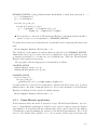
The initial values can be provided in different ways (see the ordinary admb manual). Here,
we only describe the .pin file approach. The .pin file should contain legal values (within the
bounds) for all the parameters, including the random effects. The values must be given in
the same order as the parameters are defined in the .tpl file. The easiest way of generating
a .pin file with the right structure is to first run the program with a -maxfn 0 option (for
this, you do not need a .pin file), then copy the resulting .p01 file into .pin file, and then
edit it to provide the correct numeric values. More information about what initial values for
random effects really mean is given in Section 3.7.
2.2
Why random effects?
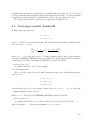
Many people are familiar with the method of least squares for parameter estimation. Far
fewer know about random effects modeling. The use of random effects requires that we
adopt a statistical point of view, where the sum of squares is interpreted as being part of a
likelihood function. When data are correlated, the method of least squares is sub-optimal,
or even biased. But relax—random effects come to rescue!
The classical motivation of random effects is:
• To create parsimonious and interpretable correlation structures.
• To account for additional variation or overdispersion.
We shall see, however, that random effects are useful in a much wider context, for instance,
in non-parametric smoothing.
2.2.1
Statistical prerequisites
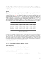
To use random effects in admb, you must be familiar with the notion of a random variable
and, in particular, with the normal distribution. In case you are not, please consult a
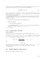
standard textbook in statistics. The notation u ∼ N (µ, σ 2 ) is used throughout this manual,
and means that u has a normal (Gaussian) distribution with expectation µ and variance σ 2 .
The distribution placed on the random effects is called the “prior,” which is a term borrowed
from Bayesian statistics.
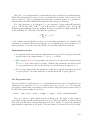
A central concept that originates from generalized linear models is that of a “linear predictor.” Let x1 , . . . , xp denote observed covariates (explanatory variables), and let β1 , . . . , βp
be the corresponding regression parameters to be estimated. Many of the examples in this
manual involve a linear predictor ηi = β1 x1,i + · · · + βp xp,i , which we also will write in vector
form as η = Xβ.
2-4