1
Exercises for the CLUE-S model Peter Verburg, Tom Veldkamp and Jan Peter Lesschen The CLUE-S model Introduction The Conversion of Land Use and its Effects modelling framework (CLUE) (Veldkamp and Fresco, 1996; Verburg et al., 1999) was developed to simulate land use change using empirically quantified relations between land use and its driving factors in combination with dynamic modelling of competition between land use types. The model was developed for the national and continental level and applications for Central America, Ecuador, China and Java, Indonesia are available. For study areas with such a large extent the spatial resolution for analysis was coarse and, as a result, each land use is represented by assigning the relative cover of each land use type to the pixels. Land use data for study areas with a relatively small spatial extent is often based on land use maps or remote sensing images that denote land use types respectively by homogeneous polygons or classified pixels. This results in only one dominant land use type occupying one unit of analysis. Because of the differences in data representation and other features that are typical for regional applications, the CLUE model cannot directly be applied at the regional scale. Therefore the modelling approach has been modified and is now called CLUE-S (the Conversion of Land Use and its Effects at Small regional extent). CLUE-S is specifically developed for the spatially explicit simulation of land use change based on an empirical analysis of location suitability combined with the dynamic simulation of competition and interactions between the spatial and temporal dynamics of land use systems. More information on the development of the CLUE-S model can be found in Verburg et al. (2002) and Verburg and Veldkamp (2003). Model structure The model is sub-divided into two distinct modules, namely a non-spatial demand module and a spatially explicit allocation procedure (Figure 1). The non-spatial module calculates the area change for all land use types at the aggregate level. Within the second part of the model these demands are translated into land use changes at different locations within the study region using a raster-based system. The user-interface of the CLUE-S model only supports the spatial allocation of land use change. For the land use demand module different model specifications are possible ranging from simple trend extrapolations to complex economic models. The choice for a specific model is very much dependent on the nature of the most important land use conversions taking place within the study area and the scenarios that need to be considered. The results from the demand module need to specify, on a yearly basis, the area covered by the different land use types, which is a direct input for the allocation module. 2 Figure 1. Overview of the modelling procedure The allocation is based upon a combination of empirical, spatial analysis and dynamic modelling. Figure 2 gives an overview of the information needed to run the CLUE-S model. This information is subdivided into four categories that together create a set of conditions and possibilities for which the model calculates the best solution in an iterative procedure. The next sections discuss each of the boxes: spatial policies and restrictions, land use type specific conversion settings, land use requirements (demand) and location characteristics. Spatial policies and restrictions Spatial policies and land tenure can influence the pattern of land use change. Spatial policies and restrictions mostly indicate areas where land use changes are restricted through policies or tenure status. For the simulation maps that indicate the areas for which the spatial policy is implemented must be supplied. Some spatial policies restrict all land use change in a certain area, e.g., a log-ban within a forest reserve. Other land use policies restrict a set of specific land use conversions, e.g., residential construction in designated agricultural areas or permanent agriculture in the buffer zone of a nature reserve. The conversions that are restricted by a certain spatial policy can be indicated in a land use conversion matrix: for all possible land use conversions it is indicated if the spatial policy applies. 3 Figure 2. Overview of the information flow in the CLUE-S model Land use type specific conversion settings Land use type specific conversion settings determine the temporal dynamics of the simulations. Two sets of parameters are needed to characterize the individual land use types: conversion elasticities and land use transition sequences. The first parameter set, the conversion elasticities, is related to the reversibility of land use change. Land use types with high capital investment will not easily be converted in other uses as long as there is sufficient demand. Examples are residential locations but also plantations with permanent crops (e.g., fruit trees). Other land use types easily shift location when the location becomes more suitable for other land use types. Arable land often makes place for urban development while expansion of agricultural land occurs at the forest frontier. An extreme example is shifting cultivation: for this land use system the same location is mostly not used for periods exceeding two seasons as a consequence of nutrient depletion of the soil. These differences in behaviour towards conversion can be approximated by conversion costs. However, costs cannot represent all factors that influence the decisions towards conversion such as nutrient depletion, esthetical values etc. Therefore, for each land use type a value needs to be specified that represents the relative elasticity to change, ranging from 0 (easy conversion) to 1 (irreversible change). The user should decide on this factor based on expert knowledge or observed behaviour in the recent past. The second set of land use type characteristics that needs to be specified are the land use type specific conversion settings and their temporal characteristics. These settings are specified in a conversion matrix. This matrix defines: • To what other land use types the present land use type can be converted or not (Figure 3). • In which regions a specific conversion is allowed to occur and in which regions it is not allowed. • How many years (or time steps) the land use type at a location should remain the same before it can change into another land use type. This can be relevant in case of the re-growth of forest. Open forest cannot change directly into closed 4 • forest. However, after a number of years it is possible that an undisturbed open forest will change into closed forest because of re-growth. The maximum number of years that a land use type can remain the same. This setting is particularly suitable for arable cropping within a shifting cultivation system. In these systems the number of years a piece of land can be used is commonly limited due to soil nutrient depletion and weed infestation. It is important to note that only the minimum and maximum number of years before a conversion can or should happen is indicated in the conversion table. The exact number of years depends on the land use pressure and location specific conditions. The simulation of these interactions combined with the constraints set in the conversion matrix will determine the length of the period before a conversion occurs. Figure 4 provides an example of the use of a conversion matrix for a simplified situation with only three land use types. Figure 3. Illustration of the translation of a hypothetical land use change sequence into a land use conversion matrix Figure 4. Example of a land use conversion matrix with the different options implemented in the model 5 Land use requirements (demand) Land use requirements (demand) are calculated at the aggregate level (the level of the case-study as a whole) as part of a specific scenario. The land use requirements constrain the simulation by defining the totally required change in land use. All changes in individual pixels should add up to these requirements. In the approach, land use requirements are calculated independently from the CLUE-S model itself. The calculation of these land use requirements is based on a range of methods, depending on the case study and the scenario. The extrapolation of trends in land use change of the recent past into the near future is a common technique to calculate land use requirements. When necessary, these trends can be corrected for changes in population growth and/or diminishing land resources. For policy analysis it is also possible to base land use requirements on advanced models of macro-economic changes, which can serve to provide scenario conditions that relate policy targets to land use change requirements. Location characteristics Land use conversions are expected to take place at locations with the highest 'preference' for the specific type of land use at that moment in time. Preference represents the outcome of the interaction between the different actors and decision making processes that have resulted in a spatial land use configuration. The preference of a location is empirically estimated from a set of factors that are based on the different, disciplinary, understandings of the determinants of land use change. The preference is calculated following: Rki = akX1i + bkX2i + ..... where R is the preference to devote location i to land use type k, X1,2,... are biophysical or socio-economical characteristics of location i and ak and bk the relative impact of these characteristics on the preference for land use type k. The exact specification of the model should be based on a thorough review of the processes important to the spatial allocation of land use in the studied region. A statistical model can be developed as a binomial logit model of two choices: convert location i into land use type k or not. The preference Rki is assumed to be the underlying response of this choice. However, the preference Rki cannot be observed or measured directly and has therefore to be calculated has a probability. The function that relates these probabilities with the biophysical and socio-economic location characteristics is defined in a logit model following: P Log i 1 − Pi = β 0 + β 1 X 1,i + β 2 X 2,i ...... + β n X n ,i where Pi is the probability of a grid cell for the occurrence of the considered land use type on location i and the X's are the location factors. The coefficients (β) are estimated through logistic regression using the actual land use pattern as dependent variable. This method is similar to econometric analysis of land use change, which is very common in deforestation studies. In econometric studies the assumed behaviour is profit maximization, which limits the location characteristics to (agricultural) economic factors. In the study areas is assumed that locations are devoted to the land use type with the highest 'suitability'. 'Suitability' includes the monetary profit, but can also include cultural and other factors that lead to deviations from (economic) rational behaviour in land allocation. This assumption makes it possible to include a wide variety of location characteristics or their proxies to estimate the logit function that defines the relative probabilities for the different land use types. 6 Most of these location characteristics relate to the location directly, such as soil characteristics and altitude. However, land management decisions for a certain location are not always based on location specific characteristics alone. Conditions at other levels, e.g., the household, community or administrative level can influence the decisions as well. These factors are represented by accessibility measures, indicating the position of the location relative to important regional facilities, such as the market and by the use of spatially lagged variables. A spatially lagged measure of the population density approximates the regionally population pressure for the location instead of only representing the population living at the location itself. Allocation procedure When all input is provided the CLUE-S model calculates, with discrete time steps, the most likely changes in land use given the before described restrictions and suitabilities. The allocation procedure is summarized in Figure 5. The following steps are taken to allocate the changes in land use: 1. The first step includes the determination of all grid cells that are allowed to change. Grid cells that are either part of a protected area or presently under a land use type that is not allowed to change are excluded from further calculation. Also the locations where certain conversions are not allowed due to the specification of the conversion matrix are identified. 2. For each grid cell i the total probability (TPROPi,u) is calculated for each of the land use types u according to: TPROPi ,u = Pi ,u + ELAS u + ITERu where Pi,u is the suitability of location i for land use type u (based on the logit model), ELASu is the conversion elasticity for land use u and ITERu is an iteration variable that is specific to the land use type and indicative for the relative competitive strength of the land use type. ELASu, the land use type specific elasticity to change value, is only added if grid-cell i is already under land use type u in the year considered. 3. A preliminary allocation is made with an equal value of the iteration variable (ITERu) for all land use types by allocating the land use type with the highest total probability for the considered grid cell. Conversions that are not allowed according to the conversion matrix are not allocated. This allocation process will cause a certain number of grid cells to change land use. 4. The total allocated area of each land use is now compared to the land use requirements (demand). For land use types where the allocated area is smaller than the demanded area the value of the iteration variable is increased. For land use types for which too much is allocated the value is decreased. Through this procedure it is possible that the local suitability based on the location factors is overruled by the iteration variable due to the differences in regional demand. The procedure followed balances the bottom-up allocation based on location suitability and the top-down allocation based on regional demand. Steps 2 to 4 are repeated as long as the demands are not correctly allocated. When allocation equals demand the final map is saved and the calculations can continue for the next time step. Some of the allocated changes are irreversible while others are dependent on the changes in earlier time steps. Therefore, the simulations tend to result in complex, non-linear changes in land use pattern, characteristic for complex systems. 7 Figure 5. Flow chart of the allocation module of the CLUE-S model 8 Background of the case study Background of the case study Sibuyan Island For these exercises the case study of Sibuyan Island is used. Sibuyan Island is located in the Romblon Province in the Philippines (Figure 6). The island measures 28 km east to west at its widest point and 24 km north to south, with a land area of approximately 456 km2 surrounded by deep water. Steep mountain slopes covered with forest canopy characterize the island. The land surrounding the high mountains slopes gently to the sea and is mainly used for agricultural, mining and residential activities. The island was selected as a case study because of its very rich biodiversity. About 700 vascular plant species live on Sibuyan Island including 54 endemic to the island and 180 endemic to the Philippine archipelago. Fauna diversity is low, but endemism is high. This makes the island a 'hot spot' for nature conservation and relevant for a detailed study of land use change. For this application a spatial resolution of 250 × 250 meter is used. Five different land use types are distinguished for the simulation (Table 1). The Philippines N Luzon Manila * Sibuyan Island Magdiwang Visayas ~ Espana Pa la wa n Cebu Cajidiocan * San Fernando 2 0 2 4 6 Kilometers Mindanao Figure 6. Location of Sibuyan Island Table 1. Land use types on Sibuyan Island Land use Land use type code Forest 0 Coconut plantations 1 Grassland 2 Rice fields 3 Others 4 (mangrove/beach/villages/etc.) 9 N Four different files with land requirements (demand) scenarios have been created for the period from 1997 to 2011. The land requirements are not very realistic for this short time period, but allow us to clearly analyse the differences between the scenarios. Figure 7 summarizes the land requirements defined in the four scenarios: 1. Slow growth scenario, in this scenario a continuation of the land transformation rates of the past ten years is assumed, meaning deforestation and an increase in the area of coconut plantations, grassland and rice-area. 2. Fast growth scenario, in this scenario a higher rate of land transformation is assumed, leading to rapid conversions of forest to coconut, grassland and rice fields. 3. Food-focus scenario, a high rate of land transformation is foreseen, however, compared to the 'fast growth scenario' relatively more land is dedicated to rice cultivation in order to supply food for the population of the island. 4. Export oriented scenario, the same high land conversion rate applies. However, it is assumed that high copra prices make it profitable to dedicate most land to coconut plantations and less land to food crops. 35000 1997 30000 slow fast 25000 food export 20000 15000 10000 5000 0 forest coconut grassland rice Figure 7. Demands for each land use type 10 others Exercise 1: Learning to know the user-interface This exercise makes you familiar with the user-interface of CLUE-S. The precise definition of the different parameters and input files is discussed in other exercises and in the user manual. 1.0 INSTALLING CLUE-S Extract the file 'setupdemo.zip' this file to a folder on your computer and run setup.exe. This will install CLUE-S on your computer. All files will be installed in a directory you specify during the setup process. It is possible to run CLUE-S from this directory or directly from the 'Start' menu. All files used and created during the simulation should be located in the same directory. 1.1 START CLUE-S CLUE-S can be started in two different ways: 1. Click Start | Programs | CLUE-S tools | CLUE-S 2. Open the directory where CLUE-S is installed with explorer and double-click ‘clues.exe’ The user-interface should appear on the screen (Figure 8). The “Neighborhood Result” and “Neighborhood setting” buttons only appear after checking the “Neighborhood variables” checkbox. These functions are not used in the exercises. A description of the functions can be found in the CLUE-S manual. Figure 8. Interface of the CLUE-S model 11 1.2 MAIN FUNCTIONS The user interface makes it possible to edit the main input files through a built-in text editor and allows the user to choose the scenario conditions. When all parameters are set the simulation can start by clicking the ‘Run CLUE-S’ button. Simulation results will be saved to output files that can be imported by a GIS for display and analysis. Figure 9. Explanation of the CLUE-S interface 1.3 START THE SIMULATION • • Make sure that all input files are correctly defined (correct input files for Sibuyan Island are supplied with the DEMO version) Select an ‘area restriction’ input file The ‘area restriction’ file indicates which cells of a rectangular grid are part of the case-study area and can also contain information on the locations that belong to an area with restrictions to land use conversion, e.g. a natural park. • Select a ‘land requirements’ (demand) input file The ‘land requirements’ file contains for each year that is simulated the required area of the different land use types. These claims can be calculated in other models or can be based on trend extrapolation and demographic projections. Different land requirements are possible for different scenarios. • Click ‘Run CLUE-S’. The simulations will now start and the status bars show the progress (Figure 10). NOTE: The status-bar for the iterative procedure shows the average difference between the allocated area of the different land use types and the required allocation of the different land use types. The simulation of one year is finished if the allocated area deviates less than the specified maximum allowed deviation. Only when one of the land use types exceeds the specified maximum deviation between allocation and requirements for one of the land use types the iterations will continue and a special indicator will appear on the screen. 12 Figure 10. Explanation of the CLUE-S model run 1.4 END OF THE SIMULATION When all simulations are made successfully the model will display the message ‘finished’ and a button that gives access to the LOG-file will appear (Figure 11). The log file contains information on the input files and run-time information on the iterations and may be consulted when errors occur or unexpected results are found. Figure 11. Interface after finishing the simulation 13 1.5 DISPLAY OF SIMULATION RESULTS All results of the simulation are saved in the installation directory. To display the simulation results it is needed to use a GIS package. In this tutorial we will use the ArcView package with the Spatial Analyst Extension. Follow the steps below to display a land use map generated by the CLUE-S model: • Start ArcView and make sure that the Spatial Analyst extension is installed and activated: File | Extensions | Check ‘Spatial Analyst’ | OK • Open a new View by selecting ‘Views’ from the project window and click the ‘New’ button. • Import the file with simulation results that you want to display: File | Import Data Source. Select import file type: ASCII Raster | OK. • Select the file with simulation results. Go to the installation directory of CLUE-S. Note: the installation directory should not contain spaces or special characters, since this might disturb the import of ASCII files in ArcView. Set ‘List Files of Type:’ at ‘All Files (*.*)’. The simulation results are stored in files called: cov_all.* where * indicates the year after the start of the simulation. Select the file you want, e.g. cov_all.10 and click ‘OK’. • Specify a name and directory where you want to store the resulting grid, e.g., YEAR10. • The program will prompt: ‘Cell values as integers?’. Click: ‘Yes’. • The program will prompt: ‘Add grid as theme to the View?’. Click: ‘Yes’. • The result of the simulation can now be seen on the screen and analysed using ArcView (Figure 12). Figure 12. Simulation result displayed in ArcView 14 It is now possible to change the graphical presentation by changing the colours of the map into colour that are easily associated with the different land use type. In the demo-version of the model for Sibuyan Island the suggested colours of Table 2 can be used. Table 2. Land use types with suggested colours Land Land use type use code Forest 0 Coconut plantations 1 Grassland 2 Rice fields 3 Others (Mangrove/Beach/Villages 4 etc.) Suggested colour Dark green Orange Light green Blue Red Î Prepare maps of the results for different years of the simulation with the data supplied with the DEMO version of the CLUE-S model. 15 Exercise 2: Simulate your own scenario 2.1 SCENARIO CONDITIONS The CLUE-S model has a number of parameters that need to be specified before a simulation can be made. The setting of these parameters is dependent on the assumptions made for a particular scenario. In this exercise we will explore 4 different scenario conditions: 1. Land requirements 2. Spatial policies (area restrictions) 3. Conversion elasticity 4. Land use conversion sequences Different scenarios allow the comparison of different possible developments and give insight in the functioning of the model. Such analysis is most easy by visual comparison or through the calculation of the differences between the two scenarios in a GIS. Î Run the model with the baseline scenario: use the original settings of the ‘main parameters’, select ‘region_nopark’ and ‘demand.in1’. Import the results (e.g. for the start and end of the simulation, year 0 and year 14) and run the model again with alternative settings as specified in the following sections (2.2 to 2.5). Compare the results in ArcView. Prepare a short presentation of the observed differences between the scenarios. ArcView maps can be exported to other graphical formats by: File | Export. Select the Windows Bitmap (*.bmp) format for the best results. Figure 13. Simulation results for two different scenarios 16 2.2 LAND REQUIREMENTS The land requirements are input to the model. For each year of the simulation these requirements determine the total area of each land use type that needs to be allocated by the model. The iterative procedure will ensure that the difference between allocated land cover and the land requirements is minimized. Land requirements are calculated independently from the CLUE-S model itself, which calculates the spatial allocation of land use change only. The calculation of the land use requirements can be based on a range of methods, depending on the case study and the scenario. The extrapolation of trends of land use change of the recent past into the near future is a common technique to calculate the land use requirements. When necessary, these trends can be corrected for changes in population growth and/or diminishing land resources. For policy analysis it is also possible to base the land use requirements on advanced models of macro-economic changes, which can serve to provide scenario conditions that relate policy targets to land use change requirements. Simulating scenarios with different land requirements Four different files with land requirements are provided with the model for the period from 1997 to 2011. The land requirements in these scenarios are not very realistic for this short time period but allow us to clearly analyse the differences between the scenarios. The scenarios are based on the following assumptions: demand.in1: demand.in2: demand.in3: demand.in4: Slow growth scenario, in this scenario a continuation of the land transformation rates of the past ten years is assumed, meaning deforestation and an increase in the area of coconut plantations, grassland and rice fields. Fast growth scenario, in this scenario a higher rate of land transformation is assumed, leading to rapid conversions of forest to coconut, grassland and rice fields. Food-focus scenario, a high rate of land transformation is foreseen, however, compared to the 'fast growth scenario' relatively more land is dedicated to rice cultivation in order to supply food for the population of the island. Export oriented scenario, the same high land conversion rate applies. However, it is assumed that high copra prices make it profitable to dedicate most land to coconut plantations and less land to food crops. Î Select one of the land requirement scenarios and run the model keeping all other settings equal to the first run of the model. Analyse the results wit ArcView through displaying the land use pattern at the start of the simulation and at the end of the simulation. Repeat this for another scenario of land requirements and compare the results. NOTE: Each simulation, the model will overwrite the results of a previous simulation. If you want to save the results, rename the output files or move the output files to another directory. Î Define your own scenario by generating a new land requirements input file for CLUE-S. Follow the steps below: • Open Microsoft Excel to facilitate the calculations. • Specify for each year (1997-2011) the land requirements of the different land use types in a table following the specifications below: - Each row indicates a year; each column a land use type following the order of the land use coding. - Make sure to include also the land requirements for 1997 (year 0). These should be similar to the land use map of 1997 (29518.75, 7237.5, 5243.75, 1400, 1762.5 ha for respectively forest, coconut, grassland, rice and others). 17 - The total land area required should equal the size of the island (45162.5 ha), i.e., the sum of the values on each row should equal 45162.5 for each year. We suggest not to change the land use requirements for the ‘others’ land use class and to create logical scenarios without sharp increases or decreases. This should prevent problems or very long run times during the simulation. • When all values have been defined, select the values (without land use type names and year numbers) and paste the contents into a text editor (e.g. Notepad). Insert a line at the top of the file with the number of lines (years) for which the land requirements are specified (15 in our example). • Save this file in the installation directory as ‘demand.in*’ where * can be defined by the users, e.g. demand.in5. Restart the CLUE-S model; it is now possible to select the new land requirement file and simulate the land use changes. Analyse the results. • • 18 2.3 SPATIAL POLICIES (AREA RESTRICTIONS) This option indicates areas where land use changes are restricted through spatial (land use) policies or tenure status. Maps that indicate the areas for which the spatial policy is implemented must be supplied. Some spatial policies restrict all land use change in a certain area, e.g., when in a forest reserve all logging is banned. Other land use policies restrict a set of specific land use conversions, e.g., residential construction in designated agricultural areas. In this exercise we will only address policies that restrict all land use changes in designated areas. With the DEMO version of the model we supply three area restriction files that can be selected through the user-interface. Each file contains a map designating the areas where land use change is restricted. The maps are shown in Figure 14 but can also be imported in ArcView as ASCII Raster file similar to the procedure used to import the results of the simulations. The files are located in the installation directory. Area restriction files: region_nopark.fil: no spatial policies included. region_park1.fil: one large nature park following the boundaries of the Department of Environment and Natural Resources of the Philippines region_park2.fil: instead of one large nature park protection is proposed for small areas which are assumed to face large land use change pressure. Figure 14. Maps of restricted areas (in black) Î Run the CLUE-S model with the different area restriction files keeping all other settings equal to the first run of the model. Compare the results with the initial situation (1997, year 0) and compare the impact of the different area restrictions. • Is strict protection of the nature reserve needed for the developments until 2011 as simulated by the model? • Do the protected areas in ‘park 2’ protect areas that would otherwise be deforested? What is the consequence of strictly protecting these areas? NOTE: Each simulation, the model will overwrite the results of a previous simulation. If you want to save the results, rename the output files or move the output files to another directory. 19 2.4 CONVERSION ELASTICITY The conversion elasticity is one of the land use type specific settings that determine the temporal dynamics of the simulation. The conversion elasticity is related to the reversibility of land use changes. Land use types with high capital investment or irreversible impact on the environment will not easily be converted in other uses as long as there are land requirements for those land use types. Such land use types are therefore more ‘static’ than other land use types. Examples of relatively static land use types are residential areas, but also plantations with permanent crops (e.g., fruit trees). Other land use types are more easily converted when the location becomes more suitable for other land use types. Arable land often makes place for urban development while expansion of agricultural land can occur at the same time at the forest frontier. An extreme example is shifting cultivation: for this land use system the same location is mostly not used for periods exceeding two seasons as a consequence of nutrient depletion of the soil. These differences in behaviour towards conversion of the different land use types can be approximated by the conversion costs. However, costs cannot represent all factors that influence the decisions towards conversion such as nutrient depletion, esthetical value etc. Therefore, in the model we have assigned each land use type a dimensionless factor that represents the relative elasticity to conversion, ranging from 0 (easy conversion) to 1 (irreversible change). The user should specify this factor based on expert knowledge or observed behaviour in the recent past. An extended explanation of the possible values of the conversion elasticity and how behaviour changes when the land requirements increase or decrease in time is given below. 0: >0...<1: 1: Means that all changes for that land use type are allowed, independent from the current land use of a location. This means that a certain land use type can be removed at one place and allocated at another place at the same time, e.g. shifting cultivation. Means that changes are allowed, however, the higher the value, the higher the preference that will be given to locations that are already under this land use type. This setting is relevant for land use types with high conversion costs. Means that grid cells with one land use type can never be added and removed at the same time. This is relevant for land use types that are difficult to convert, e.g., urban settlements and primary forests. A value of one stabilizes the system and prevents that in case of deforestation other areas are reforested at the same time. The conversion elasticity is specified in the ‘Main Parameters’ input file that can be edited through the user interface (click the ‘Main Parameters’ button) or with a text editor in the file ‘main.1’ in the installation directory. The conversion elasticity of all land use types is specified on line 11 of this file (an explanation of all other parameters in this file can be found in the user manual). The first conversion elasticity corresponds with land use type 0, the second with land use type 1, etc. Table 3. Current settings of the conversion elasticities Land use type Conversion elasticity 1 Forest (0) 0.8 Coconut plantations (1) 0.2 Grassland (2) 0.2 Rice fields (3) 1 Others (4) Î Run the baseline scenario for Sibuyan island with the CLUE-S model with the current settings and with alternative settings for the conversion elasticity. Change the conversion elasticity by: 20 • • Click on the ‘Main Parameters’ button. The main parameters can now be edited. Line 11 contains the conversion elasticity settings of the different land use types in the same order as the land use type coding. Change these values to new values. • • Click on ‘Save’. Run the model after selecting the ‘Area restrictions file’ and the ‘Land requirements’ file (similar to the first run of the model). Display the results with ArcView. Compare the differences in spatial pattern of land use change as result of the changes in conversion elasticity. • • NOTE: Each simulation, the model will overwrite the results of a previous simulation. If you want to save the results, rename the output files or move the output files to another directory. 21 2.5 LAND USE CONVERSION SEQUENCES Not all land use changes are possible and some land use changes are very unlikely (e.g., arable land cannot be converted into primary rain forest). Many land use conversions follow a certain sequence or cycle, e.g. fallow land and forest regrowth often follow shifting cultivation. Figure 15 indicates a number of possible land use trajectories identified on Sibuyan island. ion defores tatio n deforestation/logging grass regrowth /log gi n g r e gr secondary forest ow nt primary forest primary forest th vat ser con shifting cultivation ag ri cu lt u ral ex p ans aband on m e l ra u lt u o n c i r g i a ns expa permanent agriculture io n Figure 15. Possible land use trajectories on Sibuyan island. The conversions that are possible and impossible are specified in a land use conversion matrix. For each land use type it is indicated in what other land use types it can be converted during the next time step. Figure 16 provides a simplified example of a land use transition sequence. Forest can be converted in either agricultural land or grassland, while it is impossible to obtain new (primary) forest through the conversion of agricultural land or grassland directly. The figure also illustrates the translation of these conversion sequences into a land use conversion matrix, which can be used by the model. Depending on the definition of this conversion matrix and the time-steps chosen, complex land use sequences are possible. (b) logging present land use forest (a) agricultural expansion agriculture (c) abandonment ( d ) re cla m a ti o grassland n Grassland future land use Agriculture Land use conversion matrix Forest Land use change sequence Forest + +(a) +(b) Agriculture - + Grassland - +(e) + +(d) + conversion possible - conversion not possible Figure 16. Land use transition sequence The land use conversion matrix can be edited by clicking the ‘Change matrix’ button. It is also possible to use a text editor (e.g. Notepad) to edit the file ‘allow.txt’ in the installation directory. The rows of this matrix indicate the land use types during time step t and the columns indicate the land use types in time step t+1. If the value of a cell is 1 the conversion is allowed while a 0 indicates that the conversion is not possible. The rows and columns follow the number code of the land use types. 22 Example: in the matrix below all conversion are possible except the conversion from coconut plantation into rice fields. 1 1 1 1 1 1 1 1 1 1 1 1 1 1 1 1 0 1 1 1 1 1 1 1 1 Code 0 1 2 3 4 Land use type Forest Coconut plantations Grassland Rice fields Others Î Run the baseline scenario for Sibuyan island with a different setting of the conversion matrix (keeping all other settings equal) and analyse the differences in outcome with ArcView. We suggest to compare a model run that allows all changes with a model run in which the conversion of grassland into agricultural land (coconut plantation and rice fields) is no longer possible due to soil degradation. Compare the results. Note: Some land use conversion settings will have no effect because they are overruled by the conversion elasticity and land requirement settings. In the baseline scenario we have assumed that the ‘others’ land use type is not changing and forest cannot ‘re-grow’ from other land use types as long as its total land area is decreasing. Changing the conversion settings for these land use types in the conversion matrix will have no effect on the simulation results. Each simulation, the model will overwrite the results of a previous simulation. If you want to save the results, rename the output files or move the output files to another directory. 23 Exercise 3: Defining spatial policies 3.1 INTRODUCTION For some scenarios it is interesting to define areas where land use changes are restricted because of spatial policies, e.g. the conservation of nature. In Section 2.3 we have seen that spatial policies should be defined in an ‘area restriction’ file. This file contains a map of the study area indicating the extent of the case-study area and the zones of the case-study area where spatial restrictions apply. The ‘area restriction’ file is located in the installation directory and called ‘region*.fil’ where * can be defined by the user to indicate the conditions specified in the file. With the DEMO version of CLUE-S three different area restriction files are supplied, one without any spatial policy and two file indicating different extents of a nature reserve. Î Import these ‘area restriction’ files in ArcView using File | Import Data Source | ASCII Raster. In this exercise we will create a new ‘area restriction’ file to simulate a scenario of the effects of a strict protection of all remaining lowland forest on Sibuyan island. Therefore we assume that during the simulations it is not possible to convert any of the remaining forest areas below an altitude of 100 meter. PREPARATION OF THE AREA RESTRICTION FILE To make the area restriction file we need to identify: • The extent of the case study • The locations below 100 meter altitude • The locations with forest at the start of the simulations Therefore it is needed to import the land use map of year 0 (the start of simulations) in ArcView. This land use map shows the extent of the study area grid-cells that are designated to a land use type) and the locations with forest at start of the simulations. This land use map can be found (in ASCII format) in installation directory and is called <cov_all.0>. the (all the the To identify the locations below 100 meter an altitude map is needed. Since altitude is one of the location factors used in the simulations for Sibuyan island this map is already present in the installation directory. For this case study altitude is location factor number 7 in file ‘sc1gr7.fil’. Î Import the ASCII files of land use at the start of the simulation and altitude in ArcView. 24 Select all locations with forest located below an altitude of 100 meter at the start of the simulation by a ‘map query’ (Analysis | Map Query) (Figure 17). This will result in a new theme indicating all selected locations. Figure 17. Map query with ArcView In the ‘area restriction’ file the following coding should be used: 0: all grid cells that belong to the study area outside the ‘restricted area’ -9998: all grid cells for which land use conversions are not allowed during the simulations (the ‘restricted area’) ‘No Data’ or -9999: all other grid cells (outside the simulation area) Î Prepare an ‘area restriction’ file. You can follow the steps below or use your own procedure: 1. Classify the land use map of year 0 to identify all cells inside the case study area (reclassify all land use types to 0; Analysis | Reclassify). 2. Overlay the result with the forest areas below 100 meter. This can be done by the Map Calculator (Analysis | Map Calculator). 3. The result only needs to be reclassified to the coding system of the area restriction file, as listed above (Analysis | Reclassify). 4. Save this theme as a grid (Theme | Save Data Set). 5. Export this theme as an ASCII file (File | Export Data Source) into the installation directory with a name following ‘region*.fil’ (where * can be defined by the user). 25 SIMULATE LAND USE CHANGE Î If you restart the CLUE-S model the new area restriction file should appear in the list of area restriction files and can be selected for the simulations. Run the model with the new area restriction file and compare the result with a simulation without protection of forest resources. Î Prepare your own area restriction file based on a hypothetical spatial policy. You can also prepare area restriction files by delineating areas in ArcView that need to be converted to grid cells. Note: If the area restrictions violate the land requirements specified in the ‘land requirements’ file the model will not succeed in allocating land use changes and stop the simulation. This can occur when all forest is assumed to be protected while at the same time a decrease in land requirements for forest is specified. 26 Exercise 4: How to do the statistical analysis? INTRODUCTION The CLUE-S model uses a statistical analysis to define the suitability of locations for different land use types. The suitability of a location is a function of a number of casestudy specific location factors, such as soil quality, accessibility, socio economic conditions etc. In this exercise a statistical analysis will be made to relate these location factors to the suitability of the different land use types by a logit model. FILE CONVERSION For the statistical analysis standard statistical packages need to be used. Since most of these packages do not support the use of GIS data directly a number of conversions are needed to translate the data format of GIS packages into the data format supported by the statistical packages. With the CLUE-S model a small application is supplied (convert.exe) that helps to make this conversion. Basically, it is able to translate ArcView/ArcGIS ASCII grids into a tabular format that can be imported by most statistical programs. In this exercise we will import the land use map and the driving factors into SPSS for statistical analysis. The following ArcView/ArcGIS ASCII grid files are available with the demo version: Table 4. Available land use type and driving factor files Filename Description Forest Cov1_0.0 Coconut plantations Cov1_1.0 Grassland Cov1_2.0 Rice fields Cov1_3.0 Others (mangrove/Beach/Villages etc.) Cov1_4.0 Distance to sea Sc1gr0.fil Mean population density (village territory) Sc1gr1.fil Geology: diorite rock Sc1gr2.fil Geology: ultramafic rock Sc1gr3.fil Geology: sediments Sc1gr4.fil Erosion: no erosion Sc1gr5.fil Erosion: moderate erosion Sc1gr6.fil Elevation Sc1gr7.fil Slope Sc1gr8.fil Aspect Sc1gr9.fil Distance to road Sc1gr10.fil Distance to city Sc1gr11.fil Distance to stream Sc1gr12.fil These files can be imported in ArcView through File | Import Data Source | ASCII Raster. Î Import some of the maps of the driving factors to see their spatial distribution. Î Prepare for each of the land use types (except for the ‘others’ land use type) a hypothesis of the potential factors (from the list above) that might influence the suitability of a location for that land use type. 27 Î Convert all files needed to estimate the statistical relation between the location of land use and the hypothesized location factors following the steps below: • Open the File Convert program by double clicking ‘convert.exe’ in the installation directory. The user-interface will appear: • Click on the ‘edit file list’ button to open a text file (names.txt) that contains the names of all files that need to be converted. Edit this text file to include all files needed. The first line of the file should specify respectively the maximum number of files that need to be converted in one run and the maximum number of observations in these files. The following lines should specify the full names of the files. Click on the ‘save file list’ button to save the changes and close the text editor. • To delete all NODATA values from the grid files check the ‘Exclude NODATA values’ option. Note: Only use this option if you are sure that all files have exactly the same number of NODATA values at the same geographical locations. • To produce a file that lists all data values of the different files in a tabular format with the files in columns and the observations in rows check the ‘Make stat-file’ option. This file has the necessary format for data import in most statistical packages. Click the ‘Start conversion’ button to run the conversion. When the conversions are finished you can exit the File Convert program. • • The results are saved in two formats: 1. For every file a new file is created named ‘c-*’ where * stands for the original filename. This file contains all grid data in one column with or without NODATA values depending on the selected option. 2. A file called ‘stat.txt’ that contains data in tabular format. Each column contains the values of a file (first column: first file etc.); each row contains the values for a single grid cell for all files (Figure 18). 28 Figure 18. Format of the ‘stat.txt’ file 4.3 PERFORMING THE STATISTICAL ANALYSIS In this exercise we use SPSS to do the statistical analysis. Î Import the ‘stat.txt’ data file into SPSS by starting the SPSS software and selecting: ‘File | Read Text Data’ and select the just produced file ‘stat.txt’ and go through the import wizard. This will import all data. The names of the columns are not imported and should be specified by the user. The order of the columns equals the order of the files specified in the File Convert program. In SPSS it is possible to edit the names in the ‘Variable View’ tab. This will facilitate the analysis. Î Perform a logistic regression analysis to test the hypotheses you have specified for the different land use types • • • Click: Analyze | Regression | Binary Logistic. Select a land use type as dependent variable and the location factors you have selected as independent variable. Categorical variables should be identified with the ‘Categorical’ button. Select a method for regression: ‘Enter’ if you want to include all selected variables or one of the other methods for stepwise regression. Select for this exercise the ‘Forward: Conditional’ method. 29 • • • • Click the ‘Save’ button and check the probabilities option to save the predicted probabilities. Click the ‘Options’ button to set the conditions for stepwise regression. In the ‘probability for stepwise’ section you can indicate the significance values for Entry and Removal during the stepwise procedure. For large data sets these values can be set at respectively 0.01 and 0.02. Run the regression by clicking ‘OK’. Output will be generated in a special window. Use the help function if you have problems interpreting the output. Figure 19. Output section of the logistic regression with SPSS The ‘Variable in the equation’ table in the ‘Block 1’ output section contains the resulting logit model (Figure 19). The β values for the driving factors are the values in the column B for the last step, in the example of Figure 14 the β value for population density (POPDENS) is 0.001. By default only 3 decimals are shown, this number can be increased in the Cell properties window. Select the specific cells and go to ‘Format | Cell Properties’. 30 4.4 EVALUATING THE GOODNESS OF FIT WITH THE ROC METHOD The ROC characteristic is a measure for the goodness of fit of a logistic regression model similar to the R2 statistic in Ordinary Least Square regression (Pontius and Schneider, 2001). A completely random model gives a ROC value of 0.5; a perfect fit results in a ROC value of 1.0. Î Calculate the ROC value for your regression model. • Click: Graphs | ROC Curve. Select the observed land use as ‘State variable’ with value 1 for occurrence of this land use type and the ‘Predicted probability’ as ‘Test variable’. Click ‘OK’. • The results will show a ROC curve and the ‘area under the curve’ that is the test result (Figure 20). Figure 20. ROC curve of a logistic regression with SPSS 31 4.5 USING THE REGRESSION RESULTS AS INPUT TO THE CLUE-S MODEL The regression results are used by the CLUE-S model to determine the suitability of the locations for the different land use types. For each land use type considered a separate regression model is used. The result of the analysis in SPSS should therefore be translated to input for the CLUE-S model. The input file for the regression equations is called ‘alloc1.reg’ and is located in the installation directory and can be edited through the user interface of CLUE-S. Figure 21. Editor for the regression results This file is structures as follows (Figure 22): Line 1: Number code for land use type (e.g. forest). Line 2: Constant of regression equation for land use type (ß0). Line 3: Number of explanatory factors (sc1gr#.fil files) in the regression equation for that land use type. Line 4 and On each line the beta coefficients (ß1, ß2, etc.) for the explanatory factor further: and the number code of the explanatory factor. Number code of land use type Constant Number of explanatory factors Number code of explanatory factor (e.g. population) Beta value for explanatory factor Figure 22. Structure of the regression results file (alloc1.reg) 32 Î Use the output of your regression analysis to change the input file for CLUE-S. • Use the coding of the land use types used in this DEMO version: Code 0 1 2 3 4 • Use the coding system of the location factors, similar to the coding used in the filenames ‘sc1gr*.fil’ where * is the code: Code 0 1 2 3 4 5 6 7 8 9 10 11 12 • Land use type Forest Coconut plantations Grassland Rice fields Others Location factor Distance to sea Mean population density (village territory) Geology: diorite rock Geology: ultramafic rock Geology: sediments Erosion: no erosion Erosion: moderate erosion Elevation Slope Aspect Distance to road Distance to city Distance to stream Save the file and run the model with the new settings Î Compare the results of simulations with different location factors included in the regression analysis. Probability maps solely based on the regression equations can be generated with the ‘Calculate probability maps’ button in CLUE-S and are stored in ‘prob1_*.1’ where * indicates the land use code. These maps can be imported as floating point grids in ArcView ‘File | Import Data Source | ASCII Raster’. Note: do not import as integers. Do different regressions result in different probability maps? Do different probability maps result in different simulation results of the land use change model? 33 References Pontius, R.G. and Schneider, L.C. 2001. Land use change model validation by an ROC method for the Ipswich watershed, Massachusetss, USA. Agriculture, Ecosystems andEnvironment, 85: 239-248. Veldkamp, A. and Fresco, L.O. 1996. CLUE-CR: an integrated multi-scale model to simulate land use change scenarios in Costa Rica. Ecological modelling, 91: 231248. Verburg, P.H., Veldkamp, A., de Koning, G.H.J., Kok, K. and Bouma, J. 1999. A spatial explicit allocation procedure for modelling the pattern of land use change based upon actual land use. Ecological modelling, 116: 45-61. Verburg, P.H., Soepboer, W., Veldkamp, A., Limpiada, R. and Espaldon, V. 2002. Modeling the spatial dynamics of regional land use: the CLUE-S model. Environmental Management, 30(3): 391-405. Verburg, P.H. and Veldkamp, A. 2003. Projecting land use transitions at forest fringes in the Philippines at two spatial scales. Landscape Ecology, in press. 34