Download ASPIC 7 User`s Manual

User’s Guide for ASPIC Suite, version 7:
A Stock–Production Model Incorporating Covariates
and auxiliary programs
c c c
Michael H. Prager — Prager Consulting
Portland, Oregon, USA
www.mhprager.com
c c c
Last revised May 6, 2015
Preface
plications and questions.
This guide describes Version 7 of the ASPIC Suite,
a set of computer programs to fit non-equilibrium
stock-production models to fisheries data. The
main program is ASPIC, which does the estimation.
Three utility programs are provided. The role of
ASPICP is to make projections; of AGRAPH, to make
simple graphs from ASPIC and ASPICP output files;
of ASPIC5to7 to convert input files from ASPIC 5 to
ASPIC 7 format.
This user’s guide is a major revision of NMFS Beaufort Lab Document BL–2004–01 (2004), itself a revision of NMFS Miami Lab Document MIA–92/93–55
(1992).
The main changes in ASPIC 7 are additional estimation methods (maximum-likelihood and maximum
a posteriori); revised input-file format to accommodate the new methods; and elimination of some
rarely used options.
A general technical description of the theory behind
ASPIC was given in Prager (1994). The bibliography
(p. 32) has additional references, and this guide now
includes a technical section (§8).
ASPIC has been used in numerous stock assessments and simulation studies. Distribution is made
to fishery scientists without charge, to further fisheries research and education. As with any software,
errors may be present. The author attempts to fix
suspected errors promptly.
The ASPIC Suite carries no warranty of any kind.
Use is entirely at your own risk.
Development of ASPIC has been supported by the
U.S. National Marine Fisheries Service (NMFS) and
by the author’s private efforts, with additional support from the International Commission for the
Conservation of Atlantic Tunas (ICCAT).
This software is distributed to interested scientists
free of charge. No individual or group is authorized to charge for it or distribute it as part of
any commercial product. The author requests that
this manual and Prager (1994) be cited in any report or published article that uses ASPIC.
Many colleagues have given valuable technical suggestions or assistance through the years. I thank
S. Cadrin, R. Deriso, K. Hiramatsu, J. Hoenig, R.
Methot, C. Porch, J. Powers, A. Punt, V. Restrepo,
G. Scott, K. Shertzer, J. Thorson, P. Tomlinson, D.
Vaughan, E. Williams, and the many fishery scientists who have sent data sets to illustrate their ap2
Typographical conventions
In this guide, user commands, file names, and items
in input files are displayed in a monospaced font.
Some important sections are marked by a symbol
in the margin, as here; attention to such material
is especially important to obtaining good results
from ASPIC. Material new in this version of the
program is marked by a different marginal symbol,
as here.
Michael H. Prager, Ph.D.
Prager Consulting
Portland, Oregon, USA
May, 2014
4
V
Contents
Preface
Typographical conventions . . . . . . . . .
2
2
Contents
3
List of Tables
4
List of Figures
4
1 Introduction
5
2 New features
5
3 Compatibility and installation
3.1 Compatibility . . . . . . . . . . . . . . .
3.2 Installation . . . . . . . . . . . . . . . .
3.2.1 NMFS Toolbox version . . . . .
6
6
6
6
4 Overview of ASPIC
4.1 Modeling flow . . . . . . . . . . . . . .
4.2 User Interface . . . . . . . . . . . . . .
4.3 Data requirements . . . . . . . . . . .
4.4 Program limits . . . . . . . . . . . . .
4.5 Program modes . . . . . . . . . . . . .
4.6 Several data series . . . . . . . . . . .
4.7 Choices for fitting . . . . . . . . . . .
4.7.1 Estimation methods . . . . . .
4.7.2 Statistical conditioning . . . .
4.7.3 Penalty for B1 > K . . . . . . .
4.7.4 Residuals and bootstrapping
4.8 Input and output files . . . . . . . . .
4.8.1 Input file . . . . . . . . . . . . .
4.8.2 Output files . . . . . . . . . . .
4.9 Running ASPIC . . . . . . . . . . . . .
.
.
.
.
.
.
.
.
.
.
.
.
.
.
.
7
7
7
7
7
7
9
9
9
9
9
9
10
10
10
11
5 ASPIC 7 input file specification
5.1 Data representations . . . . . . . . . .
5.2 Line-by-line details . . . . . . . . . . . .
* Prior specification . . . . . . . . . .
12
12
13
16
6 Auxiliary Programs
6.1 ASPIC5to7 . . . . . . . . . . . . .
6.2 AGRAPH . . . . . . . . . . . . . .
6.3 ASPICP . . . . . . . . . . . . . . .
6.3.1 ASPICP interface and use
6.3.2 ASPICP control file . . . .
6.3.3 Sample control file . . .
.
.
.
.
.
.
19
19
19
20
20
20
22
7 Tips on using the ASPIC Suite
7.1 Estimation controls . . . . . . . . . . .
22
22
.
.
.
.
.
.
.
.
.
.
.
.
.
.
.
.
.
.
7.1.1 Guesses of q . . . . . . . . . . .
7.1.2 Priors and bounds . . . . . . . .
7.1.3 Starting guesses in bootstraps
7.2 Data issues . . . . . . . . . . . . . . . .
7.2.1 Missing values and zeros . . .
7.2.2 Using several data series . . . .
7.2.3 Allocating yield . . . . . . . . .
7.3 Estimation difficulties . . . . . . . . . .
7.3.1 Monte Carlo search . . . . . . .
7.3.2 Issues with priors . . . . . . . .
7.3.3 Sensitivity to seeds or guesses
7.3.4 Estimation failure . . . . . . . .
7.3.5 Reporting problems . . . . . . .
7.4 Interpretation of ASPIC Results . . . .
7.4.1 Precision of estimates . . . . .
7.4.2 Catchability over time . . . . .
7.4.3 Projections . . . . . . . . . . . .
8 Technical appendix
8.1 Estimation methods—overview . .
8.2 Least-squares estimation . . . . . .
8.2.1 Data-series terms . . . . . .
8.2.2 Penalty for B1 > K . . . . . .
8.2.3 Total SSE . . . . . . . . . . . .
8.3 Least absolute values estimation .
8.3.1 Data-series terms . . . . . .
8.3.2 Penalty for B1 > K . . . . . .
8.3.3 Total LAV . . . . . . . . . . .
8.4 Maximum-likelihood estimation .
8.4.1 Data-series terms . . . . . .
8.4.2 Observation standard error
8.4.3 Penalty for B1 > K . . . . . .
8.4.4 Total likelihood . . . . . . .
8.5 Maximum a posteriori estimation
8.6 Bootstrapping . . . . . . . . . . . . .
8.6.1 Overview . . . . . . . . . . . .
8.6.2 Initial fit . . . . . . . . . . . .
8.6.3 Residual inflation factor . .
8.6.4 Resampling algorithm . . .
8.7 Projections in ASPICP . . . . . . . .
8.7.1 Process variability in MSY .
.
.
.
.
.
.
.
.
.
.
.
.
.
.
.
.
.
.
.
.
.
.
.
.
.
.
.
.
.
.
.
.
.
.
.
.
.
.
.
.
.
.
.
.
22
22
22
23
23
23
23
25
25
25
25
25
26
26
26
27
27
27
28
28
28
28
28
29
29
29
29
29
29
29
29
30
30
30
30
30
30
30
31
31
9 Source code availability
31
References
32
3
List of Tables
1
2
–
–
–
–
3
Data-series types and codes . .
Files used by the ASPIC suite .
Model shape codes . . . . . . .
Conditioning codes . . . . . . .
Objective function codes . . . .
Management codes for ASPICP
Missing values and zeroes . . .
.
.
.
.
.
.
.
.
.
.
.
.
.
.
.
.
.
.
.
.
.
.
.
.
.
.
.
.
10
11
13
14
14
22
24
Modeling flow with ASPIC Suite. . . . .
8
List of Figures
1
4
1
Introduction
This guide describes Version 7 of ASPIC, a computer
program to fit non-equilibrium surplus-production
models to fisheries data. Three utility programs
(ASPIC5to7, ASPICP, AGRAPH) are also described,
whose roles are conversion of input files from ASPIC
5 format, making projections, and making basic
graphs of results. Together, the programs are called
the ASPIC Suite.
The surplus-production model has a long history in
fishery science and has proven useful repeatedly in
assessment of fish stocks (Shertzer et al. 2008). The
appeal of production models is in large part their
conceptual and computational simplicity. Despite
that simplicity, production models incorporate an
implicit recruitment function, and thus can be used
for studies of sustainability. Production models
have also been found especially useful in stock
assessments when the age-structure of the catch
cannot be estimated.
To simplify calculations, early treatments of
surplus-production models assumed that the yield
taken each year could be considered the equilibrium yield (e. g., Fox 1975). However that “equilibrium assumption” tends to overestimate MSY
when assessing a declining stock, and it has been
found problematic in several studies (Mohn 1980;
Williams and Prager 2002). The simplification is no
longer needed, and ASPIC does not use it.
ASPIC 7 fits the logistic production model (Schaefer
1954, 1957; Pella 1967), in which the production
curve1 is symmetrical around BMSY ; the generalized
model of Pella and Tomlinson (1969) as reparameterized by Fletcher (1978); and the Fox exponential
yield model (Fox 1970) as an important special case
of the generalized model.
ASPIC incorporates several notable features:
• Analysis of up to 12 data series, which may
represent different gears or different periods of time. Data accepted include annual
catches, indices of relative abundance, and
estimates of absolute biomass. (See §4.6.)
• Bootstrapping to provide nonparametric confidence intervals on estimated quantities.
• Fitting statistically conditioned on yield, fishing effort, or relative abundance.
• Four objective functions: least squares
(equivalent to concentrated maximum likelihood), least absolute values, maximum likelihood, and maximum a posteriori (ML with
priors).
The theory behind ASPIC and several examples were
first presented in working documents of the International Commission for the Conservation of Atlantic Tunas (ICCAT) by Prager (1992a,b). Those
references were superseded by the more complete
treatment of Prager (1994). The model and its extensions are also described in Quinn and Deriso
(1999) and Haddon (2001). The basic theory of production models is of course also described in many
other texts, including Hilborn and Walters (1992),
and is the subject of at least one FAO publication
(Punt and Hilborn 1996).
The ASPIC computer program as described here has
been used by several assessment groups and in
many studies, including Prager et al. (1996), Prager
and Goodyear (2001), Prager (2002), Shertzer and
Prager (2002), and Williams and Prager (2002). In
the course of those studies, the program has been
exercised on over 100,000 sets of simulated data.
The resulting experience has been used to improve
the program’s reliability.
Version numbers 4 and 6 were reserved for development use. Released versions of ASPIC have included
versions 1, 2, 3, 5, and 7.
Versions of ASPIC before 5.0 are no longer maintained by the author. Version 3 is still available at
the author’s Web site, to allow duplicating historic
analyses, but will be removed some time in 2014.
Version 5 will be maintained along with version
7 for several years, then discontinued. The author
urges analysts to use the most recent version for
new work.
Updates to ASPIC will be made available at the author’s Web site, http://www.mhprager.com for as
long as the author continues to maintain ASPIC.
2
1. The production curve is the plot of theoretical stock production as a function of stock biomass or numbers.
4
New features
This section gives an overview of the most sig5
4
nificant changes introduced between ASPIC 5 and
ASPIC 7.
Estimation methods. Maximum-likelihood and
maximum a posteriori estimation have been added.
Iteratively weighted least-squares has been removed.
Leading parameters. The user now provides starting guesses and bounds (optionally, priors) on MSY
and FMSY instead of MSY and K.
Input file format. The input file format has been
revised and (hopefully) made more logical. A conversion program is supplied for version 5 input
files.
Bounds on q. The user now supplies bounds on
catchability coefficients. In earlier versions of ASPIC,
bounds on q were computed heuristically by the
program.
Data extents. Time series in the input file may now
be up to 150 years long, increased from 100 years.
The maximum number of bootstraps has been increased from 1000 to 3000.
3
Compatibility and installation
3.1
Compatibility
The ASPIC suite is compatible with personal computers running 32-bit or 64- bit versions of Microsoft Windows.2 The author has tested it on Windows 7.0.
ASPIC is written in standard Fortran 95 and is
portable to other operating systems. Please consult the author if you would like to use ASPIC under
operating systems other than Windows. In particular, a Linux version may be available.
are different. The only program with the same
executable-file name is AGRAPH, but AGRAPH is
identical in current copies of both versions.
If you keep both versions on the same computer,
it is recommended to rename the shortcuts of the
older version to include a version number. If you
prefer, you can uninstall and reinstall the ASPIC 5
suite, and this will be done for you.
* The version 7 installer does the following:
• Installs executable files for ASPIC, ASPICP,
ASPIC5to7 and AGRAPH (and support files)
to a location specified by the user. The default location is the ASPIC7 subdirectory
created in the Windows Program Files or
Program Files (x86) tree.
• Installs this User’s Guide and the ASPIC
Quick Start Guide to the doc subdirectory
of the program-installation location.
• Installs sample input and output files
to an ASPIC7Work subdirectory of the
My Documents directory belonging to the
Windows All Users or Public profile.
• Adds the program location to the user’s
PATH specification. This allows ASPIC and
related programs to be run from a command
window open to any directory.
• Updates a Windows setting so that Windows
always displays filenames in full3
• Adds ASPIC Suite shortcuts to the Windows Start menu and on the Desktop
• Puts an uninstaller in the installation location and adds ASPIC to the system’s “Remove
Programs” list
The ASPIC uninstaller removes all of the above; however, any files added by the user are not removed.
3.2.1 NMFS Toolbox version
3.2
Installation
ASPIC is available as a self-installing executable file
for Windows. The current version can be downloaded from http://www.mhprager.com.
The ASPIC 7 Suite can coexist with an installation
of the ASPIC 5 suite, as directories and file names
2. Use of tradenames does not imply endorsement by the
author or by sponsors.
6
The U.S. National Marine Fisheries Service (NMFS)
has developed a “toolbox” of computer programs
for stock assessment. The toolbox currently includes a graphical editor specifically for ASPIC input files and graphics that work with ASPIC output.
3. The Windows default is to suppress display of some file
extensions (the part of the file name after the last “.”). The
default makes it difficult to run ASPIC and related programs
without confusion.
It also includes many other stock–assessment and
projection tools. For further information, contact
the NMFS laboratory in Woods Hole, Massachusetts.
4
Overview of ASPIC
4.1
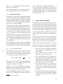
Modeling flow
The flow of files and operations when modeling
with ASPIC and related programs is summarized in
Fig. 1 on page 8. It may be helpful to refer to Fig. 1
as you read this manual.
4.2
Data on fishing effort rate can be used instead of
relative abundance, and if so, they are assumed to
represent effective (standardized) effort. This implies that effort divided by yield forms an unbiased
index of the stock’s relative abundance.
In this User’s Guide, the terms “catch” and “yield”
are used interchangeably to mean total removals
in biomass. Similarly, CPUE is used to mean some
index of relative abundance. The presumption is
that the CPUE has been standardized before being
used for modeling.
In addition to data, ASPIC requires starting guesses
of its estimated parameters. The leading parameters are—
User Interface
• MSY (maximum sustainable yield)
• FMSY (fishing mortality rate under which MSY
can be attained)
• B1 /K (ratio of stock biomass at the beginning of the analysis to K, the carrying capacity)5
• For each data series, indexed by j = 1, . . . , J,
the catchability coefficient qj .
This section assumes that the user has installed
ASPIC successfully with the Windows installer. The
Linux version of ASPIC, when available, has a similar
interface to the Windows version.
ASPIC does not include the graphical user interface
that is typical of commercial software. It is a textmode program that reads input from text files and
write output to new text files. While running, it
may prints informational or error messages to the
console (screen). After the program completes or
aborts an analysis, it must be started again to run
a new analysis.
V
The program is supplied in two variants, which are
computationally identical. Program aspic7.exe
runs in any standard Windows console (command
window). The other variant, aspic7g.exe, runs in
its own graphical console, which stays open so the
user can scroll through any screen output. The
ASPIC shortcut (icon) starts aspic7g.exe, which is
more suited to drag-and-drop of input files.
4.3
A full description of the input file format is given in
§5 and includes suggestions for starting guesses.
The starting guess for each parameter also must
include bounds (minimum and maximum values of
the parameter), and in MAP estimation, the prior
distribution and its parameters.
4.4
4. Production models also have been used successfully with
data on removals in numbers.
Program limits
Current programs limits are as follows:
Years of data: 150
Number of data series: 12
Bootstrap trials: 3000
Time steps/year in numerical integration of
generalized model: 100
• Years of projection (ASPICP): 100
•
•
•
•
Data requirements
Data needed by ASPIC are a series of observations
on yield (catch in biomass)4 and one or more corresponding series of relative abundance. ASPIC assumes that the supplied abundance index is an
unbiased index of the stock’s abundance in biomass.
V
Any user with larger requirements is invited to
contact the author.
4.5
Program modes
ASPIC has two modes of operation, or program
modes:
5.
K is equivalent to the unfished biomass.
7
V
V
Figure 1: Modeling flow with ASPIC Suite.
Fitting step
Start
Bootstrap step
(uncertainty)
2
No
Make/edit
.a7inp file *
Run ASPIC
(FIT mode)
.fit file **
OK?
Yes
2
.bot file **
Modify
.a7inp file *
Run ASPIC
(BOT mode)
3
.bio file
Projection step
3
Make/edit
.ctl file *
Run ASPICP
.prj file **
Do more
projections?
Yes
Files marked * are human viewable. Files
marked ** are viewable and also graphable
with AGRAPH.
8
No
End
• In FIT mode, ASPIC fits the model and computes estimates of parameters and other
quantities of management interest, including time trajectories of fishing intensity and
stock biomass. Execution time is relatively
short.
• In BOT mode, ASPIC fits the model and computes bootstrapped confidence intervals on
estimated quantities. Because computations
are extensive, execution time in BOT mode is
considerably longer than in FIT mode. For
example, a bootstrap with 500 trials might
take 500 times as long as a single fit.
A typical analysis begins using FIT mode, and making several runs to explore different model structures. After model and data structure have been
decided—and it is established that parameter estimates can be obtained—BOT mode can be used to
estimate uncertainty in results (Fig. 1).
Previous versions of ASPIC had a third program
mode, for iterative reweighting of data series. That
mode is no longer available.
4.6
Fitting more than one data series
ASPIC can fit data on up to 12 simultaneous or serial
fisheries (biomass estimate series or biomass index
series). Data series may be of several types (Table 1),
but at least one series must be type CE (effort and
yield) or type CC (CPUE and yield). When more than
one series is analyzed, common estimates of B1 /K,
MSY, and FMSY are made, along with an estimate of
qj for each series. The interpretation of qj depends
on the type of data series that it describes.
A statistical weight wj for each data series is specified by the user in the input file, and the weights
are normalized by the program so that they sum to
unity. The use of the weights varies slightly for the
different objective functions. See §8 for details.
The computer time needed to obtain estimates generally increases as more data series are added. The
increase is due to both the added data and the
increased difficulty of optimization.
4.7
Choices for fitting
4.7.1 Estimation methods
ASPIC is a continuous-time, observation-error estimator that assumes observation errors are lognormally distributed. Four methods of estimation
are provided: least squares, least absolute values,
maximum likelihood, and maximum a posteriori.
Estimation modes are described on p. 14, and technical details are given in §8.1.
4.7.2 Statistical conditioning
ASPIC can consider yield known exactly and accumulate residuals in effort or relative abundance; it
can also do the reverse. Specifying this option is
covered on p. 13. Whichever quantity is chosen for
conditioning must be free of missing values in the
input data.
Yield usually is known more precisely than effort
or relative abundance; therefore, conditioning on
yield is recommended for most analyses. When
conditioning on yield, an iterative solution of the
catch equation is used, and computation is slower
than when conditioning on fishing effort.
4.7.3 Penalty for B1 > K
A penalty can be added to the objective function
to discourage estimates in which the first year’s
biomass B1 is greater than the carrying capacity
K. This penalty can affect the estimates of other
parameters, so when the penalty is nonzero, results
should be compared to those obtained without the
penalty or by fixing the initial biomass at several
plausible fractions of K. The penalty term is described in more detail in Prager (1994); its specification is described on p. 15; technical details are
given in subsections of §8.
4.7.4 Residuals and bootstrapping
In bootstrap program mode, saved residuals are
multiplied by an inflation factor (Stine 1990, p. 338),
reported in the output file. The factor is described
in §8.6.3.
A resampled data set is then generated by combining each saved predicted datum with a randomly9
Table 1: Codes for the eight types of data series allowed in ASPIC.
Code
Data type
When measured
CE
Fishing effort rate and yield
CC
CPUE and catch
B0
B1
B2
I0
I1
I2
Estimate of biomass
Estimate of biomass
Estimate of biomass
Index of biomass
Index of biomass
Index of biomass
Effort rate: annual average
Catch: annual total
CPUE: annual average
Catch: annual total
Start of year
Annual average
End of year
Start of year
Annual average
End of year
chosen residual. The model is then refit to the resampled data. The process is repeated (always using the original predicted values) up to 3,000 times.
The author recommends using at least 500 bootstrap trials to calculate the ASPIC’s default 80%
confidence intervals. More trials should be used
for wider intervals, to ensure that the tails of the
distribution are better defined.
Some bootstrap trials may produce parameter estimates at or outside the user’s specified bounds.
Such trials are discarded automatically and replaced by new trials. A report on discarded trials is
part of the main output file.
4.8
Input and output files
All ASPIC input and output files (Table 2) are in
plain ASCII format. Numerous sample files are included in the ASPIC distribution.
this work: the ability to cut and paste rectangular
blocks of text (such as data columns). An excellent,
free editor for general use is Notepad++, which as
of May, 2014, was easily found with a Web search
engine.
4.8.2 Output files
ASPIC produces several output files. Although all
are written in plain ASCII, some are meant for human readability and others for use by ancillary
programs. The main .fit and .bot output files,
like all the files meant to be read by the user, have
line lengths of 120 characters or less. Files meant
for ancillary programs may have longer lines.
Names of output files are constructed from the root
file name of the run’s input file, with the appropriate file extension appended (Table 2). The following
paragraphs summarize the types of output files
generated by ASPIC:
4.8.1 Input file
An ASPIC input file contains all data and settings
required for a single ASPIC run. The simplest way
to make an ASPIC input file is to copy one of the
sample files and edit it with your own data and
specifications. The input file format is given in full
detail in §5.
A text editor6 is needed for editing ASPIC input files.
One possibility is Windows Notepad, included with
every copy of Windows. Unfortunately, Notepad is
a rudimentary editor that lacks a key feature for
6.
10
Text editors are also known as programming editors.
u Main output files. The file extension of the
main output file depends on program mode (Table 2). Suppose the input file is sword.inp. In FIT
mode, the main output file will be sword.fit; in
BOT mode, it will be sword.bot.
The main ASPIC output file includes parameter estimates; measures of goodness of fit; and estimates
of population benchmarks, biomass levels, and exploitation levels, as well as simple character plots.
Output from bootstrap runs also includes confidence intervals on many estimated quantities.
Table 2: Input (I) and output (O) files of ASPIC and related programs.
File
extension
.a7inp
‡
†
Input or
output?
Used
by
File contents and description
I
ASPIC
Input file with data, starting guesses, and run settings
ASPIC
ASPIC
ASPIC, ASPICP
Main output file from FIT program mode
Main output file from BOT program mode
Estimated B and F trajectory for each bootstrap trial (BOT program mode); used by ASPICP.
Estimates from each bootstrap trial (BOT program mode).
Optional file with summary of all runs made in a directory
.fit‡
.bot‡
.bio†
O
O
O, I
.det†
.sum
O
O
ASPIC
ASPIC
.prn
O
ASPIC
.rdat†
O
ASPIC
.rdatb†
.gen
O
O
ASPIC
ASPIC
.ctl
.prj‡
.prb
.rdat†
I
O
O
O
ASPICP
ASPICP
ASPICP
ASPICP
Estimated trajectories in a table easily read by a spreadsheet or
statistics program
Detailed output file formatted for reading by the dget() function
of R. Includes inputs and estimates.
As above, but from bootstrap runs
Summary results from GENGRID mode
Control file with projection parameters
Projection results
Supplement of .bio file with projection results
Detailed output file of projection, formatted for reading by the
dget() function of R
File types readable by AGRAPH .
File types intended for reading mainly by other computer programs.
u Bootstrap-related files. Two additional files are
generated after bootstrap runs to allow further data
analysis. The .bio file is used by ASPICP (described
below) for projections following a bootstrap run.
The .det file provides information on the individual bootstrap trials. It is not used directly by any
supplied program, but it can be useful in further
analysis.
u Simple R or spreadsheet output. A file with extension .prn and containing a table of time-series
estimates can be output from an ASPIC run. The
file is meant to be compatible with such programs
as R, SAS, and spreadsheets. To enable this file, see
specification of verbosity on p. 13. If you are using
R for, the more complete .rdat file, described next,
is preferred.
u Detailed R-compatible output. More complete
R-compatible output is available from ASPIC runs
through a file with extension .rdat (FIT mode) or
.rdatb (BOT mode). Either file can be read by R
to generate a data object of type “list”, containing
extensive results from the run. For example in R,
sword <- dget("sword.rdat")
The section on specification of verbosity (p. 13) describes how to enable output of these files.
u Summary of multiple runs. To aid in simulation
studies, a summary file (.sum file) can be written in
the current directory. Again, the verbosity setting
in the input file (p. 13) determines whether this file
is written. The .sum file can be read by and most
spreadsheets and statistics packages. It can be R
with a statement like
mydata <- read.table("aspic.sum",
header = TRUE)
4.9
Running ASPIC
First prepare an input file in the correct format (§5
on page 12). It’s easiest to copy one of the sample
input files provided to use as a template.
11
Then start the program, giving the input file name
on the command line.For example, the command
aspic7 sword.a7inp
will cause the program to read an input file
named sword.a7inp and produce corresponding
estimates and output files. If only the command
aspic7
is given, the program looks for the default input
file, aspic.a7inp.
If the .sum file as been enabled, summary output
from each run in the directory will be written to
it. The default name is aspic.sum. To use a different name for the .sum file, give the name on the
command line. For example, the command
aspic7 sword.a7inp mysum
will read the file sword.a7inp and create (or write
to) the summary file mysum.sum, along with other
ASPIC output.
To use drag-and-drop instead of the command line,
simply drag the icon of an ASPIC 7 input file (extension .a7inp) to the shortcut for ASPIC 7 created by
the installer.7 The ASPIC Quick Reference, installed
with the ASPIC Suite, includes more information on
drag-and-drop use.
Severe errors detected while ASPIC is reading the
input file will cause the program to print a descriptive message and stop. If the message is not clear,
comparing the input file to the samples provided
may reveal format errors.
5
ASPIC 7 input file specification
ASPIC 7 takes its input from a single file containing
control parameters and data. The format of that
file is described in this section.
V
The input file format has changed. The utility program ASPIC5to7 (§6.1) can be used to convert ASPIC
5 input files to the new format.
5.1
Data representations
Data in the input file must be represented in specific ways.
V
• Any line after line 1 can be a comment. A
7.
12
The shortcut points to aspic7g.exe.
comment must have the hash character (#)
in column 1. Comments are ignored by the
program.
• Data values are not required to be in specific
columns of the line. If a line contains more
than one value, however, they must be in the
correct order.
• Values on a line should be separated by
spaces (blanks). Using tab characters to separate values is not guaranteed to work.
The remaining format rules depend upon the type
of the data item (integer, real, or character).
• Each real number must contain a decimal
point, an exponent (denoted by the letter
d or e), or both a decimal point and an exponent. Examples: 1.0, 2e3, 1.3d6. (Note
that 2e3 means 2 × 103 .) An integer may be
used in place of a whole real number.
• Integers must not contain decimal points
or exponents. Examples: 0, 2, 94541. The
value 1.0 is not valid when an integer is
required
• Character strings may be quoted, i. e., enclosed in matched apostrophes or quotation
marks. Quoting is optional unless the string
contains blanks or other special characters.
Here are three examples of valid character
strings:
FallIndex
'This is a valid string'
"Another valid string"
• Each line must have the specified number of
values, separated by spaces. Values may not
be otherwise arranged among lines.
• After all required values have been read
from a line, the program does not read further. Thus, the rest of the line may be used as
a comment. End-of-line comments in sample
input files are sometimes preceded by hash
characters, ##. The hash characters are used
to make the comments stand out and are
not required before end-of-line comments.
• After all data have been read from the file,
as determined by the number of years of
data and number of data series, any further
contents of the file are ignored by ASPIC.
Thus, additional comments may be placed
at the end of the file.
5.2
Line-by-line details
Here, each line of the input file is explained in detail.
Comments may appear almost anywhere, so line
numbers given here exclude comments inserted by
the user.
Line 1: Version indicator
Each ASPIC 7 input file must contain the following
ID string on line 1:
ASPIC-V7
* Comments are not allowed before the ID string.
Line 2: Run title
The run title is a character string of up to 110
characters. This title is written to the main output
file to identify the analysis. It will also appear on
graphs made with AGRAPH and projections made
with ASPICP.
Since the run title typically contains spaces, it
should be quoted. For example:
"Run 4 for Swordfish, 1994"
Line 3: Program mode, verbosity, & bootstrap
Line 3 contains up to four values controlling basic
features of the program’s execution.
Ê The first value on line 3 is the program mode, a
character string of length 3. Possible values are FIT
(fitting mode) or BOT (bootstrap mode). Program
modes were described in §4.5 on page 7.
Ë The second value on line 3 is the verbosity, an
integer controlling the amount of screen output
during the run. It also controls whether optional
.sum, .prn, and .rdat files (§4.8) are generated.
Screen output is controlled by setting verbosity
between 0 and 4. Using 0 gives almost no screen
output; 2, moderate output; and 4, extensive output meant for debugging the program. The recommended default is 2.
To generate .sum and .prn files, add 10 to the verbosity. For example, verbosity of 12 generates those
files and gives moderate screen output.
To generate an R-compatible .rdat file, add 100 to
the verbosity. For example, 112 generates all optional files and moderate screen output. Verbosity
of 102 generates an .rdat file and moderate screen
output.
To avoid the usual prompt when an output file
is about to be overwritten, use verbosity of 0 or
change the sign of a positive verbosity. In that case,
ASPIC will overwrite an output file without asking,
which can be useful when ASPIC is run by a script
or another program.
Ì The third value on line 3 is the number of bootstraps, an integer up to 3000. In FIT mode, this
value may be omitted. If present, it is ignored.
Í The fourth value on line 3 is an optional integer
30 ≤ n2 ≤ 95, used to set the width of confidence
intervals (CIs) in bootstrap mode. ASPIC provides
two sets of confidence intervals: The first are always
80% confidence intervals, and the second are 50%
intervals by default, e. g., when n2 is omitted. To
replace 50% CIs with 75% CIs (for example), set
n2 to 75. Wider intervals require more bootstrap
trials to compute precisely. The author suggests
that when n2 > 80, the number of bootstraps trials
be between 1000 and 3000.
Line 4: Model shape, conditioning, & estimation
mode
Line 4 has three specifications controlling model
form and fitting.
Ê The first value on line 4 is a character string
specifying model shape.
Value
Meaning
LOGISTIC
GENGRID
Fit the logistic (Schaefer) model.
Fit the generalized (Pella–Tomlinson)
model at a grid of values
Fit the Fox model (a special case of
GENFIT, below).
Fit the generalized model and estimate its exponent directly.
FOX
GENFIT
Ë The second value on line 4 is a character string
specifying statistical conditioning in estimation. For
more information, see §4.7.2.
13
Value
Meaning
YLD
Condition on yield (recommended for most
analyses).
Condition on fishing effort rate
EFT
Ì The third value on line 4 is a character string
specifying the estimation method.
Value
Estimation method
SSE
LAV
MLE
MAP
Least squares
Least absolute values
Maximum likelihood
Maximum a posteriori—a form of penalized likelihood using Bayesian priors.
The first two estimation methods were available in
ASPIC 5; the last two are new in ASPIC 7. Annual
CVs on observations can be accommodated by MLE
and MAP estimation.
Line 5: Data extents
Line 5 holds two integer values.
Ê The first value on line 5 is an integer specifying
the length of (number of years in) each data series.
The maximum value is 150.
Ë The second value on line 5 is an integer specifying the number of data series in the file. The
maximum value is 12.
Line 6: Monte Carlo searching
This line contains two integers to control the optional Monte Carlo (MC) search during fitting.
Ê The first value on line 6 sets the MC search mode
(intensity). The value may be 0 to disable Monte
Carlo searching; 1 to enable basic MC searching; or
2 for repeated searching.
present, a MC search occasionally leads to one of
them. Thus, it can be better to use MC searching
as needed, rather than routinely. When needed, a
reasonable pair of MC settings is 1 100000. The
number of trials would be increased or decreased,
depending on the difficulty of the problem and the
speed of the computer.
Monte Carlo searching can increase execution time
considerably, especially when repeated searching
is enabled during a bootstrap. For that reason, increasing the number of searches may be more useful than using mode 2 in a bootstrap run.
Line 7: Convergence criteria
Line 7 holds three real numbers controlling convergence in optimization. The suggested values have
been chosen through much experience. Users are
not encouraged to change them without reason. In
cases where a fit is difficult to obtain, it might be
helpful to reduce them each by one power of ten.
Ê The first number, ε1 , is the convergence tolerance
of the Nelder–Mead optimizer among its several
trial parameter vectors. After each adjustment, the
objective function is computed for each set of trial
values. Convergence is defined to occur when the
following condition is met:
2 |Oα − Oω |
< ε1 .
Oα + O ω
where Oα is the best objective-function value in the
polytope and Oω is the worst.
The recommended value is ε1 = 1 × 10−8 , which
is written as 1d-8 in the input file. Changing this
value is not recommended.
Ë The second value on line 6 sets the number of
Monte Carlo trials. When repeated searching (mode
2) is selected, the number of trials in searches after
the first is reduced by 1/3. A value is required, even
when Monte Carlo intensity is 0.
Ë The second number is ε2 , the convergence tolerance of randomized restarts, which are used by
ASPIC to escape local minima. When objective function values from k consecutive starts agree within
this tolerance, the solution is accepted. (The value
of k is set on the following line.) The recommended
value is ε2 = 3 × 10−8 , which is written as 3d-8
in the input file. Changing this value is not recommended.
Comments: Search modes 1 and 2 can be helpful
when a repeatable solution is otherwise difficult to
find. Unfortunately, when strong local minima are
Ì The third value is the convergence tolerance ε3
in computing fishing mortality when conditioning
on yield. The approximation stops when successive
14
estimates of F are within ε3 . The recommended
value is ε3 = 1 × 10−4 , which is written as 1.0d-4
in the input file.
In EFT conditioning mode, the value of ε3 is not
used, but a value must be present nonetheless.
Line 10: Initialization of B1 /K
Line 10 is the first of several lines with values that
control estimation of the model’s parameters. This
line controls the ratio B1 /K, where B1 is the biomass at the start of the first year, and K is the
carrying capacity.
Line 8: Computational parameters
Ê Line 10 must start with the character string B1K.
Line 8 holds three additional values controlling
computation and fitting.
Ë The second value on line 10 is a starting guess for
B1 /K, typically a real number between zero and one.
Ideally, this is based on knowledge of the stock’s
condition at the start of the data set. Absent such
information, a reasonable default is 0.5.
Ê The first value on line 8 is F∞ , a real number specifying maximum estimated F when conditioning on
yield. The recommended default, 8.0d0, works well
in many cases. This value is used to guide the optimizer, and reducing the value may cause estimation
problems.
* If F∞ is less than the maximum bound set on
FMSY below, it acts as a more restrictive maximum
bound on FMSY . In other words, F∞ can override the
user’s maximum on FMSY .
Ë The second value on line 8 is the integer k, the
number of consecutive restarts required for accepting parameter estimates. The recommended default
is 8. A larger k should be used when there are more
than 2 data series or when reaching a good answer
seems difficult. In rare cases where fitting is extremely difficult, a much larger number (say, 64)
could be tried.
Ì The third value on line 8 is integer n, the number
of time steps per year in approximating the generalized production model. Allowable values are
between 2 and 100; suggested values are between
6 and 24. Larger n causes slower execution.
* When fitting the logistic model, a value of n need
not be present. If present, it is ignored.
Line 9: Random number seed
Line 9 holds one value, a seed for initializing the
random-number generator. This should be a large
(7-digit) positive integer. Different seeds result in
different random number sequences; using the
same seed allows duplicating a previous run.8
8. See §7.3 for advice on estimation sensitivity to choice of
seed.
Ì The third value on line 10 is the estimation flag,
an integer: 1 to estimate B1 /K, or 0 to use the starting guess as a fixed value.
* If the estimation flag is 0, no further values are
required on this line. If present, they are ignored.
When the estimation flag is 1, additional values are
required—
Í–Î The fourth and fifth values on line 10 are two
real numbers: lower and upper bounds on the estimate of B1 /K. Only values within those bounds will
be examined by the optimizer in point estimation
and in bootstrapping.
* The following values on this line differ, depending on whether MAP estimation is being used.
With other than MAP estimation—
When using estimation methods SSE, LAV, or MLE,
the remaining values on line 10 specify a penalty
b > 1.
added to the objective function when Bb1 /K
Ï The sixth value on the line is the character
string penalty.
Ð The seventh value is a real number, the statistical weight of the penalty term. For no
penalty, enter 0.0. To use a penalty, enter a
positive real number, typically 1.0.
The penalty is useful in analyses showing a sharp
decline in abundance in the initial years; such patterns can otherwise result in an extremely high
estimate of B1 .
The recommended default is 0.0 (no penalty). If
the resulting estimate of B1 /K is too high, the analyst can try either a nonzero penalty or fixing
15
4
B1 /K rather than estimating it. Either approach can
affect estimates of management quantities; sensitivity analyses are useful to examine this.
The penalty term is described in Prager (1994); fixing B1 , in Punt (1990). Mathematical details of the
penalty’s application in ASPIC 7 are given in §8.2.2
and sections following it.
“Geometry of the probability distribution function.”)
Examples of line 10
z B1 /K fixed at starting value of 0.75:
B1K
0.75
0
z Other than MAP estimation; penalty enabled:
With MAP estimation (prior specification)—
4
When using MAP, the remaining values on this line
specify the prior distribution for B1 /K.
Ï The sixth value is the character string prior.
Ð The seventh value is a character string
giving the name of the prior distribution.
This may be uniform, normal, lognormal,
triangular, or beta.
Ñ The eighth and following values are real
numbers giving parameters of the chosen
prior distribution—
– For the uniform distribution, two values: lower bound and upper bound.
– For the normal distribution, two values:
the mean and coefficient of variation,
cv = σ /µ, where σ is the standard deviation and µ the mean.
– For the lognormal distribution, two values: the distribution’s mode and the
standard deviation of the logged distribution. (The second parameter is approximately equal to the c. v. of the distribution.)
– For the triangular distribution, three
values: the lower bound, the value at
peak probability density, and the upper
bound.
– For the beta distribution, four values: shape parameters α and β, then
lower and upper bounds. (The standard
beta distribution is supported on [0, 1].
Here, it is scaled to the range between
the user’s lower and upper bounds.)
For more information on possible
shapes of the beta distribution, the user
might consult a text on statistical distributions, or even the relevant Wikipedia
page, in particular, the section titled
16
B1K
0.9
1
0.1
5.0 penalty 1.0
z Other than MAP estimation, penalty disabled:
B1K
0.5
1
0.1
5.0 penalty 0.0
z MAP estimation with uniform prior:
B1K 0.9
1
0.2 1.5
prior uniform 0.2 1.5
z MAP estimation with beta prior:
B1K 0.5 1
0.1 2.0
prior beta 2.0 2.0 0.1 2.0
Line 11: Initialization of MSY
Line 11 controls estimation of MSY.
Ê The first value on line 11 is character string MSY.
Ë The second number is a real number, the user’s
starting guess of MSY. In the absence of other information, 80% of the largest observed yield can be
a reasonable default. See also §7.1 on page 22.
Ì The third number is the integer estimation flag:
1 to estimate MSY or 0 to use the starting guess as
a fixed value.
* If the estimation flag is 0, no further values are
required, and if present, they are ignored. When the
estimation flag is 1, additional values are required—
Í–Î Two real numbers: lower and upper bounds
on MSY.
* Further values are required only when using MAP
estimation.
Ï+ The character string prior; the name of the
prior distribution on MSY; and two to four real
numbers, parameters of the distribution. [See text
on initialization of B1 /K (p. 16) for a more detailed
description of specifying prior distributions.]
* ASPIC includes logic that prevents MSY from
exceeding the carrying capacity K. If your analysis
requires MSY > K, you can divide your annual input
data into two or more periods per year, and MSY
on a per-period basis will be reduced accordingly.
Population parameter K does not have time units
and would be unaffected.
ignored. Nonetheless, a properly formatted line for
each of the J data series is required.
Each line is similar to preceding lines:
Ê The character q.
Examples of line 11
Ë A real number, the starting guess for qj .
z When not using MAP optimization:
Ì The integer 1 to estimate qj , or 0 to use the
starting guess as a fixed value.
MSY 1.2d3
1
400.0 1d4
Í A real number: statistical weight of this series
in the objective function. Suggested default is 1.0.
(Use of these weights is described in §8.)
or
MSY 1.2d3
0
z When using MAP optimization:
MSY 1d3 1
1d2 1d4
prior lognormal 1d3 0.2
Line 12: Initialization of FMSY
Line 12 controls estimation of FMSY , using the same
format as the preceding line.
Ê The character string FMSY.
Ë A real number, the starting guess for FMSY .
Ì The integer (estimation flag) 1 to estimate FMSY
or 0 to use the starting guess as a fixed value.
* If the estimation flag is 0, no further entries are
required on this line. If present, they are ignored.
Í–Î Two real numbers: lower and upper bounds
on FMSY .
* If the estimation flag is 0, no further entries are
required on this line. If present, they are ignored.
ΖΠTwo real numbers giving lower and upper
bounds on qj .
Ð. . . When using MAP optimization and estimating qj , the prior specification: The character string
prior; the name of the prior distribution on qj ; and
two to four real numbers, parameters of that distribution. See text on initialization of B1 /K (p. 16) for
details on specifying priors.
Examples of q specification lines
z For a biomass series (B0, B1, or B2):
q
1.0
0
1.0
z When not using MAP optimization:
* Further entries are required on this line only
when using MAP estimation.
q
Ï+ The character string prior; the name of the
prior distribution on FMSY ; and two to four real
numbers, parameters of the prior distribution. See
text on initialization of B1 /K (p. 16) for details on
specification of priors.
q 0.1 1 1.0 0.02 0.9
Lines 13 and following: Initialization of q
The next lines control estimation of the catchability
coefficients qj , where j = {1, 2, . . . , J} denotes the
data series. One line is required for each data series
in the input file, in the same order that the data
series appear in the file.
In data series of types B0, B1, and B2, q = 1 by
definition, and thus most data on the line will be
0.1
1
1.0
0.02
0.9
z When using MAP optimization:
prior normal 0.1 0.5
Next line: Initialization of model shape φ
The next line controls estimation of the shape parameter in the generalized model. In ASPIC, shape
is represented by φ = BMSY /K, a fraction in (0, 1).
* This line is needed only when model shape
choice on line 4 is GENGRID or GENFIT. A line beginning with the required string POS will be ignored if
another model shape is specified.
* Some contents of this line vary by model shape
specification.
u
If using GENFIT model shape:
17
Ê The character string POS or pos.
Ë An integer, the starting guess for 100 · φ. (For
example, if the guess for φ is 0.4, enter 40 here.
Ì An integer, 1 to estimate φ or 0 to use the starting guess as a fixed value.
* If the estimation flag is 0, no further entries are
required on this line.
Í-Î Two integers: lower and upper bounds on 100·
φ.
Ï A real number ξ to bound the generalized estimates with respect to the logistic estimates.9 For
example, 8.0 means that MSY for the generalized
fit will be bounded between 1/8 of and 8 times
MSY estimated by the logistic fit and that FMSY will
be bounded similarly. A change is made only if it
results in a stricter bound than the explicit bound
set by the user.
In a bootstrap run, bounds changes are in effect
only for the initial fit of the generalized model. In
bootstrap trials, the user’s bounds are restored.
If the user specifies ξ = 0.0, no bounds changes are
made. When ξ > 0, ASPIC requires that ξ ≥ 3.0. In
studies so far, ξ = 8.0 has worked well.
Ð. . . When using MAP optimization and estimating φ, the prior specification: The character string
prior; the name of the prior distribution on φ; and
two to four real numbers, parameters of that distribution. See text on initialization of B1 /K (p. 16) for
details on specifying priors. Prior parameters on φ
are given as real numbers on the scale of φ, not as
integers.
Examples of φ specification with GENFIT:
z When no prior is used:
pos 40
1
30 75 8.0
z When a prior is used (MAP estimation):
pos 40 1 30 75 8.0 prior normal 0.4 0.3
u If using GENGRID model shape:
Ê The character string POS.
9. When fitting the generalized model, ASPIC always fits the
logistic model first, to improve starting values.
18
Ë An integer: the minimum value of 100 · φ for the
grid search.
Ì An integer: the maximum value of 100 · φ for
the grid search.
Í An integer: the step size of 100 · φ in the grid
search.
Î A real number ξ bounding the generalized estimates near the logistic estimates. A full description
is in the preceding section on inputs for GENFIT
operation.
Ï+ If a prior is used, its specification, in the same
format described for GENFIT operation.
Examples of φ specification with GENGRID:
z When no prior is used:
pos
40
25
85
5
8.0
z When a prior is used:
pos 40 25 85 5 8.0 prior normal 0.45 0.25
Next line: Marker for start of data
This line should contain the character string DATA.
Following lines: Individual data series
There must be one data block (group of lines) for
each data series. Each block must include data for
all y years; thus, each data block is the same length
y. The composition of each block is as follows—
(a) On the first line of the block, a series title
(character, length ≤ 40, in quotes). Example:
''Spring survey & total landings''
(b) On the second line of the block, a character
string of length 2 with the type code for the
series. Type codes are listed in Table 1 (p.
10).
(c) Starting on the third line of the block, one
data line for each year, with the following
data on each line, separated by blanks —
(c1) First number — the year or other ID
number. These integers must be consecutive, less than 9999, and identical
from block (data series) to block.
(c2) Second number — a real number whose
meaning depends on the series type:
For type CE, the fishing-effort rate f for
the year; for types CC or I1, the average
relative abundance; for types I0 or I2,
the relative abundance near the start or
end of the year; for types B0, B1, or B2,
the stock-biomass estimate.
(c3) Third number — a real number, required in CE or CC series only, giving
yield for that year. Please see §7.2.3
for advice on allocating yield among
data series. This number must not be
present in Bn or In data series.
(c4) Final number — an additional real number, required only when the estimation
option is MSE or MAP. In those cases, it
is the c.v. of the data point. With other
estimation options, the c.v. is ignored.
* Although yield–effort data series are designated
type CE, effort is entered before yield on these lines.
Similarly, in series type CC, the relative abundance
appears before the yield.
V
6
Auxiliary Programs
6.1
ASPIC5to7
ASPIC5to7 is a utility program to convert input
files from ASPIC 5 to ASPIC 7 format. A new file
is written with extension .a7inp, and the existing
input file (extension .inp) is not changed.
Like ASPIC, ASPIC5to7 is a text-mode program.
Also like ASPIC, it is supplied in two variants:
aspic5to7.exe for use from the command line,
and aspic5to7g, for use with drag and drop.
For drag and drop operation, simply drag the
icon of a valid ASPIC 5 input file to the icon for
ASPIC5to7.10 An ASPIC 7 input file will be generated, and a display window will be opened to show
the results of the conversion. This then should be
closed by the user.
For command-line operation, simply enter the program name and name of the existing ASPIC 5.x input
file. For example, the command
aspic5to7 sword.inp
10. The installed icon is labeled ASPIC5to7, but it runs
aspic5to7g.exe.
will generate sword.a7inp. By default, the new file
will contain comments to make it easier to read.
To avoid this, use program option -nocomments,
which may be shortened to -nocom. For example
aspic5to7 sword.inp -nocom
generates a new file without comments.
To change the operation of the installed shortcut
so that generated files do not include comments,
edit its properties and insert the option.
6.2
AGRAPH
The Windows program AGRAPH is intended to provide quick, legible graphics of ASPIC and ASPICP
results.
AGRAPH can process files from ASPIC with .fit or
.bot extensions and from ASPICP with .prj extension. The plots from .fit and .bot files include
time-series of relative benchmarks and plots of
observed and fitted abundance indices. For benchmark plots with confidence intervals, run a bootstrap, then a projection with ASPICP, and send the
resulting .prj file to AGRAPH.
AGRAPH is not intended to meet all graphics needs
of ASPIC users. It allows examining results quickly
and supplies standard graphics for reports. For
more advanced graphics, a spreadsheet or statistics
program can be used, taking advantage of specialized ASPIC output files (§4.8).
This is the only program in the ASPIC Suite that
incorporates a standard Windows GUI, with output
available to any Windows printer, to a graphics file
(WMF or EPS), or to the Windows clipboard.
Operation of AGRAPH is similar to that of any Windows program. It can be opened in three ways
• By clicking on its icon, then choosing a file
for analysis
• By dragging a suitable file to the AGRAPH
icon
• From the Windows command line
As a command-line example,
agraph sword.fit
will open file file sword.fit and display a graph of
the results.
19
AGRAPH contains a brief help screen that explains
its menu items.
6.3
ASPICP
After an ASPIC boostrap run, ASPICP calculates bootstrap confidence intervals on the estimated trajectories of population biomass and fishing mortality,
both for the assessment period and for a projection
period of up to 100 years.11 One projection trial is
made for each bootstrap trial in the original ASPIC
run.
For technical information on ASPICP projections,
see §8.7.
ASPICP output (.prj) files can be read by AGRAPH
to make time plots of B/BMSY and F /FMSY with bootstrap confidence intervals.
6.3.1 ASPICP interface and use
The interface of ASPICP is similar to that of ASPIC:
a text-mode program that reads from and writes
to plain-text files. The program is supplied in two
computationally identical variants: aspicp5.exe
for use from the command line, and aspicp5g.exe
for drag-and-drop.
ASPICP reads the user’s projection specifications
from a control file, which must have file extension
ctl. The control file (among other things) gives
the name of the .bio file from an ASPIC bootstrap
run, from which bootstrap estimates of FMSY , BMSY ,
annual B, and annual F are read.
The contents of an ASPICP control file are explained
in the following section, and several sample files are
included in the ASPIC distribution. Control files are
created and edited with a text editor (programming
editor).12
To run ASPICP, either drag and drop a .ctl file to
the ASPICP shortcut13 or use the command line. For
example, the command
aspicp5 snapper.ctl
11. Long-term projections are useful only in a statistical sense.
They are provided in ASPICP for use in an educational setting,
to enable demonstrations of theoretical population properties
under various management schemes.
12. The discussion of editors in §4.8.1 applies here.
13. The installed shortcut points to aspicp5g.exe
20
starts ASPICP and runs a projection as described in
control file snapper.ctl.
The main ASPICP output report is written to a file
with extension prj. More detailed results from projection trials are in a file with extension prb, an
extension of the .bio file (Table 2) that includes
projection years. The .prb file is meant for analysis
with a statistics program or spreadsheet.
6.3.2 ASPICP control file specification
The control file for ASPICP is relatively short. For
allowed representations of real, character, and integer data, please see §5.1.
The top portion of the control file does not allow
full-line comments, but end-of-line comments are
allowed. Any text following the required values on
a line is treated as a comment.
The current version of the ASPICP control file has
more features and flexibility than previous versions.
The program will read older .ctl files,14 but the
new format is preferred.
Line 1: ID string
Each ASPICP input file in new format must contain
the following character string on line 1:
ASPICP-V4
Line 2: Projection title
This is a character string, length ≤ 100. A title
that includes blanks (spaces) must be enclosed in
quotation marks. The ASPICP output file includes
this title and the title of the original ASPIC run.
* The graphics library in AGRAPH uses the asterisk
character (*) as an escape. If you will graph your
projection results with AGRAPH, avoid using the
asterisk in this title.
Example:
"Projection of swordfish at Fmsy"
14. The older format is given in the ASPIC 5 User’s Guide
V
Line 3: Name of .bio file
A character string specifying the name of a .bio
file from an ASPIC bootstrap run. If the filename
contains blanks, it must be quoted.
Example:
redporgy.bio
V
Line 4: CV of MSY during projection
This is a real value from 0.0 to 1.0 that sets an
additional CV on MSY during projections. Typical
values range from 0.0 to 0.5. See §8.7.1 for details
of how this number is used.
Line 5: Confidence interval control
Ê The first value on line 5 is a two-letter character string that sets the type of confidence interval
used. This may be BC for bias-corrected confidence
intervals (Efron and Gong 1983), or PC for simple
percentile confidence intervals. The latter may be
preferable when the BC intervals appear irregular,
which can occur on some data sets.
Ë The second value on line 5 is an integer, 1 to
smooth the confidence intervals or 0 to use unsmoothed results. Smoothing, a heuristic measure
to improve regularity of the intervals, was the default in older versions of ASPICP. Using smoothing
is recommended when using BC intervals.
Example:
Ê The first flag determines whether AGRAPH should
open automatically at the end of projections to plot
the results.
Ë The second flag determines whether a .prb file
is written. This detailed output file can be read
by a statistics package or spreadsheet to analyze
projection results.
Ì The third flag determines whether an .rdat (Rcompatible) output file should be written. This is a
version of the main output file (.prj file) that can
be read by R with its dget function.
Line 8: Random number seed
Line 8 holds one value, a seed for initializing the
random-number generator.15 This entry is a large
(7-digit) positive integer. Different seeds result in
different random number sequences; using the
same seed allows duplicating a previous run.
Example:
8254199
Following lines: projection specifications
Starting after line 8, line comments may be included
in the .ctl file. Any line starting with the character
# is a comment.
* The remainder of the control file is a series of
specifications for the projection. Each specification
line controls one projection year or a sequence of
projection years in which the same management
scheme is projected.
BC 1
Line 6: Years to skip at start of plots
This is an integer Y , with typical values 0 to 5, that
determines how many years are skipped from the
start of the assessment period in printer plots of
time trajectories. This affects printer plots only,
not calculations. Setting Y > 0 can be useful to
de-emphasize relatively imprecise estimates near
the beginning of an assessment.
Ê The first value on each line is an optional multiplier. This consists of the character x followed by
an integer. When, e. g., this value is x5, the specification on the line controls 5 years. Omitting the
xn multiplier is equivalent to specifying x1 for the
specification line.
Ë The next value is a real number, which sets the
exploitation relative to some reference.
Line 7: Output control
Ì The final value on the line is a character string
designating a reference for the exploitation value.
In the table below, “terminal year” means the end
of the assessment.
This line holds three integer flags, which should
have values 0 (no action) or 1 (take specified action).
15. The random number generator is used when the user CV
of MSY is nonzero. A seed must be present in any case.
21
Value
Meaning
YABS
YREL
MSY
FREL
FMSY
Yield in same units as assessment
Yield relative to yield in terminal year
Yield relative to estimated MSY
F relative to terminal F
F relative to estimated FMSY
Last line
The last line of the file marks the end of projection
specifications. The line must begin with the string
%% (two percent signs). Any following characters
are ignored.
This terminator is required, or a fatal program error
will occur.
7
Tips on using the ASPIC Suite
7.1
Estimation controls
7.1.1 Guesses of q
As in most fishery models, data on relative abundance are scaled by q to estimate absolute abundance. In an ASPIC effort–yield data series (code CE
in Table 1 on p. 10), q scales fishing effort to fishing
mortality by f = qF . In a biomass-index series or
catch-and-index series (codes I0, I1, I2, or CC in
Table 1), q scales the index to population biomass
by I = qB. In a biomass-estimate series (codes B0,
B1, or B2 in Table 1), q = 1 by definition.
Estimation is typically more difficult when q is large.
It may be useful to scale the catch and index data so
that all qi < 0.5 (except for biomass-index series).
7.1.2 Priors and bounds
6.3.3 Sample control file
The sample file below illustrates the use of end-of
line comments in the top part of the file and line
comments in the bottom part.
ASPICP-V4
’Red Porgy - Fish at 0.9 Fmsy’
se-rpg.bio
0.1
-CV of MSY
BC 1
-Smoothed intervals
0
-Don’t skip years
0 1 1
4520803
# Projection specs follow here
# The first one is for a single year:
1.0
YABS
# The next one is for five years:
x5
0.50
FMSY
# The next one is for many years:
x45
0.9
FMSY
%%END
The preceding file specifies a simulation of 51 years
in total. In the first year, the population is fished
with simulated yield equal to the terminal yield of
the assessment. For the next five years, it is fished
at 50% of FMSY . For the next 45 years, it is fished at
95% of FMSY .
22
Some prior distributions are bounded and thus
imply bounds on the corresponding parameters.16
The user also supplies bounds on each parameter,
which may not coincide with those implied by the
prior. In such cases, ASPIC applies the following
logic to adjust bounds:
• Each bound of each parameter is examined
separately.
• If the bound implied by the prior is more restrictive than the parameter bound specified,
the parameter bound is adjusted to coincide
with the prior. The bounds written to the
output file will reflect this.
• If the bound implied by the prior is less restrictive than the parameter bound specified,
the parameter bound takes precedence, although the prior distribution itself is not
adjusted.
• If the parameter is fixed (not estimated),
no bounds are used in estimation. Printed
bounds will be at the specified fixed value.
7.1.3 Starting guesses in bootstraps
Execution time in BOT mode can sometimes be reduced considerably by changing starting guesses
16. Of the priors supported by ASPIC, the uniform, triangular,
and beta distributions are bounded.
after using FIT mode. Thus, it is useful to generate point estimates in FIT mode before using BOT
mode. After examining the results from FIT mode,
consider adjusting starting guesses and narrowing
bounds on parameters in the input file. Nonetheless, bounds should be kept wide enough to include
all plausible values.
7.2
Data issues
7.2.1 Missing values and zeros
7.2.2 Using several data series
Any negative data item in the input file is considered a missing value by ASPIC. Thus a value can be
set missing by inserting a minus sign in front of
it, and the value can be restored in a later analysis
by removing the minus sign. When a missing value
appears in the ASPIC input file, an estimate of the
underlying value appears in the output file.
ASPIC can use more than one data series in estimation. The underlying assumption is that each
abundance measure reflects the entire stock, except for random error. Thus, using this feature is
similar to deriving an abundance index from each
series and averaging them together.
Missing or zero data values are allowed in an ASPIC
input file only in some cases, depending on conditioning mode and type of data series. All possible
cases are described in Table 3, along with the action
taken by ASPIC. A data line with a missing value
or with f = 0 does not contribute to the objective function; however, the nonmissing information
present on the line is used in the analysis and does
influence the estimates.
In MSE and MAP optimization modes, missing values
of the data c.v. are not allowed.
Missing values are always distinct from true zero
values. Zero should never be used to indicate a
missing value, and a negative number should never
be used for an observed zero.
Zero values of the abundance measure (CPUE) are
never permitted, because it is assumed that the
resource is not extinct during the analysis period.
If an abundance index calculated prior to using
ASPIC is zero in a given year, one could try using
a small number (e. g., 20% to 50% of the lowest
nonzero value) in its place. Use of an extremely
small number (e. g., 1% of the lowest value) often
gives a large residual during analysis; this can influence results strongly. Thus, converting zeroes to
extremely small numbers is not recommended.
4
are correct under all combinations of data series
type, conditioning mode, and model shape. To that
end, a simple test has been done of every combination shown in Table 3. Still, some cases occur
infrequently in real data and so have not been exercised repeatedly. Users are urged to examine results
critically when missing and zero values are used
and to advise the author if any problems should
arise.
The author has attempted to ensure that results of
computations including missing and zero values
It is not recommended to use abundance indices
that are uncorrelated or negatively correlated with
one another, unless their overlap is short. When
abundance indices present different pictures, CPUE,
instead, should be standardized with a model to remove effects of vessel type, area, gear, season, etc.,
before fitting an assessment model. The resulting
index of yearly abundance can then be used as a CC
series (see p. 10) with the total catch. This provides
quicker and more reliable estimation from ASPIC,
but more importantly, it removes explainable variation from the data, which would otherwise become
noise.
On the other hand, an advantage of using several abundance measures directly in an assessment
model is that it highlights the departure of each
series from model predictions.
7.2.3 Allocating yield among series
When analyzing more than one data series, it is not
always possible—or desirable—to associate yield
with each measure of fishing effort rate or relative
abundance. A common case is to have several abundance indices for a stock, but only the total annual
yield. This section describes how ASPIC treats yield
among data series.
Yield is entered in both CE and CC series. Because
ASPIC derives an abundance index from each CE
series, it is important that the yield in a CE series
23
4
Table 3: Actions taken by ASPIC when data series include data record(s) with missing value(s) or zero(es).
Dash (—) indicates normal data (neither missing nor zero). M indicates a record with missing datum; Z,
with zero datum. Series type Index includes I0, I1, I2, B0, B1, and B2 series.
Cond.
mode
Series
type
CPUE or
effort
Yield
YLD
YLD
YLD
YLD
YLD
YLD
YLD
YLD
CC
CC
CC
CC
CC
CC
CC
CC
M
—
M
M
Z
Z
—
Z
—
M
M
Z
M
—
Z
Z
Fit; estimate missing CPUE.
Stop: missing yield not allowed when conditioning on yield.
Stop: missing yield not allowed when conditioning on yield.
Fit with F = Y = 0 (no fishing).
Stop: missing yield not allowed when conditioning on yield.
Stop: zero CPUE never allowed.
Fit with F = Y = 0 (no fishing).
Stop: zero CPUE never allowed.
YLD
YLD
YLD
YLD
YLD
YLD
YLD
YLD
CE
CE
CE
CE
CE
CE
CE
CE
M
—
M
M
Z
Z
—
Z
—
M
M
Z
M
—
Z
Z
Fit; estimate missing CPUE.
Stop: missing yield not allowed when conditioning on yield.
Stop: missing yield not allowed when conditioning on yield.
Fit with F = Y = 0 (no fishing).
Stop: missing yield not allowed when conditioning on yield.
Stop for error: when F = 0, Y must be 0.
Stop: zero CPUE never allowed.
Fit with F = Y = 0 (no fishing).
YLD
YLD
Index
Index
M
Z
—
—
Fit; estimate missing CPUE.
Stop: zero CPUE never allowed.
EFT
EFT
EFT
EFT
EFT
EFT
EFT
EFT
CC
CC
CC
CC
CC
CC
CC
CC
M
—
M
M
Z
Z
—
Z
—
M
M
Z
M
—
Z
Z
Stop: missing CPUE not allowed when conditioning on effort.
Stop: missing yield not estimable in this case.
Stop: missing effort not allowed when conditioning on effort.
Stop: missing effort not allowed when conditioning on effort.
Stop: zero CPUE never allowed.
Stop: zero CPUE never allowed.
Fit with F = Y = 0 (no fishing).
Stop: zero CPUE never allowed.
EFT
EFT
EFT
EFT
EFT
EFT
EFT
EFT
CE
CE
CE
CE
CE
CE
CE
CE
M
—
M
M
Z
Z
—
Z
—
M
M
Z
M
—
Z
Z
Stop: missing effort not allowed when conditioning on effort.
Fit; estimate missing catch
Stop: missing effort not allowed when conditioning on effort.
Stop: missing effort not allowed when conditioning on effort.
Estimate with F = Y = 0 (no fishing).
Stop; if F = 0, Y must be 0.
Stop: zero CPUE never allowed.
Estimate with F = Y = 0 (no fishing).
EFT
EFT
Index
Index
M
Z
—
—
Fit; estimate missing effort.
Stop: zero CPUE never allowed.
Action by ASPIC
correspond to the fishing-effort rate in the same
series.
24
In contrast, it is not necessary for the abundance
index in a CC series to correspond to the yield in the
same series. For example, a valid CC series might
have an abundance index computed from one fishery on a stock, paired with the total catch from all
fisheries on that stock.
Despite the above, it is important that yield,
summed across series, represent a constant proportion (usually assumed 1.0) of total removals.
Changes in that proportion, whatever the cause,
violate a fundamental assumption of ASPIC (as of
most assessment models), that of constant sampling across time. The importance of the violation
will depend on its severity.
7.3
4
Estimation difficulties
The information in this section is central to obtaining correct results. Please read it thoroughly.
The optimization method used in ASPIC (Nelder and
Mead 1965) is quite robust, but in unmodified form
frequently stops at local minima (these represent
sub-optimal solutions). This has been addressed
in ASPIC with a restarting algorithm that requires
the same solution to be found several times in a
row before it is accepted. Rhe resulting optimizer
is reasonably effective at avoiding local minima.
Nonetheless, ASPIC, like other programs that attempt complex nonlinear optimization, occasionally finds local, rather than global, minima. Two
features of the program—beyond the restarting algorithm already mentioned—are available to detect
and remedy this problem. First, solutions obtained
at local minima are often not reasonable, and this
will often cause one of the parameters to be estimated at either its minimum or maximum bound.
In such a case, a warning message is printed, both
on screen and in the output file.
7.3.1 Monte Carlo search
A second feature that can help avoid local minima
is an optional Monte Carlo phase of estimation.
When enabled, this tries to improve the initial fit by
randomly searching for a better one in the neighborhood of the initial fit. If multiple searches are
enabled, a shorter Monte Carlo search takes place
periodically during fitting. Although such searches
considerably increase the time required to find a solution, they can be helpful in avoiding local minima.
If a solution is difficult to find, it can be helpful to
enable the Monte Carlo searches.
7.3.2 Issues with priors
When using MAP optimization, it can be difficult to
arrive at stable estimates when a parameter’s prior
contains little or no probability mass around the
solution obtained with standard maximum likelihood. This issue is especially important when using
bounded priors, such as the triangular, beta, and
uniform distributions. However, because of finite
computing precision, even normal and lognormal
distributions will act like bounded distributions in
regions far from their centers. If this issue arises,
try widening the prior distribution(s).
7.3.3 Sensitivity to seeds or guesses
When fitting difficult data sets, estimates may be
sensitive to choice of random number seed. It is often useful to make runs with different random number seeds and starting guesses. In a stable solution,
estimates typically vary on the order of 2% (usually
less) with change of seed or starting guesses. Such
agreement among several runs suggests that the
solution is reliable. However, if larger differences
occur, several approaches can be used to resolve
the uncertainty: increasing the number of restarts,
using a Monte Carlo search, using many seeds and
choosing best results, refinement of the input data,
or some combination of those ideas.
7.3.4 Estimation failure
Occasionally ASPIC fails to converge to a minimum
at all. This often indicates that the data do not fit
the model, which can sometimes be verified by examining the results with AGRAPH . When there is no
fit, the input file should be checked for errors (e. g.,
reversed catch and effort values). Rarely, changing
the maximum value of F allowed (line 10 of the
ASPIC input file) can improve convergence, if the
problem occurs in EFF optimization mode. If the
objective function appears (from the screen output) to have been near convergence, simply trying
a second ASPIC run that uses the first run’s results
as starting guesses can sometimes provide a good
solution. If the model includes several data series,
25
it can be useful to eliminate one or more of them
temporarily, to see if convergence can be achieved.
If none of these suggestions is successful, estimates
can often be made with the following strategy. Set
one parameter (usually B1 /K) to a fixed value by setting the corresponding estimation flag in the ASPIC
input file) to zero. A solution might be possible conditional upon that value of B1 /K. If this technique
leads to a solution, a range of fixed values of B1 /K
can be tried and the solutions examined. Similar
values of the objective function among solutions
indicate that the solutions are nearly equivalent
in terms of fit. Although the solutions will differ
somewhat, they still may be useful, especially as
confirmatory information or if little other information is available for management.
7.3.5 Reporting problems
Although ASPIC has been tested on thousands of
simulated and real data sets and is believed to operate correctly, errors can exist in any computer
programs. Any user experiencing bugs or suspected
bugs is asked to send copies of the input and output files by email to [email protected].
The author attempts to correct all errors promptly.
7.4
4
Interpretation of ASPIC Results
This section explains some features of ASPIC estimates, and reviews considerations important when
using ASPIC . Prager (1994) and Prager et al. (1996)
contain additional discussion.
7.4.1 Precision of parameter estimates
Production models tend to estimate some quantities considerably more precisely than others.
Among the quantities more precisely estimated are
maximum sustainable yield (MSY), optimum effort
(fMSY ), and relative levels of stock biomass and fishing mortality rate. Here, relative levels means the
biomass level relative to the level at which MSY is
attained or the level of fishing mortality relative to
that at which MSY is attained.
To provide more precise estimates, then, it is often
useful to divide the stock-size estimates provided
by ASPIC by the corresponding estimate of stock
26
size at MSY (BMSY ). Similarly, the estimates of fishing mortality rate F are divided by FMSY to obtain
relative estimates. In its output files, ASPIC provides such relative estimates. The relative estimates
present a more precise picture of the condition of
the stock, because in normalization, the estimate
of q — which is usually imprecise — cancels out.
In contrast, absolute levels of stock biomass (and
related quantities), which include uncertainty in the
estimate of q, are usually estimated much less precisely. One cannot place nearly as much credence
in the absolute estimates of stock size, F , or any
quantities that depend upon them. Absolute estimates of Bt and Ft from ASPIC are provided for the
modeler’s information and are not intended for use
as management guidelines.
Despite the preceding, absolute estimates of B and
F are likely to be precise in one situation. When
input data include biomass-estimate series that are
reasonably precise themselves, the resulting estimates are likely to share that precision.
When two or more data series are analyzed, estimated ratios of catchabilities are typically estimated more precise than estimates of each q. Also,
K may be estimated imprecisely or inaccurately
even when MSY and fMSY are estimated well. Again,
this reflects the difficulty of translating relative
biomass changes to an absolute scale.
The starting biomass, estimated as B1 /K, may be
considered a nuisance parameter, and its estimate
is often imprecise. Punt (1990) recommended fixing
B1 /K = 1.0 (rather than estimating it) for the Cape
hake stock off southern Africa, but it is not clear
that that approach is appropriate for every stock. A
similar approach is taken in using the penalty term
described in §4.7.3.
To stabilize estimates from a particular data set, it
can be useful to fit the model with B1 /K fixed at a
range of values. Although the resulting estimates of
the biomass trajectory will of course diverge at the
beginning, they may provide sufficiently consistent
estimates of present stock status for management
purposes.
7.4.2 Catchability over time
7.4.3 Projections
The user can estimate separate catchability coefficients for different periods of time. This is accomplished in practice by putting the periods of time
in separate data series, each padded with zeroes
or missing values as appropriate. This procedure
can be used to examine hypotheses about changing catchability with time, perhaps as a result of
changing fishing gear or changing environmental
conditions. In interpreting such models, there are
several considerations.
In interpreting projection results from ASPICP, it
is helpful to consider the differences between agestructured and non-age-structured models.
One concern is estimating whether the improvement in fit obtained from a more complex model is
statistically significant. An ASPIC model with timevarying catchability can be tested against the base
model (i.e., the simpler model with constant catchability) with an F –ratio test. Here F is the F distribution of statistics, not fishing mortality rate. The
test statistic is
F∗ =
(SSEs − SSEc )/ν1
,
SSEc /ν2
(1)
where SSEs and SSEc are is the error sums of
squares of the simple and complex models, respectively; ν1 is the difference in number of estimated
parameters between the two models; and ν2 is the
number of data points less the total number of estimated parameters. The significance probability
of F ∗ can be obtained from standard tables of the
F -distribution with ν1 and ν2 degrees of freedom.
A nonparametric test of the null hypothesis q1 = q2
can be conducted from the fitting results. This test
is constructed by examining the bootstrap estimates of the ratio of the two catchability coefficients. As an example, assume that the alternative
hypothesis is that q1 6= q2. Then the null would be
rejected at P < 0.05 if a bias-corrected 95% confidence interval on q1 /q2 did not include the value
1.0. Like the F test, this test is approximate because of the possibility of specification error. In addition, bootstrapping residuals may underestimate
the true variability present in a time series (Freedman and Peters 1984). This has been addressed to
some degree in the current version of ASPIC by a
slight inflation of the residuals (§8.6.3 before bootstrapping is begun.
The author has participated in many assessments
in which both age-aggregated production models
(such as ASPIC) and age-structured (cohort) models
were used on the same stock. Usually, estimates
of relative population trend (B /BMSY ) and relative
fishery trend (F /FMSY ) from the two models have
been similar. Occasionally, when abundance indices
are noninformative, the age-structured model can
estimate population trends reliably, while the production model cannot. I have not yet encountered
data that supported both types of estimation with
reasonable precision, yet give strikingly different
results from various models.
Nonetheless, one area in which from ageaggregated models tend to differ from agestructured models is in estimating recovery from
overfishing. In the author’s experience, projections
based on production-model dynamics often estimate faster recovery than do projections from
age-structured methods. I cannot say categorically
whether one type of projection is more accurate
than the other, because few stocks so assessed
have recovered from overfishing. Still, I suspect that
projections based on production models are sometimes overly optimistic, particularly for species
that mature at relatively old ages. Age-structured
models can capture the lag in recovery that occurs as increased recruitment and survival propagate through the immature age classes. Non-agestructured models do not explicitly capture this, so
in cases where depletion extends below the age of
maturity, they may project recovery at a rate not
attainable by the actual population.
8
Technical appendix
This section contains mathematical details of likelihoods other objective functions, penalties, bootstrap approach, and similar matters.
27
V
8.1
Estimation methods—overview
ASPIC 7 offers a choice of four estimation methods,
each with corresponding objective function.17 The
choice of estimation method is made in the input
file, as described on p. 13. Under normal circumstances, the four methods should produce similar
results.
1. Least squares (LS) estimation is a standard
approach that, in many analyses, is equivalent to maximum likelihood. It was the first
fitting method used widely in modern statistical analysis.18
2. Least absolute values (LAV) estimation19
provides robust estimation with fewer instabilities than some other resistant techniques
(Shertzer and Prager 2002).
3. Maximum likelihood (ML) estimation is the
approach most widely used in modern statistical analyses.
4. Maximum a posteriori (MAP) estimation is
an abbreviated Bayesian method; essentially,
ML with priors. It allows prior information
on parameters to influence current estimates.
Regardless of estimation method, fitting is based
on minimizing residuals in some way. Residuals
are formed from different types of data (e. g., abundance index values, biomass estimates, fishing effort rates), depending on the statistical conditioning chosen and the type of data series. In this section, we refer to all such as “population data.”
Because observation errors are assumed lognormal,
residuals are formed after log transformation, in
all estimation methods, and with all data types.
8.2
Least-squares estimation
Since the original version, ASPIC has offered dataseries weighted least squares estimation, which is
specified in ASPIC 7 with the SSE option. When the
series weights are set to inverses of the series’ error
17. An objective function is a function minimized or maximized to arrive at desired results. Here, the function is minimized to find parameter estimates for a production model.
18. The least squares method was published by French mathematician Adrien-Marie Legendre in 1806.
19. The method is known by several other names, such as
least absolute errors, least absolute deviations, least absolute
residuals, and L1 regression.
28
variances, least squares estimation is equivalent to
maximum likelihood (Bradley 1973).
The implementation in ASPIC 7 does not accept
annual observation CVs. If they are available, ML or
MAP estimation (§8.4, §8.5) can be used instead.
8.2.1 Data-series terms
For each data series (indexed by j, where j =
{1 . . . J}), an SSE term Sj contributes to the objective function.
Sj =
X
2
b
wj log Xjt − log X
jt
(2)
t
where
t
wj
X
b
X
is an index of time (usually in
years), t = {1 . . . T }
is a series-specific statistical weight,
is the observed (input) population
datum, and
is the estimated population datum.
8.2.2 Penalty for B1 > K
All ASPIC estimation methods other than MAP allow the user to apply a penalty to estimates of initial biomass B1 that are greater than estimated unfished biomass (K). When the user specifies penalty
weight wb > 0, an an additional term contributes
to the objective function.
The penalty is never applied when the value of B1 /K
is set to a fixed value in the input file.
The penalty term differs by objective function. For
the SSE option, the penalty Sb is—
2
b Bb1 )
Sb = wb log Bb1 − log min(K,
(3)
b Sb = 0.
Thus, when Bb1 < K,
8.2.3 Total SSE
The total least-squares objective function OSSE is
OSSE = Sb +
J
X
j=1
Sj
(4)
8.3
8.4.1 Data-series terms
Least absolute values estimation
Least absolute values (LAV) estimation is a fitting
method less affected by outliers than LS or ML. However, it can be more difficult to reach convergence.
The current implementation accepts series weights,
but not annual observation CVs.
8.3.1 Data-series terms
For each index or biomass series (indexed by j,
where j = {1 . . . J}), an LAV term Aj contributes to
the objective function.
X
b Aj =
w log X − log X
(5)
j
jt
Because ASPIC uses a function minimizer, negative
log likelihood is used as the objective function. This
is formulated as a sum of terms, one for each data
series. The term Lj for data series j is—

2 
bjt
X  log(2π )
log Xjt − log X

+ log σjt +
Lj =


2
2
2σjt
t
(8)
where
t
jt
t
σjt
where
t
wj
X
b
X
is an index of time (usually in
years), t = {1 . . . T }
is a series-specific statistical weight,
is the observed population datum,
and
is the estimated population datum.
Xjt
bjt
X
is an index of time (usually in
years),
is the observation standard error in
log space, calculated from the
observation CV and series weight
as described below,
is the observed population estimate
or abundance index, and
is the model’s estimated population
size or abundance index value.
8.3.2 Penalty for B1 > K
8.4.2 Observation standard error
As described in §8.2.2, a penalty can be applied
with weight wb to estimates of initial biomass B1
that are greater than unfished biomass (K).
The observation standard error σjt in (8) is calculated for each datum from the corresponding series
weight wj and observation CV cjt in the user’s input file—
q
(9)
σjt = log(1 + (cjt /wj )2 )
The penalty used with the LAV option is—
b Bb1 ) Ab = wb log Bb1 − log min(K,
(6)
8.4.3 Penalty for B1 > K
b Ab = 0.
Thus, when Bb1 < K,
As described in §8.2.2, a penalty can be applied
with weight wb to estimates of initial biomass B1
that are greater than unfished biomass (K).
8.3.3 Total LAV
The total LAV objective function OLAV is
OLAV = Ab +
J
X
The penalty used with ML estimation is—
Aj
(7)
j=1
8.4
Maximum-likelihood estimation
The maximum-likelihood approach was added to
ASPIC 7 to support MAP estimation. It can be used
alone by specifying the MLE option (see p. 13). The
current implementation requires the user to supply
series weights (which may all be unity) and annual
observation-error CVs.
Lb =
b Bb1 )
log Bb1 − log min(K,
2σb2
2
(10)
where
σb = log(1 + (1/wb )2 )
(11)
b (10) reduces to zero.
When Bb1 < K,
Because the penalty term differs between LS and ML
estimation, estimates will differ slightly between
methods when the penalty is nonzero.
29
4
8.4.4 Total likelihood
8.6.2 Initial fit
The total MLE objective function OMLE is
The first step that ASPIC takes in bootstrapping is to
fit the data in the normal manner. After this initial
model fit, results are saved from each data observation for use in each bootstrap trial. Depending
on data-series type (Table 1) and statistical conditioning (p. 13), the data saved may be index values,
yields, fishing effort rates, or stock biomasses. In
this section, we refer to any such type of data simply as observed or predicted population data, and
we symbolize such data as X.
OMLE = Lb +
J
X
Lj
(12)
j=1
8.5
Maximum a posteriori estimation
MAP estimation is a form of penalized likelihood,
and as such, its implementation in ASPIC 7 is based
on the maximum likelihood methodology described
above. When using MAP estimation, terms are
added to the negative log likelihood (12) to reflect
the prior probability of each estimated parameter.
Assuming K parameters numbered k = 1, 2, . . . , K
OMAP = Lb +
J
X
Lj +
j=1
K
X
Lk
(13)
k=1
where Lb and Lj are as in (10) and (8), respectively,
and Lk is the negative log density of the prior distribution of parameter k at its current estimate.
8.6
Bootstrapping
8.6.3 Residual inflation factor
In bootstrapping, each residual is increased by an
inflation factor R due to Stine (1990). This factor
is calculated—
q
R = 1/ 1 − k/N
(15)
where k is the number of estimated parameters,
and N is the total number of nonmissing observations from all data series combined. This adjustment is usually small, which can be verified by
examining the value of R in the .bot file.
8.6.1 Overview
Bootstrapping is implemented slightly differently
in different estimation modes. This is because, in LS
and LAV estimation20 , ASPIC interprets the series
weights wj differently from their interpretation in
ML and MAP estimation.21 In addition, ML and MAP
estimation use annual observation CVs read from
the input file. Finally, the bootstrapping algorithm
used in earlier versions of ASPIC has been left unchanged for LS and LAV estimation, to facilitate
making comparisons to past analyses.
The essential difference is definition of the observation standard deviation σjt . In ML or MAP estimation, σjt is calculated by equation (9). In LS or LAV
estimation, it is calculated as
q
σjt = 1/wj
(14)
which implies equal variance for all observations in
a single data series.
20. SSE and LAV options
21. MLE and MAP options
30
8.6.4 Resampling algorithm
To provide data for resampling, two values
are saved from each point in the initial (nonbootstrapped) fit—
• The predicted population value, X̂jt
• The normalized, inflated residual, r̃jt
The latter is defined—
r̃jt =
R · rjt
σjt
,
(16)
where the raw residual is
b
rjt = log Xjt − log X
jt
(17)
For resampling, the r̃ from all data series are put
into a single pool. Then, to generate a trial resampled dataset, a set of synthesized observations Ẋjt
is generated using
b · exp(σ r̃ )
Ẋjt = X
jt
jt
(18)
where r̃ is a residual randomly chosen, with replacement, from the pool.
The resampled dataset is fit, estimates are saved,
and bootstrapping proceeds to the next trial.
8.7
Projections in ASPICP
Uncertainty is represented in projections through
two devices. The first is that estimation uncertainty
in BMSY , FMSY , and terminal F and B is passed from
ASPIC to ASPICP through the .bio file. The second
is that the user can specify to ASPICP an additional
process CV22 for projected MSY.
In projections, the point estimates from ASPIC are
considered the underlying true biological reference
points, and the estimates from bootstrap trials represent estimation uncertainty about those true values. When the user specifies projected F relative
to FMSY or projected Y relative to MSY, the denominator in each case is the point estimate. Because
the projection of each bootstrap may have a different value of the benchmark, a projection will
have veriability, from which confidence intervals
are constructed.
When simulation results are plotted by AGRAPH,
relative benchmarks again are computed with the
corresponding point estimate in the denominator.
8.7.1 Process variability in MSY
V
in FMSY varying in proportion to MSY when c > 0.
If the user projects at a multiple γ of MSY or FMSY ,
γ is applied to the estimated value from bootstrap
i without variation. Thus, any γ applied to the realized benchmark in that year will vary from the
specified γ when c > 0.
As noted, the user can specify c, a process CV applied to MSY in projections. This can be used to simulate various levels of ecological variation. When
c > 0, MSY in projection trial i will be set at
!
c2
0
MSYi = MSYi exp N c −
(19)
2
where MSYi is the estimate of MSY from ASPIC for
bootstrap trial i; N is a normal (0,1) random deviate; and c is the added CV on MSY.
Setting c > 0 is a way of simulating process variability, which is particularly useful when making
long projections for educational purposes.
When the population is projected, the carrying capacity K is held constant in each trial, which results
22. CV = coefficient of variation.
9
Source code availability
The Fortran source code for this software uses certain proprietary routines from the book Numerical
Recipes by Press et al., and for that reason can not
be freely distributed. Numerical Recipes Software
has kindly granted their permission (ID number
V95038) for the author to supply the source code
to users upon specific request. However, any source
code so supplied must not then be redistributed to
others.
The author also wishes to be aware of all distribution of the source code, so that any useful modifications or error corrections can be made in the
master copy of the software to benefit all users.
If you require a copy of the Fortran source code for
this software, please request it from the author. In
your letter or email, please include the following:
1. Your true name, institutional affiliation,
physical address, and email address or telephone number
2. Your agreement that you will not redistribute the source code to others.
3. Your agreement that, if you modify the
source code, you will not distribute any resulting program (or programs), nor the modified source code, beyond your immediate
working group at your own location.
4. Your agreement that, if you modify the
source code, you will ensure that your
users do not redistribute either the modified source code or any resulting program or
programs.
5. Your agreement that if you identify errors
in the software, you will contact the author
promptly so that the errors can be fixed for
all users.
31
References
Bradley, E. L. 1973. D. The equivalence of maximum
likelihood and weighted least squares estimates
in the exponential family. Journal of the American Statistical Association 68: 199–200.
Efron, B. E., and G. Gong. 1983. A leisurely look at
the bootstrap, the jackknife, and cross-validation.
American Statistician 47: 36–48.
Fletcher, R. I. 1978. On the restructuring of the
Pella–Tomlinson system. Fishery Bulletin 76: 515–
521.
Fox, W. W. Jr. 1970. An exponential yield model for
optimizing exploited fish populations. Transactions of the American Fisheries Society 99: 80–88.
Fox, W. W., Jr. 1975. Fitting the generalized stock
production model by least-squares and equilibrium approximation. Fishery Bulletin 73: 23–37.
Graham, M. 1935. Modern theory of exploiting a fishery, and application to North Sea
trawling. Journal du Conseil International pour
l’Exploration de la Mer 10: 264–274.
Freedman, D. A., and S. C. Peters. 1984. Bootstrapping a regression equation: some empirical results. Journal of the American Statistical Association 79: 97–106.
Haddon, M. 2001. Modeling and quantitative methods in fisheries. Chapman & Hall, Boca Raton,
Florida. 406 p.
Hilborn, R., and Walters, C. J. 1992. Quantitative
fisheries stock assessment. Chapman and Hall,
New York, NY. 570 p.
Klockars, A. J., and G. Sax. 1986. Multiple comparisons. Sage University, Quantitative Applications
in the Social Sciences, Paper No. 07–61.
Mohn, R. K. 1980. Bias and error propagation in
logistic production models. Canadian Journal of
Fisheries and Aquatic Science 37: 1276–1283.
Nelder, J. A., and R. Mead. 1965. A simplex method
for function minimization. Computer Journal 7:
308–313.
Pella, J. J. 1967. A study of methods to estimate
the Schaefer model parameters with special reference to the yellowfin tuna fishery in the eastern
tropical Pacific ocean. Dissertation, University of
Washington, Seattle.
Pella, J. J., and Tomlinson, P. K. 1969. A generalized stock production model. Bulletin of the
32
Inter-American Tropical Tuna Commission 13(3):
419–496.
Prager, M. H. 1992a. ASPIC: A Surplus-Production
Model Incorporating Covariates. Collected Volume of Scientific Papers, International Commission for the Conservation of Atlantic Tunas (ICCAT) 28: 218–229.
Prager, M. H. 1992b. Recent developments in extending the ASPIC production model. ICCAT
Working Document SCRS/92/127. 10 p.
Prager, M. H. 1994. A suite of extensions to a
nonequilibrium surplus–production model. Fishery Bulletin 92: 374–389.
Prager, M. H. 2002. Comparison of logistic and generalized surplus-production models applied to
swordfish, Xiphias gladius, in the north Atlantic
Ocean. Fisheries Research 58: 41–57.
Prager, M. H., and C. P. Goodyear. 2001. Effects of
mixed-metric data on production model estimation: simulation study of a blue-marlin-like stock.
Transactions of the American Fisheries Society
130: 927–939.
Prager, M. H., C. P. Goodyear, and G. P. Scott.
1996. Application of a surplus production model
to a swordfish-like simulated stock with timechanging gear selectivity. Transactions of the
American Fisheries Society 125: 729–740.
Punt, A. E. 1990. Is B1 = K an appropriate assumption when applying an observation error
production-model estimator to catch–effort data?
S. African Journal of Marine Science 9: 249–259.
Punt, A. E., and R. Hilborn. 1996. Biomass dynamic
models. User’s manual. FAO Computerized Information Series (Fisheries), No. 10. Food and
Agriculture Organization of the U.N., Rome. 63 p.
Quinn, T. J., and R. B. Deriso. 1999. Quantitative
Fish Dynamics. Oxford University Press, New
York. 542 p.
Schaefer, M. B. 1954. Some aspects of the dynamics
of populations important to the management of
the commercial marine fisheries. Bulletin of the
Inter-American Tropical Tuna Commission 1(2):
27–56.
Schaefer, M. B. 1957. A study of the dynamics of
the fishery for yellowfin tuna in the eastern tropical Pacific Ocean. Bulletin of the Inter-American
Tropical Tuna Commission 2: 247–268.
Shertzer, K. W., and M. H. Prager. 2002. Least median of squares: a suitable objective function for
stock assessment models? Canadian Journal of
Fisheries and Aquatic Science 59: 1474–1481.
Shertzer, K. W., M. H. Prager, D. S. Vaughan, and
E. H. Williams. 2008. Fishery Models. Entry in
Encyclopedia of Ecology. Elsevier, Amsterdam.
Stine, R. 1990. An introduction to bootstrap methods: examples and ideas. Pages 325–373 in J. Fox
and J. S. Long (eds.), Modern methods of data
analysis. Sage Publications, Newbury Park, California. 446 p.
Williams, E. H., and M. H. Prager. 2002. Comparison
of two estimators for the generalized production
model. Canadian Journal of Fisheries and Aquatic
Science 59: 1533–1552.
33