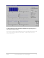
1
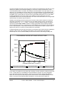
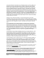
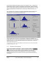
Software for estimating potential yield
under uncertainty
Final Technical Report
March 2001
Final Report - Administrative Details
DATE COMPLETED: Day\Month\Year:
30/1/2001
TITLE OF PROJECT
R 7041: Software for estimating potential yield
under uncertainty
PROGRAMME MANAGER / INSTITUTION
Professor John Beddington
MRAG Ltd
47 Princes Gate,
London SW7 2QA
FROM
1/ 01/96
REPORTING PERIOD
AUTHORS OF THIS REPORT
MRAG
TO
31/3/00
Dr G. P. Kirkwood
R 7041 Yield software – Final Technical Report
i
Acknowledgements
This project was funded through the UK Department for International Development (DfID)
Fisheries Management Science Programme (FMSP), which is managed by MRAG Ltd. The
project leader (Dr G Kirkwood) gratefully acknowledges the help of Trevor Branch in
specifying the software and the programming skills of Trevor Branch, Simon Nicholson and
Steve Zara during the writing and testing phases.
MRAG
R 7041 Yield software – Final Technical Report
ii
Table of Contents
Final Report - Administrative Details ................................................................i
Acknowledgements .......................................................................................... ii
Table of Contents............................................................................................ iii
Final Technical Report .................................................................................... 1
1. Executive Summary ............................................................................... 1
2. Background ............................................................................................ 1
3. Project Purpose...................................................................................... 4
4. Research Activities................................................................................. 4
5. Outputs................................................................................................... 5
5.1 Example analysis ............................................................................. 5
5.1.1 Parameters for L. mahensa. ....................................................... 5
5.1.2 Yield-per-recruit analyses........................................................... 9
5.1.3 Equilibrium yield analyses ........................................................ 12
5.1.4 Transient analyses ................................................................... 17
5.1.5 Summary .................................................................................. 19
6. Contribution of outputs ......................................................................... 20
7. References........................................................................................... 20
MRAG
R 7041 Yield software – Final Technical Report
iii
Final Technical Report
1.
Executive Summary
The FAO guidelines on the precautionary approach to management of capture fisheries and
the texts of several new international fishery management agreements indicate the
importance of precautionary reference points in the framing of fishery management advice.
The guidelines also emphasise the need to take proper account of uncertainty in this advice.
Following this advice poses a serious problem for fishery officers and scientists in developing
countries, since the calculations involved require a greater degree of analytical and
programming sophistication than is often available, and existing software packages commonly
used by them do not allow for such calculations. The Yield software package developed
during this project was aimed to fill this gap.
Written in Visual Basic, the software has a standard Windows user interface and a very
extensive on-line help system. It also incorporates a comprehensive example analysis of
data from an Indian Ocean snapper fishery. Users are able to specify levels of uncertainty in
each of the input parameters in terms of three possible probability distributions, and they can
also specify the level of inter-annual variability in annual recruitment. For each of the
calculations available in the software, results are presented in terms of frequency distributions
for the quantity concerned, rather than a single value as is usual, thus allowing the full extent
of uncertainty to be determined. Stochastic forward projections also taking account of
parameter uncertainty allow the user to explore further the likely result of different
management options.
The improved scientific advice will considerably enhance the likelihood of sustainable
management of vital fishery resources, which in developing countries often represent major
sources of animal protein, employment and income.
2. Background
For many years, the explicit or implicit primary management goal for most commercially
exploited fisheries was to take the maximum sustainable yield (MSY). One of the advantages
of this was that, provided time series of annual catches and catches per unit effort (CPUE)
were available, estimates of this quantity could be calculated by fitting simple stock production
models. With software packages such as CEDA (MRAG, 1992a), obtaining such estimates
and corresponding indications of the uncertainties associated with those estimates was within
the reach of fishery officers in developing countries.
In many fisheries, it is also possible to obtain estimates of von Bertalanffy growth curves (e.g.
using the LFDA software, MRAG 1992b). Provided an estimate is also available for the
natural mortality rate, then simple yield-per-recruit calculations can also be carried out, using
the software package FISAT (1997), for example. This then enables estimation of curves
relating the yield-per-recruit to the fishing mortality rate, F, and from that calculation of the
fishing mortality rate that produces the maximum yield-per-recruit (FMSY). In the absence of
estimates of the MSY, FMSY has at times been used as a target fishing mortality rate, but as
this often very large (indeed it is often infinite) and alternative target, F0.1, introduced by Dr
John Gulland, is often used in its place.
F0.1 is defined as the value of F such that the slope of the yield-per-recruit curve is 0.1 times
the slope of that curve at the origin. This apparently arbitrary definition always produces a
value of F that is less that the F at maximum yield-per-recruit FMaxYPR, and it is commonly of a
similar size to FMSY. It is, however, significantly harder to calculate.
MRAG
R 7041 Yield software – Final Technical Report
1
The final calculation that was commonly done is earlier stock assessments was that of curves
relating the spawning stock biomass (SSB) per recruit to the fishing mortality rate. These
curves illustrate that as F increases, the SSB-per-recruit decreases. For high values of F (e.g.
often for FMSY), the SSB-per-recruit is often only a very small fraction of its unexploited level.
Assuming that the numbers of recruits remain (on average) constant regardless of the size of
the SSB is a non-conservative one at best, but it is particularly dangerous for very low SSBs.
Following Beddington and Cooke (1983), if the SSB-per-recruit is less than 20% of its
unexploited level, it has commonly been taken as a rule of thumb that there is a non-ignorable
risk that future recruitment may be reduced.
Adopting a terminology that has now become common, these various values of F that have
often been calculated in stock assessments can be called reference points. The first three
mentioned above, (FMSY, FmaxYPR and F0.1) are known as target reference points, in that they
represent potential target values to aim for in setting appropriate levels of fishing mortality.
The last reference point, the F that produces a 20% SSB-per-recruit relative to its unexploited
level, is rather different. It has come to be known as a limit reference point, in that it is not a
target at all; rather it is a level of F that should not be exceeded.
A typical illustration of these reference points is in the figure below, which plots the equilibrium
yield per 1000 recruits, the equilibrium yield (taking a non-constant stock recruitment
relationship into account) and the SSB-per-recruit as functions of the fishing mortality rate.
EQUILIBRIUM YIELDS WITH AND WITHOUT SRR
90.0
80.0
20000.0
YIELD
70.0
60.0
15000.0
50.0
10000.0
40.0
30.0
20.0
5000.0
10.0
0.0
0.00
0.20
0.40
0.60
0.80
SSB-per-recruit (% unexploited)
100.0
25000.0
0.0
1.00
FISHING MORTALITY RATE F
YIELD PER 1000 RECTS
YIELD WITH SRR
F0.1
SSB-per-recruit
In this figure, the yield-per-recruit rises with increasing F until it reaches a maximum at around
F=0.8. At this value of F, the SSB-per-recruit has fallen to around 10% of its unexploited
level, well below the 20% rule of thumb. When a stock-recruitment relationship (SRR) is
taken into account (but one that still produces 1000 recruits in its unexploited state), we see
that the recruitment has definitely fallen well before F reaches this level; indeed the
MRAG
R 7041 Yield software – Final Technical Report
2
equilibrium yield is now only at 25% of its real maximum (at F=0.2). In contrast, for the
parameters used to calculate this figure, the value of F0.1 is 0.26, only marginally above the
true FMSY, with a corresponding SSB-per-recruit of around 35% of its unexploited level.
One final point to note about the calculation of reference points described above is that they
assume the population is in deterministic equilibrium. In particular, this means that they
assume that there is no stochastic variability in annual recruitment. Perhaps the one thing
that is common to fish stocks is that all appear to demonstrate considerable interannual
variability in recruitment; see for example Myers et al (1995). This is an issue also addressed
by Beddington and Cooke (1983), who found, in particular, that stochastic variation in
recruitment can, with high probability, reduce the SSB below a fixed level even though
deterministic calculations show that the equilibrium SSB will be above that value.
By the early 1990s, particularly following the UNCED Rio declaration, it had become clear that
to avoid yet more stocks moving into the overexploited category, it was necessary to adopt a
more precautionary approach to fishery management. One outcome of this realisation was a
set of guidelines for a precautionary approach to capture fisheries (FAO, 1995) that
emphasised, inter alia, of calculating and using both target and limit reference points, and of
taking full account of uncertainties and associated risks. The FAO Code of Conduct for
Responsible Fisheries, which soon followed the publication of the guidelines, also
incorporated these sentiments.
Perhaps the most recent and most clearly expressed exposition of these ideas is contained in
Annex II to the Draft Agreement for the Implementation of the Provisions of the United
Nations Convention on the Law of the Sea of 10 December 1982 Relating to the Conservation
and Management of Straddling Fish Stocks and Highly Migratory Fish Stocks. This is
reproduced below.
GUIDELINES FOR APPLICATION OF PRECAUTIONARY REFERENCE
POINTS IN CONSERVATION AND MANAGEMENT OF STRADDLING FISH
STOCKS AND HIGHLY MIGRATORY FISH STOCKS.
1. A precautionary reference point is an estimated value derived through an
agreed scientific procedure, which corresponds to the state of the resource
and of the fishery, and which can be used as a guide for fisheries
management
2. Two types of precautionary reference points should be used: conservation,
or limit, reference points and management, or target, reference points. Limit
reference points set boundaries which are intended to constrain harvesting
within safe biological limits within which the stocks can produce maximum
sustainable yield. Target reference points are intended to meet management
objectives.
3. Precautionary reference points should be stock-specific to account, inter
alia, for the reproductive capacity, the resilience of each stock and the
characteristics of fisheries exploiting the stock, as well as other sources of
mortality and major sources of uncertainty.
4. Management strategies shall seek to maintain or restore populations of
harvested stocks, and where necessary associated or dependent species, at
levels consistent with previously agreed precautionary reference points. Such
reference points shall be used to trigger pre-agreed conservation and
management action. Management strategies shall include measures which
can be implemented when
precautionary reference points are approached.
5. Fishery management strategies shall ensure that the risk of exceeding
limit reference points is very low. If a stock falls below a limit reference point
MRAG
R 7041 Yield software – Final Technical Report
3
or is at risk of falling below such a reference point, conservation and
management action should be initiated to facilitate stock recovery. Fishery
management strategies shall ensure that target reference points are not
exceeded on average.
6. When information for determining reference points for a fishery is poor or
absent, provisional reference points shall be set. Provisional reference points
may be established by analogy to similar and better-known stocks. In such
situations, the fishery shall be subject to enhanced monitoring so as to
enable revision of provisional reference points as improved information
becomes available.
7. The fishing mortality rate which generates maximum sustainable yield
should be regarded as a minimum standard for limit reference points. For
stocks which are not over-fished, fishery management strategies shall ensure
that fishing mortality does not exceed that which corresponds to maximum
sustainable yield, and that the biomass does not fall below a pre-defined
threshold. For over-fished stocks, the biomass which would produce
maximum sustainable yield can serve as a rebuilding target.
These requirements are all exemplary and the calculation of the various quantities involved is
well within the scope of large fisheries departments in developed countries. But such
calculations represent a really daunting task for many developing country fisheries officers.
The aim of the Yield software package developed under this project is to allow them to make
these calculations with ease, even in circumstances where knowledge of some of the
biological parameters required is poor and there may be strong stochastic variability in
recruitment.
3. Project Purpose
To develop and disseminate a user-friendly, windows-based, software package for estimating
potential yields, which properly takes into account uncertainty in biological parameter
estimates and inter-annual variability in recruitment. Users will be able to estimate yields that
are compatible with differing management objectives. Comprehensive tutorials and manuals
will accompany the software.
4. Research Activities
The research activities consisted of specifying the software, programming it in object-oriented
Visual Basic, testing, incorporation of a comprehensive on-line help system and including a
detailed expository example analysis of data for an Indian Ocean snapper and emperor
fishery. The final version was sent to two expert external reviewers, and then revised in light
of their comments. The software will be disseminated through the new FMSP web site.
MRAG
R 7041 Yield software – Final Technical Report
4
5. Outputs
5.1 Example analysis
We present here an example analysis of yields and yield reference points using data for
Lethrinus mahensa, one of the main species taken in fisheries for snappers and emperors in
the western central Indian Ocean, on banks around the Chagos Archipelago, the Seychelles,
and Mauritius.
The aim is to illustrate how to collate and enter appropriate information on the biological and
fishery parameters and their uncertainties, and how to interpret the results from the various
analyses carried out using the software. In order to avoid duplication and to keep this
example analysis down to a reasonable length, we omit details on the mechanics of using the
software. Instead, links are given at appropriate places to relevant sections of the Help files,
where comprehensive information on these aspects may be found.
For users unfamiliar with the types of analyses carried out in this software package, we
suggest that you first simply read through the example analysis, diverting to appropriate
sections of the help files for more information as needed. Having done so, we then suggest
that you attempt to repeat the analyses, as suggested in the text. Before doing so, however,
we strongly suggest that you print out this section of the help files, as you will find that
switching back and forth between analysis and the help files is tedious at best.
5.1.1
Parameters for L. mahensa.
A data file containing estimates of parameters and their uncertainties for L. mahensa,
LmahDat.txt, has been distributed along with the software. After starting the Yield software,
load this parameter file (see Load parameters). The name of the species and the data file
should then appear in the header of the main form.
Biological and fishery parameters contained in the loaded data file may be inspected (and
changed or entered; see Entering parameters) using the Parameters menu. The first item on
that menu is Von Bertalanffy… , which allows the von Bertalanffy growth parameters and
their uncertainties specified in the parameter file to be inspected (see Entering von Bertalanffy
parameters). Selecting this menu item will reveal that uncertainties have been specified for
L∞ and K, but not for t0. Delving further, you will find (see Choose distribution for uncertainty in
Linfinity) that L∞ has been specified to have a normal distribution with mean = 53.6 and CV =
0.08; K has a lognormal distribution with mean = 0.128 and CV = 0.17; and t0 has a value
fixed at 0.
Where did these values come from? The best potential source of information for these and all
the other parameters obviously is data collected directly for the species and from the fishery
itself. This is the source used for the L. mahensa parameters. For the growth parameters,
both length frequency distributions and age-length data were collected for each of the main
fisheries in the western central Indian Ocean during a UK Department for International
Development (DFID) funded project carried out by MRAG Ltd. The results were described in
Pilling et al (1999) and in a PhD thesis by Dr G. Pilling (1999). For L. mahensa, the length
frequency data were analysed using the Elefan method as implemented in the LFDA software
(MRAG, 1992), and estimates of von Bertalanffy parameters were obtained by non-linear
regression analysis of the age-length data. The means and CVs quoted are the means and
CVs of the sets of estimates obtained (there were 12 in all).
As for the distributions, there is an element of arbitrariness in their selection. With just 12
individual estimates, it is rather difficult to identify an appropriate distribution with any degree
of certainty. The distribution of estimates of L∞ was roughly symmetrical; hence the choice of
the normal distribution. The distribution of estimates of K was also reasonably symmetrical,
but there was a hint of a slightly longer tail towards higher values of K. More importantly,
however, it is known that K must be greater than zero. Negative values can be avoided by
MRAG
R 7041 Yield software – Final Technical Report
5
using a lognormal distribution, which in any case can also be reasonably close to
symmetrical; see the plot of the selected distribution for K.
Users with experience in estimating growth parameters may be rather suspicious of the
relatively low levels of variability in L∞ and K, and even more so of the apparently certain and
suspiciously round value of t0. They have every right to be. It is usually impossible when
analysing the types of length frequency data available using the Elefan method to obtain any
estimates of t0. However, such is not the case when estimating growth parameters using
age-length data. In practice, the age-length data available contained very few observations
for small ages and lengths. The implication of this is that it is actually very difficult to estimate
all three von Bertalanffy parameters with any precision at all: the data were compatible with
quite large negative values of t0 (which went with low K and high L∞ values) or small values of
t0 (which went with high K and low L∞ values). The estimates used here in the end were
those corresponding to t0 = 0. Taking this approach almost certainly underestimates the true
uncertainties in growth parameters, but it suffices for this example.
A final, rather technical point should also be made here. Even ignoring the parameter t0, it is
almost universally observed that when estimates of L∞ and K are being calculated, either
using individual data sets or combining sets of estimates from different data sets, there tends
to be a high negative correlation between the two. In the L. mahensa case, the correlation is
as high as –0.89. When originally specifying the software, we were well aware of this issue,
but given the almost complete lack of cited estimates of the correlation between L∞ and K in
the literature, we decided to ignore it. In retrospect, this may not have been the right decision,
and later versions of the software will allow the user at least to enter a value for the
correlation between L∞ and K. The current version assumes that the two parameters are
independent. (Note that in Dr Pilling’s final analyses, account was taken both of individual
variability in growth parameters and of estimated correlations between all three growth
parameters, but this requires methods far beyond the scope of this software package).
How might users collate the information needed to specify means and CVs for von Bertalanffy
parameters? If they are lucky, data will be available (or can be collected) from their fishery to
allow direct estimation of mean values at least. Note, however, that no reliable estimates of
growth parameter uncertainty are available from any currently-used method for analysing
length frequency data, so there still remains a problem there. Fortunately, even if no direct
estimates are available for your species and fishery, the excellent and comprehensive
database FishBase 98 almost certainly will have recorded estimates of biological parameters
for the species concerned or a closely related species. This should allow at least a rough
idea to be gained as to appropriate mean values and likely ranges of values of the von
Bertalanffy growth parameters. Be warned, however, that some judgement still needs to be
used when using data from related species. For example, even if attention is restricted to
lethrinid species, recorded pairs of estimates of L∞ and K range from (16.2, 0.86) for L.
genivittatus in New Caledonia to (106, 0.061) for L. olivaceus in the Yemen. Given the L.
mahensa data, neither are at all likely for this species.
Turing to length-weight parameters (see Entering Length-weight parameters), you will see
that only single values have been entered in the L. mahensa data set. Length-weight data
are perhaps the easiest biological data of all to collect and analyse, and in most cases they
show relatively low levels of variability. That was certainly the case with the L. mahensa data,
and we have opted not to specify uncertainties around the entered values.
If length-weight parameters are the easiest to estimate, the next parameter, the natural
mortality rate, is almost certainly close to the hardest. Fortunately, the empirical relationship
developed by Pauly (1980) and FishBase 98 come to our rescue again. Two options are
available after selecting the Natural mortality… item from the Parameters menu: the user
can enter a single value (or distribution) for the natural mortality rate, or use Pauly’s (1980)
empirical relationship (see Enter natural mortality rate, Enter parameters for Pauly’s
equation). For L. mahensa, we also had no reliable direct estimate of the natural mortality
rate available, so for this example we have opted to use Pauly’s relationship. The temperature
entered (27°C) was extracted from the Nautical Almanac for the Indian Ocean. No
uncertainty has been specified about this temperature.
MRAG
R 7041 Yield software – Final Technical Report
6
While estimates of the natural mortality rate are available from FishBase 98 for at least some
species, many of these have been calculated using Pauly’s equation. Unless you have
available an estimate or estimates of the natural mortality rate that you consider to be quite
reliable, we would suggest in most cases that you use the Pauly’s equation option, and
certainly that you use this option rather than enter a single value that itself was calculated
using this relationship. The reason is that, if you use the Enter parameters for Pauly’s
equation option directly, then the uncertainties you entered for the von Bertalanffy
parameters will automatically be taken into account in the simulations, and they will by
themselves induce uncertainties in the value of the natural mortality rate.
The next parameters to be entered are the maturity and capture parameters (see Maturity and
Capture). For L. mahensa, we have opted to enter lengths, rather than ages, and we
anticipate that this choice will be made most times when the software is used (if for no other
reason that ages are often so hard to estimate directly). Based on data collected from the
fisheries, the (knife-edge) length at maturity has been set to have a lognormal distribution with
mean = 27.6 cm and CV = 0.05. The mean and CV were estimated from data on the lengths
at which 50% of the fish first attained maturity, and the lognormal distribution was used
because the ogive of proportions mature at length was rather steeper at low lengths than at
higher lengths, suggesting that the distribution of length at 50% maturity had a slightly longer
tail towards higher lengths.
The length at first capture was set at a constant value of 22.8 cm. This, of course, is one of
the parameters that can, in principle, be changed by management regulation (e.g. by setting
minimum landing sizes, or mesh sizes). The actual mean lengths at first capture differ
amongst the different fisheries in the western central Indian Ocean, however here seems little
point in reflecting this in the uncertainties in this parameter. However, if the mean length at
first capture tended to differ substantially between years in an individual fishery, then it would
be entirely appropriate to specify uncertainties about this parameter.
The next items to specify are the seasons (see Spawning and Fishing seasons). Three things
need to be set. The first is the time step interval. Here, we have set this as Monthly. This is
not strictly necessary in order to specify the spawning and fishing seasons, which have been
taken to occur all year round based on available information. However, using a yearly time
step is likely to lead to inaccuracies in the numerical calculations for a species that only lives
for a maximum of 15 – 20 years, so Months is the appropriate time step.
The last set of parameters to enter are those for the stock-recruitment relationship (see
Choose type of stock recruit relationship). This is even harder that setting the natural
mortality rate, and at least one of the values entered here is, to be honest, partly a guess. It
may seem rather odd to admit this in what is a demonstration of the use of the software, but in
many cases, it is likely that this will also be the situation facing the typical user, especially
those in developing countries with relatively little information available about their fishery. It
therefore seems appropriate to attempt to demonstrate what can be done in such cases.
The first choice to be made is of the form of stock-recruit relationship. That is relatively easy.
The only two real possibilities in the current context are Beverton and Holt, or Ricker. The
Ricker relationship, most commonly seen in the context of salmon stocks, is generally thought
to apply in circumstances where there is either very substantial cannibalism or where there
are restricted spawning areas. Neither is thought to apply to L. mahensa, so a Beverton and
Holt relationship seems the most appropriate, as it is likely to be in most cases. With regard
to the parameters (see Beverton and Holt SRR- Standard formulation, Beverton and Holt
SRR- Steepness formulation), whichever is chosen, there are essentially two to specify.
One of these is the so-called steepness parameter. There is some external information
available on typical values of this parameter. This comes from the data originally collated by
Myers et al (1995), now included in FishBase 98. Based on values included in this database
for related species, Mees and Rousseau (1997) identified a lower limit for a related parameter
that was equivalent to a steepness parameter of 0.8. On those grounds, we have chosen to
assume that the steepness parameter is uniformly distributed between 0.8 and 0.95.
MRAG
R 7041 Yield software – Final Technical Report
7
The second parameter is the maximum (or unexploited) number of recruits (or SSB). This
parameter is, of course, entirely stock-specific. Small stocks will have a small maximum
number of recruits; large stocks will have a large number. What that number is will be a
function of the fecundity of the stock, the productivity of the waters in which it spawns, the
size of the available spawning or nursery areas, and so on. Regrettably, such information
cannot be gleaned from estimates obtained from related species, or the same species in
different areas. If you are very fortunate, then an abundance survey may have been carried
out prior to or shortly after the fishery was discovered. This may well provide estimates of the
unexploited number of recruits or of the adult biomass. If so, then it is a relatively trivial
matter to enter an appropriate value (with uncertainties) once the Use estimates of biomass
or recruits option is selected. Alternatively, in other cases, estimates are sometimes
available of biomass per unit area (perhaps between certain depth ranges in which the stock
is found). Again, such information can in principle readily be used in conjunction with widelyavailable bathymetric information.
Failing this, there is little else to fall back on, and an educated guess must be made.
Fortunately, at least in terms of the reference points for the fishing mortality rate, this matters
much less than might be imagined, as will be seen later. One possible approach is to choose
a value for the unexploited number of recruits that produces a maximum sustainable yield that
is of the same order of magnitude as catches, or preferably, other estimates of potential
yields.
For the shallow banks of the Chagos Archipelago, the potential yield for commercially
important handline species may be approximated by comparison with yields observed in
similar areas in the Indian Ocean. For example, Sanders (1988) assumed that the potential
yield of the Chagos Bank would be equivalent to that observed on the more heavily exploited
-2
Saya de Malha bank north of Mauritius (0.22 t km ). In the Seychelles, the sustainable yield
-2
in shallow water strata was estimated to be 0.168 t km (Mees, 1992). However, catch rates
in the Chagos Archipelago are less than in Seychelles or on the Saya de Malha bank. Thus, a
-2
more conservative estimate of 0.100 t km may be more appropriate for the Chagos
Archipelago.
2
The estimated area of the Chagos Archipelago less than 70m in depth is 8587 km . Using
the above figures, estimates of the sustainable annual yield for the shallow sector of the
Chagos Archipelago range from around 860 to 1,900 t (Mees et al., 1999). Using the mean
values only for all other input parameters, some simple experimentation suggests that an
unexploited number of recruits of 25 millions produces a mean MSY of 1430 t, which is
roughly in the middle of this range. This value was therefore used for R0, but no uncertainty
was allowed, to reflect the somewhat arbitrary nature of the value.
The final parameter to enter on this form is the CV of inter-annual recruitment variability. In
many cases, this will also be an elusive parameter. For L. mahensa, age frequency data
were available for a number of years, and it was therefore possible, using an assumed
constant value for M, to project backwards and estimate numbers at age 0 in a number of
years. The CV of these estimates was 0.25. Should such data not be available (as it most
likely will not be for your fishery), then it should be possible to select at least a plausible value
using the Meyers et al (1995) and FishBase 98 data. It may be sensible to try different
analyses with different CVs (see later).
The last information to enter serves essentially as documentation of the analysis: the fishery
description (see Fishery description). For the example data file, you will see the species
name and a brief description of the fisheries.
Now that everything has been entered, it is time to see if they are all compatible and within
sensible ranges. This is achieved using the Cross-check parameters menu item (see
Cross-check parameters). Selecting this item, you should find that all parameters are
consistent. So they should be, given that we set up the example parameter file! It is,
however, worth following through the example in the help file for this menu item, in which the
value of the natural mortality rate is deliberately changed to something silly, just to gain
MRAG
R 7041 Yield software – Final Technical Report
8
practice in seeing what to do if the parameters are found not to be consistent. But if you do
so, don’t forget to change the natural mortality rate back to what it was originally before
proceeding.
If you had been entering a new data set, it would now be worthwhile saving the parameters
(see Save parameters), though this is not necessary in this case.
5.1.2
Yield-per-recruit analyses
The first analysis to carry out is of the equilibrium yield-per-recruit (see Equilibrium yield-perrecruit and related help files). Select Yield-per-recruit v F… from the Equilibrium menu.
Accept the range of values of F over which the calculations will be performed (click OK). After
a while, a series of plots will appear. Those illustrated below are displayed as fractions of
unexploited biomass (see Calculate equilibrium yields and biomasses per recruit). This is
frequently the most useful display option, as absolute values are not really important.
Note that when you do these calculations, the results will not be identical to those illustrated in
this example analysis. This is because you will have used different sets of random numbers
(see Random seed). They should, however, not be too different!
The top-left plot shows that the median yield-per-recruit, as a fraction of unexploited fishable
biomass, reaches a maximum or close to one at values of F above about 1.3. Recall the
mean value of M was around 0.39, so the F producing the median maximum yield per recruit
is at least 3 times M, which is quite a high value. The upper 97.5% confidence band for
relative yield-per-recruit is still rising as F reaches 2.0, while the lower 2.5% confidence band
may have reached a maximum for F somewhere over 1.1. Yield-per-recruit plots that suggest
the maximum occurs at high values of F are very common. Whether or not this occurs is
largely determined by the relative values of M and K, and even more so by the relative values
of the length at first capture and length at maturity. This should not be taken to suggest that
the stock can withstand almost any level of fishing mortality, as the remaining plots show.
The other plots show the relationship between various biomasses-per-recruit, as a fraction of
their unexploited level, and F. Here, we shall only comment on the relative SSB-per-recruit.
Whether one looks at the median, or at either confidence band, it is clear that levels of F that
MRAG
R 7041 Yield software – Final Technical Report
9
produce yields-per-recruit at or near the maximum will also reduce the SSB to levels that are
a tiny fraction of its unexploited level. Remember that yield-per-recruit analyses explicitly
assume that recruitment is unaffected regardless of how low the SSB falls. This is extremely
unlikely when the SSB is reduced to levels seen in the plot for high values of F.
Before moving on, if you wish to keep a record of your analyses, you may wish to print out a
copy of this form. Also, if you want to see the results in more detail, you can do so clicking
the Medians and intervals button.
The next step in the analysis is to calculate yield and biomass per recruit reference points
(see What are reference points?, Calculate equilibrium yield-per-recruit reference points).
Select Yield-per-recruit reference points… from the Equilibrium menu. You will see three
reference points have been checked for calculation (Maximum yield-per-recruit, F0.1 and the
target SSB/Initial = 0.2). Click OK to accept these and in time a results form similar to the one
below will appear. The first to be illustrated is that for maximum yield-per-recruit. Again, the
display option chosen is as a fraction of unexploited biomass. For more details, see
Equilibrium yield-per-recruit reference points: Interpreting the results.
This form displays 6 histograms. The top left one is of the fishing mortality rate that produces
the maximum yield-per-recruit. The way in which these results are calculated is explained in
detail in the Simulating under uncertainty section of the Help files. For the purposes of
explanation here, we simply note that 100 simulations were carried out (you can check this by
selecting Number of simulations in the Options menu, but don’t do so right now, as the
results form will then disappear and it will have to be produced again). The numbers
appearing on the x-axis of the histogram correspond to the mid-points of each histogram bin.
Thus the first bin, labelled 0.9, in this case refers to values of F in the range 0.6 – 1.6, the
second to 1.6 – 2.6, and so on.
The largest frequency (for F in the range 1.6 – 2.6) has around 30 observations. Note the
occurrence of 28 cases of “infinite”F. Quotes are used here because any F greater than
around 20 times the mean value of M used (0.392) is treated as being effectively infinite.
MRAG
R 7041 Yield software – Final Technical Report
10
Over 50% of the time, the F producing the maximum yield-per-recruit exceeded 2.4. This
confirms the impression given by the yield-per-recruit plots discussed above.
The SSB-per-recruit histogram also confirms the impression given by the earlier plots: the
largest of all the values of SSB-per-recruit was less than 11% of its unexploited value. Note
that, while the first bin (labelled 0) of this histogram nominally refers to values in the range –
0.0065 to 0.0065, since negative values of SSB-per-recruit are impossible, it actually refers to
the range 0 to 0.0065. Defining algorithms for automatic labelling of histograms is difficult,
and we have not always got it absolutely right. This is why the user is offered the option of
producing a table of results, which can be transferred to your favourite graphics package to
produce final publication-quality plots.
Clearly, the maximum yield-per-recruit reference point is not one that can safely be used as a
management target for this species.
The next reference point to examine is the F0.1 reference point. Selecting results for F0.1
produces the following form (again using the Fraction of unexploited biomass display
option).
As explained in the What are F0.x reference points? Help item, the F0.1 yield-per-recruit
reference point has a rather odd definition, but it has proved rather useful in practice,
especially in circumstances, such as the ones seen here, when the maximum-yield-per-recruit
reference point is obviously not particularly useful.
The most frequently occurring value of F0.1 lies in the range 0.37 – 0.39, and the maximum in
the range 0.57 – 0.61. Compared with the mean M (0.392), these are obviously more
sensible values of F. Also, in the majority of cases, the SSB-per-recruit corresponding to F0.1
exceeds 20% of its unexploited level, a proportion often treated as one below which one
would prefer not to fall.
MRAG
R 7041 Yield software – Final Technical Report
11
We will need the median and confidence limits for the estimated F0.1 later. Clicking on the
Results button will produce a table of the results of all 100 simulations. Select and copy the
Fishing mortality column, paste it into a spreadsheet, and then sort the column in ascending
order. It is then simple to estimate the median and lower and upper 2.5%iles of F0.1. For the
example illustrated above, the median was 0.40, with a 95% confidence interval of 0.31 –
0.54.
This comparison can be revisited by examining the third reference point calculated, which
determines values of F the produce an equilibrium SSB-per-recruit that is 20% of its
unexploited level. Typical results are illustrated below.
The most obvious result in this form is in the histogram for SSB-per-recruit/SSB0. As it
should, it shows that in every case, this ratio was 20%. Looking at the histogram of values of
F that produce this, we see that most frequently, these fell in the range 0.37 – 0.43, and all fell
between 0.25 and 0.79. As one would have expected, these reference point F values are
slightly higher than those for F0.1.
Using the table of results, the median SSB-per-recruit reference point F was 0.45 with 95%
confidence interval 0.31 – 0.70.
5.1.3
Equilibrium yield analyses
We turn now to equilibrium yield analyses. These are described in detail in the Equilibrium
yield and related sections of the help files. Equilibrium yield analyses allow the user not to
have to assume that recruitment remains constant regardless of how low the SSB falls, but
this gain is achieved only at the expense of having to specify the stock-recruitment
relationship, which we have seen can be difficult at best. In this section, we attempt to
illustrate the analyses that can be carried out, and how to get around these difficulties (at
least partially).
MRAG
R 7041 Yield software – Final Technical Report
12
Select Equilibrium yield from the Equilibrium menu and accept the range of F values
shown. After a while, the following form appears, after the Fraction of unexploited biomass
display option has been selected.
Comparing these plots with the corresponding ones for yield-per-recruit demonstrates starkly
what a difference it can make when account is take of recruitment falling with falling SSB.
The plot of relative yield against F suggests that in 97.5% of the simulations, the stock was
nearly extinguished when F reached a level of 2. For the median, the maximum yield
occurred at an F around 0.4, and for the lower 2.5%ile, F had to lie in the range 0 – 0.8 to
produce any sustainable yield at all. The other plots show a similar story. In particular, to
achieve a median SSB/SSB0 ratio of 20%, the corresponding F value seems to be around
0.4.
One other interesting point to note is the shape of the plot of yield against F. The standard
Schaeffer biomass dynamic model suggests that the yield curve is symmetric. This curve is
clearly asymmetric, with a peak shifted towards lower values of F.
If you had been able to use a direct estimate of the unexploited number of recruits or SSB
when entering the parameters of the stock-recruitment relationship, then the other display
option (Absolute biomass) becomes much more relevant. While this is not the case here,
on selecting that display mode (try it and see), you should find that the median maximum yield
(MSY) is around 1400 tonnes, but the MSY could lie between approximately 750 and 2750
tonnes. This is a fairly high level of uncertainty if you were wishing to set annual quota based
on the estimated MSY! Remember that, because you will be using different random numbers,
the actual values you get will differ from those quoted here.
Let us turn now to the equilibrium yield reference points (see Equilibrium yield reference
points and related help files for more details). Select Equilibrium yield reference points
from the Equilibrium menu and accept the options checked, noting that an additional
reference point has been asked for: that producing a fishable biomass at 50% of its
unexploited level. This has been added to the example at this stage because the much-used
MRAG
R 7041 Yield software – Final Technical Report
13
Schaeffer biomass dynamic model suggests that the MSY can be taken when the fishable
stock has been reduced to 50% of its unexploited level.
The most frequently occurring values of FMSY lie in the range 0.39 – 0.45, with a range
extending from 0.21 to 0.75. Using the table of results, we find that the median value of FMSY
is 0.41 with 95% confidence limits of 0.27 to 0.70. Looking at the histogram of values of
SSB/SSB0, we see that in the clear majority of cases, these are less than 20% when the
stock is being fished at FMSY.
This latter observation, of course, can be interpreted in two ways. On the one hand, given the
concern often expressed about reduction of the SSB to levels below 20% of its unexploited
level, it might be suggested that even fishing at a mortality rate that produces the MSY may
be rather less safe than might have been imagined. On the other hand, it could equally be
argued that, for this species and fishery, associating dangers of stock collapse with a 20%
SSB/SSB0 level is being rather too conservative. Reaching a considered view on this must
be delayed until we have seen the results of calculating the transient SSB reference point,
when recruitment variability is also taken into account. However, for the moment it is worth
recalling that we have assumed that the steepness parameter of the Beverton and Holt stockrecruitment relationship lies between 0.8 and 0.95. By definition, this means that when the
SSB has been reduced to 20% of its unexploited level, the recruitment lies between 80% and
95% of its equilibrium unexploited level.
The last point to note from these histograms is that, most frequently, the maximum yield
occurs when the fishable biomass is around 30% of its unexploited: quite a long way below
the 50% suggested by the Schaeffer model.
Reverting to an absolute biomass display option confirms our earlier views as to the likely
MSY levels. The catch histogram indicates that the most frequently occurring MSYs lie in the
range 1500 – 1700 tonnes, but the MSY could be as low as 400 tonnes and as high as 2800
tonnes. Remember, however, that these absolute biomass plots must be taken with a large
grain of salt, because we were forced to use a somewhat arbitrary value for the unexploited
number of recruits. We will return to this point a little later.
MRAG
R 7041 Yield software – Final Technical Report
14
Now look at the target spawning biomass reference point. Histograms displayed as fractions
of unexploited biomass are illustrated below. Recall that the target is 20% SSB/SSB0.
Recall that earlier we noted that when fishing at FMSY, in the majority of cases the SSB/SSB0
ratio was less than 20%. That implies, of course, that if we shift our target to a 20% SB/SSB0
ratio, the reference point Fs to achieve that should be less than those to achieve MSY. The
above histograms clearly support this. Now, the mode occurs between 0.355 and 0.405, and
using the table of results, the median was estimated to be 0.37, with 95% confidence interval
0.25 – 0.54.
Finally, look at the 50% target fishable biomass reference point. Again, we would expect this
to be achieved at a considerable lower value of F, given the median fishable biomass ratio
producing MSY was estimated earlier to be 30%. The histograms below clearly support that
contention. Now, the mode occurs at an F around 0.211. Using the table of results, the
median was estimated to be 0.20, with 95% confidence interval 0.15 – 0.26.
MRAG
R 7041 Yield software – Final Technical Report
15
All these results seem consistent (they should be as long as the calculations have been
performed correctly!). But recall that one of the stock-recruitment parameters was somewhat
arbitrarily selected (the unexploited number of recruits, R0 = 25 million). We asserted earlier
that this may not be as big an obstacle to getting reliable results as may be expected.
To see this whether or not this is so, let us go back and alter the value for the unexploited
number of recruits by a factor of 10 either way. Via the Parameters | Stock-recruit
relationship menu item, alter R0 from 25 million first to 2.5 million and the recalculate the
MSY reference point. When we did this, we found that the median F that produces MSY was
0.43, with 95% confidence interval 0.31- 0.64. Naturally, the median MSY was much smaller
(around 152 tonnes, not coincidentally about 10 times smaller than when R0 was 25 million).
Now repeat the process, but now change R0 to 250 million, 10 times larger than it was. We
found that the median F that produces MSY was 0.42 (95% confidence interval 0.28 – 0.68),
but the MSY is now (again not coincidentally) about 10 times larger.
Recalling that the median value of FMSY when R0 was 25 million was 0.41, it appears that our
assertion was correct. At least in terms of estimating fishing mortality reference points, it
does not appear necessary that R0 is estimated with precision. However, in terms of
estimating the MSY itself, of course, it is clear that considerable precision is needed.
MRAG
R 7041 Yield software – Final Technical Report
16
5.1.4
Transient analyses
Finally we turn to the last set of analyses. These allow us to get away from the restrictive
assumption that the population is at equilibrium and to take account of interannual variability
in recruitment.
First we calculate the transient yield reference point (see Calculate the transient SSB
reference point and What is the transient SSB reference point?).
Note that this calculation will take considerable time when a monthly time step is used. If you
have a relatively slow computer, and have got rather bored waiting for the results to appear
on earlier calculations, we suggest you first change the time step interval (using the
Parameters | Seasons menu item) to Yearly.
Accept the targets that appear on the reference point form, including the target of 20%
SSB/SSB0. After some time, you should find that the fishing mortality rate that ensures that
only 10% of the time does the SSB fall below 20% of SSB0 in 20 years is around 0.26, which
is the value we obtained.
This value is rather less than the median FMSY (0.41), but then we would expect that because
that F on average reduces the SSB to less than 20% of its unexploited level even when there
is no recruitment variability. A fairer comparison would be with the median F that reduced the
equilibrium SSB to 20% of its unexploited level. That median F was 0.37, with a lower
2.5%ile of 0.25. The transient SSB reference point F is again well below the median; indeed
it is close to the lower 2.5%ile.
What this implies is that, with even relatively modest amounts of recruitment variability (and a
CV of 0.25 does merit being described as modest), the risks of the SSB falling below
specified low levels can be rather greater than might have been imagined.
The effects of recruitment variability on future projections can also be examined using the
Projections… item of the Transient menu (see Transient projections). Select this item and
try projecting forward for 20 years with an F of 0.26, and also starting with an equilibrium F of
0.26 (or whatever value you found for the transient SSB reference point).
You should find your results resemble those shown below, when the fraction of unexploited
biomass display option is selected.
MRAG
R 7041 Yield software – Final Technical Report
17
As expected, this shows that 95% of the time, the SSB/SSB0 rations lay between 0.2 and
around 0.45. Note that the median SSB/SSB0 ratio is around 0.32. Again, this gives an idea
of the effects of recruitment variability.
Given this, it is of interest to examine projections using the median FMSY reference point (0.41)
and the median equilibrium SSB reference point (0.37). Using the smaller value first, the
results are shown below.
MRAG
R 7041 Yield software – Final Technical Report
18
Now the median SSB/SSB0 ratio hovers just above 0.2, but the lower 2.5%iles lie around 0.1.
If you repeat this exercise with the median FMSY, you should find now that the median
SSB/SSB0 ratio now lies below 0.2, and the lower 2.5%ile is consistently around 0.09.
While there may well be arguments that a 20% SSB/SSB0 level is not particularly dangerous
for this species, a level less than 10% certainly is more dangerous: if the steepness
parameter really is a s low as 0.8, when the SSB is 9% of SSB0, the recruitment predicted
from the stock-recruitment relationship is only 62% of its unexploited level.
5.1.5
Summary
All that is left now is to collate the results and see what conclusions we can draw.
All the various reference points we have calculated are listed in the table below, excepting the
maximum yield-per-recruit reference point.
Reference Point
2.5 %ile
Median
97.5 %ile
F0.1
Equilibrium 20% SSB-per-recruit
FMSY
Equilibrium 20% SSB
Equilibrium 50% Fishable biomass
Transient 20% SSB
0.31
0.31
0.27
0.25
0.15
0.40
0.45
0.41
0.37
0.20
0.26
0.54
0.70
0.70
0.54
0.26
Looking first at the medians, we see that with the exception of the fishable biomass reference
point (which arguably can be discounted since the target level of 50% is probably rather too
high), all the median equilibrium reference points are similar and approximately equal to the
MRAG
R 7041 Yield software – Final Technical Report
19
mean value of M (0.39). This quite often is the case. The transient SSB reference point is,
however, rather lower; indeed it is lower than the lower 2.5%iles of the main equilibrium
reference point Fs. On the basis of these results, it would not be unreasonable to conclude
that a suitable precautionary target level for the fishing mortality rate might be in the range
0.25 – 0.35.
Parameter uncertainty has obviously played an important role in this analysis, given the rather
wide confidence limits for the reference point Fs. It also played a part in the calculation of the
transient SSB reference point. To see this, we deliberately removed all uncertainties in the
biological and fishery parameters (but retained the recruitment variability). With no parameter
uncertainty, the transient SSB reference point F was recalculated to be 0.31. As time passes,
one would expect that the extent of parameter uncertainty will be reduced, and thus
uncertainty in the equilibrium reference point Fs will reduce. However, the passage of time
will not affect recruitment variability. This analysis therefore suggests that even apparently
conservative equilibrium reference points may be rather less conservative than they appear,
when interannual recruitment variability is taken into account.
What does the analysis imply for the Chagos Archipelago fishery for L. mahensa? At present,
it is believed that this fishery is lightly exploited, with an F of the order of 0.2. The analysis
therefore suggests that an increase in F of up to 50% is likely to lead to increased sustainable
catches. If such an increase were allowed, however, it would be important that it be strictly
monitored.
6. Contribution of outputs
Use of the Yield software will enable scientists and fishery officers in developing countries to
develop sound and reliable advice for fishery management that properly accounts for
uncertainties due to variable recruitment and lack of knowledge of some key biological
parameters. From the outputs of the software, this advice can be framed in terms of the
various target and limit reference points now required by FAO guidelines and a number of
international agreements. The improved scientific advice will considerably enhance the
likelihood of sustainable management of vital fishery resources, which in developing countries
often represent major sources of animal protein, employment and income.
7. References
Beddington, J. R. and J. G. Cooke (1983) The potential yield of fish stocks. FAO Fisheries
Technical Paper 242,47 pp.
FISAT (1997) FAO-ICLARM Stock Assessment Tools (FISAT). FAO Computerised
Information Series No 8, Vols 1 (User’s Manual) and 2 (Reference Manual).
Froese, R. and D. Pauly. Editors. (2001). FishBase. World Wide Web electronic publication.
www.fishbase.org.
Mees, C. C. (1992). Seychelles demersal fishery - an analysis of data relating to four key
demersal species: Pristipomoides filamentosus, Lutjanus sebae, Aprion virescens,
Epinephelus chlorostigma. SFA/R&D/019. Seychelles Fishing Authority, Victoria. 43pp.
Mees, C. C. and Rousseau, J. A. (1995) The potential yield of the lutjanid fish Pristopomoides
filamentosus on the Mahe Plateau, Seychelles: managing with uncertainty. Fish Res. 33: 7387.
Mees, C. C.; Pilling, G. M. and C. J. Barry (1999). Commercial inshore fishing activity in the
British Indian Ocean Territory. In: Sheppard, C.R.C and M.R.D. Seaward (eds) Ecology of
the Chagos Archipelago. Linnean Society Occasional Publications 2, 350p.
MRAG
R 7041 Yield software – Final Technical Report
20
MRAG (1992a) The Catch Effort Data Analysis Analysis (CEDA) package, Version 1.0. User
manual. Marine Resources Assessment Group Ltd, 90 pp.
MRAG (1992b) The Length Frequency Distribution Analysis (LFDA) package, Version 3.10.
User manual. Marine Resources Assessment Group Ltd, 68 pp.
Myers, R. A., Bridson, J. and Barrowman, N. J. (1995) Summary of world-wide stock and
recruitment data. Can. Tech. Rep. Fish. Aquat. Sci. 2024(4): 327.
Pauly, D. (1980) On the interrelationships between natural mortality, growth parameters and
mean environmental temperature in 175 fish stocks. J. Cons. Int. Explor. Mer. 39: 175 -192.
Pilling, G. M. (1999) The effects of fishing on the growth and assessment of snappers and
emperors. PhD thesis, University of London, 511pp.
Pilling, G. M., Mees, C. C., Barry, C. J., Kirkwood, G. P., Nicholson, S., and Branch, T.
(1999). Growth parameter estimates and the effects of fishing on size-composition and
growth of snappers and emperors: Implications for management. Final report to the
Department for International Development. MRAG Ltd, 401pp.
Sanders, M. J. (1988). Summary of the fisheries and resources information for the southwest
Indian Ocean. In: Sanders M. J., Sparre P., Venema S. C. (Eds). Proceedings of the
Workshop on the Assessment of the Fishery Resources in the Southwest Indian Ocean.
FAO/UNDP: RAF/79/065/WP/41/88/E: 187-230.
MRAG
R 7041 Yield software – Final Technical Report
21