1
SEN-036-1
CHEMKIN Collection Release 3.6
September 2000
SENKIN
A PROGRAM FOR PREDICTING HOMOGENEOUS
GAS-PHASE CHEMICAL KINETICS IN A CLOSED
SYSTEM WITH SENSITIVITY ANALYSIS
Reaction Design
Licensing:
For licensing information, please contact Reaction Design.
(858) 550-1920 (USA) or [email protected]
Technical Support:
Reaction Design provides an allotment of technical support to its Licensees free of charge. To request
technical support, please include your license number along with input or output files, and any error
messages pertaining to your question or problem. Requests may be directed in the following manner:
E-Mail: [email protected], Fax: (858) 550-1925, Phone: (858) 550-1920.
Technical support may also be purchased. Please contact Reaction Design for the technical support
hourly rates at [email protected] or (858) 550-1920 (USA).
Copyright:
Copyright© 2000 Reaction Design. All rights reserved. No part of this book may be reproduced in any
form or by any means without express written permission from Reaction Design.
Trademark:
AURORA, CHEMKIN, The CHEMKIN Collection, CONP, CRESLAF, EQUIL, Equilib, OPPDIF, PLUG, PREMIX, Reaction
Design, SENKIN, SHOCK, SPIN, SURFACE CHEMKIN, SURFTHERM, TRANSPORT, TWOPNT are all trademarks of
Reaction Design or Sandia National Laboratories.
Limitation of Warranty:
The software is provided “as is” by Reaction Design, without warranty of any kind including without
limitation, any warranty against infringement of third party property rights, fitness or merchantability, or
fitness for a particular purpose, even if Reaction Design has been informed of such purpose.
Furthermore, Reaction Design does not warrant, guarantee, or make any representations regarding the
use or the results of the use, of the software or documentation in terms of correctness, accuracy,
reliability or otherwise. No agent of Reaction Design is authorized to alter or exceed the warranty
obligations of Reaction Design as set forth herein.
Any liability of Reaction Design, its officers, agents or employees with respect to the software or the
performance thereof under any warranty, contract, negligence, strict liability, vicarious liability or other
theory will be limited exclusively to product replacement or, if replacement is inadequate as a remedy or
in Reaction Design’s opinion impractical, to a credit of amounts paid to Reaction Design for the license of
the software.
Literature Citation for SENKIN:
The SENKIN program is part of the CHEMKIN Collection.
R. J. Kee, F. M. Rupley, J. A. Miller, M. E. Coltrin, J. F. Grcar, E. Meeks, H. K. Moffat, A. E. Lutz, G. DixonLewis, M. D. Smooke, J. Warnatz, G. H. Evans, R. S. Larson, R. E. Mitchell, L. R. Petzold, W. C. Reynolds,
M. Caracotsios, W. E. Stewart, P. Glarborg, C. Wang, and O. Adigun, CHEMKIN Collection, Release 3.6,
Reaction Design, Inc., San Diego, CA (2000).
Acknowledgements:
This document is based on the Sandia National Laboratories Report SAND87-8248, authored by
Andrew E. Lutz, Robert J. Kee, and James A. Miller.1
Reaction Design cautions that some of the material in this manual may be out of date. Updates will be
available periodically on Reaction Design's web site. In addition, on-line help is available on the program
CD. Sample problem files can also be found on the CD and on our web site at www.ReactionDesign.com.
2
SEN-036-1
SENKIN:
SENKIN: A PROGRAM FOR PREDICTING HOMOGENEOUS
GASGAS-PHASE CHEMICAL KINETICS IN A CLOSED
SYSTEM WITH SENSITIVITY ANALYSIS
ABSTRACT
ABSTRACT
SENKIN computes the time evolution of a homogeneous reacting gas mixture in a closed system.
The
model accounts for finite-rate elementary gas-phase chemical reactions, and performs kinetic sensitivity
analysis with respect to the reaction rates. The program considers six problem types:
A. An adiabatic system with constant pressure,
B. An adiabatic system with constant volume,
C. An adiabatic system with the volume a specified function of time. This case includes the ability
to model an internal combustion engine with the volume vs. time determined from specified
engine parameters.
D. A system where the pressure and temperature are constant, and
E. A system where the volume and temperature are constant, and
F.
A system where the pressure and temperature are specified functions of time.
The program uses the DASAC2 software to solve the nonlinear ordinary differential equations that
describe the temperature and species mass fractions.
In addition, DASAC solves the set of linear
differential equations that describe the first-order sensitivity coefficients of temperature and species
composition with respect to the individual reaction rates. The program runs in employs the CHEMKIN
Utility software package, which handles the chemical reaction mechanism and species thermodynamic
data.
3
4
CONTENTS
Page
LIST OF FIGURES ...................................................................................................................................................... 6
1.
INTRODUCTION ............................................................................................................................................... 7
2.
GOVERNING EQUATIONS ........................................................................................................................... 10
2.1 Internal Combustion Engine Model..................................................................................................... 13
3.
NUMERICAL SOLUTION METHOD ........................................................................................................... 16
3.1 Sensitivity Analysis................................................................................................................................ 16
4.
PROGRAM STRUCTURE ................................................................................................................................ 19
4.1 Optional User Programming ................................................................................................................ 20
4.2 The Save (Restart) File ........................................................................................................................... 22
5.
PROGRAM INPUT ........................................................................................................................................... 23
5.1 Keyword Syntax and Rules................................................................................................................... 23
5.2 Sensitivity Option................................................................................................................................... 24
5.3 Problem Selection ................................................................................................................................... 24
5.4 Initial Conditions.................................................................................................................................... 25
5.5 Time-varying Profiles ............................................................................................................................ 26
5.6 Internal Combustion Model Parameters ............................................................................................. 26
5.7 Integration Control................................................................................................................................. 27
5.8 Other Controls ........................................................................................................................................ 28
6.
POST-PROCESSING......................................................................................................................................... 29
6.1 CHEMKIN Graphical Post-processor.................................................................................................... 29
6.2 Configurable Command-line Post-processor ..................................................................................... 29
6.3 Normalized Sensitivities ....................................................................................................................... 31
7.
SAMPLE PROBLEM......................................................................................................................................... 32
7.1 CHEMKIN Input File .............................................................................................................................. 33
7.2 Keyword Input for SENKIN .................................................................................................................. 33
7.3 Text Output for Sample Computation................................................................................................. 34
8.
REFERENCES.................................................................................................................................................... 37
5
LIST OF FIGURES
Figure 1. Schematic of an engine cylinder, used in the ICEN model to determine the volume as a
function of time. The dashed rectangle indicates the swept volume, which changes
with time as the crank arm (LA) rotates. ............................................................................................ 15
Figure 2. Relationship of SENKIN to the CHEMKIN preprocessor and the associated input and
output files............................................................................................................................................. 20
Figure 3. Normalized sensitivity coefficients for temperature with respect to the important
reaction rates for the sample computation........................................................................................ 36
6
1.
INTRODUCTION
SENKIN is a program that predicts the time-dependent chemical kinetics behavior of a homogeneous gas
mixture in a closed system. In addition to predicting the species and temperature histories, the program
can also compute the first-order sensitivity coefficients with respect to the elementary reaction rate
parameters.
In nearly all models, the solutions depend both on initial and boundary conditions and on certain
parameters that go into defining the model itself. Often the modeler is uncertain of the values of some of
the parameters and would like to know how sensitive the results of the model are to these parameters.
Sensitivity analysis is a formal procedure for determining quantitatively how the solution to a model
depends on certain parameters in the model formulation. In the cases considered here, the parameters
are the elementary reaction rate constants. Sensitivity analysis allows one to understand how the model
will respond to changes in the rate parameters, without requiring repetitive solution of the problem with
different values for the rate constants. This type of analysis also provides insight about how important
certain reaction pathways are to the model’s predictions.
Compared to repetitively running the model, the sensitivity analysis is significantly more efficient. This
relative efficiency increases as the number of parameters increases. The reason for the computational
efficiency comes from taking advantage of the fact that the equations describing the sensitivity coefficients
are linear, regardless of the non-linearities in the model itself. Furthermore, when the model is solved by
the implicit, multistep methods that are especially efficient for stiff chemical kinetics problems, solution of
the sensitivity equations can take effective advantage of information that is already available from
solution of the model equations.
SENKIN provides many options for defining a chemical kinetics problem for a wide variety of
applications. SENKIN determines time-dependent behavior of closed systems. Within SENKIN there are
six problem type options available. The distinction between the problem types comes from the externally
imposed thermodynamic conditions. The six problems are:
7
A. An adiabatic system with constant pressure
B. An adiabatic system with constant volume
C. An adiabatic system with the volume a specified function of time. This case includes the ability to
model an internal combustion engine with the volume vs. time determined from specified engine
parameters.
D. A system where the pressure and temperature are constant
E. A system where the volume and temperature are constant
F.
A system where the pressure and temperature is specified functions of time.
For combustion applications, conditions A through C generally apply to spontaneous ignition problems.
These options may find use for modeling combustion bombs, rapid compression machines, internal
combustion engines, and perhaps reflected-wave shock tubes. The assumptions of constant pressure
(case A) and constant volume (case B) are limiting conditions for a fixed mass of mixture that is reacting
in an adiabatic system. For a closed, adiabatic system at constant pressure, the mixture is free to expand
and the enthalpy of the system is constant. For a closed, adiabatic system with constant volume, no
expansion work can be done on the surroundings and the internal energy of the mixture is constant. Case
C considers a time-varying volume, and is intended for use in modeling configurations such as rapid
compression machines.
Problem types D and E represent another general type of homogeneous kinetics problem. In these
problems, heat release is not important, because either the reaction mechanism is not strongly exothermic,
or the mixture contains such a large fraction of a diluent that the heat released per mass of mixture is
relatively small. In these cases, the pressure or volume are held constant and the energy equation is
replaced by the condition that the temperature is known.
Case F allows computation of mixture
composition histories for specified temperature and pressure histories. This capability is useful for
modeling situations such as a plug flow reactor, where the temperature history can be measured
accurately.
The numerical software DASAC, which was written by Caracotsios and Stewart, performs the numerical
integration of the time-dependent equations.2 The software is a modification and extension of Petzold’s
differential/algebraic equation solver called DASSL.3
DASAC handles the solution of the governing
differential equations together with an efficient simultaneous computation of the first-order sensitivity
coefficients. The numerical method is based on the backwards differentiation formulas and is especially
well suited for solving the stiff equations that are common in chemical kinetics applications.
Chapter 2 describes the governing equations for each of the cases handled by the program, while
Chapter 3 provides a brief discussion of the numerical methods. Chapter 4 discusses the relationship
between the SENKIN program and the CHEMKIN Utility package, along with instructions on how to run
8
SENKIN. Details of the SENKIN input options are available in Chapter 5, with post-processing options
given in Chapter 6. Finally, in Chapter 7, an example problem illustrates the capabilities of the program.
9
2.
GOVERNING EQUATIONS
In this section, the equations for mass and energy conservation are described for the problem types
considered by the program. The reacting mixture is treated as a closed system with no mass crossing the
boundary, so the total mass of the mixture
K
m = å mk
k =1
is constant, and dm/dt = 0. Here mk is the mass of the k-th species and K is the total number of species in
the mixture. The individual species are produced or destroyed according to
dm k
= Vω k W k
dt
(1)
where t is time, ω k is the molar production rate of the k-th species by elementary reaction, Wk is the
molecular weight of the k-th species, and V is the volume of the system, which may vary in time. Since the
total mass is constant, this can be written in terms of the mass fractions as
dYk
= vω k W k
dt
(2)
where Yk = mk/m is the mass fraction of the k-th species and v = V/m is the specific volume. The species
equation, Eq. (2), is the same in all cases, A through F. For cases D through F, the temperature is known,
so the energy equation is unnecessary and the problem is completely defined by Eq. (2). For cases A
through C, the energy equation must be derived in light of the specific constraints used in each case.
The first law of thermodynamics for a pure substance in an adiabatic, closed system states that
de + pdv = 0
(3)
where e is the internal energy per mass and p is the pressure. This relation holds for an ideal mixture of
gases, with the internal energy of the mixture given by
K
e = å e k Yk
(4)
k =1
where ek is the internal energy of the k-th species. Differentiating the internal energy of the mixture leads
to the expression
K
K
k =1
k =1
de = å Yk de k + å e k dYk
10
(5)
Assuming calorically perfect gases, we write dek = cv,k dT, where T is the temperature of the mixture, and
cv,k is the specific heat of the k-th species evaluated at constant volume. Defining the mean specific heat of
the mixture
cv =
K
å Yk c v , k
k =1
and differentiating with respect to time, the energy equation becomes
cv
dT
+
dt
K
åe
dYk
dv
+p
=0
dt
dt
k
k =1
(6)
Substitution of Eq. (1) for the species production rate gives
cv
K
dT
dv
+p
+ v å e k ω k W k = 0.
dt
dt
k =1
(7)
The ideal gas equation of state is used to compute the pressure,
p=
ρRT
,
W
(8)
where R is the universal gas constant, W is the mean molecular weight of the mixture, and ρ is the mass
density. In case C, we presume that the volume is provided as a function of time, so the specific volume
and its rate of change are
v (t ) =
V (t )
m
(9)
and
dv 1 dV
=
.
dt m dt
(10)
The system of equations for case C consists of Eq. (7) for the energy, and the K equations for the species
mass fractions (Eq. (2)). In case B, the volume is held constant, so Eq. (7) reduces to
K
cv
å
dT
+ v e k ω k W k = 0
dt
k =1
(11)
In case A, the first law of thermodynamics reduces to the condition that the enthalpy of the mixture is
constant. The definition of enthalpy is, h = e + pv, which differentiated becomes
dh = de + vdp + pdv
11
(12)
The pressure is constant, so the term involving dp drops out and the first law (Eq. 3) simplifies to the
condition
dh = 0
(13)
The mixture enthalpy is
K
h=
åY h
k k
(14)
k =1
where hk is the specific enthalpy of the k-th species. Proceeding as before, the energy equation for the
constant pressure case becomes
cp
K
dT
+ v å hk ω k W k = 0.
dt
k =1
(15)
where the mean specific heat of the mixture is
K
cp =
åY C
k
p,k
k =1
The system of equations for case A consists of Eq. (15) for the energy, and the K equations for the species
mass fractions (Eq. (2)).
The net chemical production rate ω k of each species results from a competition between all the chemical
reactions involving that species. Each reaction proceeds according to the law of mass action and the
forward rate coefficients are in the modified Arrhenius form
æ E ö
k f = AT β expç −
÷
è RT ø
(16)
where the activation energy E, the temperature exponent β , and the pre-exponential constants A are
parameters in the model formulation.
The details of the chemical reaction equations and the
thermochemical properties are found in the user’s manual for CHEMKIN.
The initial value problem for each of the different cases formulated above requires initial conditions for
the temperature, pressure, and composition of the mixture. The initial density is computed from the
equation of state. These are intensive variables, so the problem is independent of the absolute quantity of
mixture in question. However, case C requires input of the system volume V(t), which is an extensive
variable. This forces the computation of another extensive variable, namely the mass of mixture, which is
a constant during the solution. So in case C, the mass is computed from the initial density and volume,
m = ρ (0)V(0).
12
In many problems considered by case C, it is more convenient to specify the volume function of time in
terms of a normalized volume. This is appropriate, because the solution really depends only on the
density; the mass is just a constant that converts volume to density. If the volume is given in terms of a
normalized function Vˆ (t ) , then the computed mass is just a different constant, say m̂ . The meaning and
units of the constant m̂ come from the normalization. For example, the user could supply the volume
normalized by the initial volume, so that the program sees a function Vˆ (t ) = V (t ) / V (0) , which is one at
time zero. The computed constant is then mˆ = ρ (0) , which has units of density, rather than mass. In
summary, the volume function can have any units or normalization; the computed mass will just be a
constant other than the actual mass.
2.1
Internal Combustion Engine Model
Model
A special case of problem type C is the modeling of the combustion cylinder in an internal combustion
engine. Heywood provides equations that describe the volume (to first order) as a function of time, based
on engine parameters, including compression ratio, crank radius, connecting rod length, speed of
revolution of the crank arm, and the clearance volume.4. These equations are described briefly below.
SENKIN Keywords (ICEN, CMPR, VOLC, RPM and LOLR) can be used to specify the required engine
parameters and invoke the IC engine volume vs. time model.
First, consider the diagram in Figure 1. The connecting rod length is given by LC, while the crank arm
radius is given by LA. The volume swept by the piston (cross-hatched area) is represented by the dashed
rectangle above the piston. The clearance volume Vc is represented by the open areas above and below
the swept volume. The maximum swept volume is given by:
V s,max =
Π 2
D LA
2
(17)
The engine compression ratio C is defined as the ratio of the maximum total volume to the clearance
volume,
C=
V s ,max + Vc
Vc
(18)
Note that for the purposes of the SENKIN calculation, it is only necessary to define the compression ratio,
and it is not strictly necessary to define the clearance volume, since it is only used to scale the calculated
volume. By default, then, SENKIN assumes a value of 1.0. The other parameter required by SENKIN for
the IC engine model problem is R, the ratio of the connecting rod length LC to the crank-arm radius LA :
13
L
R= C
LA
(19)
Finally, the user must specify the rotation rate of the crank arm, where
Ω≡
dθ
dt
(20)
With these definitions, one can derive the relationship between the total volume available for combustion
in the cylinder as a function of time, scaled by the clearance volume: 4
V (t )
C −1 é
= 1+
R + 1 − cos θ + R 2 − sin 2 θ ùú ,
Vc
2 êë
û
(21)
while the time-derivative of the volume is:
é
d (V / Vc )
cos θ
æ C −1 ö
= Ωç
÷ sin θ ê1 +
dt
ê
è 2 ø
R 2 − sin 2 θ
ë
ù
ú.
ú
û
(22)
Equations (17-22) provide the volume and volume-derivative functions of time, which allow SENKIN to
solve the usual equations for problem type C.
14
D
LC
θ
LA
Figure 1.
Schematic of an engine cylinder, used in the ICEN model to determine the
volume as a function of time. The dashed rectangle indicates the swept
volume, which changes with time as the crank arm (LA) rotates.
15
3.
NUMERICAL SOLUTION METHOD
The system of ordinary differential equations described in the previous section is generally stiff, and thus
is most efficiently solved by implicit techniques.
A software package called DASAC2 (Differential
Algebraic Sensitivity Analysis Code) performs the time integration and first-order sensitivity analysis.
The DASAC package is based on the differential/algebraic system solver DASSL3, which performs the
time integration using a backward differentiation formula (BDF). These BDF methods are in regular use
for solving a wide range of stiff problems, including chemical kinetics problems. The notions of stiffness
and implicit numerical methods are described elsewhere (see, for example, Kee, et al5). The details of the
numerical methods in DASSL are described by Petzold,3 and the DASAC enhancements by Caracotsios
and Stewart2. Therefore, in this document we only briefly outline some of the central features of the
sensitivity methods.
3.1
Sensitivity Analysis
Sensitivity analysis is a powerful and systematic way to determine quantitatively the relationship
between the solution to a model and the various parameters that appear in the model’s definition. The
review articles by Tilden, et al.6 and Rabitz7 are good surveys of sensitivity analysis; they discuss
numerical methods and provide some insight into the application and the value of such analysis. The
value of sensitivity analysis was beginning to be appreciated in the late 1970s by several groups who
began developing numerical methods to efficiently compute the sensitivity coefficients. Among these are
the "Direct Method" by Dickinson and Gelinas,8 the "Green’s Function" method by Rabitz and coworkers9
and the "Fourier Amplitude Sensitivity Test (FAST)" method by Cukier, et al.10
In 1981 Kramer et al. 11, 12 improved the Green’s function method with an approach they called the AIM
method. Following that, researchers at Sandia National Laboratories developed a program called
CHEMSEN13, 14 that combined the CHEMKIN chemical kinetics software with the AIM11 software to model
isothermal constant-volume chemical kinetics systems.
All the computationally efficient sensitivity analysis methods exploit the fact that the differential
equations describing the sensitivity coefficients are linear, regardless of any non-linearities in the model
problem itself. Furthermore, some of the methods, including the one used here, take advantage of the fact
that the sensitivity equations are described in terms of the Jacobian of the model problem. In stiff ODE
software, such as DASSL3 or LSODE,15 which are based on BDF methods, the Jacobian is required for
solution of the model problem, so it is available for the sensitivity computation.
Several groups recognized the efficiencies that can be achieved by implementing sensitivity analysis in
conjunction with BDF-based software. Dunker’s16 implementation was for systems of ODEs using LSODE
16
and Leis and Kramer’s17 was based on LSODE15 for restricted systems of differential/algebraic equations.
Caracotsios and Stewart’s2 implementation (called DASAC) is based on DASSL3 and is applicable to
general systems of differential/algebraic equations (index less than one).
The system of ordinary differential equations that describe the physical problem are of the general form
dZ
= F ( Z, t ; a )
dt
(23)
where, in our case, Z = (T, Y1,Y2,…,YK)T is the vector of temperature and mass fractions.
In early versions of SENKIN, the parameter vector a represented the pre-exponential constants Ai for each
of the elementary reactions, as in Eq. (16). However, since CHEMKIN-II added rate formulations for
pressure-dependent reactions, it was necessary to include an extra parameter in the rate expression to
allow perturbation of the rate. This extra parameter is normally one (ai = 1), except when DASAC perturbs
it in computing the sensitivity solution.
The first-order sensitivity coefficient matrix is defined as
w j ,i =
∂Z j
∂ai
(24)
where the indices j and i refer to the dependent variables and reactions, respectively. Differentiating
Eq. (23) with respect to the parameters Ai yields
dw j ,i
dt
=
∂F j
∂F
⋅ w j ,i +
∂a i
∂Z
(25)
Note that this equation for the sensitivity coefficients is linear, even though the model problem may be
nonlinear. Of course, when coupled with a nonlinear model problem, the whole system is still nonlinear.
Nevertheless, when solved via the same BDF method as the model problem, the sensitivity solution is
efficient because of the linearity. The Newton algorithm for the corrector step converges in one iteration.
The Jacobian matrix ∂F / ∂Z that appears in Eq. (25) is exactly the one that is required by the BDF method
in solving the original model problem, so it is readily available for the sensitivity computation. Each
column corresponds to the sensitivities with respect to one of the reaction pre-exponential constants. The
solution proceeds column by column. Note that the Jacobian matrix is the same for each column of the wj,i.
However, since the ∂F j / ∂a i matrix describes the explicit dependence F on each of the reaction parameters
ai, each of its columns must be formed prior to solving for a column of wj,i.
17
The main weakness with the method as implemented is in the computation of the ∂F / ∂Z and ∂F j / ∂a i
matrices. The Jacobian, as used for solving the model problem by the BDF method, is only an iteration
matrix, and thus even though its accuracy may effect the convergence rate, its accuracy has no effect on
the accuracy of the solution. The situation is quite different in the sensitivity equation, where these two
matrices appear explicitly. We use finite difference methods to approximate the matrices, rather than
derive analytic expressions for them. It is possible to derive the exact expressions, but it is a tedious and
time-consuming job. Thus, since the sensitivity equations themselves are defined in terms of approximate
finite difference representations of the two coefficient matrices, we recognize that the accuracy in the
predicted sensitivity coefficients is somewhat compromised. Nevertheless, since our principal application
of the sensitivity coefficients is to provide insight about the behavior of the model, we believe that the
approximations are justified.
18
4.
PROGRAM STRUCTURE
The CHEMKIN Application User Interface runs the SENKIN program automatically through a mousedriven interface and then allows the user to directly launch visualization of solution results using the
CHEMKIN Graphical Post-processor. The SENKIN program has a modular structure with interfaces to the
CHEMKIN Utility package for obtaining kinetic, thermodynamic parameters. In addition to input directly
from the user, SENKIN depends on data obtained from the CHEMKIN Gas-phase package. Therefore, to
solve a SENKIN problem the user must first execute the preprocessor program, “chem”, which has access
to a thermodynamic database (e.g. “therm.dat”). SENKIN then reads input from the user (described in
Chapter 5), solves the specified problem, and prints out the solution. The CHEMKIN Graphical Postprocessor can then be launched from the Application User Interface to plot solution data. Figure 2 shows
the relationships between these components. For more information about the CHEMKIN Application User
Interface or Graphical Post-processor, please see the CHEMKIN Getting Started manual.
The first step is to execute the CHEMKIN Interpreter, “chem”. The CHEMKIN Interpreter first reads usersupplied information about the species and chemical reactions for a particular reaction mechanism. It
then extracts further information about the species’ thermodynamic properties from a database file (e.g.
“therm.dat”). The user may also optionally input thermodynamic property data directly in the input file
to the CHEMKIN Interpreter to override or supplement the database information. The information from
the user input and the thermodynamic properties is stored in the CHEMKIN Linking File, “chem.asc”; a
file that is later required by the CHEMKIN subroutine library, which will be accessed from the SENKIN
program.
SENKIN makes appropriate calls to the CHEMKIN library to initialize the species- and reaction-specific
information. The purpose of the initialization is to read the Linking File and set up the internal working
and storage space required by all subroutines in the libraries.
SENKIN next reads the input that defines a particular problem and any other needed parameters in a
Keyword format from the input file (e.g. “senkin.inp”). In addition, there is a provision for SENKIN to
begin its iteration from a previously computed solution. In this case the old solution is read from a binary
Restart File, called “rest.bin”. SENKIN produces printed output (e.g. “senkin.out”) and it saves the
solution in a binary Save File, “save.bin”. The Save File can be used to restart SENKIN to provide, for
example, a starting estimate for a different problem that may have different constraints. The Restart File
is the same format as the Save File; a Restart File can therefore be created simply by copying a Save File,
e.g. “save.bin” to the Restart File name,. “rest.bin”. The Save File is also used to post-process the solution,
as discussed in Chapter 6.
19
Gas Phase Chemistry
Thermodynamic
Data
Gas-Phase
Chemistry
CHEMKIN
Interpreter
CHEMKIN
Link File
CHEMKIN
Library
SENKIN
SENKIN Input
Restart File
SENKIN_POST Input
Text Output
Binary Solution File
SENKIN_POST
CHEMKIN Graphical
PostPost-Processor
Text Data Files
Figure 2.
Relationship of SENKIN to the CHEMKIN preprocessor and the associated
input and output files.
4.1
Optional User Programming
In addition to using SENKIN through the CHEMKIN Application User Interface, users have the flexibility
to write their own interface to SENKIN. To facilitate this, the SENKIN program itself is written as a
FORTRAN subroutine that may be called from a user-supplied driver routine. We provide examples of
such driver routines as part of the SENKIN software distribution, written in both C++ and FORTRAN.
20
The driver routine performs the function of allocating total memory usage through definition of array
sizes, as well as opening input and output files. SENKIN checks internally to make sure that the allocated
work arrays are sufficiently large to address the problem described by the input files. Programs can be
linked to the SENKIN subroutine by following the examples in the makefiles provided in the sample
driver subdirectories (“drivers_f77” or “drivers_cpp”) of the standard distribution.
Users taking
advantage of this flexibility should be experienced with compiling and linking program files on their
operating system and must have either a C++ or FORTRAN compiler installed.
In addition to the driver routine, the user can provide several “user” subroutines, that allow more control
over a specified functions of volume, pressure, and/or temperature vs. time. Before using these options,
however, the user should consider the specified profile options, described in Section 5.5. These linearprofile options provide almost as much flexibility as the user routines, but do not require any
programming or recompiling of code. When user subroutines are required, there are sample (empty)
subroutines in the “drivers_cpp” directory of the standard CHEMKIN distribution, in a file called
“senkin_user_routines.f” and in the “drivers_f77” directory in the “senkin_driver.f” file. These sample
subroutines serve as templates for the user’s specific problem. Users may replace these sample routines
with their own and recompile the SENKIN executable using the available makefiles. Some experience in
FORTRAN programming and in compiling and linking program files is required.
For problems that require user specification of volume vs. time, the user may specify the keyword VTIM.
In cases for which the “VPRO” option described in Section 5.5, or ICEN described in Section 5.6 are not
sufficient, the user must provide a subroutine called “VOLT”, which takes the form:
SUBROUTINE VOLT (TIME, VOL, DVDT)
VOLT must return the volume and its time derivative as a function of time. As explained in Chapter 2,
the total mass of the system is computed from the volume at time zero. The mass is merely a constant
during the integration, and it is needed only to convert the time-dependent volume to density. This
means that the volume specified by subroutine VOLT might have any consistent units or normalization.
The units of volume do not effect the calculation, except that the computed mass will be a constant that
represents something other than mass. The units of TIME are seconds.
For problems that require user specification of pressure or temperature vs. time, the user may specify the
keyword TTIM. In cases for which the “PPRO” or “TPRO” options described in Section 5.5 are not
sufficient, the user must provide a subroutine called “TEMPT”, which takes the form:
SUBROUTINE TEMPT (TIME, TEMP, PA)
TEMPT must return the temperature in Kelvin and the pressure in atmospheres.
21
The functions for volume, temperature, or pressure can, in principle, be any continuous functions of time;
however, we suggest that the user employ analytic functions (functions that are continuous and
differentiable at least once). Discontinuous functions may result in numerical instabilities.
4.2
The Save (Restart) File
In addition to printed output the program produces a binary Save File (“save.bin”) that contains the
solution and the first order sensitivity coefficients, if they were requested. This file has several uses. The
solution in the file can provide an initial starting condition for a different calculation, through the restart
option. In the case of a restart, the SENKIN reads the input keywords to specify some of the parameters,
but the initial conditions will be read from the Restart file. The binary solution file is also used to postprocess the solution. Further information on this subject can be found in Chapter 6.
22
5.
PROGRAM INPUT
5.1
Keyword Syntax and Rules
SENKIN reads text input in a Keyword format. On each input statement an identifying keyword must
appear first. For some input lines only the keyword itself is required, while for others, additional
information is required. The order of the keyword inputs is unimportant, except for the first two
keywords. The rules governing the syntax of the keyword images are listed below:
1.
The first four columns of the line are reserved for the keyword, and it must begin in the first
column.
2.
Any further input associated with the keyword can appear anywhere in columns 5 through 80.
The specific column in which the information begins is unimportant.
3.
When more than one piece of information is required, the order in which the information appears
is important, and the pieces are delimited by one or more blank spaces.
4.
When numbers are required as input, they may be stated in integer, floating point, or E format.
The program converts the numbers to the proper type. The double precision specification is not
recognized; however, if a double precision version of the program is being run, the double
precision conversion is done internally.
5.
When species names are required as input, they must appear exactly as they are specified in the
CHEMKIN input.
6.
If more information is input than required, then the last read inputs are used. For example, if
contradictory keywords are encountered, the last one supercedes earlier keywords.
7.
A “comment” line can be inserted by placing either a period (.), a slash (/), or a exclamation mark
(!) in the first column. The program ignores such a line, but it is echoed back in the printed
output. In addition, on any keyword line, any input that follows the required input and is
enclosed in parentheses is taken as a comment.
8.
The keyword SENS must appear as the first keyword if sensitivity analysis is desired.
9.
One of the problem selection keywords (CONP, CONV, VTIM, CONT, CNTV, TTIM) must either
follow the SENS keyword, or be the first keyword if SENS is not present.
10. The keyword END must be the last input card.
23
5.2
Sensitivity
Sensitivity Option
SENS — Sensitivity analysis with respect to the reaction rate constants will be performed and sensitivity
coefficients will be written to the binary file. If this keyword is included it must be the first
keyword in the input file.
Default - No sensitivity analysis performed.
5.3
Problem Selection
(One of the following must appear first or directly after the SENS keyword)
CONP — The solution will be obtained with pressure held constant at the initial value. The equations
solved are those of case A.
Default - None, a problem selection keyword is required.
CONV — The solution will be obtained with the volume held constant. The equations solved are those of
case B.
Default - None, a problem selection keyword must be present.
VTIM— The solution will be obtained with volume as specified function of time. The function can be
specified using the VPRO keyword described in Section 5.5 below. If no VPRO keyword is
included, then the program looks for a user subroutine called VOLT( TIME, VOL, DVDT). This
subroutine must specify the volume profiles as described in Section 4.1. The equations solved
in either case are those of case C.
Default - None, a problem selection keyword must be present.
CONT— The solution will be obtained with the temperature and pressure held constant at the initial
values. The equations solved are those of case D.
Default - None, a problem selection keyword must be present.
CNTV— The solution will be obtained with the temperature and volume held constant at the initial
values. The equations solved are those of case E.
Default - None, a problem selection keyword must be present.
TTIM— The solution will be obtained with pressure and temperature as specified functions of time.
The functions can be specified using the TPRO and PPRO keywords described in Section 5.5
below. If no TPRO or PPRO keyword is included, then the program looks for a user
subroutine called TEMPT (TIME, TEMP, PA). This subroutine must specify the temperature
and pressure profiles as described in Section 4.1. The equations solved in either case are those
of case F.
Default - None, a problem selection keyword must be present.
24
ICEN— Internal combustion engine model. The solution will be obtained with the volume as a function
of time, where an engine model defines the volume as a function of user-specified engine
parameters (see keywords CMPR, VOLC, RPM, and LOLR). The equations solved are those of
case C, but the user does not need to provide a subroutine for this calculation.
Default - None, a problem selection keyword must be present.
5.4
Initial Conditions
TEMP— The initial temperature of the gas mixture.
Units (K)
Default - None, temperature is a required input.
Example: TEMP 500.
PRES— The initial pressure for the gas mixture.
Units - atmospheres
Default - None, pressure is a required input.
Example: PRES 0.5
REAC— Moles of the reactant species in the initial mixture. This keyword must be followed by a species
name and a numerical value on the same line. For example, REAC H2 1.0, enters one mole of
hydrogen into the mixture. The moles fractions of the species will be normalized from the input
mole quantities, so the absolute magnitudes of the input mole quantities are unimportant.
Units - moles or mole fraction.
Default - None, species input is required.
Example: REAC H2 1.0
TLIM— In problems of type A, B, or C, the program computes an ignition time, which is defined by the
time when the temperature first reaches a value equal to TLIM.
Units - K
Default - The initial temperature plus 400 K.
Example: TLIM 500.
REST— The initial conditions will be read from a restart file (“rest.bin”). The data is read in binary form
as described above. When this option is elected, keywords for TEMP, PRES, and REAC are no
longer necessary and if present the data entered for these variables are ignored.
Default - Initial conditions taken from input keywords.
TRST— Tells the program which time value in a restart file to use for the initial conditions of the current
calculation.
Units - seconds
Default - The last time value found on the restart file.
Example: TRST 1.0E-5
25
TRES— Assigns a new initial time for a calculation that starts using the solution read from a restart file.
Units - seconds
Default - The value of time read from the restart file.
Example: TRES 0.0
USET— During a restart calculation, this keyword directs the program to use the temperature and
pressure from the input file, and ignore the temperature and pressure that are contained on the
restart file.
Units - seconds
Default – The calculation will use the temperature and pressure read from the restart file.
5.5
TimeTime-varying Profiles
Profiles
(The following keywords pertain to the problem type specified by keyword TTIM only)
TPRO— Temperature as a function of time; when used with PRES or PPRO, provides input that
previously required use of user-subroutine SUBROUTINE TEMPT.
Units – seconds, Kelvin
Default – None.
Example: TPRO 0.0 300.0
PPRO— Pressure as a function of time; when used with TEMP or TPRO, provides input that previously
required use of user-subroutine SUBROUTINE TEMPT.
Units – seconds, atm
Default – None.
Example: PPRO 0.0 1.0
(The following keyword pertains to the problem type specified by keyword VTIM only)
VPRO— Volume as a function of time; provides input that previously required use of user-subroutine
SUBROUTINE VOLT.
Units – seconds, cm3
Default – None.
Example: VPRO 0.0 5.0
5.6
Internal Combustion Model Parameters
(The following keywords pertain to the problem type specified by keyword ICEN only)
CMPR— Engine compression ratio. The compression ratio is defined as the maximum total volume in
the cylinder (clearance volume plus swept volume) divided by the clearance volume.
Default – 15.0
Example: CMPR 10
26
DEG0— Initial crank angle.
Units - deg
Default – 180.0
Example: DEG0 10
VOLC— Engine cylinder clearance volume. This is used for scaling purposes only and has no effect on
the actual equations solved. Although the units as printed are cgs units, the actual units are
unimportant.
Units – cm3
Default – 1.0
Example: VOLC 2.0
RPM—
Revolutions per minute of the engine crank arm.
Units – rpm
Default – 1500
Example: RPM 1200
LOLR— Ratio of the length of the engine connecting rod to the crank radius.
Default – 3.33
Example: LOLR 5.
5.7
Integration Control
TIME— The integration proceeds from time zero until this final time. Restart calculations may be given
an initial time using TRES.
Units - seconds
Default - None, the integration time is a required input.
Example: TIME 1.0E-3
DELT— The time interval for solution printouts to the text output file.
Units - seconds
Default - None, the time interval is a required input.
Example: DELT 1.E-4
ATOL— Absolute tolerance used by DASAC as an indicator of the accuracy desired in the physical
solution. Typically ATOL should be less than the smallest meaningful value of the species mass
fraction.
Default - 1.E-20
RTOL — Relative tolerance used by DASAC as an indicator of the accuracy desired in the physical
solution.
Default - 1.E-8
27
ATLS— Absolute tolerance used by DASAC as an indicator of the accuracy desired in the solution for
the sensitivity coefficients only. Generally, the sensitivity coefficients need not be solved to a
great degree of accuracy, so these tolerances could be lower than the tolerances placed on the
physical variables.
Default - 1.E-5
Example: ATLS 1.E-6
RTLS— Relative tolerance used by DASAC as an indicator of the accuracy desired in the solution for the
sensitivity coefficients only. Generally, the sensitivity coefficients need not be solved to a great
degree of accuracy, so these tolerances could be lower than the tolerances placed on the
physical variables.
Default - 1.E-5
Example: RTLS 1.E-3
5.8
Other Controls
DTSV— Controls the time interval for data to be written to the binary solution Save File (“save.bin”)
Units – seconds.
Default – Data at all time steps are saved.
Example: DTSV 1.E-5
END—
This Keyword must appear at the end of each set of input data.
28
6.
POSTPOST-PROCESSING
6.1
CHEMKIN Graphical PostPost-processor
The CHEMKIN Graphical Post-processor provides a means for quick visualization of results from SENKIN.
Launched from the CHEMKIN Application User Interface, the Graphical Post-processor will automatically
read in the solution date from the “save.bin” file in the working directory. Alternatively, the postprocessor may be launched independently and a solution file may be opened from within the Postprocessor. The user may open one or more solution files in the Post-processor and may also import
external data for comparisons with the simulation results. In addition, the Graphical Post-processor can
be used to export all of the solution data into comma-, tab-, or space-delimited text for further analysis
with other software packages. For more information on the Graphical Post-processor, please see the
CHEMKIN Getting Started manual.
6.2
Configurable CommandCommand-line PostPost-processor
In addition to the CHEMKIN Graphical Post-processor representation of solution data, we provide the
user with a FORTRAN post-processor called SENKIN_POST. This program reads the binary solution file
and prints selected data to text files, which can then be imported by many other graphics programs. The
full source-code, senkin_post.f, is provided in the CHEMKIN “post_processors” subdirectory. Also in this
directory is a makefile script for re-building the SENKIN_POST program, in case the user makes changes
to the source code. In this way, users may easily configure SENKIN_POST for their own analysis needs.
To run SENKIN_POST from the command-line, you will need to do the following:
1.
Open a MS-DOS Prompt (PC) or shell (UNIX).
2.
Change directories to your working directory, where your “save.bin” solution file resides.
3.
Run SENKIN_POST from the command-line, specifying the full path to the CHEMKIN “bin”
directory where the “senkin_post” executable resides, unless this is already in your environment
“path” variable:
senkin_post < senkin_post.inp > senkin_post.out
Here, “senkin_post.inp” is an input file that contains keywords described below.
The output
“senkin_post.out” will contain diagnostics and error messages for the SENKIN_POST run. SENKIN_POST
will also create text files containing comma-separated values. The names for these files use a suffix
(extension) of “.csv”.
29
SENKIN_POST uses keyword input. The available keywords are printed as a banner when the program is
invoked; they are also described briefly here:
PREF
TEMP
TMIN
TMAX
SPEC
MOLE
MASS
SMIN
TSEN
SENS
RATE
DROP
HELP
END
Requests the text file name be prefixed by a character string.
Default – “senk”
Example: PREF senk
Print temperature.
Default – Temperature printed.
Minimum time for selecting data from the solution file.
Units - seconds
Default - 0.
Example: TMIN 1.E-4
Maximum time for selecting data from the solution file.
Units - seconds
Default - None; required.
Example: TMAX 1.E-2
Print species fraction for a space-delimited list of species, or “ALL”.
Default - none
Example: SPEC H2 O2 OH H2O HO2 H O
Print species as mole fractions.
Default - MOLE.
Print species as mass fractions.
Default - MOLE.
Do not print species whose maximum fraction is less than SMIN.
Default – 0.0.
Print sensitivity coefficients for temperature.
Default - Temperature sensitivity printed.
Print sensitivity coefficients for a space-delimited list of species, or “ALL”.
Default - No species sensitivities printed.
Example: SENS OH NO
Print chemical production rates for a space-delimited list of species, or “ALL”.
Default - No production rates printed.
Example: RATE OH NO
Eliminate reactions where relative (percent) sensitivity coefficients or chemical production
rates are low.
Default – 10%
Example: DROP .20
Print a brief guide to keyword input.
Begin post-processing.
30
6.3
Normalized Sensitivities
SENKIN does not normalize the sensitivity solution, for two reasons: (1) it would eliminate the user’s
choice of normalization, and (2) our preferred normalization involves storing the entire time history of the
solution, which would require too much space for most problems. For this reason, the coefficients that are
imported into the CHEMKIN Graphical Post-processor are actually the raw non-normalized sensitivity
coefficients. To obtain normalized values, the user may employ the SENKIN_POST program described in
Section 6.2. The normalization scheme implemented in SENKIN_POST is described here. The binary
solution file contains
wl ,i =
∂Z l
∂a i
(26)
for the sensitivity of the l-th solution component to the i-th reaction. SENKIN_POST loops over the time
solutions, reading wj,l,i, where the additional index j is for time solution, storing only a single component
of the sensitivities for the 1 fixed. SENKIN_POST processes the other components by rewinding the
solution file and re-reading the sensitivities for the next component. In general, SENKIN_POST normalizes
the sensitivities as
wˆ j ,l ,i =
ai
⋅ w j ,l ,i
max j {Z j ,i }
(27)
where maxj{Zj,l} is the maximum value of Zj,l over the j = 1,…,J time solutions. Taking the maximum value
over the time history of the solution is especially important for the species, because many species are
essentially zero during much of the time domain. For the mass fraction sensitivities, the normalization
would be
wˆ j ,k ,i =
ai
⋅ w j , k ,i
max j {Y j ,k }
(28)
for the k-th species. If output is being presented in terms of mole fractions, the mass fraction sensitivities
can be converted to mole fractions using
~
w
j , k ,l =
æWj
∂X j , k
ai
ai
ç
=
max j { X j , k } ∂ai
max j { X j , k } çè Wk
K w
öé
ù
÷ ê w j , k , i − Y j , kW j å j , k , i ú
÷
n =1 Wn û
øë
(29)
We include the term ai for completeness, and because SENKIN versions earlier than version used the preexponential coefficient as the sensitivity parameter, ai = Ai; some users using older version may need to be
aware of this change.
31
7.
SAMPLE PROBLEM
The sample problem chosen for a demonstration of SENKIN is the spontaneous ignition of a stoichiometric
hydrogen-air mixture at constant pressure. The input reaction mechanism for the CHEMKIN Interpreter is
given in Section 7.1, while the input keywords to SENKIN are shown in Section 7.2.
This input information is echoed to the output file, shown in Section 7.3. The program first verifies
workspace sizes, then version information is printed by CHEMKIN. Next follows the initial conditions, for
which the species molar input is renormalized into mole fractions. As the time integration proceeds, the
solution is printed at a time interval of 100s. Since the TLIM Keyword is not specified, the temperature
limit used to compute the ignition time will be the default value of 1400 K (the initial temperature plus
400 K). The ignition time is 173s. After the integration is completed, the program reports the number of
time data sets that were printed to the binary solution file.
After using SENKIN_POST to post-process the solution, plots like the one shown in Figure 3 can be
generated. These figures zoom in on the time window near the ignition event.
temperature sensitivity to the reaction rate coefficients.
Figure 3 shows
The sensitivity coefficient is normalized as
described in Section 6.2. As one might expect, the largest sensitivity occurs near the time of ignition when
the most rapid change in temperature is taking place.
32
7.1
CHEMKIN Input File
ELEMENTS
H
SPECIES H2
O
H
N
O2
END
O
OH
HO2
H2O2
H2O
REACTIONS
H+O2+M=HO2+M
H2O/18.6/ H2/2.86/
H+H+M=H2+M
H+H+H2=H2+H2
H+H+H2O=H2+H2O
H+OH+M=H2O+M
H2O/5/
H+O+M=OH+M
H2O/5/
O+O+M=O2+M
H2O2+M=OH+OH+M
H2+O2=2OH
OH+H2=H2O+H
O+OH=O2+H
O+H2=OH+H
OH+HO2=H2O+O2
H+HO2=2OH
O+HO2=O2+OH
2OH=O+H2O
H+HO2=H2+O2
HO2+HO2=H2O2+O2
H2O2+H=HO2+H2
H2O2+OH=H2O+HO2
END
7.2
Keyword Input for SENKIN
SENS
CONP
TEMP
REAC
REAC
REAC
PRES
TIME
DELT
DTSV
END
1000.
H2 2.
O2 1.
N2 3.76
1.0
2.E-4
1.E-4
1.E-6
33
N2 END
3.61E17
-0.72
0.
1.0E18
9.2E16
6.0E19
1.6E22
-1.0
-0.6
-1.25
-2.0
0.
0.
0.
0.
6.2E16
-0.6
0.
1.89E13
1.3E17
1.7E13
1.17E9
3.61E14
5.06E4
7.5E12
1.4E14
1.4E13
6.0E+8
1.25E13
2.0E12
1.6E12
1.0E13
0.0
0.0
0.0
1.3
-0.5
2.67
0.0
0.0
0.0
1.3
0.0
0.0
0.0
0.0
-1788.
45500.
47780.
3626.
0.
6290.
0.0
1073.
1073.
0.
0.
0.
3800.
1800.
7.3
Text Output for Sample Computation
SENKIN:
Sensitity Analysis
Author: Andy Lutz
CHEMKIN-III Version 3.25, 2000/08/13
DOUBLE PRECISION
Enter keyword:
SENS
Sensitivity analysis will be performed.
Enter keyword:
CONP
Integer
Real
Character
Working Space Requirements
Provided
Required
903
903
3365
3365
22
22
CKLIB: CHEMKIN-III GAS-PHASE CHEMICAL KINETICS LIBRARY,
DOUBLE PRECISION Vers. 5.28 2000/08/05
Copyright 1995, Sandia Corporation.
The U.S. Government retains a limited license in this software.
Keyword input:
TEMP
REAC
REAC
REAC
PRES
TIME
DELT
DTSV
END
1000.
H2 2.
O2 1.
N2 3.76
1.0
2.E-4
1.E-4
1.E-6
Pressure is constant.
Initial Conditions:
Pressure (atm) =
Temperature (K) =
Density (gm/cc) =
1.0000E+00
1.0000E+03
2.5484E-04
34
Mole Fractions:
H2
= 2.9586E-01
H
= 0.0000E+00
O2
= 1.4793E-01
O
= 0.0000E+00
OH
= 0.0000E+00
HO2
= 0.0000E+00
H2O2
= 0.0000E+00
H2O
= 0.0000E+00
N2
= 5.5621E-01
Time Integration:
t(sec)= 0.0000E+00
P(atm)= 1.0000E+00
T(K)= 1.0000E+03
H2
= 2.96E-01 H
= 0.00E+00 O2
= 1.48E-01
O
= 0.00E+00 OH
= 0.00E+00 HO2
= 0.00E+00
H2O2
= 0.00E+00 H2O
= 0.00E+00 N2
= 5.56E-01
t(sec)= 1.0029E-04
P(atm)= 1.0000E+00
T(K)= 1.0001E+03
H2
= 2.96E-01 H
= 9.06E-06 O2
= 1.48E-01
O
= 8.92E-07 OH
= 3.01E-07 HO2
= 9.79E-06
H2O2
= 2.32E-08 H2O
= 2.12E-05 N2
= 5.56E-01
t(sec)= 2.0000E-04
P(atm)= 1.0000E+00
T(K)= 2.0896E+03
H2
= 5.60E-02 H
= 5.08E-02 O2
= 2.68E-02
O
= 1.55E-02 OH
= 2.45E-02 HO2
= 9.41E-06
H2O2
= 6.35E-06 H2O
= 2.26E-01 N2
= 6.01E-01
Integration completed:
Ignition Time (sec) =
1.7265E-04
Temp criteria (K) =
1.4000E+03
Binary file has
201 time datasets.
Total CPUtime (sec): 1.07813
35
Normalized Sensitivity
Coefficients
Temperature Sensitivity
12.5
O+OH<=>O2+H
10.0
O+H2<=>OH+H
H+O2+M<=>HO2+M
7.5
5.0
2.5
0.0
-2.5
-5.0
1.5E-04 1.6E-04 1.7E-04 1.8E-04 1.9E-04 2.0E-04
Time (sec)
Figure 3.
Normalized sensitivity coefficients for temperature with respect to the
important reaction rates for the sample computation.
36
8.
1.
REFERENCES
A. E. Lutz, R. J. Kee, and J. A. Miller, "SENKIN: A Fortran Program for Predicting Homogeneous Gas
Phase Chemical Kinetics with Sensitivity Analysis" Sandia National Laboratories Report 87-8248
(1988).
2.
M. Caracotsios and W. E. Stewart, Computers and Chemical Engineering 9: 359 (1986).
3.
L. R. Petzold, "A Description of DASSL" Sandia National Laboratories Report SAND82-8637 (1982).
4.
J. B. Heywood, Internal Combustion Engine Fundamentals McGraw-Hill, New York (1988).
5.
R. J. Kee, L. R. Petzold, M. D. Smooke, and J. F. Grcar, in Multiple Time Scales Academic Press (1985).
6.
J. W. Tilden, V. Costanza, G. J. McRae, and J. Seinfeld, in Modeling of Chemical Reaction Systems,
edited by K. H. Ebert, P. Deuflhard and W. Jaeger Springer-Verlag, New York (1981), p. 69.
7.
H. Rabitz, M. A. Kramer, and D. Dacol, Annual Review of Physical Chemistry 34: 416 (1983).
8.
R. P. Dickinson and R. J. Gelinas, Journal of Computational Physics 21: 123 (1976).
9.
E. P. Dougherty, J.-T. Hwang, and H. Rabitz, Journal of Chemical Physics 71: 1794 (1979).
10. R. I. Cukier, H. B. Levine, and K. E. Shuler, Journal of Computational Physics 21: 123 (1978).
11. M. A. Kramer, J. M. Calo, H. Rabitz, and R. J. Kee, "AIM: The Analytically Integrated Magnus
Method for Linear and Second Order Sensitivity Coefficients" Sandia National Laboratories Report
SAND82-8231 (1982).
12. M. A. Kramer, J. M. Calo, and H. Rabitz, Appl. Math. Modeling 5: 432 (1981).
13. M. A. Kramer, R. J. Kee, and H. Rabitz, "CHEMSEN: A Computer Code for Sensitivity Analysis of
Elementary Chemical Reaction Models" Sandia National Laboratories Report SAND82-8230 (1982).
14. M. A. Kramer, H. Rabitz, J. M. Calo, and R. J. Kee, International Journal of Chemical Kinetics 16: 559
(1984).
15. A. C. Hindmarsh, ACM SIGNUM Newsletter 15: 4 (1980).
16. A. M. Dunker, Journal of Chemical Physics 81: 2385 (1984).
17. J. R. Leis and M. A. Kramer, Computers and Chemical Engineering 9: 93 (1986).
37