Download tures in ANSYS Mechanical APDL R12.0

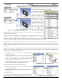
July 6, 2009
The Focus
Issue 70
July 6, 2009
A Publication for ANSYS Users
Issue 70
Changing Names with Release 12
By Doug Oatis
A rose by another any name…blah, you didn’t really think I’d use Shakespeare in one of
my articles, did you? That’s way too high-brow for me. Instead, we’re going with the
Simpsons to discuss name changes at ANSYS R12. In the classic episode, Homer
Simpson changes his name to Max Powers, and gets near instant respect from his boss,
Mr. Burns (who before then could never remember everyone’s favorite Sector 7G employee, learn more here, including the song).
Just like Homer, err, Max’s new theme song, you musn’t fear the new name (“…because
it can be said by anyone”).
Table 1: Name Change Summary
V11 Name
R12 NAME
ANSYS Classic*
Mechanical APDL
Simulation
Mechanical
Project Page
Project Schematic
* Note: It was NEVER officially called Classic, but
it’s what all the cool kids called it.
The name changes at R12 reflect a new commitment to the user and an effort to maintain
a more consistent naming convention with all the recent ANSYS acquisitions. A quick
summary of the name changes is shown in Table 1.
While these name changes don’t appear to do much, the renaming of the
Traditional/Classic ANSYS interface to Mechanical APDL should reassure many users.
There has long stood a fear that the old interface that users had written countless macros
for would eventually go the way of the dodo. Having the name ‘Classic’ was interpreted
as the first nail in the coffin, renaming it to Mechanical APDL is ANSYS’s (Cont. on pg. 2)
The Top 10 Most Important New Features in ANSYS Mechanical APDL R12.0
By Eric Miller
There is a lot to talk about when it comes to new capabilities and features in this recent
release of ANSYS 12.0, and PADT will be spending the next bunch of issues of “The
Focus” digging deep into the ones we think are important. But that is going to take a while
so we decided to start with a “Top Ten List.” (We promise there will be no jokes about
Sarah Palin’s daughter). Based on our readership, we felt that the first place to start was
with our favorites from ANSYS Mechanical APDL, the program formerly,
and incorrectly, referred to as ANSYS In this Issue...
Classic.
1.........Changing Names with Release 12
10: *GET of Participation Factors
This is not earth shattering and will not open up any new more accurate simulations
of exciting and challenging industries. But it is one of those things that has been
frustrating as all heck for years. In the past when you did a modal analysis, you
could only get participation factors by extracting them from the *.out file. This is
doable, but a bit of a pain if you are running batch, but if you are running interactive
you can scroll right past them and they do not get stored in the buffer. The figure
at the beginning of this article shows a modal analysis that put participation factors
in the plot. Download the macro here <LINK>.
1.........The Top 10 Most Important New Features in ANSYS Mechanical APDL
R12
2.........Getting to know R12 Licensing
6.........Navigating the WB 2.0 Project Schematic
10.......About PADT
(Cont. on pg. 4)
www.padtinc.com
1
1-800-293-PADT
July 6, 2009
The Focus
Issue 70
(Names, Cont...)
way of removing that nail. So relax all you APDL power users, your batch-centric mode
of operation is here to stay.
The other name changes aren’t Earth shattering, but may be important when calling your
support provider to tell them where you’re having problems. It should also be noted that
Mechanical APDL and Mechanical should not be confused with the Mechanical license
(ansys increment).
As a last note, I would like to have a moment of silence for the ‘This one goes to 11’
“joke” we used when discussing V11. I can personally attest to its 15% success rate at
making people laugh. I guess along with employing a large group of left-handed people,
PADT also employs the majority of ‘Spinal Tap’ fans. It was good while it lasted, but fear
not, I’ll compensate with even more obscure cultural references.
Getting to Know R12.0 Licensing
By Ted Harris
The licensing scheme has changed a bit at ANSYS 12.0. While the license files are
essentially the same and FLEXlm is still used to allow the licenses to 'float' within a
network, there are a couple of changes that users and license administrators should be
aware of. Primarily, new license manager software needs to be installed on the license
server machine before ANSYS 12.0 can be activated. Other changes include some new
license tasks at version 12.0.
The ANSYS Licensing Interconnect
First, the new ANSYS 12.0 license manager involves software called the ANSYS Licensing Interconnect. This gets installed when the 12.0 version of the ANSYS license
manager is installed on the license server computer. The ANSYS Licensing Interconnect
software is required in addition to the traditional FLEXlm software for nearly all ANSYS
applications to run at version 12.0. Unlike prior versions of ANSYS, the client machine
no longer contacts FLEXlm directly for license communication. At 12.0 the client
contacts the ANSYS Licensing Interconnect, which in turn makes contact with FLEXlm.
The purpose of the ANSYS Licensing Interconnect is to allow sharing of a single license
among multiple ANSYS applications by a single user. An example of that would be the
use of a single Multiphysics license for a meshing session as well as a structural solution
along with perhaps a CFX solution. All of this can be accomplished with a single ANSYS
Multiphysics license. With Workbench 2.0 the processes are all linked and the license is
switched from one application to the next as needed. The ANSYS Licensing Interconnect
allows for this sharing of the license to be much faster than would be possible with just
the FLEXlm component of the license administration.
When the ANSYS 12.0 license manager software is installed on the license server
machine, it will remove any previous versions of the ANSYS license manager software.
Also, for Windows servers, the FLEXlm LMTools utility is no longer available for
ANSYS license administration. Instead, the new Server ANSLIC_ADMIN Utility is the
ANSYS, Inc.-supplied tool to administer the licenses on the server computer.
Finally, note that the ANSYS Licensing Interconnect involves an additional port number,
2325, which must be allowed to pass through any firewall on the network. This is in
addition to the normal ANSYS FLEXlm port (defaults to 1055) and any ANSYS vendor
port that may be added on the server.
(Cont. on pg. 3
www.padtinc.com
2
1-800-293-PADT
July 6, 2009
The Focus
Issue 70
(Licensing, Cont...)
License Administration Choices for the Server
When the ANSYS 12.0 license manager is installed the default choice is to run the ANSYS Licensing Interconnect and FLEXlm
together. This choice will suit most installations, where the ANSLIC_ADMIN utility is used to administer ANSYS licenses.
Alternatively, for companies that prefer to administer ANSYS licenses along with other FLEXlm-served utilities with a non-ANSYS
tool such as FLEXnet Manager, there is another choice in the installation process which allows for the ANSYS Licensing Interconnect
and FLEXlm to run separately. Note that either way, the ANSYS Licensing Interconnect must be installed or it will not be possible to
run the 12.0 version of ANSYS products.
Client (User) License Configuration
On client machines, once ANSYS 12.0 is installed the process to 'point' the client to the server machine is similar to prior versions. The
user runs the Client ANSLIC_ADMIN utility, Specify the License Server Machine option. The client machine is specified along with
the appropriate port numbers.
License Files
Is a new license file needed to run version 12.0? In general, no. As long as the TECS (technical enhancements and support) expiration
date in the license file is later than the release date of ANSYS 12.0 (April 1, 2009), the license file will work with version 12.0.
License Manager Service Pack
Note that a service pack has been released for the ANSYS License Manager for license server as well as client machines. The original
installation may not allow licenses to be shared among applications properly in certain situations. An error message stating that the
licensed number of users has already been reached may appear. The license manager service packs, which includes a complete license
manager installation for the server and an executable replacement for client machines, resolves that problem. In order for the license
server service pack to be installed, the original version should be uninstalled using the instructions provided with the service pack
download, then the service pack should be installed. On the client machines, the required executable needs to be replaced with the new
version.
License Sharing
In order for the aforementioned license sharing for a single user
to work between multiple Workbench 'editors' or modules, the
sharing of licenses among applications must be activated in the
Workbench options. It should be activated by default, but the
settings can be altered by clicking on Tools > License Preferences from within the Workbench project window. The appropriate setting is 'Share a single license between applications
when possible.'
New License Tasks
There are some new license tasks that didn't exist prior to
version 12.0. The main ones involve the new CFD product,
ANSYS CFD. The license task, or name in the license file, for
ANSYS CFD is acfd. This license task allows users to run either
CFX or Fluent. Note that in this case Fluent is labeled ANSYS
Fluent as it's the flavor of Fluent intended to run with the
ANSYS License Manager. A related new license for parallel
processing is ANSYS CFD HPC, which has a license task of
acfd_par_proc. There are several other new license tasks in the
acfd family. The Product Variable Table in the ANSYS 12.0
Licensing Guide lists those, along with all of the other ANSYS
products and their corresponding license task.
For More Information
The ANSYS 12.0 Licensing Guide has extensive documentation
on the license manager, its installation, usage, and troubleshooting. There are also some FAQ's available on the Fluent User
Services Center (yes, they apply to the ANSYS License Manager) at https://secure.fluent.com/sso2/login.htm. You will need
your ANSYS Customer Portal login to access that link.
PADT’s Training Schedule
Month
Start
End
#
Jul
7/7
7/8
104
ANSYS WB Simulation – Intro
Albq., NM
7/9
7/10
205
ANSYS WB Simulation Dynamics
Albq., NM
7/13
7/14
801
ANSYS Customization with APDL
Aug
Sep
Oct
Title
7/20
7/21
203
Dynamics
7/23
7/24
102
Introduction to ANSYS, Part II
Location
Tempe, AZ
8/3
8/4
104
ANSYS WB Simulation – Intro
Tempe, AZ
8/5
8/5
107
ANSYS WB DesignModeler
Tempe, AZ
8/7
8/7
605
CFX for the Non-CFD Specialist
Tempe, AZ
8/10
8/12
152
ICEM CFD/AI*Environment
Tempe, AZ
8/13
8/14
202
Advanced Structural Nonlinearities
Tempe, AZ
8/17
8/18
501
ANSYS/LS-DYNA
Tempe, AZ
8/20
8/21
701
Optimization & Probabilistic Design
Tempe, AZ
8/24
8/25
604
Introduction to CFX
Tempe, AZ
8/26
8/26
112
Meshing for CFX
Tempe, AZ
8/27
8/27
111
ANSYS WB DesignModeler for CFX
9/3
9/4
301 Heat Transfer
Tempe, AZ
Tempe, AZ
9/8
9/11
802 Advanced APDL and Cust.
Tempe, AZ
9/14
9/16
101 Introduction to ANSYS, Part I
Tempe, AZ
9/17
9/18
102 Introduction to ANSYS, Part II
Tempe, AZ
9/21
9/22
201 Basic Structural Nonlinearities
Tempe, AZ
9/23
9/24
204 Advanced Contact and Fasteners
Tempe, AZ
9/25
9/25
653 CFX Turbulence Modeling
9/28
9/29
104 ANSYS WB Simulation – Intro
Las Veg., NV
Tempe, AZ
10/5
10/6
302 WB Simulation Heat Transfer
Tempe, AZ
10/7
10/8
205 ANSYS WB Simulation Dynamics
Tempe, AZ
10/9
10/9
107 ANSYS WB DesignModeler
Tempe, AZ
10/13 10/14
100 Engineering with FEA
Tempe, AZ
10/15 10/16
651 CFX Combustion and Radiation
Tempe, AZ
10/19 10/21
902 Multiphysics Simulation for MEMS
Tempe, AZ
The Focus is a periodic publication of Phoenix Analysis & Design Technologies (PADT). Its goal is to educate and entertain the worldwide ANSYS user community. More information on this publication can be found at: http://www.padtinc.com/epubs/focus/about
www.padtinc.com
3
1-800-293-PADT
July 6, 2009
The Focus
Issue 70
(Top 10, Cont...)
The command is a standard *get:
*get,parm,MODE,n,PFACT,,DIREC,dir
You specify the parameter to store in (parm), the mode you want the factor for(n) and the global direction (dir) which can be
X,Y,Z,ROTX,ROTY,ROTZ. We recommend you store the values in an array. Here is a sample APDL code fragment that works well:
nmd = 10
*dim,pfct,,nmd,6
*dim,adir,char,nmd
adir(1) = 'X','Y','Z','ROTX','ROTY','ROTZ'
*do,i,1,nmd
*do,j,1,6
*get,pfct(i,j),mode,i,pfact,,direc,adir(j)
*enddo
*enddo
9: Four Noded Tets
One of the first things I learned when tet meshers became common was that you should never use 4 noded
tetrahedral (tet) elements. They were too stiff, especially when distorted. Well that is still true for most 4 noded
Tets but when you do large deflection non-linear simulation with 10 noded Tets you often run into problems
where the mid-side nodes fold in to the Tet and cause the dreaded “error in element formulation” error.
ANSYS’s solution, the new SOLID285, is a 4-noded Tet with mixed u-P formulation. It has the
standard three DOF’s at the corner nodes (UX, UY, UZ) and also three internal DOF’s that get
condensed out. The shape function is linear. As you would expect, it does not perform well in
bending and the User Manual actually says “The element may not offer sufficient accuracy for
bending-dominant problems, especially if the mesh is not fine enough.” But, it does perform well for
situations that do not have a lot of bending but see large deflections. This feature is important, but not in the top 5
because its application is somewhat limited.
8: Performance Enhancements to Modal Superposition
In the past, if you had a large model and you wanted to do some sort of modal superposition or PSD things
could sometimes get slow. So ANSYS, Inc. took a look at the whole process and made some changes
under the hood. One of the most significant was to store the eigenvectors (shapes for each mode)
in the .MODE file in node order. Why is this important? Well in the past the information was
simply extracted from the .RST file. But the calculations require the deflection for a given node
across all the modes at the same time. So the program had to “skip” through the .RST file looking
reading the value for each mode for a given node. Now, that info is
written in the .MODE file in node order, so all the values for every solved mode
are grouped together by node in the file – making the reading of that information much faster.
Another speed up is the ability to reuse the stress results from the modal analysis if you expand the
stresses. And lastly, if you are doing a PSD with only single point base excitation, the program no
longer does a static solution as part of the solve. This is required for multi-point excitation and
was therefore done in the past, but now the program checks and skips it if it can. These are very
welcome changes!
7: New Help Viewer
This may be the one controversial choice on this list. I’ve taken a lot of grief from experienced users for supporting this change, but the
more I use it the more I like it. This new release contains a Java based help viewer that is more modern, has powerful search capabilities
and can support help for the entire ANSYS, Inc. product line. It is however different and
some capabilities have gone away… so there are more than a few users here at PADT that
curse when using the new help. But, after you get used to it you can find things faster. It will
also support the continued growth of ANSYS products over time with one consistent viewer
for all products.
6: APDL Math
If you work in a company that has a few seats of NASTRAN, or like us try to sell NASTRAN
users ANSYS, you know that one of the things that NASTRAN diehards cling to is a module
called DMAP. This is a way to stop a solution, extract matrices, modify or add (Cont. on pg. 5
www.padtinc.com
4
1-800-293-PADT
July 6, 2009
The Focus
Issue 70
(Top 10, Cont...)
to them, put them back into the solver and continue on with the solve. ANSYS is taking its first steps in this area with the introduction
of a beta feature called APDL math. It is still not finished and requires a lot of user input before it is done, but is an important first step.
Look for more information on this in future issues of The Focus as we learn more ourselves.
5: General Axisymmetric Elements
These new elements didn’t make the first set of lists because we had not gotten a chance to really explore them fully. But now we have
and we see a lot of potential with the new SOLID272/273 for simulation of rotating stuff. The way they work is that you define a 2D
mesh on any plane (yea! Not just XY anymore with X radial) defined by a local CSYS, which also defines the
rotational axis. Next you specify the number of nodes you want tangentially and generate the elements. This
gives you a 3D representation and nodes that you can apply loads and constraints to (yea! No more
real/imaginary harmonic stuff). It can also be used to transmit torque. So if you have axisymmetric geometry but non-axisymmetric loads, or you have more than one axisymmetric
part that do not share a common axis, these elements are worth checking out.
4: Programmers Manual Available On-Line
Again, not a major deal that is going to change the way people do simulation,
but a change that makes a lot of sense and most importantly, shows ANSYS,
Inc’s commitment to advanced users. In the past if you wanted to learn about
customization and user routines, you had to purchase the Programmer’s manual,
which was often several releases out of date. That manual is now available as
part of the help system and everyone has access to it. If you never looked at it before, you should. It covers a lot of very powerful ways
to expand the program’s capabilities.
3: New Modern Pipe Elements
It can sometimes be hard to get excited about pipe elements unless you do a lot of simulations that involve pipes. But the older pipe
elements in ANSYS were starting to show their age, even though they started out as workhorse elements in early versions of the program.
With PIPE288/289 and ELBOW290, the new modern element formulations have been used to create
these very capable elements. They include features such as: non-linear formulation that is consistent
with all new generation elements, plane stress or full 3-D representation, cubic shape functions
(PIPE289), 3D visualization, and greatly improved hydrodynamic loading.
The elbow is for modeling curved pipes and uses shell theory and Fourier functions to allow the cross section
to distort. It also supports composites (multiple layers) and all of the features found in the PIPE288/289. Even
though it is called an elbow, you can use it to model straight pipe segments that have layers or undergo loading that may
cause the cross section to distort.
2: Contact Enhancements
Generalized contact has changed the way most people do FE modeling and analysis, and with
each release it gets more useful and more general. At R12 a lot of work went into increasing
the efficiency of contact simulation and adding functionality. The change that will benefit
most users are the enhancements to performance, including: , a new search algorithm, not
storing "far field" contact status, and faster computation of contact assembly and results.
Another change that will be awesome for people that need it is the addition of a fluid pressure-penetration load. Basically, this allows
you to specify a pressure on both sides of a contact surface and when the contacts open, the pressure gets
applied. This is a quick way to model a pressurized fluid penetrating the opening and forcing the parts apart.
Beyond these two big changes, there is also: the ability to define friction in terms of two independent fields
(temp, time, pressure, sliding distance, sliding velocity, etc..) instead of just one, a new userfric.f routine that
is much easier to use than the old set of routines, and debonding that has been expanded to cover all of the
different types of bonded contact, not just “Always Bonded.”
1: General Solver Speedup
Everyone wants things to go faster, and users expect to see improvements in every release. But in R12 there
have been a lot of significant enhancements that are worthy of making this our number one choice, because
time is money. Almost every area of the code was looked at and tweaked in some way to get things faster,
and some are mentioned above. There is a whole section in the release notes (2.7) dedicated to all the
(Cont. on pg. 6
www.padtinc.com
5
1-800-293-PADT
July 6, 2009
The Focus
Issue 70
(Top 10, Cont...)
changes – too many to list here. But summed up, we are seeing noticeable improvements in most solves that we are doing, and usually
less memory. This is a change that will benefit everyone.
As mentioned at the top, this is just a quick overview of the to 10 things that PADT thinks are important in ANSYS Mechanical APDL.,
and in the next issue we will share our thoughts on the most important changes to the Workbench side of things. But do not take our
word for it. Take a look at the release notes, review PADT’s R12 seminar PPT’s or attend a seminar with ANSYS, Inc. or your channel
partner. There is a lot of good stuff there waiting for you to find it.
Useful R12 Resources:
ANSYS, Inc. Website:
New Issue of ANSYS Advantage:
ANSYS R12 Tutorials, PowerPoints and FAQ:
PADT’s R12 Seminar PowerPoints:
www.ansys.com/products/ansys12-new-features.asp
www.ansys.com/magazine/default.asp
https://www1.ansys.com/customer/content/ansys12.asp
ftp.padtinc.com/public/seminars/2009_06_10_R12_NewSTuff.zip
Navigating the WB 2.0 Project Schematic
By Jeff Strain
You, an ANSYS user who, while quite experienced with the "Classic"
interface, have also explored the Workbench products extensively to ensure
you're taking full advantage of the analysis tools at your disposal. After
several hours of downloading and installing the ANSYS 12.0 release, then
going back and forth with tech support before realizing that you have to
install the new license manager too, you find yourself salivating like Mark
Sanford in a Buenos Aires tango club as you launch Workbench 2.0 for the
first time. As the splash screen gives way to the application, you're greeted
by a large blank field with a list of analysis types perched to the left. It's
nothing you've ever seen before.
Pausing, you contemplate the flask of bourbon residing in your hollowedout Marks handbook. However, once you examine the Workbench 2.0
Figure 1: Well, this is Different!
capabilities, you'll appreciate its advantages, including its process-centric
approach, its physics neutral format, its ability to share common utilities across applications, its multiphysics capabilities, its global
parameter manager, etc.
The Workbench 2.0 interface consists of two main windows: the Toolbox and the Project Schematic. The Toolbox consists of complete
analysis applications, such as static structural, transient thermal, and fluid flow analyses. These applications include material
properties, geometry, mesh, boundary conditions, and results. All of these are found under Analysis Systems. There are also
component systems consisting of stand-alone tools, such as
geometry creation and CFX postprocessing.
Any of these Toolbox objects may be inserted into the Project
Schematic. The Project Schematic is where modules and
analyses are managed. To insert a Toolbox system into the
Project Schematic, simply double-click or click and drag the
desired system into it. Figure 2 shows a Static Structural
Analysis.
Note that the analysis system is organized in a column of
spreadsheet like cells. It is from these cells that each aspect
of the analysis is controlled. In this case, Engineering Data
provides access to the material properties. The Geometry
cell can be used to launch DesignModeler, import a saved
CAD file, or attach an active CAD model. (Cont. on pg. 7)
www.padtinc.com
Figure 2: Static Structural Analysis Schematic
6
1-800-293-PADT
July 6, 2009
The Focus
Issue 70
(Schematic, Cont...)
The Model, Setup, Solution, and Results cells all control meshing,
boundary condition application, solution settings, and results viewing in Mechanical, formerly know as Simulation .
Note the symbols to the right
of each cell. A check mark
( ) indicates that a cell is
completely defined. (Be
aware that, as before, the
Mechanical material defaults
to structural steel.) A question mark ( ) indicates that
data needs to be defined (e.g.
geometry needs to be attached or created). The circling arrows ( ) indicate
that a cell needs to be refreshed (e.g. a model needs
to be refreshed to reflect
Figure 3: Accessing Workbench Modules
changes in geometry). A lightning bolt (
solution needs to be performed).
) indicates that the cell needs to be updated (e.g. a
To launch a module, simply double-click the appropriate cell or right-click and select Edit. For
example, to launch DesignModeler, double-click the Geometry cell.
To launch
Mechanical/Simulation, double-click the Model cell within the Static Structural analysis system. Figure 4: Geometry Properties
Once you're within the geometry and analysis modules, the interface is almost the same as in version 11.0.
Each cell has a set of properties associated with it, such as geometry import options or solution settings. Though the properties are
hidden by default, it's recommended that you turn them on by clicking View > Properties since they provide a relative unobtrusive
method of viewing and adjusting your cell settings. When turned on the Properties window may be found on the right side of the Project
Schematic.
So what's the deal with this spreadsheet layout? Note that the cells are all referenced in their corresponding locations within the modules
(Figure 5). The spreadsheet organization also provides the structure for linking cells and systems for sharing and transferring data.
These linkages enable the following capabilities:
· Sharing specific data, such as geometry or material properties,
between applications.
· Providing initial condition or prestress data for analyses, such as
prestress modal analysis (static -> modal), random vibration
(modal -> random vibration), or transient thermal initial conditions (steady state -> transient thermal)
· Enabling coupled-field analyses, such as thermal-structural, fluidstructural interaction (FSI), and conjugate heat transfer.
Figure 5: Analysis Cell References
To share individual analysis components (see Figure 6):
1: Make sure that all analysis systems of interest have been inserted
into the Project Schematic.
2: Drag and drop the data to be shared from the origination cell to the
destination cell.
3: Repeat as needed.
To transfer data for initial conditions or coupled field analysis, rightclick the Solution cell of the originating analysis, select (Cont. on pg. 8)
www.padtinc.com
7
Figure 6: Sharing Cell Data
1-800-293-PADT
July 6, 2009
The Focus
Issue 70
Figure 7: Thermal-Stress Schematic
(Schematic, Cont...)
"Transfer Data To New >" and select the appropriate analysis from the flyout menu. For example, to apply steady state thermal results
as structural temperatures, right click the Solution cell in the Steady State Thermal analysis system and select Transfer Data To New >
Static Structural (ANSYS) as shown in Figure 7. Note that the Custom Systems list already contains a number of pre-defined initial
conditions and coupled-field setups, which may save you some effort.
Note that each link has a square or a circle at the end. The square indicates that data is shared between systems. In Figure 7 both thermal
and structural models have the same materials, geometry, and mesh. A circle at the end of a link indicates that data is transferred from
one cell to the other. In this same figure the resulting steady-state temperatures from the thermal model are applied as structural
temperatures in the static structural model.
As before, it is possible to solve each analysis separately within its respective module. However, clicking the Update Project icon
(
) will update each module as applicable and solve all models throughout the schematic. A typical analysis approach
within the Workbench 2.0 interface would be to set up meshes and apply loads within their respective modules, then solve all analyses
by updating the entire project.
With the Project Schematic, there is no limit to how many cells can be linked and how many analyses can be coupled together. For
Figure 8: Seriously, you can go nuts with this thing!
instance, the schematic not only provides a simple method of conducting thermal-stress or conjugate heat transfer analyses, you can also
use the resulting temperatures from a conjugate heat transfer analysis as thermal loading in a structural analysis and so on.
The new Workbench Project Schematic reflects a migration to Workbench 2.0 and is therefore a Workbench native application. On the
other hand, DesignModeler, Mechanical and other modules are still at Workbench 1.0 though they are Workbench 2.0 compliant. In
addition to the Project Schematic, Engineering Data and the Parameter Manager have been updated to Workbench 2.0 native format.
Eventually, all Workbench modules will be upgraded to 2.0 and capabilities will continue to be consolidated.
(Cont. on pg. 9)
www.padtinc.com
8
1-800-293-PADT
July 6, 2009
The Focus
Issue 70
(Schematic, Cont...)
In R12.0, the Engineering Data only consists of
material properties. Load data is managed in individual applications. This will change in future applications as Engineering Data eventually incorporates
all of the data it contained previously. The new
Engineering Data tool exposes all material data in a
single level, such as tabular properties, material data
charts, libraries, current materials, and so forth. The
interface is managed by incorporating the Workbench 2.0 paradigm of dropping predefined toolbox
items into the model.
The Parameter Manager has also been updated to
Workbench 2.0 format and acts as a global parameter
manager for all of the Workbench modules. Exposing a parameter in an application automatically sends
it to the Parameter Manager. The Parameter Manager can be used to conduct what-if studies between
input and output variables. It also allows the user to
perform mathematical operations between parameters, among other capabilities. Like the Engineering
Data tool, it contains windows for tabular input and
output as well as x-y charting capabilities. To return
to the Project Schematic from Engineering Data, the
Parameter Manager or any other Workbench 2.0 tool,
click on the Return to Project button (
).
Figure 9: Engineering Data in WB 2.0
Rather than individual database files, the entire
Workbench project is saved. The file structure consists of a master project file (.wbpj) and a series of
associated subfolders containing the modeling databases and analysis files. Since the file structure is so
complex, Workbench projects should be transmitted
Figure 10: Parameter Manager in WB 2.0
by first archiving the project to a zip file (File >
Archive) and then unarchiving the zip file (File > Restore Archive) when it reaches its destination. You may view all of the files
associated with a project and their descriptions by clicking View > Files.
Additional details about Workbench 2.0 tools such as Engineering Data and the Parameter Manager will be covered in more detail in
future Focus articles. Also look for articles discussing Workbench project file management. ANSYS Inc. has put significant effort
smoothing the transition to Workbench 2.0 by making a number of tutorials available at their customer portal, which you may find at
www1.ansys.com/customer .
News - Links - Info
· Two Time America’s Cub Winner Alinghi Chooses ANSYS Products to Help Defend the Cup <link>
· ANSYS offers free link to CHEMKIN-CFD chemical solver for FLUENT users, a must have for people modeling
chemical reaction in their flow models <link>
· Ansoft side of things release new version of SiWave, software for signal integrity, power integrity and electromagnetic
compatibility testing <link>
· A couple of great issues of the ANSYS magazine have been published since the last The Focus <link>
www.padtinc.com
9
1-800-293-PADT
July 6, 2009
The Focus
Issue 70
In the past we have finished up The Focus with a page we called “Shameless Advertising...” The truth was that the page was really
only advertising PADT, and PADT related things. So, instead of doing advertising we thought we would just dedicate the final page
to explaining who PADT is, what we do and how we can hopefully help you. And, to make sure you read it, we will try and stick
something funny in. Want to know more? Call Stephen Hendry at 207-333-8780 or e-mail [email protected].
What is PADT’s Business:
PADT is dedicated to synergistically bringing leading edge resources to win-win customer-vendor partnerships to enable success in
mission critical situations. Blah... Blah... Blah (actually, that is not far off from the text on a booth a show we recently attended, yuck!)
Getting serious now, we are company with a little over 50 engineers, technicians, sales people, business-task-doers, and infrastructure-keep-things-running-guys, who provide hardware, software and technical services to companies who make mechanical products.
We do this by having three departments whose staff focus on one of three areas: Numerical Simulation, Product Development and
Rapid Manufacturing. We work in almost any industry, and around the world.
Many perspective customers ask us how we have been able to grow over the past 15 years and keep such a loyal customer following.
We would like to say we have a snazzy mission statement that everyone works by, but in reality we just try to follow the core
principals that we founded the company with:
Ÿ Establish a high level of integrity
Ÿ Use the best people
Ÿ Learn your tools inside and out
Ÿ Synergistically combine disciplines
Ÿ Provide flexible solutions of a higher quality in less time for less money
It is that simple. We are run by a bunch of engineers and anything more complex or sophisticated would be too hard to remember,
and more importantly, go against our inner “nerds”.
Come back to this page over the next couple of issues to learn more about each of PADT’s departments and maybe we can work
together in the future.
PADT on the Web
Need ANSYS Help?
Besides our home site, PADT has many other locations on the web
to promote specific products or services:
www.PADTINC.com PADT’s main website
www.PADTMedical.com Medical device development
www.DimensionSCA.com A machine that PADT makes
www.uPrintStore.com A place to buy 3D Printers & Supplies
www.XANSYS.org ANSYS User forum
PADT can help in many different ways, here are a few:
Ÿ We hold training here or at your facility <link>
Ÿ Leverage our APDL knowledge with the APDL Guide <link>
Ÿ Consider one-on-one support through mentoring, a great
way to get a quick start on something new <link>
Ÿ Attend a PADT Webinar <link>
A Free Joke:
A lead hardware engineer, a lead software engineer, and their program manager are taking a walk outdoors during their lunch break
when they come upon an old brass lamp. They pick it up and dust it off. Poof -- out pops a genie.
"Thank you for releasing me from my lamp-prison. I can grant you 3 wishes. Since there are 3 of you I will grant one wish to each of
you."
The hardware engineer thinks a moment and says, "I'd like to be sailing a yacht across the Pacific"
"It is done", said the Genie, and poof, the hardware engineer disappears.
The software engineer thinks a moment and says, "I'd like to be riding my Harley across the American Southwest."
"It is done", said the Genie, and poof, the software engineer disappears.
The program manager looks at where the other two had been standing and rubs his chin in thought. Then he tells the Genie, "I'd like
those two back in the office after lunch."
www.padtinc.com
10
1-800-293-PADT