Download Traxtile User Manual

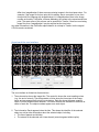
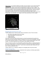
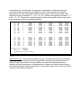
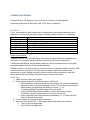
Traxtile User Manual
Copyright © 2014, The Regents of the University of California. All rights reserved.
Developed by Benjamin S. Braun MD, PhD; UCSF Dept. of Pediatrics
Installation
To run, download the Python modules into a single directory, and sample data (often into a
subdirectory, but this is not necesary), and run 'traxtile.py' with the Python 2.7.x interpreter.
ImageViewer.py
MontageFile.py
Trax_io_icy.py
Trax_io_isbi.py
Trax_io_trackmate.py
MontageView.py
Trackmodel.py
traxtile.py
Module for „whole image‟ view
Module for import/export and reporting operations
Import Icy/TrackManager data
Import ISBI Challenge 2012 format data
Import Fiji/TrackMate data
Module for main program interface
Module for data model
Main program
System Requirements:
Software: Python 2.7.x is required (earlier versions do not support dictionary comprehension
and Python 3.x and above require alternative syntax for some iteration operations).
Traxtile was developed on the Mac platform (Mac OS 10.8.5) but should work on any Python
compatible platform with only Python standard libraries.
Hardware: Memory is a limiting resource, since the entire list of objects is helpd in memory. 2GB
is recommended as a minimum, but larger amounts may be required for medium sized
experiments or larger. Multiple processor cores are unlikely to speed execution. Hard disk
assess time may be rate limiting; solid state memory drives can be helpful.
Quick Start
1. Obtain a series of time lapse images
2. Perform object recognition and initial tracking in CellProfiler
 Save at least one processed version of each image in GIF format in a dedicated
directory or folder, using the SaveImage module. The file name must include the
frame number in 4-digit string; the default is to follow “_t” e.g.
“timelapse_t0123.gif” would be image #123 in the series.
 Use the IdentifyPrimaryObjects module to identify the objects, and the
TrackObjects module to track them from one frame to the next
 Export Image Data and Object Data as spreadsheets (i.e., csv files) using the
ExportToSpreadsheet module
3. Launch Traxtile. An empty workspace will appear.
4. Select the „File / Import CSV…‟ menu option and use the dialog box to identify:
 The CSV file with image data
 The CSV file with object data

The columns in the object data file that indicate the Parent Group, Parent Object
and Frame number. Defaults will be selected automatically, but the specific
names of these columns may vary since they are chosen by CellProfiler using
experiment specific metadata.
 The location of image files to use in the tiles
 The location of image files to use for the „whole image‟ viewer. These may
optionally be the same as the tile images.
 Press “OK.” Traxtile will load and process the data, and the tile viewer will fill with
images around the first sentinel event (object spit, merge, appearance or
disappearance)
5. Edit objects and tracks
 Select a cell by clicking on its number
 Make or destroy connections to the selected object by ⌘-click or Alt-click
 Remove the selected object using the Delete key
 Create new objects using Control-click
 Move through the list of events using the left and right arrow buttons
6. Create reports using the „Analyze‟ menu
7. Save data in binary format („File / Save…‟) or CSV („File / Export CSV…‟)
.
Required elements for CellProfiler data
The following data sources are required to run Traxtile:
1. A comma-separated values (csv) file with object data, created by CellProfiler using the
ExportToSpreadsheet module.
2. A csv file generated by CellProfiler with image data.
3. Images to be used for the montage tiles. These must be in GIF format, and are often saved
at some point in the CellProfiler image processing pipeline. These files must have the same
pixel dimensions as the images used in the IdentifyPrimaryObjects module. The file name
must include a 4-digit number to indicate the time point for the image (also called time index
or frame index). Apart from this 4-digit number, the file names must be identical.
4. Optionally, a separate series of image files to be use for the Image window view. These also
must be in GIF format, have the same pixel dimensions as the images used in
IdentifyPrimaryObjects, and have names that differ only by the 4-digit time index.
The following columns are required in the object data file:







ImageNumber
ObjectNumber
Location_Center_X
Location_Center_Y
ParentImageNumber, or any column that indicates the image number of an object‟s
„parent.‟ This is usually the preceding image, but it can be further removed if there is a
gap at this point in the track. The exact name of this column can be specified in Traxtile.
ParentObjectNumber, or any column that indicates the parent‟s object number. The
exact name of this column can be specified in Traxtile.
Metadata_time, or any column that holds the time index (i.e., the number indicating the
time point in the series). This column will only be present if the ExportToSpreadsheet
module in CellProfiler is configured with the option to “add image metadata columns to
your object data file.” In addition, the time index must be derived from the original image
loaded by CellProfiler, so that it is included in the image metadata. The time index may
differ from ImageNumber if there are some missing images in the time lapse series. For
example, if the image file for time point #14 is missing, due to corruption or loss, then
time point #15 will appear with ImageNumber #14. ImageNumber refers to the image
number as found by CellProfiler, whereas Metadata_time refers to the experimental time
point. The exact name of this column can be specified in Traxtile. If there are no missing
image files, then “ImageNumber” may be selected as the time index.
Any other information in the CellProfiler object data file is not kept in Traxtile, but the original
CSV file remains unaltered.
Overview of the user interface
Figure 1
The user interface is divided into three sections:
1. The main section shows the image tiles. The center tile shows the event needing review
(e.g., the end of a track). Tiles that precede or follow show the time steps of the image
series and are arranged left-to-right, top-to-bottom. Each tile shows the same cropped
region, but with different frame numbers. The frame numbers are indicated in the lower let
corner of each tile. The object numbers appear over each object.
2. The Information Panel appears below the tiles. This shows the identifier of the selected
object, as well as other information about the selected object, including:
 The lists of parents and children
 The extents of the selected cell‟s linear branch (a track segment without splits)


The roots and tips connected to the selected cell
If the selected cell is a tip, it may be categorized as a Death or Disappearance (loss of a
cell from the imaging without death, e.g. by migration out of view)
The object identifier consists of the frame number, follwed by a hyphen, followed by the
object number in that frame. Object numbers are assigned by the CellProfiler
IdentifyPrimaryObjects module. Note that, because these are assigned for each image
before object tracking, object numbers can change from one frame to the next as objects
move, appear and disappear.
3. The Navigation Panel on the bottom provides buttons for moving through the list of reviewed
events.
Loading and Saving data
Importing data from CellProfiler
The “File / Import CSV…” menu option brings up the following dialog box:
The required information is:
CSV file for Image information
The image data file created in CellProfiler using ExportToSpreadsheet. Select a file using
the “Browse” button.
CSV for Object information
The object data file created in CellProfiler using ExportToSpreadsheet. Select a file using
the “Browse” button.
Field name for Parent Image Number
The exact name of the column holding the image number for an objects „parent,‟
corresponding to ParentImageNumber above. Traxtile will attempt to find a column whose
title includes the word “ParentImageNumber” and use this as a default. However, all the
columns in the file are available using the selector.
Field name for Parent Object Number
The exact name of the column holding the object number for an objects „parent‟ within its
own image, corresponding to ParentObjectNumber above. Traxtile will attempt to find a
column whose title includes the word “ParentObjectNumber” and use this as a default.
Field name for Time Index
The exact name of the column holding the time index for each object (also called a frame
index), as described above for Metadata_time. Traxtile will attempt to find a column whose
title includes the word “Time” and use this as a default. If image metadata is not stored, and
if no files were missing during the CellProfiler run, then “ImageNumber” may be selected
here.
Images to use for display
Traxtile requires time series images to display in tiles. Optionally, a second set of images
can be used for the Image viewer window, though it is common to use the same images for
both displays. All the images for each purpose must be in a single directory. To fill these
fields, press the “Browse” button, navigate to the proper directory, and select any one of the
image files in that directory. Traxtile will inspect the file name and attempt to separate it
into discrete components:




Prefix:
Image #:
Suffix:
Extension:
anything preceding the time index
the four-digit number indicating the time index
anything coming after the time index, before the extension
must be .gif
Except for the image #, each of these must be identical for all the images. The default
pattern for the image # is “_tnnnn” where “n” is a digit 0-9.
In the example above, a file named “subtracted_2x_s1_t0001.gif” was selected. The time
index is the four digit number after “_t,” so the prefix is “subtracted_2x_s1_t” and there is
no suffix.
These assignments can be manually edited in the fields provided.
Pressing “OK” will trigger reading the files and constructing the data model. For large
experiments, this may take several minutes. Then the main tile display will open with the first
event‟s object selected.
Importing data from other sources
The following data sources are required to run Traxtile with Icy:
 An XLS file output from the „Spot Detector‟ plugin, converted to CSV format
 An XML file created in the „TrackManager‟ plugin, using the File / Save… option.
 Images in GIF format to be used for the montage tiles and, optionally, the whole image
view. These are described above
The following data sources are required to run Traxtile with Fiji‟s TrackMate plugin or the ISBI
Challenge 2012 format:
 An XML format file created, for example, with the „Save‟ feature in Trackmate
 Images in GIF format to be used for the montage tiles and, optionally, the whole image
view, as described above.
Saving and loading workspace files
The “File / Save…” menu item allows saving a binary format file containing the data model and
configuration information. The default extension is “.txl” but any may be used. Saved files can
be loaded in a later session using the “File / Open…” menu option. Note, however, that image
files must reside in their original location, as the saved file refers to this directory.
Exporting CSV files
The current workspace can also be exported as a “comma-separated values” (CSV) formatted
file that can be re-imported as an object data file later or used for external analysis. For example,
this file could be used to apply survival analysis to deaths as a function of time, with
disappearances as censored events.
Note that this file follows the convention of CellProfiler 2.0, so object merges are not
represented explicitly in the CSV file. Only one parent is listed for each object. For this reason,
to avoid losing merge events from the data set, it is advised to save workspace files in binary
format as well.
Track Editing
The following actions are available for editing tracks:
Object selection. An object is selected by clicking on its identifying number. The number then is
highlighted by color, and the tracks associated with that object appear as lines between tiles.
Object removal. The selected object is removed from the database by either pressing the Delete
key on the keyboard or pressing the Delete button in the center of the Information Panel. When
an object is deleted, its first child is automatically selected. This makes it easy to delete several
linked objects in a track.
There is no „undo‟ function, so deleting an object is permanent. However, a connection can be
made between the deleted object‟s parent and child. In effect, this replaces an object with a gap,
with no net consequence for the track. This is not possible if the deleted object is a root or tip.
Object creation. A new label can be added to the data set using Control-click, i.e. holding the
Control key and clicking with the mouse in the location for the new label. As noted above, cells
are inferred to exist in gaps, so adding cells is often not needed. However, there may be some
cases when a proper timing of a split or death event might require a new object.
Create or remove connections. Editing tracks is the essential purpose of Traxtile. In the example
below, the initial tracking algorithm identified no children for object #64 in frame #27 (i.e., 2764) , so it initially appears as the end of a track. Thus, it is shown as a track „tip‟ and is
highlighted with a diamond:
Figure 2
However, this cell actually moved slightly northeast, and becomes object #56 in frame #28.
(because the tracking algorithm did not discover this link, 28-56 is erroneously designated as a
root, having no parents). To correct this, begin with object 27-64 selected. Then, holding down
⌘(OS X) or Alt (Windows, Linux) on the keyboard, click on #56 in frame #28. This will create
the link, as shown:
Figure 3
Now, there is a single track that includes 27-64 and 28-56. The data set now has one less tip
and one less root.
Connections can be removed the same way. Holding down ⌘or Alt and clicking on a connected
object will remove the link between it and the selected object.
There is an alternative way to do this using the Information Panel below the image tiles. The
parents and children are listed on either side of the slected cell. If you press the button marked
“Unlink Parent,” then the link to the parent that is highlighted in the Parents list will be removed.
If no Parent is highlighted, then the top one is removed.
Figure 4
If the “Add Parent” button is pressed, then clicking on an object in the tiled images will be linked
as a parent to the current object. This is very similar to the ⌘-click / Alt-click action. There is not
a way to manually type in an object identifier to create a link. Children can be linked and
unlinked the same way.
Image window. It is sometimes helpful to be able to see how objects in a given tile have gotten
there, especially if they are moving quickly enough that they appear in only a few tiles. For
assistance, the “Images” window can be opened (Window / Image menu item or ⌘/Alt-I). This
shows an uncropped version of the image containing the selected object. The view is centered
on the selected object, and a highlight box delineates the edges of the tile. Scroll bars can be
used to pan the image. The title of the Image window indicates the image file name.
Importantly, the left and right arrow keys on the keyboard will advance through the image series.
This provides a more dynamic view of object motion than presented by the tile montage.
Figure 5
Navigating the list of events for review
Traxtile compiles a list of “sentinel events” that are selected for review. This list includes:




New objects that appear after the first frame
Tracks that end prior to the last frame
Objects that split
Objects that merge
The bottom of the main window holds buttons for moving forward and back through this list.
When these are used to advance forward or backward, a new set of tiles is displayed, centered
on the event of interest if possible. The object of interest is selected automatically, and its track
is shown. The left and right arrow keys may also be used instead of the buttons.
The list of events for review is not automatically updated during editing, to enable going back to
previously reviewed items for a second look. However, the list can be recompiled by selecting
the “Analyze / Recalculate” menu option. The list is also recalculated when loading a file from
disk or importing CellProfiler data.
A button marked „Go To‟ brings up a dialog box for navigating the list by event number.
Analysis and reporting
A note on modeling population growth. A population that is growing or shrinking exponentially
follows the equation:
( )
With definitions:
(
)
n(t)
n0
e


t
number of objects at time t
number of objects at time zero
base of natural logorithm
birth rate (births per cell per time unit)
death rate (deaths per cell per time unit)
time
The parameter ( - ) is the net growth rate, and it can be estimated in Traxtile by two distinct
methods. First, the birth and death rates can be observed directly from the collection of tracks.
Second, the number of objects in each frame can be used to compute an exponential curve by
linear regression (using the logarithm of obect number). Each of these estimates is subject to
statistical error, so they will not always yield the exact same number. Though beyond the scope
of this manual, these two methods reflect the ability to model population growth using either a
deterministic model, as produced by the regression, or a stochastic Markov birth-death model,
which is informed by the direct observation of events.
There are three reports available in Traxtile, each accessed from the „Analyze‟ menu. A report is
presented as plain text in a spearate window. A report can be saved as text files or copied to the
system clipboard.
The report types are:
Summary. This report describes overall statistics for tracks in the series. This includes the
number of objects present in the first and last images, and the total number of ojects identified
or inferred in all the images. The number of roots and tips is also reported, including those in the
first and last frames; the subset of those chosen for review (i.e., outside the first and last
frames) is also given.
Gains and losses of objects are reported acccording to type, both by total number and by the
normalized rate (per cell per frame). To illustrate how rates are calculated, consider an example
in which 20 objects are followed over 5 frames. A total of 100 objects are observed (20 x 5). If
one of these splits, then the observed rate of splitting is 1 per 100 observations, or 0.01.
Growth modeling predicts that the exponent in the growth equation should be equal to the net
rate of object gains. The observed net rate is also reported.
Finally, gaps are summarized by length. This information can help guide the choice of gap
length parameters when performing object tracking for similar experiments in CellProfiler.
Note that this information reflects the editing and validation performed by the user and therefore
provides a „gold standard‟ that can be useful for optimization.
cells observed:
starting number:
ending number:
12387 (cells x frames)
126
124
Ends:
Roots:
Tips:
Total Reviewing
158 32
160 36
Gains:
splits:
new cells:
Total:
No.
13
32
45
Rate (no./cell/frame)
0.00104948736579
0.00258335351578
0.00363284088157
Losses:
deaths:
disappearances:
merges:
other:
Total:
No.
0
Rate (no./cell/frame)
0.0
0
0.0
0.00088802777105
0.00290627270526
0.00379430047631
11
36
47
Net Rate (gains - losses):
-0.000161459594736
Gaps:
size
1
2
3
4
5
6
7
8
9
10
No.
11936
75
18
9
5
1
3
0
2
1
Figure 6
Counts. A more detailed report lists data for each frame in the series. Each row reports, for one
time point, the numbers of objects (cells) and the cumulative number of splits, newly appearing
objects, losses (i.e., tips) and merges from the beginning of the experiment to the indicated
frame. The rates, as calculated from the start of the experiment to each frame, are also given.
Trends in these calculated rates demonstrate the extent to which estimates have reached stable
values during the course of the experiment. If they are still changing significantly at the end of
the time course, a longer period of observation might be helpful. This is illustrated in the graph
below, which was made by pasting the “Counts” report into Excel. Note that the estimate of cell
division rate is still rather unstable, suggesting that a larger data set (more objects and/or a
longer observation period) might be needed.
SplitRate
0.0012
0.0010
Rate
0.0008
0.0006
0.0004
0.0002
0.0000
0
Figure 7
20
40
60
80
Time index
100
120
At the bottom of the Counts report, the regression results appear, including an estimate of
population doubling time based on the regression model. If the regression fits a negative
exponential curve, then the population half-life is given instead. In the example below, direct
observation yields an estimate of ( - ) of -1.61  10-4, whereas the regression estimates ( - )
to be 1.73  10-5. Though one is a positive number and the other negative, both are very close
to zero, and are not likely to be statistically distinct.
Frame
1
2
3
4
5
6
7
8
9
10
.
.
.
91
92
93
94
95
96
97
98
99
Cells
126
126
126
126
126
126
126
126
126
125
.
.
.
125
125
124
124
124
123
123
124
124
CumCells
126
252
378
504
630
756
882
1008
1134
1259
.
.
.
11396
11521
11645
11769
11893
12016
12139
12263
12387
CumSplits
0
0
0
0
0
0
0
0
1
1
.
.
.
12
12
12
12
12
12
13
13
13
SplitRate
0.000000
0.000000
0.000000
0.000000
0.000000
0.000000
0.000000
0.000000
0.000882
0.000794
.
.
.
0.001053
0.001042
0.001030
0.001020
0.001009
0.000999
0.001071
0.001060
0.001049
CumNew
0
0
0
0
0
0
0
0
0
0
.
.
.
32
32
32
32
32
32
32
32
32
NewRate
0.000000
0.000000
0.000000
0.000000
0.000000
0.000000
0.000000
0.000000
0.000000
0.000000
.
.
.
0.002808
0.002778
0.002748
0.002719
0.002691
0.002663
0.002636
0.002609
0.002583
CumLoss LossRate
0
0.000000
0
0.000000
0
0.000000
0
0.000000
0
0.000000
0
0.000000
0
0.000000
0
0.000000
0
0.000000
0
0.000000
.
.
.
.
.
.
34
0.002984
35
0.003038
35
0.003006
35
0.002974
36
0.003027
36
0.002996
36
0.002966
36
0.002936
36
0.002906
CumMerge MergeRate
0
0.000000
0
0.000000
0
0.000000
0
0.000000
0
0.000000
0
0.000000
0
0.000000
0
0.000000
0
0.000000
1
0.000794
.
.
.
.
.
.
11
0.000965
11
0.000955
11
0.000945
11
0.000935
11
0.000925
11
0.000915
11
0.000906
11
0.000897
11
0.000888
NetRate
0.000000
0.000000
0.000000
0.000000
0.000000
0.000000
0.000000
0.000000
0.000882
0.000000
.
.
.
-0.000088
-0.000174
-0.000172
-0.000170
-0.000252
-0.000250
-0.000165
-0.000163
-0.000161
Fitted growth curve n(t) = n0 * exp(a * t):
n0:
125.007696
exponent (a):
1.72979e-05
population doubling time: 40071.110188 frames
Figure 8
Newick tree format. There are several formats used to encode tree-like structures. The Newick
format is one such schema that is widely recognized by tree drawing programs available for
Python, R, and other platforms. The set of tracks in an experiment can be reported as a
collection of Newick-format trees, as illustrated below. However, note that the Newick format,
which was developed to describe phyolgenies in evolutionary biology, does not have a standard
notation for the merging of branches.
((99-32:18,99-20:18)81-25:2,99-23:19)79-23:1;
(99-121:23,99-115:23)76-115:76;
(99-13:67,99-38:67)32-19:32;
(99-34:69,60-31:30)29-23:29;
(99-62:17,99-59:14)82-58:37;
(85-58:29,99-65:43)56-56:56;
(99-79:53,99-71:53)46-78:46;
(99-62:17,99-59:14)82-58:37;
(99-70:16,99-84:16)83-81:15;
(99-70:16,99-84:16)83-81:15;
(26-79:3,99-27:72)23-72:23;
(99-46:14,99-53:14)85-48:7;
(99-26:2,99-36:2)97-26:97;
99-100:99;
99-123:99;
99-120:99;
99-124:99;
99-102:99;
99-107:99;
99-103:99;
99-114:99;
99-105:99;
99-110:99;
99-111:99;
95-100:95;
99-109:99;
99-119:99;
Figure 9