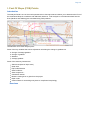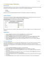
1
SHELF
Tutorial Collection
© Copyright by Geocap AS
Printed April 2013
Page 1
Shelf (UNCLOS Art. 76) Tutorial
This tutorial collection is specific to UNCLOS article 76 functionality in Geocap. The Atlantis project will be used
as an example project, but other projects may be used instead when doing the exercises. The order of the
tutorials more or less describe the order in which a real project would be done.
Content
Page
A.
Getting Started with Geocap Shelf
2
B.
Geocap Interface
5
C.
Create a New Shelf (UNCLOS) Project
13
D.
Import and Export
15
E.
Baseline Generation (Simplified)
18
F.
Bathymetric Grids And Generation Of Bathymetric Profiles
20
G.
Generation Of Distance Lines And Mid-Lines
23
H.
The Analysis Panel
27
I.
Foot Of Slope (FOS) Points
28
J.
Real Bathymetric Profiles
32
K.
The 2500m Isobath
33
L.
Seismic Interpretation
35
M.
Depth Conversion
39
N.
Sediment Thickness
43
O.
Final Outer Limits
47
P.
Uncertainty
50
Q.
Gridding
52
R.
Plotting
54
S.
Workflows
55
T.
Image Georeferencing
58
U.
Vertical Image Calibration
61
Z.
Additional Shelf Exercises
63
Page 2
A. Getting Started with Geocap Shelf
Introduction
Geocap is a software for visualization and manipulation of geodata. The core features of Geocap are:
2D/3D visualization of any geodata in the same graphics window
Gridding
Plotting
2D seismic and interpretation
Geodetic conversion
Image georeferencing
Workflows
GIS
Scripting
On top of these features Geocap provides a set of plugins that fit perfectly in to your line of work:
Shelf - for continental shelf delineation in accordance with UN Convention on the Law of the Sea, Article
76.
Seafloor - for processing survey data from multibeam echo sounders,
Oil & Gas and GIM - for oil exploration and reservoir modeling.
Your Geocap installation will consist of the basic Geocap platform and one or several of these plugins.
Exercises:
Start Geocap
Open Geocap from the main Windows Start Menu > All Programs > Geocap.
Starting Geocap from the startmenu
User Documentation
Parts of the user documentation is found under the Help pulldown. There rest is found here: http://www.geocap.
no/doc. Read briefly through the documentation to get an understanding of what you can expect to find in the
documents.
The user documentations consists of:
User Guide with detailed descriptions of Geocap usage.
Reference manual with syntax and details of the commands in the Geocap scripting language.
Page 3
Installation Guide with details on installation, dongle drivers etc.
Release Notes contains incremental updates and bug fix descriptions as well as major releases.
Articles is a collection of articles on various topics that still is not included in the documentation.
Tutorials contains thematic tutorials on products. The General tutorials mainly contains topics that are
put in a better context within the more specialized product tutorials.
FAQ is a list of Frequently asked questions, with their corresponding answers.
Geocap Extensions contains different scripts and add-on functionality for Geocap.
The Options dialog
The Options dialog lets you define what Geocap should do on startup. This means that you can predefine a
background color, working directory, data window and automatic loading of plugins and scripts etc.
Exercise
Explore the different settings in the Option dialog
Open the dialog by going to Tools > Options
Go down section by section and make sure you understand the meaning of each of them
Under General, set the Working directory to where your data and project is located.
Specify your favorite background color in the Graphics section
Look at the Plug-ins section to make sure that you have activated the right functionality
Leave the Projects > Sorting algorithm on Alphanumeric, unless specifically requesting a
numeric sorting.
About this tutorial collection
This tutorial collection is specific to UNCLOS article 76 functionality in Geocap. The Atlantis project will be used
as an example project, but other projects may be used instead when doing the exercises.
The order of the tutorials is more or less describing the suggested order in which a real project would be done. In
this set of tutorials we will:
Learn the basic principles of Geocap
Create a new project
Import data
Create data and analysis
Set Foot Of Slope points
Interpret and depth convert
Generate constraint lines and delineation lines
Generate a final outer limit line
Check out workflows in Geocap
UNCLOS functionality
We need to make sure that the UNCLOS functionality is available by checking that the Shelf Plug-in is loaded.
Geocap will remember this setting, so you only need to do it the first time you start up. To enable the UNCLOS
functionality:
1. Open the Geocap Settings dialog under pulldown Tools > Options.
2. In the plug-in section, make sure that the following plugins are selected:
a. UNCLOS Article 76 Toolbox (This is the main UNCLOS/Shelf functionality)
b. Sefloor
3. Click OK, and restart Geocap if you need to add new plug-ins
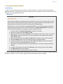
Page 4
Geocap plugins
Page 5
B. Geocap Interface (Shelf)
Introduction
Geocap has a very customable interface. The user may even program a new interface and develop new
functionality. The concept of commands and schemas are key elements of understanding and operating
Geocap.
Exercises
Geocap project
Geocap is operated through projects. The project "holds" the data in a folder-like structure, similar to Windows
"File Explorer". All datasets are "children" of either a folder or another dataset. Geocap offers different project
templates, giving you a pre-defined folder structure that fits your workflow for a specific type of work.
Exercise
Open the Atlantis project
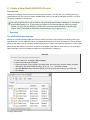
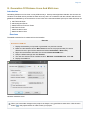
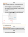
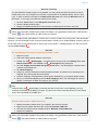
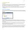
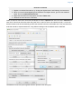
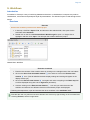
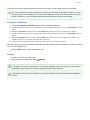
1. Click File > Open > Project and browse to the location of the Atlantis project.
2. Select the Atlantis.db file and click Open. A window similar to the one below will appear.
An open project
Tip
Next time you can open the project by using File > Recent Projects.
Pressing the small triangles (or '+' in older Windows versions) to the left of a folder will display the folder's
contents. Datasets and folders are organized very similarly to a file tree structure. A folder can contain other
folders, or datasets.
Note that there are two "modes" of the project view. Switch between these two by clicking on the tabs; Li
st and Tree. List view sorts folder content into a separate window, while Tree view sorts everything into
the tree itself..
Page 6
Exercise
Explore the project folder structure
Navigate through the folder structure taking notice of how folders and datasets are organized.
Datasets and folders can be cut, copied, pasted, renamed and deleted. This is performed from the
popup menu which appears when right-clicking a dataset.
1. Expand the folders and observe the subfolders
2. Look at the right-click menus.
On folders, the Multiple will allow multiple folders to be selected for cutting, copying or deleting. The
right click popup menu also contains commands which may be executed on the datasets. Notice the
different icons of the different datasets. They correspond to the schema of the data set. The name of
the schema is written in the second column.
Display data
Exercise
Display data
Display the various datasets in the project
1. Locate a grid dataset (structured points or seabed) e.g. 2. Seabed/Grids/atlantis
2. Right click the dataset and try a display command e.g.
Display, Map Data, Map sea or Ma
p land.
3. Right click the dataset again and select Zoom to Data. This will make the display window
center the graphics window around the dataset.
4. Display some of the lines e.g. lines found under 1. Maritime Lines by right-clicking and
selecting the command
Display
5. Check, and uncheck the checkboxes to the left of the displayed items and observe that this
toggles displayed objects on/off. You can also check and uncheck the folders containing
displayed items.
6. Items can also be displayed double clicking on one of the commands in the Toolbox (Item,
Schema and Shared commands)
Note how the displayed items are shown and hidden from the display window.
Note that by checking and unchecking the first level folder 1. Maritime Lines, or 2. Seabed all datasets
displayed under this folder are shown and hidden.
Page 7
Visualizations are called actors
Exercise
Commands: In panel Help
1. Open the command called "Generate 200M Line" from the toolbox.
2. Click the icon with the
question mark to open the in-panel help.
3. Read the information that pops up.
Navigating the graphics window
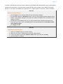
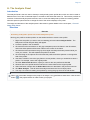
Note: Operating Geocap with a two-button mouse or using the Touch-pad is possible but not
recommended. The recommendation is a three-button mouse with a wheel, see picture below.
You may use the computer mouse to move around in the display window. You do this by pressing one of the
mouse buttons while the cursor is in the display window, and moving the mouse while keeping the button
pressed.
Rotate - Left mouse button
Pan - Middle mouse button (or wheel) or Shift + left mouse button
Zoom - Right mouse button
Scale Z - Mouse wheel (scroll)
Spin - Ctrl + left mouse button
The mouse buttons
Page 8
Scrolling the mouse wheel is one way to scale depth values of the dataset. The z values can also be
scaled by clicking the Actor Scale
button in the toolbar and dragging the z slider.
Tip
Set the focal point by positioning the mouse cursor on a desired point in the display window and push
the X key on the keyboard. This focal point will be the center of the display and the point of rotation.
Exercise
Navigate using the mouse and navigator panel
1. Use the mouse in the display window to zoom, pan, and rotate the data view in the
graphics window. Instead of using the mouse for navigation, you may also use the Naviga
tor
2. Click the
button in the main tool bar and the navigator panel should appear.
3. Try the different buttons in the navigator.
Important Toolbar Buttons
Basic Concepts in Geocap
The interface to the UNCLOS specific features in Geocap are through the use of schemas on datasets and com
mands. The commands can be found in the Toolbox to the right in the Geocap interface or at the top of the
menu which appear when you right click a dataset. Which commands are displayed in the right click menu
depend on the schema of the dataset. A Base Line will contain commands appropriate for the Base Line schem
a, while a Bathymetric Profile will contain different commands.
Schemas
Geocap uses schemas to classify a dataset. The Shelf Module contains several schemas. Some of the schemas
used in the Shelf Module are coast line, base line, limit line, seabed, sediment thickness. You can define
the schema of a dataset in the project by right clicking it, and selecting set schema in the pop-up menu. The
choice of a dataset´s schema controls which commands you see in the pop-up menu when you right click the
dataset. You may create your own schemas as well as edit existing schemas by selecting schemas under edit
in the main menu. You can also edit the commands associated with the schemas.
Commands
Commands are operations which can be performed on a dataset. Commands can for example be used to
display a dataset in the display window, or to generate new datasets. You can even create your own scripted
commands to cater to your specific needs. You execute a command by right clicking the dataset or folder you
want to run it on, and then selecting the relevant command in the pop-up menu. You can give different
parameters to a command in the command editor. These parameters are stored with the command and used
during execution.
Commands can be stored in three categories:
1. Item commands
2. Schema commands
3.
Page 9
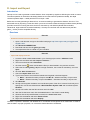
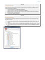
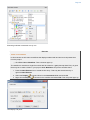
3. Shared commands.
You will find the commands sorted into the different categories in the Toolbox (see illustration below) or on the
right-click menu of a dataset or a folder. Commands are also put together in sequence in Workflows to perform
visualizations or data operations, see chapter S.
All commands have a front end panel, and most of them have settings that may be customized.
An example of a command front end panel
Item Commands
A command can be stored at the level of a dataset or a folder. This is called an item command. This command is
unique to this dataset or folder, it "belongs" to that dataset. You can see these commands on the top of the Tool
box or in a sub menu when you right-click a dataset and select Item commands. Most items in the project do
not contain any item commands by default.
Exercise
Create an item command
1.
2.
3.
4.
Go to 1. Maritime lines / 60M lines and select one of the datasets.
In the Toolbox right click Display.
Set Line Width to 4.
Check User defined Color and set the color to white.
5. Click the
icon in the upper right corner of the menu and observe that the command
appears in the Toolbox under Item Commands.
6. Click Cancel (the settings will not be saved for the schema command).
7. Right click the Display command under Item Commands and select Rename.
8. Rename it to Display in white and click OK.
9. Select the different lines in 1. Maritime lines / 60M lines and observe that the new Display in
white command is only available for the one dataset.
Schema Commands
A command stored at a schema level is called a schema command. All datasets or folders using the same
schema share these commands, which also means that editing these commands will affect all the datasets using
this schema. The schema commands of a dataset are listed on the top of the right-click menu.
Page 10
The Geocap Toolbox. Note that the_ *{_}Filter{_}* _is checked, meaning that commands not specifically relevant
are invisible. Untick the filter to show all commands.
Exercise
Get familiar with schema commands
Right click the different datasets in the project, and see how the right click menu changes from
schema to schema.
Default command
The default command is the command that is executed when you tick the box next to a dataset in the project.
By default a dataset will have one of the schema commands as a default command. This can however be
changed.
Exercise
Change the default display for seabed surfaces
The seabed surfaces has a default command "Map sea" or something similar.
1. Click on the Seabed datasets in the 2.Seabed / Grids folder.
2. In the Toolbox right-click another command (i.e LOD Grid Display) and select Set as default
command
3. Tick the checkbox next to the Seabed dataset and notice that the new command is executed.
Shared Commands
Shared Commands are commands which are shared with all datasets and folders. The shared commands are
listed in the Toolbox under Shared commands. If you cannot see the Toolbox, it can be opened from View on
the main menu.
Page 11
All commands have a command editor where you may change the properties, thus affecting the way it is
executed.
Exercise
Create a new command for custom display of limit lines.
1. Click on one of the datasets with the limit line schema inside the 1. Maritime lines folder
2. Right click the Display command under Schema commands in the Toolbox and select Copy
3. Right click Schema commands in the Toolbox, select Paste and observe that a copy of the
selected command called Display-1 will appear in the schema command list.
4. Right click the new command in the command list, and select Rename
5. Name the command Display Thick Yellow
6. Right click the command and select Edit. The command editor for the selected command will
appear
7. Set Line width to 6
8. Check the User defined color box and click the Palette button.
9. Select a yellow color and click OK
10. Click OK to close the Display command editor
11. Right click the same data set, and observe that our new command is present in the right click
menu. This is because the Pin to Menu check box next to the Display Thick Yellow comman
d in the Toolbox is checked.
12. Un-check the Pin to Menu check box next to the Display Thick Yellow command in the Tool
box.
13. Right click the same data set again, and observe that our new command is not present in the
right click menu.
14. Execute the command by double clicking Display Thick Yellow in the Toolbox. Observe that
the line is displayed in yellow.
15. Check the Pin to Menu check box next to the Display Thick Yellow command in the Toolbo
x again. Now right click a different dataset with the same schema (limit line) and observe that
the new command can be executed on this right click menu as well.
Tip
The Pin to Menu check box lets you decide which commands should be available in the right click
menu, so it is easy to keep organized. Try to experiment with this option to manipulate the right click
menu.
The Sticky Surface
Geocap has a concept where any surface can be set to be sticky. When a surface is sticky, data like points,
lines or images may be displayed onto that surface. This is mainly done by re-sampling lines and displaying
them a little bit above the sticky surface.
When a surface is activated (or set) as a sticky surface, it is copied to workspace (visualized in the toolbox)
under the name sticky_surface. If this dataset is removed from workspace, there is no sticky surface anymore.
Page 12
Exercise
Display onto the Sticky Surface
1. Right-click on a Seabed surface dataset and select
Set as sticky surface
2. Select a line, e.g. Atlantis > 1. Maritime lines > 200M lines > atlantis + 200M in your project.
3. In the Toolbox under Commands > Schema commands right-click and Edit on the
Displ
ay command.
4. Check the Glue to Sticky Surface and press Execute to do a line display.
5. Uncheck the Glue to Sticky Surface and press Execute again and observe the difference.
Warning
Note that points and lines displayed onto a sticky surface are displayed without their original z-values,
and this may not be what you intend to do when displaying a foot of slope point or a bathymetric line.
Keep that in mind.
Keyboard shortcuts
Geocap has several keyboard shortcuts or hotkeys. Go Help > Keyboard shortcuts to bring up a list.
A selection of the most important keyboard shortcuts:
Key
Explanation
Key
Explanation
o
Toggle color code for last used map command
on/off.
+
Zoom in.
s
Turn graphics into surface mode.
-
Zoom out.
v
Value of height/depth (z coordinate) from
graphics.
2
Toggle graphics to 2d mode.
w
Turn graphics into wire mode.
3
Toggle graphics to 3d mode.
x
Setting the focal point. The graphics will rotate
around this point.
3
Toggle stereo view on/off when stereo is
activated.
y
Cursor point is set at the surface of the graphical
element.
z
Zoom by drawing a rubber band with left
button on the mouse.
j
Snap to any point on a displayed line.
When using j or y to snap to lines or surfaces, Geocap will report what you have snapped to in the lower
left corner.
Exercise
Keyboard shortcuts
Visualize a seabed surface and test all the above mentioned keyboard shortcuts.
Page 13
C. Create a New Shelf (UNCLOS) Project
Introduction
Geocap provide empty folder structure for various types of projects. This will give you a starting point to get
organized with your own project. A project template either gives you a ready made folder structure, or it gives
you a suite of folders to choose from.
An empty project structure may be used for communicating relevant data to colleagues, or for analysis
and trouble shooting by us. To send parts of a project to us in Geocap Support, even only a single
dataset, you may copy the dataset (or a folder) from your main project and paste it into this empty
project. Then zip and send the disk folder projectname.zip to [email protected].
Exercises
The UNCLOS Project template
Geocap can provide an empty folder structure for UNCLOS projects. This will give you a starting point to get
organized with your own UNCLOS project. The default folder structure holds empty folders for most of the data
types you will need. If you do not find a suitable folder you can create a new folder for that data. It is also a good
idea to create sub-folders if you have a lot of data, for example a sub-folder for each survey or for each region.
Other subfolders commonly created are folders for FOS Collections, Images etc.
Exercise
Generate a new and empty UNCLOS project
In the main menu, click File > New > Project
Select UNCLOS project template
Type in the name of your project in the Name field. The name may consist of letters, numbers
and spaces, but special characters like [, æ,ø, å, &, /, % ... should be avoided.
Click the Browse button, and select where you want to store your project on your hard disk.
Click Finish
An empty Shelf project
Page 14
The idea is that this basic structure is kept. Folders may be added and data imported, but the original folders
should not be renamed or moved, and their schemas should not be changed. This is because this folder
structure is used when new datasets are generated. If an original folder is not present, it will be recreated.
Exercise
Explore the project settings
Click the
icon on the project toolbar to look at the project settings.
Pay particular attention to Geodetics section. Here you may activate geodetic settings for the
project. If the geodetic settings for the project are checked, all data will be converted to these
settings on import.
Set Geocap to automatically zoom to your project area when the project is opened by first
zooming to your area. Then in the Data section click Use current and tick Set data window
when loading project
Click Apply and OK
Exercise
Copy data into your new project
1.
2.
3.
4.
Open your Atlantis project (or another project)
Right-click and copy a Seabed surface from the Atlantis project.
In your new project, go to the 2. Seabed / Grids folder, right-click and do Paste
Do the same for a coastline.
Page 15
D. Import and Export
Introduction
Geocap can be used to generate accurate distance lines computed by algorithms following the earth curvature.
The same operation is used when calculating distances from the base line (200M and 350M), the depth
constraint (2500m depth + 100M) and the Foot of slope + 60M.
Before we can start generating a distance line, we need something to generate the distance line from. This
tutorial will start by importing a coast line within your area of interest. National Geophysical Data Center (NGDC)
provides coast lines covering the entire world in a data set they call GSHHS (Global Self-consistent,
Hierarchical, High-resolution Shoreline Database). Geocap can read both the raw data format (the files
gshhs_*.b files), and the shapefiles directly.
Exercises
Exercise
Download coastline files from the Internet.
1. Open a web browser and go to this NGDC web page: http://www.ngdc.noaa.gov/mgg/shorelin
es/gshhs.html.
2. Click Download GSHHS Data.
3. Download and save the file gshhs_2.2.2.zip.
4. Uncompress the files to a folder on your hard disk.
Exercise
Import and display coast line
1. Locate the folder called Coast Lines in your Geocap project under 1. Maritime Lines.
2. Right click the folder and select Import > Generic….
3. The format should be set to Automatic.
4. Click the browse
button and locate the files you downloaded in the previous exercise.
5. Select the file called gshhs_h.b (this is a high resolution, but not the full resolution), and click
Open.
6. Click the Area of Interest tab.
7. Check the Import Area check box.
8. Type in the minimum and maximum latitude and longitude in decimal degrees.
a. Max Y = Northern boundary of import area Min X = Western boundary of import area
b. Max X = Eastern boundary of import area Min Y = Southern boundary of import area
9. Click Execute.
10. Geocap will recognize the datum and coordinate system of the file. If it doesn't it will ask you to
specify this. In that case select datum: World Geodetic System 1984 and coordinate system:
Geodetic.
11. Geocap will confirm that the file has been read. Click OK.
12. After the file has been read, click the Cancel button in the Generic reader dialog.
13. Observe that the imported dataset is stored in the Coast lines folder.
14. Right click the dataset and select Zoom to Data
15. Right click the dataset and select Display
The data is imported in Geodetic, with latitudes as Y coordinates and longitudes as X coordinates. In order to
view the data in a proper projection, we convert the data to Mercator coordinates.
Page 16
Exercise
Convert coast line to the right projection and display
1.
2.
3.
4.
5.
Click the dataset and go to the Shared commands section in the Toolbox.
Double click the Convert to Mercator... command in the Operations folder.
Change the result combo box to Replace input.
Click Execute.
Agree to replace the existing dataset by clicking Yes.
The data is now converted. Let us re-display in new coordinate system:
1. Right click the dataset and select Zoom to Data
2. Right click the dataset and select Display
If you have a data set with the base line of your country you can import it and use that as a base for the distance
lines. If you do not have such a base line, skip this exercise and generate a false base line in the next exercise
instead.
Exercise
Import Base line ASCII lat-lon format
1. Locate the folder called Base Lines in your Geocap project under 1. Maritime Lines
2. Right click the folder and select Import > ASCII Column… and the ASCII Column import
dialog will appear. (You can make dialog bigger by clicking in one of the corners and drag.)
3. Click the browse
button and select your base line file. There may be a suitable file
somewhere under Atlantis/Data/...
4. Adjust the number of header lines in your file with the Adjust header spin box. The header
lines should be displayed in the top part of the file preview, while the bottom part of the file
preview should hold the coordinates.
5. If the columns are delimited by space or tab characters, you should keep the column separator
at white space. If the file uses a special character, change the combo box to MySeparator,
and change the value by typing in the separator directly in the combo box.
6. Select a coordinate format:
a. Deg = decimal degrees
b. Deg min = degrees and decimal minutes
c. Deg min sec = degrees, minutes and decimal seconds
d. Hemi = hemisphere (N/S for north or south, E/W for east or west)
7. Set the correct file columns for each data column. You see the first lines in the table. On top
of each table is a spin box with the file column number. Adjust the file column by clicking the
spin boxes so that the file columns are interpreted correctly.
8. All other parameters should be OK with the default settings, click Execute.
9. The file has now been imported. Click the Cancel button in order to close the ASCII Column
import dialog.
Page 17
Exercise Continued
Convert Base line to Mercator and display
The data is imported in Geodetic, with latitudes as Y coordinates and longitudes as X coordinates. In
order to view the data with the coast line, we convert the data to Mercator coordinates.
1.
2.
3.
4.
5.
Click the dataset and go to the Shared commands section in the Toolbox.
Double click the Convert to Mercator... command in the Operations folder.
Change the result combo box to Replace input.
Click Execute.
Agree to replace the existing dataset by clicking Yes.
The data is now converted. Let us display the data:
1. Right click the dataset and select Zoom to Data
2. Right click the dataset and select Display
Note that the conversion is not needed if the Project Projection is activated under Project settings.
Exercise
Open the base line in table view
1. Select some points in the table view and observe that points selected in the table view are
highlighted (in yellow) in the display.
2. Observe that you can copy entries from the table view and export to a text editor
3. Click Edit mode. Try to add an extra column and/or change names on the base line points.
Export
Exercise
Export the baseline
Export the baseline in Ascii column format as Degrees Minutes Second.
Page 18
E. Baseline Generation (Simplified)
Introduction
The baseline is needed in order to generate distance lines. The coast may also be used as a baseline (by
changing the schema accordingly), but then the computing time may be very long.
If you do not have a baseline for your area, you may generate a dummy to use as an approximation based on
the coast line you imported in a previous exercise. If you already have imported an official baseline you may
skip this exercise.
Exercises
Exercise
Generate dummy baseline
In this exercise we will use the digitizer to snap values from the coastline, in order to make a baselin
e.
1. Display the coast line called GSHHS, which should have been imported in 1. Maritime Lines /
Coast lines.
2. Open the Digitizer by selecting Tools > Quick digitizing from the main menu.
3. Check the option Save also in folder, and click the Browse button.
4. The project view dialog will appear. Select the Base lines folder under 1. Maritime Lines,
and click OK
5. Click Start digitizing
6. Digitize the points on the coast line by pressing j on the keyboard. The picks will automatically
snap to the nearest point on the coast line data set. Digitize a rough version of the coast line
by picking the outermost points on the coast line.
7. When you are finished digitizing click the Stop digitizing button. The digitized line should
appear in the Base lines folder.
8. Locate the digitized baseline in 1. Maritime lines / Base lines
9. Right click the dataset and select Rename. Rename the data set to your country name and N
o_dummy_baseline.
10. Right click the dataset (not the folder), and select Set Schema > Base line
Digitizing a baseline
An alternative is to use the command object
needed for a distance calculation.
Red snapper on the coast line and simply snap the outer points
Page 19
Exercise
Use the
"Red snapper" to generate an alternative baseline
1. Click the coast line called GSHHS.
2. Double click the
3.
4.
5.
6.
7.
8.
Red Snapper... command which can be found in the Editing folder under
Shared commands in the Toolbox. The
Red snapper dialog will appear.
Click the Display selected data with green points button. This will display the points that
the coastline is generated from.
Check the Save in project box and click the Browse button.
Select the Base lines folder and click OK.
Click Start snapping.
Start clicking on the outer points on the coastline with your left mouse button.
When you are finished digitizing click the End snapping button. The red snapper line should
appear in the Base lines folder.
Observe that in the
Red Snapper command (and also in the Tools > Quick Digitizer) you may
enhance functionality by enabling more keys. E.g. m can be used to snap all points up to next picked
point. This is probably not needed here.
Page 20
F. Bathymetric Grids And Generation Of Bathymetric Profiles
Introduction
The use of bathymetry is a very central element when working with the determination of the extension of the
continental shelf according to UNCLOS Article 76. It is relevant both for the depth constraint (2500m depth
+100M) and the determination of the foot of the continental slope. In Geocap, bathymetry can have several
different forms:
Singlebeam bathymetry may be imported as bathymetric profiles.
Multibeam bathymetry or other spread point data with depth measurements can also be imported. In
order to use the foot of slope analysis tool on point data, the dataset must be gridded first.
Grids may be imported directly into Geocap. Geocap supports import of several different file formats; the
most common and useful kind of bathymetric data is the ETOPO1 grid. The ETOPO1 Grid is provided by
NGDC (National Geophysical Data Center). This grid will not be accepted by the Commission as a basis
for your foot of slope points. However once you have imported the grid you will be able to see the shape
of the sea floor, and in particular the approximate position of the Foot of Slope or base of slope region.
Exercises
Exercise
Download the ETOPO1 grid from the Internet
1. Open a web browser, and go to the following address: http://www.ngdc.noaa.gov/mgg/global/g
lobal.html
2. Click the link: Extract Custom Grids - in the left column on the page, below the globe. A new
web page with a interactive map should appear.
3. Zoom into the area where you want to extract the grid.
4. Click the icon with and i in the upper left corner of the map window.
5. Drag a rectangle over the area where you want to extract the grid. You should see a red
rectangle on the map.
6. Keep Layer as ETOPO1 (ice)
7. Select Output Format XYZ
8. Click "click here to download"
The following exercise can be used on most binary grids which Geocap supports. You normally do not
have to specify the grid file format. Geocap will automatically recognize the file format.
Page 21
Exercise
Import the grid into a folder in your project
1. Locate the folder called Grids in your Geocap project under 2. Seabed
2. Right click the folder and select Import > Generic…
3. The format should be set to Automatic.
4. Click the browse
button and locate the file you downloaded in the previous exercise.
5. If Specify import area is checked, uncheck this option. This will import the entire grid.
6. Click on the Reader Options tab and under polydata and check the box next to Invert (The
Grid we will import has negative values for sea depths, and positive values for heights above
sea level. Usually bathymetry data has positive values for depths. We therefore have to
multiply the depth and height values by -1 with this option to "flip" the data).
7. Click Execute.
8. You will now be prompted with a question of the coordinate system and datum. Select: World
Geodetic system 1984, Geodetic and click OK.
9. Geocap will report if the grid has been imported correctly; click OK and close the import dialog
by clicking Cancel.
10. Observe that the new data set has appeared in the Grids folder.
Exercise
Convert the grid to Mercator coordinate system
The data is imported in Geodetic, with latitudes as Y coordinates and longitudes as X coordinates. In
order to view the grid with the data we have already imported and converted to a Mercator coordinate
system, we need to convert this grid to match the same coordinate system as the other data in the
project (Mercator).
1. Click the dataset and go to the Shared commands section in the Toolbox.
2. Double click the Convert to Mercator... command in the Operations folder. (or another
relevant datum / coordinate system)
3. Change the result combo box to Replace input.
4. Click Execute.
5. Agree to replace the existing dataset by clicking Yes.
6. Geocap will report if the grid has been converted correctly, click OK and close the conversion
dialog by clicking Cancel.
7. Check that the schema of the dataset is seabed surface. If not then right click the dataset,
choose Set Schema and choose seabed surface.
The data is now converted and ready to be displayed:
1. Right click the dataset and select Zoom to Data
2. Right click the dataset and select Map Sea
3. Right click the dataset and select Map Land
When you have made changes to the project it is always a very good idea to store them. Click the save
button
in the project tool bar in order to save your project.
Exercise
Crop out smaller grids from your Seabed surface
Use the command Crop to chop out 2-4 smaller grids from your main seabed surface.
Use keyboard shortcut z in 2d mode to set a window frame
Page 22
Exercise
Display a detailed contour pattern on the seabed surface
Use the command
General Display to display contours. Try to display line contours at depths
relevant to base of slope and see if you can observe the area of the deep ocean floor and areas of
base of slope from the contour pattern.
Explore the different display options of this command, and observe that this command is different
from most other commands. Observe that this command can produce several actors (visualizations).
Exercise
Generate a Bathymetric Profile from a grid
1. Locate the dataset you imported in the previous exercise, which should be located in 2.
Seabed / Grids. The data set should have the schema Seabed Surface. If it does not have
this schema, right click it and select Set Schema > Seabed Surface.
2. Display the seabed by right clicking it and selecting Map Sea.
3. Right click the dataset and select the command Display contours...
4. A menu will appear. We will just use the default settings. Click Execute, and Cancel.
5. Right click the dataset and select the command Generate Bathymetric Profile. A menu will
appear.
6. Click the Start button, then digitize the first point of the profile by clicking with the left mouse
button where you want the profile to start on the seafloor in the display window.
7. Digitize the last point of the bathymetric profile by clicking with the left mouse button where
you want the profile to stop on the seafloor.
8. After you have digitized both the start and stop point, you will be prompted with a dialog asking
you to provide a name for the profile. Keep the default name and click OK.
9. Geocap will notify you where the resulting Bathymetric profile has been stored in the project.
Click OK.
10. Locate the new profile in 2. Seabed / Bathymetric Profiles; this is the default position of
bathymetric profiles. In order to structure our project we want to move the profile into a sub
folder and rename the profile.
11. Right click the folder 2. Seabed / Bathymetric Profiles and select New > Folder.
12. Change the folder name to Etopo1 and click OK.
13. Right click the profile and select Cut.
14. Right click the new folder and select Paste. The profile is now moved into the new folder.
15. Right click the data set and select Rename. Give the profile a suitable name, for example the
name of the area you are working in.
Page 23
G. Generation Of Distance Lines And Mid-Lines
Introduction
Calculating distances can be done in many different ways. Geocap uses algorithms that take into account the
curvature of the Earth which provides for better accuracy and is in accordance with the scientific and technical
guidelines established by the Commission on the Limits of the Continental Shelf (CLCS) for UNCLOS Article 76.
12M Territorial Seas.
24M Contiguous Zones.
200M Exclusive Economic Zones
60M Formula Lines.
100M Constraint Lines.
350M Constraint Lines.
Exercises
The 200M constraint line is measured from the baseline.
Exercise
Generate the 200M line
1. Display the baseline you imported or generated in a previous exercise.
2. Make sure the baseline has the Base Lines schema in the project window (If it uses a
different schema, right click the dataset and select Set Schema > Base Line).
3. Right-click the baseline and select the command Generate 200M Line....
4. Keep the default settings and click Execute.
5. The new line should now be available under 1. Maritime Lines/200M Lines. Click OK.
6. Display the 200M line.
Generate 200M line menu
When you have made changes to the project it is always a very good idea to store them. Click the save
button
in the project tool bar in order to save your project.
Page 24
Exercise
Read about distance lines in the
in panel help
1. Open the command Generate 200M Line... from the toolbox.
2. Click the icon with the
question mark to open the in-panel help.
3. Read the information that pops up. If you want to use the method of tracés parallèles you
may consider resampling (geodetically correct) your baselines and use distance from points.
Exercise
Check Table View for the 200M line
1. Right click the 200M line and select Table View.
2. Observe the columns, Base Line, Base Line Index and Second Base Line Index. This tells
you which baseline and which point on the baseline that contributed to the point on the 200M
line.
3. Scroll down to a point that has values in both Base Line Index and Second Base Line Index
and highlight this point
4. Observe that this is the crossing points between two arcs in an envelope of arcs calculation
(equidistance point). That is why it is referring to two basepoints.
Exercise
Generate new 200M line with 0.5M point spacing and baseline critical points
1. Select the baseline dataset in your project.
2. In the Toolbox, right-click Generate 200M line... and select Edit.
3. Type in the new point spacing 0.5 and tick the checkbox that says Generate base point
connection polygon
4. Click Execute and OK
5. Note that the line will have Connection Polygon at the end of its name.
You have now set the Generate 200M Line to use 0.5M point spacing on the distance line. Note that if you
reduce the point spacing the algorithm needs more time to do the calculation.
Exercise
Display base point connection polygon
Notice that not all points on the baseline are included as critical points used to generate the 200M li
ne. This is helpful in determining and visualizing which points on the baseline contribute to the limit
lines, whether the user generates 200M, 24M, 12M or any other distance calculation with this option.
1. Right-click the baseline dataset and click Display Points
2. Now right-click the 200M line with Connection Polygon at the end of the name, and click Displ
ay. Also display the points by right clicking and choosing Display Points.
3. Notice how the polygons points back to the critical points on your baseline (see image
below).
4. Toggle the display between polygon mode and wire mode with the W and S keys.
Page 25
200M line with critical points on baseline in blue
Exercise
Generate 350M line
The same procedure as above.
Exercise
Try the Distance Calculation tool
Use the Distance Calculations tool to verify that the distance between the baseline and the
generated 200M line is correct.
1. Open the tool from Tools > Distance Calculations.
2. Select an appropriate datum and coordinate system.
3. For distance calculation method, select Vincenty calculation. Flat earth calculates in the
metric values of the projections.
4. To measure the distance between two points, press j on the keyboard to snap to them.
5. The distance is displayed in the lower part of the panel. Notice that vertical, horizontal and
total distance is measured and that lat/long of the select point is listed.
Exercise
Clean up the distance lines
Remove the parts of the generated distance lines that are outside our area of interest.
1.
2.
3.
4.
Right-click on the dataset and select Edit points and lines...
Click on the Delete tab, then on the By closed line tab.
You may want to redisplay your data using the Display button in the lower part of the panel.
Click the Start button and start digitizing, encircling the parts of the lines that should be
removed.
5. When encircling is almost complete, click the Connect to start and End button. Then press D
elete points INSIDE to remove the encircled points. (Alternatively use OUTSIDE).
6. The edited dataset is not written back into the project until Execute is clicked. Observe the
options for Save as an extra copy, Overwrite input dataset etc.
Page 26
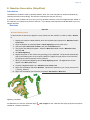
Exercise
Generate mid-lines
Generate mid-lines between The Kingdom of Atlantis, the Republic of Starfish Islands and The
Federate States of Five Stone Islands
1. Display the three baselines in the project.
2. Right-click one of the baselines in the project and select Generate midline...
3. Tick the radio button Specify: and click Rubberband select (the window will be set to 2D
mode).
4. Drag a rectangle around the area where you want the midline to be created. Notice that the
coordinates are updated accordingly in the menu (see image below).
5. Keep the default values of the other settings.
6. Click Execute
7. In the window that pops up, clik OK. If you only wanted to calculate against one country, you
could have selected only that country in this menu.
8. Locate the midline in 1. Maritime lines / Mid lines and display it. Display the points also.
Generating a midline. Note that is is generated within the window frame (shown in black).
It is also possible to generate base point connection polygons to extract critical base points, the same
way as with distance line generation.
Exercise
Mid-lines using weighted base points
Try to add weights on base points and see what happens to your mid-line. Read the In-Panel Help in
the Generate midline command to understand how to use weight on base points.
Exercise
Check Table View for the midline
1. Right click the midline and select Table View.
2. Observe the different columns in the Table View,
Page 27
H. The Analysis Panel
Introduction
The Analysis Panel is the tool used in Geocap to analyze bathymetric profile data, which can then be used to
determine the Foot of the Continental Slope in accordance with UNCLOS Article 76. This section provides an
overview of what the analysis panel looks like, how to create new bathymetric profiles from existing profiles
when this panel is open and how to change the look of the various displays in the panel.
The usage and elements of the analysis panel is discussed in greater details in the next chapter, I. Foot Of
Slope (FOS) Points.
Exercises
Exercise
Generating a bathymetric profile from another bathymetric profile
Moving your profile to another position on the seabed surface to create a new profile.
1. Right click the profile you want to use as a starting point and select Analyze Profile. The
Bathymetric Profile analysis dialog will appear.
2. Locate the profile in the 3D window.
3. Click with the left mouse button on the gray transparent part of the frame in the 3D window,
and some white spheres will become visible in the corners of the frame.
4. Click with the left mouse button the gray frame again and keep the button pressed while you
move your mouse. This will translate the profile to the side.
5. Click and drag on the spheres This will rotate the profile around the spheres on the opposite
side of the profile.
6. Use these controls to move the gray frame to a new position, where you would like to store a
profile. For example, next to the original profile.
7. Click the Save Profile As button, specify a name for the new profile and click OK.
8. Observe that a new profile has been stored in the same folder as the original profile.
9. Select the Base of Slope with the Select Area button as described in the previous exercise.
10. Click New Analysis. This will store the analysis and store the Foot of Slope points.
11. You may now continue creating new profiles by moving the gray frame in the 3D window.
When you have made changes to the project it is always a very good idea to store them. Click the save
button
in the project tool bar in order to save your project.
Page 28
I. Foot Of Slope (FOS) Points
Introduction
The Analysis Panel is one of the most important tools in Geocap because it allows you to determine the Foot of
the Continental Slope in accordance with UNCLOS Article 76. FOS analysis is crucial because both formula
lines (Gardiner and Hedberg) are calculated using FOS positions.
The elements of the FOS analysis panel
Some of the key variables that can be adjusted in calculating the change in gradient are:
Change of average gradient.
Change of gradient.
Gradient.
Average gradient.
Some of the other key features are:
Select area (base of slope zone)
Clear area
Flip Profile Direction
Save Profile As...
Save Analysis As...
Calculation interval
Browse crossing lines or grids from the project
Depth scale
Various Filters for smoothing noisy data or complicated morphology
Exercises
Page 29
Exercise
Calculating the Foot of Slope (FOS)
Use the analysis panel to set foot of slope points.
1. Right click the profile you generated in the previous exercise.
2. Select the command object called Analyze Profile.
The profile analysis tool will appear at the bottom of your screen. You may need to un-dock
the panel or expand it by dragging the edge of the window up, allowing more space to view it
properly.
The black line with gray dots is the seafloor, the red dotted line is the change of gradient and
the thicker red vertical line marks the point of the maximum change of gradient on your profile.
The same profile is also visible in the 3D window above the analysis panel where you will
notice the red vertical line marking the maximum change of gradient.
3. If you want to flip the direction of the profile in the 2D window, you may do so with the flip
profile direction button.
4. Click the select area button.
5. Click with the left mouse button in the profile window, and keep the left button pressed. Drag
the mouse to the side, and release the button. This is how you select the area where the
software will calculate the change of gradient.
If you do not use evidence to the contrary, the foot of the continental slope should be placed
at maximum change of gradient at the base of the slope. So we want to restrict the calculation
of the change of gradient to the base of the slope. Determining the Base of the Slope may
be quite complicated, and is subject to individual interpretation, therefore we will not go into
details about determining the base of slope zone in this tutorial. For more information refer to
the Scientific and Technical Guidelines of the Commission on the Limits of the Continental
Shelf found here: http://www.un.org/Depts/los/clcs_new/commission_guidelines.htm
6. Click the select area button again and select the part of the profile which you want to use as
the base of the slope.
You may change the parameters of the algorithm several times but for this exercise we will
keep the default settings.
7. Click the Save Analysis as.. button. You will be asked for an analysis name and a foot of
slope point name.
8. Click the plus sign (or triangle) next to the profile in the project manager and you will see that
the FOS analysis is stored as a child of the profile in the tree.
9. Click the plus sign (or triangle) next to the FOS analysis dataset, and you will see the Foot of
Slope dataset. This is the data set holding the foot of slope point we just made.
10. Click the Exit button in the bathymetric profile Dialog in order to close it.
The area selected by the Select area button should possibly equal the Base of slope (BOS) area. If you
have a BOS-outline polygon, then browse it into your analysis.
Info
Whether you see a plus sign or a triangle in the project manager is determined by your Windows
operating system or settings. The default for Windows XP is a plus sign and the default for Windows 7
is a triangle.
Page 30
Exercise
Change the settings of the Analysis panel
Change the colors and other settings of the lines in the panel
1.
2.
3.
4.
Double-click the Seafloor entry in the right part of the panel.
Change line width and color.
Observe that the settings are remembered by Geocap.
Change the settings in the way that you want to use for all your FOS analysis documentation
in the future.
5. Press the Screen Shot button to write an image of the analysis to your project for
documentation. Alternatively, you may use the standard Print Screen windows option to
produce a picture to the Windows clip-board.
Exercise
Joining FOS points into one FOS group dataset
It is often useful to work with a group of FOS points instead of working with them individually. This
exercise will show you how to collect many FOS points into one foot of slope dataset. A foot of slope
point is stored as a dataset under an analysis which again is stored under a profile.
1. Click the small plus signs (or triangles) to the left of the profiles and the analysis datasets
2.
3.
4.
5.
6.
7.
8.
9.
10.
11.
12.
made in the previous exercise to show the foot of slope datasets.
Right click the first foot of slope point and select the command, set as active foot of slope.
Right click the next foot of slope point and select the command, Append to active foot of
slope.
Repeat the last step as many times as necessary to append all the foot of slope points you
want in one collection.
Right click the folder 2. Seabed and select New > Folder. The New Folder dialog will appear.
Select the Generic type (which is default choice).
Select the name to be Foot Of Slope.
Click OK.
Right click the new folder (Foot of slope) and select New > Workspace data > fos.
The Foot of Slope collection is now added to the folder.
Right click the new dataset and select Set Schema > Foot of Slope.
Right click the same dataset again and select Rename.
Give the foot of slope a proper name, for example the area you are working in.
Exercise
Merge all FOS points into one datasets
This is an alternative to the exercise above. Instead of grabbing point by point, the FOS points can be
merged into one group by running a ccommand that has a filter.
1. Find the command Merge all FOS points on a bathymetric profiles folder.
2. Try it.
3. Check the filter settings for that command to understand how it works.
Exercise
FOS table view
Open the Table view of a FOS group. Look at the various field data.
Page 31
Exercise
Adding 60M to the FOS points
1.
2.
3.
4.
Display the FOS points which you created in the previous exercise.
Right-click the dataset and select the command object Generate 60M Line.
The new line should now be available under 1. Maritime Lines/60M Lines.
Display the 60M line.
Exercise
FOS+60M table view
Open the Table view of a 60M distance line. Look at the various field data and compare to the field
data of the FOS-points
It is possible to show crossing lines in the analysis window. Click the browse icon to the right in the
analysis panel and browse for a line the crosses the profile.
When you have made changes to the project it is always a very good idea to store them. Click the save
button
in the project tool bar in order to save your project.
It is possible to filter (e.g. smooth) the bathymetry and then click the Tables of values button. The
filtered result (i. e. the smoothed bathymetry) is then available in a tab, and may be extracted as a
project dataset.
Exercise
Smoothen the bathymetry
It is possible to filter (e.g. smooth) the bathymetry and create a new dataset.
1.
2.
3.
4.
You may use one of the Atlantis singlebeam datasets for this
Open the analysis panel
Set a filter e.g. Gliding Average
Double-click the 1. Filter in the lower left corner and change the settings of the line to be a
thick, orange line.
5. Observe the smoothed filtered seabed
6. Click the Tables of values button. The filtered result (i. e. the smoothed bathymetry) is then
available in a tab
7. Select all points (Click in the upper left corner) and then right-click inside the table and select E
xtract points.to create a new project data set.
Page 32
J. Real Bathymetric Profiles
Introduction
Real bathymetric profiles are measured, usually by sonar. They are not generated by extracting values from a
seabed grid or from any other data derived mainly from satellite altimetry, such as ETOPO1. An example of real
bathymetry is "Corrected Depth Bathymetry" from the U.S. National Oceanic and Atmospheric Administration's
(NOAA) Geophysical Data System (GEODAS).
To locate a specific line amongst hundreds of lines in a folder, display them all, then click at the icon
Locate project object from graphics, then point at the relevant line. This action will select your line in
the project.
Exercises
The GEODAS bathymetric profiles can sometimes be very long, covering areas that you are not interested in. It
is possible to adjust the length of the profiles in Geocap, so that you will only analyse the part you need.
Exercise
Save an adjusted bathymetric profile as a new bathymetric profile
1. Right-click a real bathymetric profile (not one created from a seabed surface) and select Analy
ze.
2. Find the white spheres at the end of the profile in the 3D view and adjust them by dragging the
spheres to the desired position.
3. In the bottom left corner of the Analysis panel click on Save profile As...
4. Specify a new name for the adjusted bathymetric profile and click OK > OK. The new profile
will be saved in the same folder as the original.
5. Right-click the new bathymetric profile and choose Analyze Profile. Notice the new
bathymetric profile is now a sub-set of the original profile.
Tip
In some instances the white spheres may be very small when the analysis panel is first opened. It may
be necessary to zoom in closer to find one of the ends of the profile. Once the white sphere is clicked on
once, the white spheres on both ends will become larger and easier to see when dragging them to the
desired position.
Exercise
Combine portions of two or more bathymetric profiles into a new bathymetric profile
1. Combine two or more datasets into one dataset. (The command Append all lines in folder m
ay be used.)
2. Use the command
bathymetric profile.
Red Snapper with the m option to sample points to your new
Note that it may be even easier to flip the folder schema temporarily to Outer limit and use the Outer
limit digitizer to combine bits and pieces of bathymetric profiles.
Page 33
K. The 2500m Isobath
Introduction
Computing the 2500m isobaths is necessary in order to determine the Depth constraint in UNCLOS Article 76,
which is the 2500m isobaths plus 100 nautical miles. The 2500m isobaths can be generated based on
bathymetry grids or on bathymetric profiles (from single beam bathymetry). The only ones that can be used for
an actual submission to the CLCS are 2500m isobath points generated from real bathymetry data. For a grid,
the resulting 2500m isobath will be a contour line. A bathymetric profile will produce one or more points
wherever the profile value is 2500m.
Exercises
Exercise
Generate the 2500m isobath from a Seabed Surface
1. Locate the etopo1 dataset which is located in 2. Seabed / Grids. The dataset should have the
schema Seabed Surface. If it does not have this schema, right click it and select Set schema
> Seabed Surface.
2. Right click the dataset and select Display 2500m isobath. Black lines will appear where the
2500m isobaths are located. You may notice that the isobaths cover a larger area than you
are interested in so we will restrict the area where the isobath is calculated.
3. Set the display window to 2D mode by clicking the 2D View button.
or typing 2 on the
keyboard.
4. Zoom the display window so that it only covers the area you are interested in.
5. Right click the seabed surface and use the command, Generate 2500m Isobath. This will
use the full resolution of the grid and calculate the 2500 isobath only in the area we are
focused on. If the display window is in 3D mode it will create the isobaths for the entire
dataset. If it is in 2D mode it will only create the isobaths inside the display window.
6. Locate the result dataset which should be in 2. Seabed / 2500 Isobath. The Isobath dataset
you have created may still have some line pieces which you want to remove before generating
the 100M line, for instance the pieces that are seaward of the FOS points.
Exercise
Edit the generated 2500m isobath
1. Clear the display window by clicking the
button in the main toolbar.
2. Right click the dataset and select the command Edit points and lines.
3. Click the Display button near the bottom of the Edit points and lines dialogue box in order to
see the isobaths.
4. Select the Delete tab.
5. Inside the Delete tab, select By closed line.
6. Click the start button, then digitize a closed polygon around the part you want to delete by
clicking with the left mouse button.
7. Click Connect to Start and End in order to connect the last digitized point with the start point,
and end the digitizing.
8. Click Delete points INSIDE.
Page 34
Exercise continued
The part inside the closed polygon is now deleted. You may repeat the three last points in order to
delete some more. The changes you make are not performed on the dataset directly, but as a local
copy. In order to store the changes in the Edit points and lines menu, click the Execute button at
the bottom. A new copy of the data set is stored in the folder.
1. Click the Cancel button in the Edit points and Lines menu.
2. Clear the display window again.
3. Display the edited isobaths and confirm that the unwanted parts have been removed.
When you have made changes to the project it is always a very good idea to store them. Click the save
button
in the project tool bar in order to save your project.
Ordinarily, a 2500m isobath generated on a surface (as a contour) contains very many points, often thousands
of points. It is recommended to snap a subset of these data to create a much smaller dataset containing fifty to a
few hundred more or less critical points to use as input for the 2500m + 100M generation. For this we use the
command Red Snapper
.
Exercise
Use the Red Snapper to prepare for generating the 2500m + 100M
1. Blank the screen
2. Select the 2500m isobath dataset in the project.
3. Double click the
4.
5.
6.
7.
8.
Red Snapper... command which can be found in the Editing folder under
Shared commands in the Toolbox. The
Red snapper dialog will appear.
Click the Display selected data with green points button. This will display the points that the
coastline is generated from.
Click Start snapping.
Keep your cursor at a distance outside the 2500m isobath, and observe how nearest point is
snapped when clicking the left mouse button.
Continue snapping a representative "critical points" dataset from your original 2500m isobath.
When you are finished digitizing click the End snapping button. The red snapper line should
appear in workspace or folder according to your settings.
Tip
Observe that in the
Red Snapper command (and also in the Tools > Quick Digitizer) you may
enhance functionality by enabling more keys. E.g. m can be used to snap all points up to next picked
point. This is probably not needed here.
Exercise
Generate 2500m isobath + 100M constraint line
1.
2.
3.
4.
Display the 2500m isobath which you created in the previous exercise.
Right-click the isobath and select the command Generate 100M Line.
The new line should now be available under 1. Maritime Lines/100M Lines.
Display the 100M line.
When you have made changes to the project it is always a very good idea to store them. Click the save
button
in the project tool bar in order to save your project.
Page 35
L. Seismic Interpretation
Introduction
In order to use the sediment formulae criterion in UNCLOS Article 76, we need a dataset containing the
sediment thickness. This dataset can be based on seismic data. This tutorial has some exercises which cover
the basics for working with seismic data.
Exercises
Exercise
Import SEG-Y files
This exercise will guide you through import of a seismic line. It will cover the simple case for a plain
SEG-Y file which follows the SEG-Y standard and has navigation stored in the trace header. In the
example we will use the SEG-Y file which is stored with the Atlantis project.
A SEG-Y file can only be imported into a seismic data folder. If you are using Geocap's standard
UNCLOS folder structure then such a folder is located in 3. Sediment Data/Seismic Lines In this
exercise we will also generate a sub-folder in order to organize our data.
1. Locate the folder 3. Sediment Data/Seismic Lines in your project
2. Right click the folder and select New > Folder
3. Right click the folder and select Rename. Give the folder the name of the survey. In this case
ATL-LOS-00 (or give it another name if you are importing into the Atlantis project and the
folder already exists)
4. Right click the folder and select Import > SEG-Y 2D. The SEG-Y import menu will appear.
5. Click the Defaults button in order to reset the menu to the default options.
6. Click the file browse button and select the ATL-LOS-00-1.segy-file located in the Atlantis
folder structure on disk (Atlantis/data/Atl-los-1-segy).
7. Click Open. The file follows the SEG-Y standard and we do not have to change the default
settings.
8. It might be a good idea to check that the Storage: in the lower right corner is set to 8 bit.
9. Click Execute and the file is imported.
10. Click close in order to close the SEG-Y import command.
In order to calculate the sediment thickness based on a seismic line we have to interpret the seabed surface and
the base of sediments. This is done by using the Seismic Interpretation (Xi) functionality.
Page 36
Exercise
Interpret a seismic line
In this exercise we are going to interpret the seabed and basement of the seismic line. First we need
to display the seismic line we want to interpret.
1. Right click the seismic line and select Seismic display.
2. Right click the seismic line and select Zoom to Data
Next we open the Seismic Interpretation (Xi) dialog:
Locate Seismic Interpretation under Tools in the main menu.
First we need to select where our interpretations should be stored:
1. Click Browse button to select the interpretation folder
2. Select the seismic interpretation folder 3.Sediment Data / Seismic Interpretations
Next we need to specify the horizons we want to interpret:
1. Click the
button in order to create a new IHorizon. The IHorizon dialog will
appear
2. Type in Seafloor as the name of the new horizon, and click OK
3. Click the Graphical Settings tab
4. Set Line Width to 5
5. Check the User Defined Color and pick a color for the horizon.
6. Click OK
7. Click the same new button again, and call the next horizon Sediment Base.
Exercise Continued
Before we can start interpreting we need to specify which horizon it is that we want to interpret.
Click the Browse button in the IHorizon row. Select Seabed and click OK
Next we need to select which seismic line we want to interpret:
Click the
mouse button)
button and click on the seismic line in the display window (with your left
Finally, since we're starting off with manual interpreting, we turn off the snap.
Set Snap mode to
Page 37
Exercise Continued
We have now set up everything we need and are ready to start interpreting. Interpreting manually:
1. Click the
button.
2. Pick points on the seismic line by pointing the mouse cursor on the seismic line and clicking
the p or <space> key on the keyboard. If you want to undo a pick, you can click the d key.
3. When you are finished interpreting click the
button.
Editing an interpretation:
1. Click the
button.
2. Re-pick points in an area where you have picked points before. You pick points the same way
as you did the first time.
3. When you are finished interpreting click the
button.
4. Observe that the old interpretation is updated with the new interpretation.
Deleting parts of an interpretation:
1. Click the
button.
2. Pick two points: the start- and the end point of the part of the interpretation that you want to
delete.
3. The part of the interpretation between the two points is automatically deleted.
Exercise Continued
Interpreting with auto-tracking:
1. To select Snap mode look at the seismic display and identify the reflector representing the
seabed. Compare the color of the seabed reflector with the seismic color table. The color on
the left side of the color table represents minima; the color on the right represents maxima.
The seismic color table used is one of three:
a. current active seismic color table – look in the lower right corner of Geocap.
b. the color table specified in Seismic display, if any.
c. the color table dragged and dropped on top of the seismic line, if any.
2. Select Snap mode accordingly.
3. Select Track mode to be Auto.
4. Set Delta Z. Delta Z is the maximum allowable vertical distance between two auto-tracked
points. Z is usually time in ms. A good rule of thumb is that Delta Z should be the double of the
sample interval in the seismic. In our case that is 8.
5. Pick the horizon to autotrack by pressing the <space> or p key on the keyboard
6. The horizon is automatically interpreted
7. If the interpretation stopped at one point press <space> or p again to continue where it
stopped.
8. When you are happy with the interpretation click the
button
Page 38
Exercise Continued
Interpreting with insertion (semi-auto):
1. Keep the Snap mode to be same as you used before.
2. Select Track mode to be Insert
3. Set Interval to 5. This will interpret a point at every fifth trace.
4. Click the
button.
5. Pick a point on a strong reflection (for example the seabed).
6. Pick a new point a bit to the side, on the same reflection. Observe that auto tracker
automatically interprets the line.
7. When you are finished interpreting click the
button.
8. Observe that the old interpretation is updated with the new interpretation.
Exercise Continued
The auto tracker can be very useful on strong reflectors. However when interpreting the base of
sediments, the manual approach is probably better.
1. Use a combination of the editing methods above to do an interpretation of the seabed
2. Before starting on the base of sediments, we need to tell the interpreter that we are starting on
a new horizon.
3. Click Browse on the IHorizon row, and select Sediment Base
4. Interpret the sediment base using the same methods as for the seafloor.
5. When you are finished with both horizons, click the Close button.
Page 39
M. Depth Conversion
Introduction
In order to use the sediment formula criterion in UNCLOS Article 76, we need a data set containing the sediment
thickness; a sediment profile. The seismic line interpreted in the previous tutorial is stored with milliseconds as a
z coordinate, not meters. In order to compute a sediment thickness in meters, we need to do a depth conversion.
This tutorial has some exercises which cover the basics for working with seismic data and velocites in depth
conversion.
Exercises
Exercise
Generate Velocity Profile using a velocity look-up table
Velocity profiles are used as input for the depth conversion. In this exercise we are going to use
seismic interpretation of the seabed and the sediment base combined with interval velocity table to
generate a velocity profile.
In order to generate the sediment thickness, we need at least an interpretation of the sediment
base, and the seabed surface. Geocap can also use more interpreted horizons if you provide
them. You will then need to add velocities to these horizons as well. The interval velocity used at
a horizon should be the interval velocity in the interval between the horizon and the horizon
above.
1.
2.
3.
4.
5.
6.
Locate the folder 3. Sediment Data / Velocities / Velocity Profiles
Right click the folder and select the command Generate Velocity Profile
Browse in the Seismic line, and the interpretation folder in the Input data group box.
Select Use interval velocities from: table
Select the horizon name Seafloor, type in the Interval velocity 1500, and click add
Select the horizon name Sediment Base, type in the interval velocity 2100, and click add
The velocities are the interval velocity to use in the interval above the specified horizon. In this case
we use 1500 meter/second for the velocity in water, and 2100 meter/second for the interval velocity in
the sediments. It is also possible to use a velocity function. This is however not covered in this
exercise.
Click Execute
If you select folders containing the seismic lines as input instead of single data sets, Geocap will try
to generate more velocity profiles in one go. A dialog with a list of the matching seismic lines will
appear.
1. Click OK, and the velocity profiles will be generated in the Velocity Profiles folder
2. Click Close in order to close the Generate velocity profile dialog
Exercise
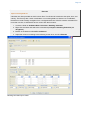
Display a Velocity Profile
1. Right click the new velocity profile and select Map Data in order to see the profile
2. The colors in the profile correspond to the average velocity in the interval between the two
horizon for each shot point.
Page 40
Exercise
Import a velocity data set
Velocities are often provided as ASCII column files. The file should contain the shot point, time, and
velocity. The file may also contain coordinates. In our training data set, there are no coordinates,
therefore we need to assign navigation from a navigation data set. If the file contains velocities from
more than one line, it should also have a column with the line name.
1. Locate the folder 3. Sediment Data / Velocities / Stacking Velocities
2. Right click the folder and select the command object Import > Stacking Velocities (no
navigation)
3. Browse in the data set called ATL-LOS-00.vel
4. Adjust the columns according to the following screen shot, and click Execute
Stacking Velocities import menu
Page 41
Exercise Continued
The data set has now been imported into your project. However it does not yet hold any coordinates.
In order to visualize the stacking velocities with the seismic data, we need to assign navigation to the
velocities. Geocap will use the shot point number in the velocity data set and match them with the
shot points in a navigation file. Either a separate navigation file, or the actual seismic line can be
used as source of navigation. Geocap will match the shot points in the navigation file with the shot
points in the velocity file.
1.
2.
3.
4.
Right click one of the velocity data sets, and select the command object Assign Navigation
Browse to 3. Sediment Data /Seismic Lines and highlight the corresponding seismic line
Click OK
Right click the velocity data set again, and click Map Data
A color map of the velocity data should appear. If you display the seismic line at the same time, you
should be able to see that the velocities match the seismic line.
The velocity data sets should have the exact same name as the seismic line. If this is the case, then
you can use the assign navigation command object on the folder containing the velocity data. You
should then browse in the folder containing the navigation. Geocap will match the data sets by their
name, and assign navigation accordingly. This way you do not need to assign navigation to one and
one data set, but can do them all in one go.
Exercise
Convert Stacking velocities or RMS velocities to Interval velocities
If you have imported stacking velocities or RMS velocities, we need to convert them to interval
velocities before we can use them as input to the Generate Velocity Profile command.
1. Locate the folder 3. Sediment Data / Velocities / Stacking Velocities
2. Right click the folder and select the command object Compute Interval Velocities (Dix
Formula)
The result will be stored in the folder 3. Sediment Data / Velocities / Interval Velocities.
Dix formula will produce interval velocities if it is run on RMS velocities. You may also use this
formula on stacking velocities, and thereby use the stacking velocities as an approximation for RMS
velocities.
Page 42
Exercise
Generate velocity profile from seismic interpretation using interval velocity dataset
This exercise is quite similar to the first exercise in this tutorial. The only difference is that we will
base the velocities on a data set in the project instead of a look-up table
In order to generate the sediment thickness, we need at least an interpretation of the sediment base,
and the seabed surface. Geocap can also use more interpreted horizons if you provide them.
1.
2.
3.
4.
5.
Locate the folder 3. Sediment Data / Velocities / Velocity Profiles
Right click the folder and select the command object Generate Velocity Profile
Browse in the Seismic line, and the interpretation folder in the Input data group box.
Select Use interval velocities from: Data set in Project
Browse in the Interval velocities input data group box.
It is important that the Interval velocity data set has the same name as the corresponding seismic
line. It is also important that the shot point numbering in the velocity file correspond to the shot point
numbering of the seismic line.
Click Execute
If you select folders containing the seismic lines and the velocity data as input instead of the data
sets, Geocap will match the names, and try to generate more velocity profiles in one go. A dialog with
a list of the matching seismic lines will appear.
1. Click OK, and the velocity profiles will be generated in the Velocity Profiles folder
2. Click close in order to close the Generate velocity profile dialog
3. Right click the new velocity profile and select Map Data in order to see the profile
Exercise
Depth Converting horizons
It is possible to to depth convert each horizon in Geocap. Note that this is not the same as creating a
sediment profile. We will do that in the next chapter.
1. Right-click the Velocity profile you have generated and select Calculate Sediment
Thickness.
2. Tick the Depth Convert horizons radio button
3. Click Execute. The depth converted horizons will be placed under 3. Sediment Data / Depth
Converted Horizons
4. Display the horizons and notice how they have shifted upwards. This is because they are now
in depth, not time.
Page 43
N. Sediment Thickness
Introduction
Aim of this tutorial:
1.
2.
3.
4.
Generate Sediment Profile from seismic interpretation
Import Sediment Thickness points from ASCII file
Import Sediment Thickness Grid
Compute Sediment points > 1% of distance to FOS
Exercises
Exercise
Generate a sediment profile
The velocity profile holds all the data necessary to do generate a sediment thickness. It holds both
the interpretations in time, and the interval velocities to use in the interval between the interpretations.
1.
2.
3.
4.
Right-click the a velocity profile, and select Calculate Sediment thickness
Make sure that Calculate Sediment Thickness as been selected.
Click Execute. A new data set will be created in 3. Sediment Data / Sediment profiles.
Right click the new data set, and select Table viewTable view
The x,y and z is the position and the sea depth at that point. The scalar value is the sediment
thickness. The Shot point column is the points corresponding shot point from the seismic line.
1. Click Close in order to close the Table View
2. Right click the data set again, and select Display profile as cross section
A sediment profile should now be displayed, you may need to un-toggle the Velocity display and the
seismic display, if you are still displaying them in order to get a good view of it.
Page 44
Exercise
Import Sediment Thickness points from ASCII file
This exercise will assume that you have an ASCII Column file containing coordinates with sediment
thicknesses. In the exercise we will use a file which is included in the Atlantis Project the file includes
more than one profile.
1.
2.
3.
4.
5.
6.
7.
8.
9.
10.
11.
12.
13.
14.
15.
16.
17.
18.
19.
Locate the folder 3. Sediment Data / Sediment profiles
Right click the folder and select add folder
Add a sub folder with the name of the survey for example ATL-LOS-00
Right click the folder and select Import > ASCII Column… and the ASCII Column import
dialog will appear.
Click the browse button, and select the sediment thickness file located in the Atlantis folder: At
lantis \ Data \ ATL_Sediments.txt
Adjust the number of header lines in your file with the Adjust header Spin box to one. The
header lines should be displayed in the top part of the file preview, while the bottom part of the
file preview should hold the coordinates.
Set the column separator to whitespace
Select coordinate format X Y
Check the Z and the Scalar Columns checkboxes
Check the Additional attributes
Type in Shot point under Additional attributes, and select number, then click Add. A new
column will appear for the Shot points
Set the cell type to Line
Set Separate Data Sets to Value change
Set Schema to Sediment Thickness
Correct file columns for each data column by adjust the spin boxes . x: 3 y: 4 z: 5 Scalar: 6
Shot point: 2 Data separator: 1
click Execute
Click the Close button in order to close the ASCII Column import dialog. The data has now
been imported. Let us display the data:
Right click one of the datasets and select Zoom to data
Right click the data set again, and select Display profile as cross section
Page 45
Exercise
Import Sediment Thickness Grid
The NGDC has made the World sediment thickness grid which is an approximation of the
sediment thicknesses covering the entire world. It is available from the internet with the link: http://ww
w.ngdc.noaa.gov/mgg/sedthick/sedthick.html
Import that grid
1. Open the link in your internet browser. Geocap should be able to import all of the formats
which are presented. For this exercise you may download the GMT NetCDF file.
2. Click the Download GMT NetCDF grd file. Store the file, and Unzip the grid to your hard
drive.
3. Locate the folder 3. Sediment Data / Grids If you do not have this folder you may create it.
Use the generic folder type which is the default option.
4. Right click the folder and select Import > Generic… and the Generic import dialog will appear.
Click the browse button, and select the sediment thickness file.
5. Click the Area of Interest tab. Here you will see extent of the file. You may specify the import
area at the bottom.
6. Check the import area button, type in the coordinates of your area in decimal degrees.
7. Click Execute.
8. You will now be prompted with a question of the coordinate system and datum. Select: World
Geodetic system 1984 Geodetic. Click OK
9. Click close.
The data is imported in Geodetic, with latitudes as Y coordinates and longitudes as X coordinates. In
order to view the data with the other data we have imported need to convert the grid to Mercator
coordinates:
1. Right click the dataset and select Shared commands > Convert to Mercator
2. Change the result combo box to Replace input
3. Click Execute. The data is now converted.
Let us display the data:
1. Right click the dataset and select Zoom to data
2. Right click the dataset and select Map
You should now see the sediment grid in your area.
Page 46
Exercise
Compute Sediment points > 1% of distance to FOS
In the previous exercises we imported and calculated sediment thicknesses. In order to apply the
sediment thickness formula in UNCLOS Article 76, we need to compare the sediment thickness with
the distance to the foot of slope. In this exercise we will cover how you can do this calculation. We
assume that you already have a foot of slope dataset.
1. Right click the sediment thickness data set.
2. Select the command Generate > 1% of distance to FOS A dialog asking for the Foot of slope
data set will appear
3. Browse and select the Foot of slope data-set you want to use for the calculation, click OK.
4. Uncheck the Store in project box
5. Click Execute
If the data-set contained any points thicker than 1% of the distance to the nearest FOS point, it will
display the sediment profile in green. Points less than 1% distance to FOS will be displayed in red.
1. To store the resulting 1% sediment thickness points check the box Store in project
2. Click Execute. A new data set will be created in 3. Sediment Data / Sediment Thickness
Points.
Exercise
Observe the Table View for the Sediment Thickness Points
The table view for sediment thickness points contains a lot of relevant metadata.
1. Right-click the sediment thickness points dataset in the folder 3. Sediment Data / Sediment
Thickness Points and select Table View
2. Observe that that each 1% sediment thickness point refers back to a profile, an analysis and a
FOS point. It also reports the thickness, shot point, distance in m and percent of distance to
FOS.
Page 47
O. Final Outer Limits
Introduction
The construction of outer limits is (obviously) a complex operation. Sometimes it is best to do this area by area
and in multiple steps, then combining points into one or more final outer limits. Sometimes the outer limit line
may be constructed from a combined formula line and a combined constraint line.
The ultimate construction may still be a complex logical and strategical operation. The Geocap Final Outer Limit
tool is designed to digitize to combine line segments and keep distances between points less than 60M.
Exercises
About the Outer Limit Menu
The "Outer Limit Menu" is used in order to select the final outer limit points from the formula and constraint lines.
You may open the outer limit menu by right-clicking on the project folder 4. Outer limit and selecting Generate
Outer Limit.
The Outer Limit Menu
The blue question mark in the top right corner of this menu contains instructions on how to use this menu.
The folders in the Outer Limit menu correspond to the sub folders in 4. Outer limit. You will also be able to see
the datasets in this list. Before opening this menu, you can copy the files you want to use in your outer limit to
the correct folders.
You can display the different data sets by checking the data sets you want to display, and clicking the pencil.
Multiple select is allowed in this list. You can scale the display window to the data sets the same way by
checking the datasets, and clicking the scale button.
The digitize button is used to digitize points from the checked data-sets. You can use this to pick points on your
final outer limit. Each time you pick a point, a white circle of 60M will be displayed around the last picked point.
The circle is geodetic correct. This will be a guide to you when digitizing the final outer limit. The distance
between the final outer limit points should be less than 60M, so the next point you pick should be inside the
circle.
Page 48
Exercise
Try the Outer Limit tool
Before doing the exercise below, get a hand on feeling with the functionality of the digitizer, just by
playing around with two datasets.
Copy the 200M line into 4. Outer limit / Formulae
Copy your 2500m + 100M into 4. Outer limit / Constraints
Display the data from the Final Outer Limits panel. Note that the data may also be displayed
from the project, e.g. Display Points.
Try the various digitizing operations.
Exercise
Generate the Outer Limit
In this exercise we are going to digitize the outer limit from your formula, and constraint lines using
the Outer Limit menu.
1. Copy all your formula lines to the 4. Outer limit / Formulae folder (200M, FOS+60, Sed>1%
points)
2. Copy all your constraint lines to the 4. Outer limit / Constraints folder (350M, 2500m + 100M)
3. Open the Outer limit menu, and check some of the datasets and use the Display and scale bu
ttons
The Outer Limit menu with Datasets Copied
Page 49
Exercise Continued
1. Digitize a combined formula line, by clicking the digitize button and following the instructions
2. When you have finished digitizing and clicked the end digitize button, give the new dataset a
name, such as combined formula line.
3. Right click the new line in the project, and select Table view
4. Observe the new columns in the table
There are also two tools which have been developed in order to Optimize the outer limit and to Maximize the
outer limit. These tools should be used with great care in order for them to be utilized correctly. It cannot be
assumed these tools will automatically produce the absolute maximum achievable area. They are interactive
tools that should be experimented with, using different settings until the desired result is obtained.
The Maximize outer limit panel together with the Optimize outer limit panel
Page 50
P. Uncertainty
Introduction
Exercises
Exercise
Vertical to horizontal uncertainty
In this exercise we will investigate the implications on the 1%-thickness points/area of varying the
sediment thickness. Create alternative sediment thicknesses, either by:
1. Multiplying the thickness by 0.9 to produce a minimum thickness and multiply by 1.1 to
produce a maximum thickness.
2. Change the depth conversion to produce an alternative thickness.
How to vary sediment thickness (uncertainty in thickness)
The thickness along a profile can be adjusted up and down in order to measure the horizontal effect on the 1%
point (1%point is used in the following for the point used in UNCLOS art. 76 where the thickness of sediments
are equal to 1% of the distance to the FOS). FOS = Foot of slope point. If you have a seabed (in depth) and an
interpretation of the base of sediments, you may use formulas or methods in Geocap to depth convert the base
of sediments. If you have used Geocap methods with stacking velocities and Dix interval velocities described in
chapter 17 in the user manual, you will end up with Sediment profiles and Sediment thickness points as
present in the Atlantis project.
Exercise
Vary sediment thickness
Right-click ATL-LOS-00-2 in 3. Sediment Data/Sediment profiles and click Table view
This table contains x, y and z for the seabed bathymetry. The Scaler (S) contains the sediment
thickness. The dataset also contains shotpoint numbers.
Table view (Note the checkbox allowing a visualization of the table entries).
Page 51
Exercise Continued
We want to create a thinner (minimum) profile and a thicker (maximum) profile.
1.
2.
3.
4.
5.
Right-click ATL-LOS-00-2 and click Copy
Right-click on the Sediment profiles folder and click Paste twice.
Name the new datasets ATL-LOS-00-2- max and ATL-LOS-00-2- min
Right-click on ATL-LOS-00-2- max and click Make active
Go to the shell in the toolbox and type: mul sca 1.1
Now, the scalar (i.e. the thickness) is increased by 10%.
1. Right-click on ATL-LOS-00-2- max > Assign from workspace > active
2. Right-click on ATL-LOS-00-2- max > Generate 1% dist to FOS area. (You may be asked for
projection which is Mercator, central meridian 0.)
3. You will be asked for foot of slope point(s), and you can select the FOS's Northern Plateau.
4. Repeat this for ATL-LOS-00-2- min but multiply by 0.91.
The two new datasets that are created have all points on the lines that falls within the 1% thickness
criterion.
Page 52
Q. Gridding
Introduction
Read about gridding in the User Manual. The gridding commands collection can be reached on the right-click
menu on any dataset of schema Poly Data. Below follows a step-by-step procedure for gridding, using the
Seafloor functionality in Geocap.
Exercises
Gridding multibeam XYZ-data in Seafloor
This demo will take you through the steps from importing Multibeam XYZ data to displaying the final grid. The
multibeam XYZ data can be found in the /Data/Seafloor folder in the Atlantis project. Note that the Atlantis
project is in Mercator, central meridian 0.
Exercise
Creating a Seafloor project.
1.
2.
3.
4.
Click File > New > Project
Select the Seafloor project template and a name and path for your project. Click Finish.
Click Seafloor at the menu bar and open the Seafloor Module Main Panel.
Click Settings and Geodetic Settings. Select an appropriate datum and coordinate system
and click OK.
Exercise
Importing data
1. Click Import to XYZ data folder...
2. Import all the XYZ-files with an appropriate import method.
3. You should now be able to see your data in the XYZ data folder under the 1. Survey Data fold
er.
Exercise
Displaying raw point data (soundings)
1.
2.
3.
4.
Right-click the XYZ data folder and select Display Soundings
Select Show soundings, Use colour range and Use same range for all
Select all files (click one and then ctrl + a)
Select Scale to selected files and click Execute
Exercise
Creating a chart
1.
2.
3.
4.
5.
6.
Click Create and Modify Chart
Select the Create Single Chart tab
Click Scale to soundings
Check the box next to the XYZ data folder and click ok
Click Execute
You can now find your chart frame in the Chart folder under the 2. Charts folder.
Page 53
Exercise
Extract soundings
1.
2.
3.
4.
5.
Click Extract Soundings...
Check the box next to the XYZ data folder.
Select the Chart folder so it is marked.
Click Execute
You will now see that the Chart folder has been updated with a Soundings dataset.
Exercise
Gridding chart
1. Click Gridding Chart...
2. Select Parabolic gridding algorithm with an appropriate x-increment and YInc=XInc. Use the
Tools > Distance calculator to find an appropriate increment.
3. Algorithm Parameters may have search radius: 5. Use Boundary Polygon and Automaticall
y Create Boundary Polygon should be checked.
4. Use filter input points and save filtered points with standard deviation, shallow factor: 2 and
deep factor: 2
5. Use Apply smoothing to result grid with convolution, filter width: 1 (3x3) and filter weight:
0.5
6. Select the Chart and click Execute
7. When the gridding has finished you are presented with a dialog box providing you with details
and statistics about the gridding process. At this point, this is not saved, but you can copy and
paste this into a text document.
Exercise
Display chart data
1.
2.
3.
4.
Click Display Chart Data...
Have the following options checked: Frame, Seafloor, Use same range for all and Use LOD
Select the Chart
Have the Scale to selected charts box checked and click Execute
Exercise
Display accepted and rejected points
1. Right-click the Soundings_Accepted dataset in the Chart folder and select Display
2. Select the Soundings Rejected dataset in the Chart folder and right-click the Display comma
nd in the Toolbox
3. Select Edit
4. Check the User Defined Color box and select another color using the Palette
5. Click Execute
Page 54
R. PostScript Plotting
Introduction
PostScript Plotting
Exercises
Start the PostScript plotting panel from Tools > PostScript Plotting.
The panel for PostScript plotting
Read about plotting in Help > Quick Guide to Plotting with Geocap.
Exercise
Generate a plot using your seabed surface as the main dataset.
Follow the steps in the Help > Quick Guide to Plotting with Geocap to produce a plot.
Page 55
S. Workflows
Introduction
A workflow in Geocap is a way of combining datasets and actions or visualizations in sequence to produce
visualizations, movements and powerpoint style 3D presentations. The Atlantis Project is used throughout this
tutorial.
Exercises
Exercise
Examine the workflows provided in the Atlantis project.
1. In Geocap, click File > Open > File, and browse to the Atlantis folder, then open the the
sub-folder called workflow.
2. Double click on the file called Atlantis Basic Workflow.gwf to open it, or single click to
highlight it and then click, Open. This will open the workflow below the project.
Atlantis Basic Workflow
Exercise Continued
1. Examine the contents of the workflow items by clicking on the triangles next to the root folders.
2. Click on the Go to first executable element
icon and then click on the Execute next
element
icon. (This will initialize the basic display settings and nothing will appear in the
display window yet)
3. Click on the Execute next element
icon again and notice everything in the Base map fold
er will be displayed along with a short flight tour (animation).
4. Continue clicking on the Execute next element
icon until you reach the end of the
workflow and observe how different elements of the Atlantis project are displayed.
Following the steps above, open and examine the other workflows in the workflows folder.
Note that the user may also execute each element one at a time by right clicking on the command and
choosing Execute, see the image below.
Page 56
Executing individual commands one by one
Exercise
Create a new workflow
In this exercise we will create a workflow that displays seabed and land and some important lines
from the project.
Click File > New > Workflow. Then a browser pops up.
The workflow is saved as a single file on disk with file extension * .gwf, (Geocap Work Flow). A good
idea may be to create a folder in your project called Workflows and put the workflow there.
1. Press the New Element icon to create the first entry. That may also be achieved by a
right-click New Element.
2. Select the Display
3. Right-click the Display
The Display edit panel
command found in the Commands folder and click OK.
command in the workflow and select Edit. Then this panel pops up:
Page 57
Exercise Continued
In a workflow, you will need to browse in an object from the project. The command usually requires a
dataset to do an action on (such as a type of display).
1. Browse to the coastline folder under 1. Maritime lines, highlight The Kingdom of Atlantis an
d click OK.
2. Choose the display settings you like (color, glue to surface or not, etc.) and click OK again.
3. Right click the element in the workflow and choose Execute. Alternatively, click the Execute ic
on.
4. Examine how your display looks and edit the command if necessary to achieve the results you
want by right clicking on the command and choosing edit.
5. In order to keep your workflow organized it is recommended to change the name of the newly
added commands from Display to something more descriptive like, Display Coastline Yellow
which is done by right clicking the command and choosing Rename.
Note that commands may be copied from Shared commands, Item commands and Schema
commands and pasted into the workflow.
1. Right click the Map sea command in the Toolbox and select Copy
. (It should be located
under Schema Commands if you have selected a Seabed Surface.)
2. Click the Paste
button in the workflow.
3. Again you must edit it and browse your seabed surface into the panel.
4. Remember to save the workflow by clicking
Page 58
T. Image Georeferencing
Introduction
This tutorial will guide you through the process of georeferencing a map. To georeference a map or image you
need 3 tie points. These points should cover as much of the map as possible. In this tutorial we will use a map of
the structural elements of the Norwegian continental shelf, which can be downloaded from Norwegian Petroleum
Directorate website. This map has a graticule showing latitude and longitude which works great as tie points.
Exercises
Exercise
Import an image into your project
1. Create a Generic folder (i.e. a folder with schema Generic) and rename that folder to My
Maps
2. Right-click the My Maps folder and go to Import > Generic. Browse for a *.jpg or a *.png.
3. Make sure the schema of the image set to Image Data.
Exercise
Georeference an image
Use the Georeferencing wizard to georeference an image. Follow the step-by-step procedure below.
Georeferencing step by step
Display the map. You may also have to right-click and Zoom to data
Make sure the image is selected in the project and double-click Geo Reference command in the Toolbox
. Notice that the graphic window was changed to 2D mode.
In the first menu, set geodetic properties of the map:
Set Tie point coordinate format to decimal degrees.
Type in the Lat = 70 and Lon = 0 for the first tie point, click Pick and click on the corresponding point in
the map.
Page 59
Type in the Lat = 70 and Lon = 16 for the second tie point, click Pick and click on the corresponding point
in the map.
Type in the Lat = 62 and Lon = 4 for the third tie point, click Pick and click on the corresponding point in
the map.
Click Next
Evaluate the result. The Deviance at tie point represents the accuracy of the georeferencing. The value
should not exceed more than 1 pixel on each point.
Page 60
Page 61
U. Vertical Image Calibration
Introduction
This tutorial will guide you through creating a vertical calibrated image (VCI) from an old scanned seismic image.
The process can however be performed on any image. All you need are two datasets:
Image
Navigation
We assume you have already imported the image and navigation (or digitized a navigation line).
Open VCI menu
The VCI menu is opened from View > Vertical Image Calibration (XCal in older Geocap versions). The menu
should appear in the same panel as your project, like the screen shot below:
As you can see this menu consists of 3 steps (tabs) that you need to complete in order to complete the vertical
calibration.
Input/Output
1.
2.
3.
4.
5.
Click the Image browse button and select the folder where your image resides.
Select the image you want to vertically calibrate in the drop down box.
Click the Navigation browse button and select the folder where your navigation/digitized line resides.
Select the navigation/digitized line you want to vertically calibrate against in the drop down box.
Click the Result folder browse button and select the folder where you want your vertically calibrated
image to be stored.
Vertical Calibration
The vertical calibration uses a cut off range and 3 calibration points. The cut off range usually starts at 0 and
stops at the max depth/time of your seismic image. Everything above or below this cut off range will be
eliminated from the completed VCI. The 3 calibration points specify the orientation and scale in vertical direction
of the image.
1. Click the 2. Vertical Calibration tab to start the vertical calibration.
2. Set the Stop value in the Vertical Cut Off Range to the max time/depth in your image.
3. Set the first calibration point to 0, click the Pick button and click on the corresponding value to the left in
your image.
4. Set the second calibration point to the stop value in your cut off range, click the Pick button and click on
the corresponding value in the middle of your image.
5. Set the third calibration point to 0, click the Pick button and click on the corresponding value to the right in
your image.
6. Use the Focus buttons to zoom closer to each point and re-pick them for a more accurate selection.
Page 62
You should now see two white horizontal lines across your image. One at 0 depth and one at max depth.
If you want to keep parts of the image above 0 or below the max depth of the seismic image you can do
it by adjusting the cut off range after you have set the calibration points. In the example above we could
set the cut off start to -100. This would preserve the well-information at the top of the image.
Navigation Calibration
1. Click the 3. Navigation Calibration tab to start the navigation calibration
2. Locate the first shot point in your image and find the corresponding shot point in the Tie Points list in the
menu.
3. Select the Tie Point in the list, then click the Pick button and click on the shot point in the image.
4. Locate the last shot point in your image and find the corresponding shot point in the Tie Points list in the
menu.
5. Select the Tie Point in the list, then click the Pick button and click on the shot point in the image. You
should now see a line of points along the shot point line.
6. Continue this process with the points between the start and end points if needed.
Note that everything to the left and right of the dotted line and everything above and below the white lines will be
cut off on the completed VCI.
Click the Save button in order to create the VCI
Display
1. Locate your VCI in your result folder.
2. Right-click the VCI dataset and select
Display
It is possible to do seismic interpretation on the vertical calibrated image. Just open the Tools > Seismic
Interpretation panel and pick the Vertical Calibrated Image instead of Seismic.
It is possible to convert a VCI to a seismic by "Convert to Seismic". Then the result may be exported as
a SEG-Y.
Page 63
Z. Additional Shelf Exercises
Introduction
The following exercises are just suggested for further training topics, and may not be explained in detail.
Exercises
Exercise
Make a movie
Use a workflow or just use a the command Flight Tour to create a movie in avi format.
Exercise
Check my "Shared commands"
Import and activate my shared commands and see if there are commands you do like. My shared
commands are found here: http://andeby.no/geocap Just follow the instructions on the page.
Exercise
Hello World!
Type the following line into the shell and press enter:
qinformation Information "Hello World"
Observe the popup. This is a Geocap GUI (Graphical User Interface). Study the examples in the Ref
erence > QTcl section of the documentation and observe that it is fairly easy to build your own front
ends to Geocap. Combined with the internal scripting language and Tcl, this is a very powerful tool.
Exercise
Install the script system "Area Generator Mini"
Read about the Area generator, download the scripts and follow the step-by-step procedure here: htt
p://andeby.no/geocap
Chop out a portion of the world and build the project.
Exercise
The function command
Try the function command to time-convert your seabed surface.
z = 2000 * z / 1490
Exercise
Composed grid
Use two or more grids of different resolution (e.g. Etopo1 and a multibeam grid) and create a
composed grid. Do an FOS-analysis across this composed grid. Read more about composed grids in
the Article section of the main documentation.
Page 64
Exercise
Combine parts of two bathymetric lines into one single bathymetric profile
Use the Outer Limit Tool to do this.
Copy two ore more bathymetric lines into a sub folder of 4. Outer limit. You may prefere to
create a new folder.
Open the Generate Outer Limit Dialog from the 4. Outer limit folder.
Carefully read the In-panel help under the question mark.
Use the tool and especially option m to digitize a new bathymetric line.
Use this new line for an anayysis.
Exercise
Create a bathymetric profile in a grid using a line
In this exercise we are going to create a bathymetric profile from a digitized or already existing line to
sample the sticky_surface to create a bathymetric profile. The exercise assumes that a seabed
surface is activated as the sticky surface:
Right-click on the surface in the project and select Copy to sticky_surface.
A line of any kind can be used, e.g. a digitized line. To digitize a line, use Tools > Quick Digitizing o
r View > Digitizer
1. Create a new shared command of type Script and rename the command to Generate
Bathymetric profile on sticky surface
2. Enter this content:
mak lin grid sticky_surface
mhi bathymetric_profile
qinformation "Mission accomplished" "New profile is found in
workspace bathymetric_profile"
3. Execute on the line to produce bathymetric profiles.
4. Set the filter on the command to run on Generic folders and Polydata only.
www.geocap.no
Oslo office
Geocap AS
Industrigaten 46 A
0357 Oslo
Norway
Phone: +47 22 95 56 60
Mail: [email protected]
Stavanger office
Geocap AS
Valberget 11
4006 Stavanger
Norway
Phone: +47 51 11 04 32
Mail: [email protected]