Download PlaNet Tutorial and Reference Manual

"!$#&%(')#+* ,.-/010243 56!78!9,:!92<;=!?> 02@'AB
C E DGFH JI LKM
N O PRQPS1UT
VXW:Y[Z]\_^RY+`bac<de_f+chgjiP\habYkglYmn^o\pf+arqs^U\8gjtu[Y[vnwxY+iyW
chqs^o\pglt
z<cb{9|b}+~$4t.\pW
€$abc|b‚:‚:ƒ
wd[dEz |„†…:‡‰ˆ…†Š:ŠR}
Konstanzer Online-Publikations-System (KOPS)
URL: http://www.ub.uni-konstanz.de/kops/volltexte/2006/2009/
ŒŽ
‹ px]‘“’•”—˜– ”:™š‘“– ›œ˜”ž“Ÿy =˜”¡•9‘“¢h£¤¥¢¦™¨§©› =˜”¡•
ª “¢ ¡•«/Ÿy›š¬j¡•”—x– ”†­+§©¢h¬j”©¢“®
¯ §¬°”l™± ‹ ž²/²x³/´µ˜¶¸·—¹©¹“ºh»x¹x¼/½©¼$­+§/¢h¬°”šx¢“®/ºh¾EŸy› =x¢]¿
À Á©¡•’æē›Ÿyē›¡Å¢/”š¬šÆ¡Å¢¦™¨§/›l =˜”¡•_Ç ‘“¢“¡ÉȐ/§©¢h¬j”©¢“®©Ç £¦Ÿ
ÊËÊËÊ Âpž/”l”lÄÂ̵©µ˜ÍÎÍÎÍ[Ç ¡Å¢¦™¨§/›l =˜”¡•_Ç ‘“¢“¡ÉȐ/§©¢h¬j”©¢“®©Ç £¦ŸÏµ©Ð ‹ ž“›¡É™Ñ”Ÿy¢
PlaNet Tutorial and Reference Manual Ò
Dagmar Handke
Ó
Gabriele Neyer
Ô
Lehrstuhl für praktische Informatik I
(Algorithmen und Datenstrukturen)
18/1996
Universität Konstanz
Fakultät für Mathematik und Informatik
ÕÖ
×
Part of this research was supported by the Deutsche Forschungsgemeinschaft under grant Wa 654/10-1.
Universität Konstanz, Fakultät für Mathematik und Informatik, Postfach 5560/D188, 78434 Konstanz, Germany.
e–mail: [email protected], Internet: http://www.informatik.uni-konstanz.de/˜handke/
ETH Zürich, Fakultät für Theoretische Informatik, CH-8092 Zurich, Switzerland.
e–mail: [email protected].
Contents
1 What is PlaNet?
1.1 Introduction . . . . . . . . . . .
1.2 From a user’s perspective . . . .
1.3 From a developer’s perspective .
1.4 Terminology and basic notations
1.5 PlaNet documentation . . . . . .
.
.
.
.
.
.
.
.
.
.
.
.
.
.
.
.
.
.
.
.
.
.
.
.
.
.
.
.
.
.
.
.
.
.
.
.
.
.
.
.
.
.
.
.
.
.
.
.
.
.
.
.
.
.
.
.
.
.
.
.
1
1
2
3
4
5
2 Tutorial
2.1 Getting started . . . . . . . . . . . . . . . . . . . . . . . . . . .
2.1.1 System requirements . . . . . . . . . . . . . . . . . . .
2.1.2 Installing PlaNet . . . . . . . . . . . . . . . . . . . . .
2.1.3 Starting PlaNet . . . . . . . . . . . . . . . . . . . . . .
2.1.4 Preparing the account and setting environment variables
2.1.5 Running the menu . . . . . . . . . . . . . . . . . . . .
2.2 The main menu . . . . . . . . . . . . . . . . . . . . . . . . . .
2.2.1 Principles . . . . . . . . . . . . . . . . . . . . . . . . .
2.2.2 The menu item File . . . . . . . . . . . . . . . . . . . .
2.2.3 The menu item Problem . . . . . . . . . . . . . . . . .
2.2.4 The menu item Instance . . . . . . . . . . . . . . . . .
2.2.5 The menu item Algorithm . . . . . . . . . . . . . . . .
2.3 Example . . . . . . . . . . . . . . . . . . . . . . . . . . . . . .
.
.
.
.
.
.
.
.
.
.
.
.
.
.
.
.
.
.
.
.
.
.
.
.
.
.
.
.
.
.
.
.
.
.
.
.
.
.
.
.
.
.
.
.
.
.
.
.
.
.
.
.
.
.
.
.
.
.
.
.
.
.
.
.
.
.
.
.
.
.
.
.
.
.
.
.
.
.
.
.
.
.
.
.
.
.
.
.
.
.
.
.
.
.
.
.
.
.
.
.
.
.
.
.
.
.
.
.
.
.
.
.
.
.
.
.
.
.
.
.
.
.
.
.
.
.
.
.
.
.
.
.
.
.
.
.
.
.
.
.
.
.
.
6
6
6
6
7
7
8
8
8
9
9
10
13
14
.
.
.
.
.
.
.
.
.
.
.
.
.
.
.
.
.
.
.
.
.
.
.
.
.
.
.
.
.
.
.
.
.
.
.
.
.
.
.
.
.
.
.
.
.
.
.
.
.
.
.
.
.
.
.
.
.
.
.
.
.
.
.
.
.
.
.
.
.
.
.
.
.
.
.
.
.
.
.
.
3 Problem classes in PlaNet
3.1 General Net Graph Problem . . . . . . . . . . . . . . . . . . . .
3.2 Net Graph Problem with a Bounded Number of Nets . . . . . . .
3.3 Net Graph Problem with a Bounded Number of Terminals per Net
3.4 Menger Problem . . . . . . . . . . . . . . . . . . . . . . . . . .
3.5 Okamura–Seymour Problem . . . . . . . . . . . . . . . . . . . .
3.6 Three Terminal Menger Problem . . . . . . . . . . . . . . . . . .
.
.
.
.
.
.
.
.
.
.
.
.
.
.
.
.
.
.
.
.
.
.
.
.
.
.
.
.
.
.
.
.
.
.
.
.
.
.
.
.
.
.
.
.
.
.
.
.
.
.
.
.
.
.
.
.
.
.
.
.
16
16
17
17
17
17
18
4 Algorithms in PlaNet
4.1 Preliminaries . . . . . . . . . . . . . . . . . . . .
4.2 Algorithms for the Menger Problem . . . . . . . .
4.3 Algorithms for the Okamura–Seymour Problem . .
4.4 Algorithms for the Three Terminal Menger Problem
4.5 Algorithms for the General Net Graph Problem . .
.
.
.
.
.
.
.
.
.
.
.
.
.
.
.
.
.
.
.
.
.
.
.
.
.
.
.
.
.
.
.
.
.
.
.
.
.
.
.
.
.
.
.
.
.
.
.
.
.
.
19
19
20
23
29
30
i
.
.
.
.
.
.
.
.
.
.
.
.
.
.
.
.
.
.
.
.
.
.
.
.
.
.
.
.
.
.
.
.
.
.
.
.
.
.
.
.
5 Instance generators in PlaNet
5.1 Generators for the Menger Problem . . . . . . . .
5.2 Generators for the Okamura–Seymour Problem . .
5.3 Generator for the Three Terminal Menger Problem
5.4 Generator for the General Net Graph Problem . . .
.
.
.
.
.
.
.
.
.
.
.
.
.
.
.
.
.
.
.
.
.
.
.
.
.
.
.
.
.
.
.
.
.
.
.
.
.
.
.
.
.
.
.
.
.
.
.
.
33
33
34
34
34
6 Generation and integration of new classes and algorithms
6.1 Generation of new classes . . . . . . . . . . . . . . . . . . . . .
6.1.1 Parameter handling . . . . . . . . . . . . . . . . . . . .
6.1.2 High-level generation of a new class using makeclass
6.1.3 Generation of a new class from scratch . . . . . . . . .
6.2 Implementation of algorithms and instance generators . . . . . .
6.3 Integration of classes, algorithms and instance generators . . . .
6.3.1 The format of classes.def . . . . . . . . . . . . . .
6.3.2 The format of local/Config . . . . . . . . . . . . .
6.3.3 Generation of the executable . . . . . . . . . . . . . . .
.
.
.
.
.
.
.
.
.
.
.
.
.
.
.
.
.
.
.
.
.
.
.
.
.
.
.
.
.
.
.
.
.
.
.
.
.
.
.
.
.
.
.
.
.
.
.
.
.
.
.
.
.
.
.
.
.
.
.
.
.
.
.
.
.
.
.
.
.
.
.
.
.
.
.
.
.
.
.
.
.
.
.
.
.
.
.
.
.
.
.
.
.
.
.
.
.
.
.
35
35
36
36
37
38
39
39
40
41
.
.
.
.
.
.
.
.
.
.
.
.
.
.
.
.
.
.
.
.
.
.
.
.
A An example of a PlaNet log file
42
B Examples for the generation and integration of new classes and algorithms
44
C Internals
C.1 PlaNet directory structure . . . . . . . . . . . . . . . . . . . . . . . . . . . . . . . .
C.2 About Makefiles . . . . . . . . . . . . . . . . . . . . . . . . . . . . . . . . . . . . .
C.3 The skeleton of class xgraph . . . . . . . . . . . . . . . . . . . . . . . . . . . . .
56
56
57
59
D Format of the PlaNet resource file .planetrc
61
E Format of the graph description file
63
F Basic Algorithms
66
G Xgraph methods
G.1 Constructors, destructors, operators
G.2 Graph methods . . . . . . . . . . .
G.3 Faces . . . . . . . . . . . . . . . .
G.4 Paths . . . . . . . . . . . . . . . . .
G.5 Nets . . . . . . . . . . . . . . . . .
G.6 Graphics . . . . . . . . . . . . . . .
G.7 QuadEdge structure . . . . . . . . .
G.8 Parameters . . . . . . . . . . . . . .
G.9 Input/Output . . . . . . . . . . . . .
G.10 Friend functions . . . . . . . . . . .
.
.
.
.
.
.
.
.
.
.
.
.
.
.
.
.
.
.
.
.
H Graphical interface
.
.
.
.
.
.
.
.
.
.
.
.
.
.
.
.
.
.
.
.
.
.
.
.
.
.
.
.
.
.
.
.
.
.
.
.
.
.
.
.
.
.
.
.
.
.
.
.
.
.
.
.
.
.
.
.
.
.
.
.
.
.
.
.
.
.
.
.
.
.
.
.
.
.
.
.
.
.
.
.
.
.
.
.
.
.
.
.
.
.
.
.
.
.
.
.
.
.
.
.
.
.
.
.
.
.
.
.
.
.
.
.
.
.
.
.
.
.
.
.
.
.
.
.
.
.
.
.
.
.
.
.
.
.
.
.
.
.
.
.
.
.
.
.
.
.
.
.
.
.
.
.
.
.
.
.
.
.
.
.
.
.
.
.
.
.
.
.
.
.
.
.
.
.
.
.
.
.
.
.
.
.
.
.
.
.
.
.
.
.
.
.
.
.
.
.
.
.
.
.
.
.
.
.
.
.
.
.
.
.
.
.
.
.
.
.
.
.
.
.
.
.
.
.
.
.
.
.
.
.
.
.
.
.
.
.
.
.
.
.
68
68
69
74
74
78
80
82
83
85
87
88
ii
Chapter 1
What is PlaNet?
PlaNet is a package of algorithms on planar networks. This package comes with a graphical user
interface, which may be used for demonstrating and animating algorithms. Our focus so far has
been on disjoint path problems. However, the package is intended to serve as a general framework,
wherein algorithms for various problems on planar networks may be integrated and visualized. For
this aim, the structure of the package is designed so that integration of new algorithms and even new
algorithmic problems amounts to applying a short “recipe”. Furthermore, our base graph class offers
various methods that allow a comfortable high-level implementation of classes and algorithms.
1.1 Introduction to PlaNet1
The aim of this package is to demonstrate algorithms on planar graphs by means of a graphical user
interface (GUI). The package is implemented in C++ and runs on Sun Sparc stations, and the graphics
are based on the X11 Window System. A demo version and some additional information is accessible
in the World Wide Web at URL http://www.informatik.uni–konstanz.de/Research/Projects/PlaNet/.
Instances for the different algorithmic problems may be generated either interactively or by a random generator, stored externally in files, and read from the respective file again. All instances are
strongly typed, that is, each instance is associated a (unique) algorithmic problem to which it belongs.
This classification of instances is reflected by the GUI: The user cannot invoke an algorithm with an
instance of the wrong type.
Like instances, all algorithms are classified according to the problems they solve, and this classification is reflected by the GUI too. For each algorithmic problem there may be an arbitrary number of
and , let
indicate that
algorithms solving this problem. For two algorithmic problems,
is a special case of . Such relations of problem classes can be integrated into the package and
are then also reflected by the GUI. More precisely, an algorithm solving problem may be applied
not only to instances of type , but also to instances of any type
so that
. In other words,
although all instances and algorithms are strongly typed by the corresponding algorithmic problems,
an algorithm may be applied to any instance for which it is suitable from a theoretical point of view,
even if the types of the algorithm and the instance are different.
ØÙ
ØÚ
1
؆Ù
Ø
ØÞÝ
Sections 1.1 to 1.3 are basically an extract of [NSWW96]
1
Ø
Ú
؆ÙÛÜØ
Ú
Ø
Ø=ÝoÛ1Ø
In Section 1.2, we give an outline of the GUI and summarize the algorithms that have been integrated
so far. The internal structure of the package is designed to support the integration of new algorithms.
As a consequence, developers may insert new algorithms and algorithmic problems by applying a
short “recipe”, which requires no knowledge about the internals. With this goal in mind, the internal
structure of the package has been designed very carefully. In Section 1.3, we introduce our overall
design. The basic notation is given in Section 1.4. In Section 1.5, the available documentation for
PlaNet is specified.
1.2 From a user’s perspective
Ø
Ø
At every stage of a session with PlaNet, there is a current algorithmic problem . The problem
indicates the node in the problem class hierarchy that the user currently concentrates on. In the
beginning, is void, and the user always has the opportunity to replace by another problem in
the hierarchy. A new current problem may be chosen directly from the list of all problems or by
navigating through the problem class hierarchy. In the latter case, a single navigation step amounts
to replacing either by one of its immediate descendants or by one of its immediate ancestors. To
initialize in the beginning, each of the topmost (i.e., most general) problems may be used as an
entry point for navigation.
Ø
Ø
Ø
Ø
Once the current algorithmic problem is initialized, the user may construct a current instance and
choose one or two current algorithms. Afterwards the user may apply these two algorithms simultaneously to the current instance in order to compare their results.
Ø ÝÝ
Ø=Ý
Ø=ÝßÛÜØ
ØàÛáØ Ý Ý
of the instance satisfies
.
An instance may be generated or read from a file only if the type
Analogously, an algorithm may be chosen only if the type
of the algorithm satisfies
.
In particular, this guarantees that the algorithm is suitable for the instance. These restrictions for
instances and algorithms are enforced by the GUI: To select an algorithm the user must pick it out
of a list, which is collected and offered by the GUI on demand. This list contains only algorithms
so that
). Analogously, the lists of random instance
of appropriate types (namely types
generators and of externally stored instances contain only items of appropriate types (types
so that
).
Ø=Ý ÝßہØ
Ø=Ý
Ø=Ý$âkØ
Ø ÝÝ
When applying one or two algorithms to an instance, the GUI shows not only the final results, but
also visualizes the procedure of the algorithms step by step. After each modification of the display,
the algorithm stops for a prescribed wait time. By default, this wait time is zero, and the user observes
only the final result, because the display of the procedure is too fast. The user may change this wait
time to an arbitrary multiple of msec. in order to observe the procedure step by step.
Many algorithms consist of a small number of major steps, for example, preprocessing and core
procedure. For each major step of an algorithm, a separate, auxiliary window is opened. The initial
display of such a window is the result of the former major step or if it is the very first major step
the plain input instance. The procedure of this major step is displayed in the associated window,
and afterwards the window remains open showing the final result of the major step. Therefore, on
termination of the whole algorithm, all intermediate stages are shown simultaneously and may be
compared with each other. The GUI also offers a feature to print the contents of a window or to dump
it to a file in Postscript format. It is also possible to adjust the graphical display according to the user’s
taste. (See Section 2.2 for a detailed description of the GUI.)
2
So far, the algorithmic problems modeled with PlaNet mainly reflect our theoretical research interests.
These problems are the Okamura–Seymour Problem, the Menger Problem, and further versions of the
Menger Problem. (See Chapter 3 for a detailed description of the problems and Chapter 4 for the
algorithms.) These also include new heuristic variations of well known algorithms. In addition there
are various basic algorithms, for example an algorithm that computes the Delaunay triangulation of a
graph and algorithms that generate feasible random instances for the problem classes (see Chapter 5).
1.3 From a developer’s perspective
The implementation relies heavily on the object-oriented features of C++. Here we do not say much
about object-oriented programming; see for example [Mey94] for a thorough description of objectoriented programming, and see [Str91] for a description of C++. Nonetheless, this section is self
contained to as high an extent as possible. Therefore, we first introduce all terminology that we need
to describe the internal design.
Classes. Classes are a means to model abstract data types. For example, the abstract data type
“stack” is essentially defined by the subroutines “push,” “pop,” and “top.” A stack class wraps an
interface around a concrete implementation of stacks (encapsulation), which consists solely of such
subroutines (usually called the access methods of the stack class). Consider a piece of code which
works with stacks and uses this stack class to implement them. In such a piece of code, only the
interface may be accessed; the concrete implementation behind the interface is hidden from the rest
of the code. This allows software developers to adopt a higher, more abstract point of view, simply by
disregarding all technical details of the implementation of abstract data types.
ã
ä
ä
ã
Inheritance. A class may be derived from another class . This means that the interface of
is the same as or an extension of the interface of , even if the concrete implementation behind the
interface is completely different for and . Moreover, an object of type may be used wherever
an object of type is appropriate. For example, a formal parameter of type may be instantiated
by an actual parameter of type . A class may be derived from several classes (multiple inheritance).
Therefore, inheritance may be used to model relationships between special cases and general cases.
Moreover, inheritance may be used for “code sharing,” that is, all code implemented for the access
methods of class may be used by the access methods of class too.
ä
ã
ã
ä
ä
ã
ã
ä
ä
ä
ã ٘å˜æ˜æ˜æ/å ã$ç
Polymorphism. This is another application of inheritance. It means that classes
are
derived from a common “polymorphic” class , but the access methods of are only declared, not
implemented. Here inheritance is simply used to make
exchangeable: a formal parameter
of type is used where-ever it does not matter which of
is the type of the actual parameter.
ä
ãÞÙ å˜æ˜æ˜æ©å ãç
ã9Ù å˜æ˜æ˜æxå ãç
Û
This concludes the introduction into object-oriented terminology. In PlaNet, each algorithmic problem
is modeled as a class, and inheritance is used to implement the relation . The topmost element of
the inheritance hierarchy is the basic LEDA graph class [MN95]. Consequently, each problem class
offers all features of the LEDA class by code sharing.
We paid particular attention to the problem of integrating new algorithms and new problem classes
into the package afterwards. The problem classes and their inheritance hierarchy are described by a
3
file named classes.def, in a high-level language, which is much simpler than C++. The project
makefile scans classes.def and integrates all problem classes according to their inheritance relations and all solvers into the package.
Therefore, integration of a new problem class amounts to inserting a new item in classes.def. In
addition, a file named Config must be changed slightly. When several developers work on the integration of different new problem classes and algorithms in the package simultaneously, each developer
only needs to maintain his/her own local copy of classes.def and of this small file Config; all
other stuff may be shared. (See Chapter 6 for a detailed description of the generation and integration
of new classes and algorithms.)
Besides the advantages of encapsulation discussed above, we also use encapsulation for several other
important design goals, notably the task of separating the code for graphics from the code for the algorithms. Since the GUI displays not only the output of an algorithm but also its procedure, graphics
and algorithms are strongly coupled. However, it is highly desirable to strictly separate algorithms
and graphics from each other. In fact, if this is not done algorithms and graphics cannot be modified
independently of each other, and changing a small part of the package may result in a chain of modifications throughout the package. This means that maintaining and modifying the package is simply
not feasible.
In PlaNet, the graphical display is delegated to the underlying problem class. The process is as follows.
The most general problem class encapsulates a reference to an additional object, which serves as a
connection to the underlying graphic system. Clearly, this object is inherited by all problem classes.
This object has a polymorphic class type, and from this class type another class is derived, which
realizes graphical display under the X11 Window System. To run the package under another graphical
system, it is only necessary to derive yet another class from this polymorphic class. If one or more
algorithms are to be extracted and run without any graphics, a dummy class must be derived, whose
methods are void.
1.4 Terminology and basic notations
All problems considered in this package require that the underlying graph is a directed or undirected
planar graph. For the basic theory of general graphs, planar graphs and algorithms on these we refer
to [Har69], [CLR94] and [NC88]. Here we only give some very basic definitions. A graph consists
of a set of nodes (also called vertices), and a set of edges (or arcs, in case of directed graphs). A
graph is called planar if it can be embedded into the plane without edge crossings. A path in a graph
is an ordered sequence of nodes and edges/arcs, starting and ending with nodes, respectively, so that
no edge/arc appears more than once in the sequence. We often give undirected paths the direction in
which it is traversed. The leading edge of a path is then the last appended edge. A net is simply a set
of nodes. The nodes in a net are called terminals.
Taking the planar embedding of a graph and removing all edges and nodes, the plane separates into
faces. All edges around such a face define a face in the graph. The boundary of a planar graph is also
called outer face.
Triangulations are very important for our creation of random instances. In a triangulation nodes are
connected by undirected edges so that each inner face forms a triangle. A Delaunay triangulation is
4
a special triangulation in which the circle formed by the nodes of each triangle does not contain any
other node of the graph [Ede87].
Most algorithms consider the problem of finding pairwise disjoint paths connecting two terminal nets.
In a solution of a vertex–disjoint path problem each internal node (i.e. not an endpoint) appears in at
most one path. Analogously, in a solution of an edge–disjoint path problem each edge appears in at
most one path.
1.5 PlaNet documentation
The PlaNet documentation consists of this manual and the online help of the GUI. An overview can
also be found in [NSWW96]. In this manual we first provide a tutorial in which we explain how PlaNet
is started and how the GUI works (see Chapter 2). Then, we describe all problems and algorithms that
are integrated up to now (see Chapters 3, 4 and 5). Chapter 6 contains the recipes for the integration
of new classes and algorithms together with numerous examples. Examples of the different files
mentioned in this manual can be found in the appendix (see Appendix A and B). The appendix also
explains the internal structure of PlaNet and the format of the underlying graph description files (see
Appendix C, D, and E). A reference manual of all available graph functions and basic algorithms is
given in the Appendix F, G, and H.
As an online help in the GUI, most menu windows offer a Help button. Clicking on it invokes special
help for the use of that window or special information about the selected item.
The best way to get used to the functionality and concept of PlaNet is to read the introduction (this
chapter), the tutorial (Chapter 2) and then to retry the example (Section 2.3). For the implementation
and integration of new classes and algorithms into PlaNet it is very important to read Chapter 6.
Within this manual the menu items of PlaNet are typed in bold face. Keywords and variables are
typed in italics. Shell commands and source code are typed in typewriter.
5
Chapter 2
Tutorial
This chapter is a concise tutorial for using PlaNet. It is aimed at users not familiar with the system.
First, the actions to make PlaNet run on the machine are described, and then the menu system is
explained in detail. It is concluded by an example.
2.1 Getting started
2.1.1 System requirements
PlaNet can be installed on SUN workstations (SunOS 4.1 and Solaris 2.x), with X11 Release 5 or 6.
To compile PlaNet a gnu C++ compiler (versions 2.6.3, 2.7.0 or 2.7.2) and LEDA 3.0 are required.
The use of a color display is recommended.
2.1.2 Installing PlaNet
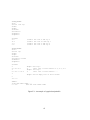
The source code can can be obtained via ftp using the information given in Table 2.1. For the installation also confer the file PlaNet.README. First change to the directory for the LEDA installation
and for the PlaNet installation, respectively. Then use the command tar within these directories to
extract the source files:
Host:
Login:
Password:
Directory:
Files:
ftp.informatik.uni-konstanz.de
anonymous
your email address
pub/algo/executables/planet/
PlaNet.README
PlaNet-vs.tar.gz
LEDA-3.0.tar.gz
è
é
Table 2.1: Ftp adress for the source code
6
cd /path_to_LEDA/
tar xvzf /path_to_tar_file/LEDA-3.0-patched.tar.gz
cd /path_to_PlaNet/
tar xvzf /path_to_tar_file/PlaNet-1.3.tar.gz
The tar files are written such that the top directory is included. Thus, LEDA and PlaNet, respectively, are created in the current directory. For the further installation process of LEDA see
the files README and INSTALL in the LEDA home directory /path_to_LEDA/LEDA-3.0.
For the installation of PlaNet follow the instructions of file README in the PlaNet home directory
/path_to_PlaNet/planet.
2.1.3 Starting PlaNet
PlaNet can be run from any X server, as long as the environment variable DISPLAY is set correctly.
To start up PlaNet, enter
/path_to_PlaNet/planet/planet.
2.1.4 Preparing the account and setting environment variables
Library of instances. PlaNet comes with a default instance library, that is stored in the subdirectory
/path_to_PlaNet/planet/instances. Becoming familiar with PlaNet, it will probably be
necessary to create an own library of PlaNet instances. It is therefore recommended to create a new
directory called planet in the own home directory and a subdirectory instances. In this subdirectory, create a link to the original PlaNet instances, (for example) by using the command
lndir /path_to_planet/planet/instances.
This has the advantage that all built-in instances keep visible and own instances can be stored too. If
the environment variable PLANET_INSTANCES is now set to this instance path, PlaNet will read
instances from and write instances into the new library. The instance path can also be set online in the
submenu File of the main menu (cf. Section 2.2.2).
Default Postscript file. By default, PlaNet uses the filename that is stored in the environment variable PLANET_POSTSCRIPT when the contents of a graph window is to be saved into a PostScript
file. By setting this variable to a full filename, PlaNet will save PostScript output to this filename.
Display of Nodes, Edges and Colors. On a color display, the graphical user interface attempts to
allocate up to 24 colors — or as many as possible if the global color map has been filled up by other
applications (e.g. Netscape). These colors are defined in the PlaNet resource file .planetrc. This
file also defines the node width and line width of the graphs. When started, PlaNet searches for this
file first in the local directory, and if no such file exists, in the home directory. If no such file is found,
default colors are used and a file /.planetrc is created. If the colors or the node/line width are
7
not suitable, this file can be modified accordingly. For a description of the format of file .planetrc
see Appendix D. The colors, the node width, and the line width can also be set in the submenu File
of the main menu (cf. Section 2.2.2). The colors mentioned in this manual refer to the default colors.
2.1.5 Running the menu
PlaNet is a menu driven program where all action can be selected from the given items. For selection
of any menu item click on that item with the left mouse button. For scroll bars also use the left mouse
button to navigate through the given subitems. Most windows offer three buttons: Help, Cancel
and OK. These are initiated by a click with the left mouse button. The Help button gives special
information for the selected item of that window. Pushing the Cancel button leaves the window
without changing the state of PlaNet. By clicking on an OK button the selected item of the window
is set or the action is carried out.
2.2 The main menu
2.2.1 Principles
The state of PlaNet is defined by four items, the Current Problem, the Current Instance, the Current
Algorithm 1, and the Current Algorithm 2. These four items and their current values are always
displayed in the main window. As described in the introduction, an algorithm for the Current Problem
can solve any Current Instance of type
if
is a special case of (i.e.
). Thus, one
or two Current Algorithms may be chosen from a list of all available algorithms of type
with
.
Ø
ØsہØÞÝ
ØÝ ØÝ
Ø
Ø Ý ÛkØ
ØÞÝ
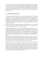
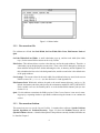
Figure 2.1 shows this main window as it pops up after the start of PlaNet. It consists of the main
menu for the interaction with the system, a listing of the state variables, and the PlaNet log window.
The log window gives a short documentation of all actions of PlaNet. For example, the selection of
a new problem, algorithm or instance are documented there. Furthermore it contains all messages,
warnings and error messages in respect to the use of PlaNet. Especially the results of the algorithms
are documented here. Use the scrollbar on the right side of that window to navigate through all log
messages. Apart from the display in the main menu, all messages are also automatically written to
a log file. The name of this file is displayed in the top of the log window. It is stored in the current
working directory, or if this is not possible in the user’s home directory.
In general, the menu is run by first selecting an item from the menu item Problem, which sets the
Current Problem or both the Current Problem and the Current Algorithm. Then, the Current Instance
is generated by selecting the menu item Instance. Finally one or two Current Algorithms are selected
and made run by operating the menu item Algorithms. Apart from that general course of action, it is
always possible to select another Current Problem, Instance or Algorithm at any stage of the session.
When an instance is selected, it is displayed in a graph window. This window is arbitrarily resizable
and movable, and offers the buttons Close, Redraw, Scale +, and Scale -. Pushing the button Scale
+ (or Scale -, respectively) scales the given instance upwards (or downwards, respectively) within the
given graph window. See Chapter 4 for several examples of a graph window containing instances of
different problem classes.
8
Figure 2.1: Main window
2.2.2 The menu item File
Five subitems are offered: Set Node Width, Set Line Width, Edit Colors, Edit Instance Path and
Quit.
Set Node Width/Set Line Width: A small subwindow pops up, and the node width (line width,
resp.) for the current PlaNet session can be set by a slider.
Edit Colors: This subitem allows to set the colors that are used in the graph windows. Therefore, a
subwindow pops up displaying the current colors. These colors can be changed by clicking on
them and then moving the three sliders indicating the color, its intensity and its brightness. In
this subwindow the first color is the background color, and the second color is the default color
of the graph windows.
Save Settings: The current values for the node width, line width and colors are stored in the current
PlaNet resource file .planetrc (see also Section 2.1.4 and Appendix D).
Edit Instance Path: Within this subitem, the path to the actual instance directory can be set. By
default, the instance path is the path given by the environment variable PLANET_INSTANCES.
If this variable is not set, the instance path is set to the default PlaNet instance path (see also
Section 2.1.4).
Quit: Use this subitem to terminate the PlaNet session. If the Current Instance is not saved a warning pops up, requesting whether to quit PlaNet without saving the instance or to continue the
session.
2.2.3 The menu item Problem
This menu item serves to set the Current Problem. It contains three subitems: Specific Problem,
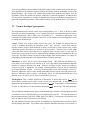
Specific Algorithm and Problem Hierarchy. Figure 2.2 shows the Problem submenu and the
Specific Problem submenu. A detailed description of the problems currently included in PlaNet can
be found in Chapter 3.
9
Figure 2.2: Menu item Problem and a listing of all problems of subitem Specific Problem.
Specific Problem: A list of all available problems is presented in a subwindow. A problem class can
be chosen by clicking on it, and then pushing the OK button. The Help button displays special
information about the selected problem.
Specific Algorithm: A list of all available algorithms and their corresponding problem classes is
presented in a subwindow. By choosing an algorithm, this is taken as the Current Algorithm and
its problem class is taken as the Current Problem. The Help button presents special information
about the selected algorithm.
Problem Hierarchy: A new window pops up visualizing the problem class hierarchy. The left (right,
resp.) subwindow shows the immediate ancestors (descendants, resp.) of the Current Problem
in the problem hierarchy according to the order . The lower window indicates the Current
Problem. It is possible to navigate through the problem hierarchy by a double click with the left
mouse button on the ancestor or descendant with the left mouse button.
Û
2.2.4 The menu item Instance
In this item several routines for handling the Current Instance (like reading an instance from the given
graph database, editing, saving and printing) are offered. It contains the subitems Instance from
Graph Database, Reset Instance, Empty Instance, Edit Graph, Edit Graph Description, Random Instance, Save Current Instance, Save Current Instance as Postscript File, Print Current
Instance, and Test Feasibility. Figure 2.3 shows all subitems of this item and a listing of all Instances
from Graph Database for the Menger Problem (cf. Section 3.4).
ØÝ
Ø Ý Û1Ø
Ø
Instance from Graph Database: Let the Current Problem be of class , then all available instances
from the graph database of problem class
with
are presented in a subwindow. The
path to the graph database can be set by the environment variable PLANET_INSTANCES (see
Section 2.1.4) or in the submenu File/Edit Instance Path (cf. Section 2.2.2). An instance can
be chosen by clicking on it, and then pushing the OK button. The variable Current Instance is
set to the instance name, and the selected instance is displayed in the graph window.
Reset Instance: Use this subitem to reset the Reset Instance to its initial state. If it has been changed
during the session, a warning pops up giving the possibility to cancel the action. If confirmed,
the last instance which has been read from the graph database or generated by item Random
Instance is reloaded.
10
Figure 2.3: Menu item Instances and the listing of all instances for the Menger Problem of submenu
Instance from Graph Database.
Empty Instance: Use this subitem to create an empty instance for the Current Problem. If the Current Instance has been changed during the session, a warning pops up giving the possibility to
cancel the action. If confirmed, the graph window is cleared (or a new graph window is opened).
An empty instance can be used to construct a graph with the menu item Edit Graph.
Edit Graph: This feature allows editing the Current Instance or constructing a new one. Nodes
and edges can be inserted, deleted, or moved around; nets can be added or removed, and all
parameters of the graph, nodes and edges can be edited. To do this, a new window (called
graph editor) containing a copy of the Current Instance is opened. Within this the functions
as indicated in Table 2.2 are available. Thus, for example, to insert an edge, select the source
node, move the pointer to the target node, and press the ’Insert Edge’ key (Shift + mouse button
2). With the right mouse button pressed down, a node can be moved smoothly in the plane. If a
non-planar graph is constructed within this tool, PlaNet will make the graph planar by deleting
some edges. Thus, a planar (but not necessarily plane) graph is achieved. Additionally, the
graph editor menu offers the following buttons:
Place graph in the middle of the window:
Insert Node:
Insert Edge:
Delete Node:
Delete Edge:
Select Node:
Select Edge:
Select node parameters:
Select edge parameters:
Move Selected Node:
SHIFT +
SHIFT +
SHIFT +
CTRL +
CTRL +
ALT +
ALT +
"+"
Mouse Button 1
Mouse Button 2
Mouse Button 1
Mouse Button 2
Mouse Button 1
Mouse Button 2
Mouse Button 1
Mouse Button 2
Mouse Button 3
Table 2.2: Edit functions in the graph editor
11
Use: A window pops up to decide whether the edge of the current graph are directed or undirected. The graph is then transmitted to the graph window as it is displayed in the graph
editor.
Quit: The graph editor is closed, no changes are transmitted to the graph window.
Help: A listing of the edit functions as in Table 2.2 is displayed.
Graph Params: All graph parameters of the Current Problem class are displayed and can be
edited directly.
Node Params: In order to edit the node parameters of a node of the Current Problem class, select it using mouse button 1, and push Node Params. All node parameters of the selected
node are displayed and can be edited directly. There is also a toggle button associated
to each parameter. If this is set, the value of this parameter is copied to all nodes of the
instance.
Edge Params: Editing an edge parameter works analogously to editing a node parameter, except that an edge is selected using mouse button 2.
Nets: All nets of the graph are displayed, each defined by one line. The nodes that belong to
a net are specified by their number in the graph editor. A net that is already present can
be edited directly. In order to add a new net, press the Add Net button. This opens a new
line, and the numbers of the nodes specifying the net (separated by blanks) can be inserted
to specify the net. To delete a net, just delete its nodes in the corresponding line.
Edit Graph Description: The graph description file of the Current Instance is diplayed and can be
edited and manipulated directly. Observe that editing this file is at own risk, since there is no
built-in check routine to maintain its consistency. The format of the graph description file is
described in Appendix E.
Random Instance: A list of all Instance Generators for the Current Problem is presented in a subwindow. Select a generator by clicking on it and pushing the OK button, and a feasible Current
Instance for the Current Problem is created and displayed in the graph window. For a description of the available generators see Chapter 5.
Save Current Instance: A submenu containing the items Save Instance 1 and Save Instance 2 pops
up to select the instance to save. Thereafter, the filename (without the instance path) can be set
in a dialog window. If the instance is of problem class , the instance is written into the
predefined instance directory instances/P using this name and the file format as described
in Appendix E. If a file with this name already exists, a message window pops up to decide
whether to overwrite it or not.
Ø
Save Current Instance as Postscript File: This item works analogously to the previous one, but
here the file name is initially set by the environment variable PLANET_POSTSCRIPT (see
Section 2.1.4). The Current Instance is converted to PostScript format and saved.
Print Current Instance: Again, a submenu containing the items Print Instance 1 and Print Instance 2 pops up to select the instance to print. Thereafter, the printer command can be set in
a dialog window. The Current Instance is then converted to a PostScript file and sent to the
printer by the given command.
12
Figure 2.4: Menu Item Algorithm with subitem Select Algorithm 1 of class Menger Problem.
Test Feasibility: The selection of this item initiate the feasibility test for the Current Instance. For
this purpose, the check routine of the Current Problem class is invoked. For a detailed description of these check routines see Chapter 3.
2.2.5 The menu item Algorithm
This item allows to set the Current Algorithm(s), to make them run and to set the delay of all actions
in the graph windows. It contains the five subitems Select Algorithm 1, Select Algorithm 2, Call
Algorithm, Slow, and 2 Windows (or 1 Window, resp.). Figure 2.4 shows the submenu of menu item
Algorithm and the submenu of subitem Select Algorithm 1 for the current problem class Menger
Problem (cf. Section 3.4).
Ø
ØÞÝ
ØàÛêØ=Ý
Select Algorithm 1: With this item the Current Algorithm 1 can be set. Let the Current Problem be
with
are listed in a subwindow.
of the class , then all available algorithms for
An algorithm can be chosen by clicking on it, and then pushing the OK button. Pushing the
Help button gives a short description of the selected algorithm. For the list of all algorithms see
Chapter 4.
Select Algorithm 2: This item allows to set the Current Algorithm 2. This is done analogously to the
selection of the Current Algorithm 1.
Call Algorithm: If the Current Problem, the Current Instance and at least one Current Algorithm
is selected, the algorithm is called. By default, first the feasibility of the Current Instance is
checked1 . This is done by a call of the check routine of the class that the algorithm was
implemented for (cf. Chapter 3). In case of failure, this is indicated, otherwise the Current
Algorithm(s) are executed. The action of the algorithms is visualized in the main (and some
auxiliary) graph windows. For a detailed description of each algorithm see Chapter 4.
Slow: This menu item allows to set the wait time of the graphical action (in msec) when visualizing
an algorithm: after each modification of the display, the algorithm stops for the given wait time.
Initially, the wait time is set to 0. A delay in terms of 200 msec gives a good insight into the
1
See Section 6.3 how this check can be disabled.
13
algorithmic action. The delay has no effect on Instance Generators chosen by the menu item
Random Instance.
2 Windows: By selection of this item a second graph window is opened and initialized with the
Current Instance. If the algorithms are called now (using menu item Call Algorithm, see
above), both selected algorithms are executed in parallel: Current Algorithm 1 in graph window
1 and Current Algorithm 2 in graph window 2.
1 Window: The selection of this item deletes the second graph window. Using Call Algorithm (see
above), now only invokes Current Algorithm 1.
2.3 Example
In this section, an example for a working session with PlaNet is given. The corresponding log file
of this session (cf. Section 2.1.5) is presented in Appendix A. First, the aim is to solve the Menger
Problem for the instance /user_xy/planet/instances/menger/men30 using the Vertex–
Disjoint Menger Algorithm. In a second step, the solution of this algorithm is compared to the solution
of the Edge–Disjoint Menger Algorithm on a random instance with 20 nodes.
To start the session, call PlaNet (by just typing planet), and the PlaNet main window pops up. As
the goal is to solve the Menger Problem, select both the menu item Problem and the subitem Select
Problem with the left mouse button. A list of all available problems pops up. Select item Menger
Problem, push the Help button to get some more information about this problem, and after reading
this push the Close button. Push the OK button, and the variable Current Problem is now set to
Menger Problem.
To run the algorithm on instance /user_xy/planet/instances/menger/men30, first edit
the instance path: Select menu item File and subitem Edit Instance Path. Now enter /user_xy/planet/instances/ and push OK.
In the next step, select the instance by clicking menu item Instance. A subwindow pops up. Select
item Instance from Graph Database, which pops up a list of all available instances for the Menger
Problem that are stored in /user_xy/planet/instances/menger/. Choose instance men30
and push OK. A graph window showing the instance pops up. The variable Current Instance is now
set to /user_xy/planet/instances/menger/men30.
Now, choose the algorithm by selecting menu item Algorithm and subitem Select Algorithm 1. A
subwindow offering all available algorithms for the Menger Problem pops up. Select Vertex–Disjoint
Menger Algorithm, and push OK. The variable Current Algorithm 1 is now set to this algorithm.
After setting these three variables, the algorithm can be run. To watch the algorithmic action in detail,
select again menu item Algorithm and the subitem Slow. Enter a wait time of 200 msec there, and
push OK. Then, select menu item Algorithm and subitem Call Algorithm to invoke the algorithm.
The algorithmic behavior of the selected algorithm is now visualized in the main graph window and
in an auxiliary graph window. The results are written to the log window and the log file. For a detailed
description of the visualization of the algorithm see Section 4.2. When the algorithm is finished and
the results are studied, close the auxiliary graph window by using the Close button.
14
Now, compare the two algorithms for the Menger Problem on a randomly generated instance with 20
nodes. Therefore, select menu item Instances and subitem Random Instance, which now offers a list
of all available instance generators for the Menger Problem. Choose Generate Random Instance for
Menger Algorithm and push OK. Enter the number of nodes of the instance, 20, and push OK. Now,
a random instance for the Menger Problem is created in the graph window according to the description
of the generator described in Section 5.1. If the instance is not clear enough, try to modify it by using
the graph editor of menu item Instances/Edit Graph. It often helps to scale the instance and to move
some of the nodes.
The aim is now to run the Vertex–Disjoint Menger Algorithm and the Edge–Disjoint Menger Algorithm
in parallel. Therefore, select Current Algorithm 2 to be the Edge–Disjoint Menger Algorithm. This
is done by selecting menu item Algorithms and subitem Select Algorithm 2, then choosing Edge–
Disjoint Menger Algorithm and then pushing OK. As a second graph window is necessary for the
visualization of the Edge–Disjoint Menger Algorithm, select menu item Algorithms and subitem 2
Windows. The selection of item Algorithms and subitem Call Algorithm now invokes the two
algorithms. The results are displayed in their corresponding graph windows and in the log window,
and can be compared. Again, the results are also printed to the log file.
In order to end the session, select item File and Quit, and confirm the warning.
15
Chapter 3
Problem classes in PlaNet
The algorithmic graph problems are modeled as C++ problem classes that reflect the properties of
this algorithmic graph problem. In this chapter the problem classes currently included in PlaNet are
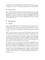
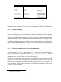
described. The problem hierarchy is given in Figure 3.1, using the internal class names.
Each class has a check routine that tests if the instance is feasible. This is done by first checking the
special properties of the problem class and then calling the check routines of the problem classes the
class is derived from.
3.1 General Net Graph Problem (xgraph)
Graphs in this class are arbitrary planar graphs with an arbitrary number of nets that each contains an
arbitrary number of nodes. The class General Net Graph Problem is the most general planar graph
problem class in PlaNet. Graphs in this class enforce a fixed embedding in the plane. Nodes, edges
and the graph itself can have arbitrary data attached to them. The check routine of this problem
class only checks if the embedding of the graph is planar. This is done by testing all segments on
intersection, thus using quadratic (in the number of edges) running time.
xgraph
bounded_n_nets_graph
menger
bounded_netsize_graph
three_terminal_graph
okamura_seymour_graph
Figure 3.1: Problem hierarchy
16
3.2 Net Graph Problem with a Bounded Number of Nets
(bounded_n_nets_graph)
The class Net Graph Problem with a Bounded Number of Nets is a direct descendant of the class
General Net Graph Problem with the specialization that graphs in this problem class have a bounded
number of nets. The number of terminals in a net remains arbitrary. The number of nets can be set in
the class and is initially bounded to 1.
3.3 Net Graph Problem with a Bounded Number of Terminals per Net
(bounded_netsize_graph)
The class Net Graph Problem with a Bounded Number of Terminals per Net is also a direct descendant
of the class General Net Graph Problem. The graphs in this problem class have a bounded number of
terminals per net; the number of nets remains arbitrary. Initially, the number of terminals per net is
bounded to 2, but can be set to an arbitrary value.
3.4 Menger Problem (menger)
ë
ì
í
ì
í ë
Let be an undirected planar graph with two specified terminals and . The Menger Problem is to
find a maximum number of internally vertex/edge–disjoint paths between and in . Without loss
of generality, here, the embedding of is enforced such that is situated on the outer face of .
ë
í
ë
The class Menger Problem is modeled as a direct descendant of the class Net Graph Problem with a
Bounded Number of Nets and of the class Net Graph Problem with a Bounded Number of Terminals
per Net. The graphs of the class Menger Problem have one net with two terminals and . The
–terminal has to be on the outer face.
ì
í
í
3.5 Okamura–Seymour Problem (okamura_seymour_graph)
ëînï°ð åPñLò
ì©ø íø ùûú1üGúJý
ó?îõô¦ô/ì¦Ù å íö٘÷ å˜æ˜æ˜æ©å ô/ì/ç å íçh÷¦÷
ë
ï°ð åPñJþ ô/ì“Ù å íyÙÏ÷ þÿæ˜æ˜æ“þ ô/ì/ç å íšçh÷ ò
ÙÏå˜æ˜æ˜æ©å bç
Let
be an undirected planar graph with a set of nets
. The
terminal nodes , ,
, are all on the outer face of . Additionally, the so called evenness
condition is fulfilled, that is the extended graph
is Eulerian. The
Okamura–Seymour Problem is to decide whether there are pairwise edge–disjoint paths
,
so that connects with for
, and if so, to determine such a set of paths.
ø
ì©ø
ílø ü:îsù å˜æ˜æ˜æ©å ý
The class Okamura–Seymour Problem is modeled as a descendant of the class Net Graph Problem
with a Bounded Number of Terminals per Net. The graphs of this problem class contain an arbitrary
number of nets with two terminals each. Both of the terminals of each net are on the outer face, each
terminal has degree 1 and all other nodes have even degree.
17
3.6 Three Terminal Menger Problem (three_terminal_graph)
ë
ì¦Ù ì/Ú ì
ô/ì Ù ì Ú ì ÷
Let be an undirected planar graph with three specified terminal nodes , , on the outer face
of . The Three Terminal Menger Problem is to find a maximum number of internally vertex/edge–
, , .
disjoint paths in so that each path connects two nodes out of the given triple
ë
ë
This problem class is modeled as a special case of the class Net Graph Problem with a Bounded
Number of Nets and of the class Net Graph Problem with a Bounded Number of Terminals per Net.
Graphs of this problem class have one net with three terminals which all have to be on the outer face.
18
Chapter 4
Algorithms in PlaNet
In this chapter the algorithms currently integrated in PlaNet are described. These are algorithms
for the Menger Problem, Okamura–Seymour Problem, and for the Three Terminal Menger Problem.
The algorithms are classified according to the problems they solve. As described in the introduction
(Section 1.1), an algorithm working on an instance of class also accepts instances of derived classes
(i.e. classes
with
). Therefore, for each problem class , PlaNet offers algorithms
(
). To avoid redundancy,
that work on instances of class and of more general classes
algorithms are only listed in the description of the algorithms of its most general problem class.
ØÝ
ØÝ
ØÝÛ Ø
Ø
Ø
Ø
Ø=Ý Ý ØáÛsØ=Ý Ý
In the following, we differentiate between problem solving algorithms and basic algorithms. Only the
problem solving algorithms are described in detail. Most of the basic algorithms just form the skeleton
for the built-in instance generators, but they can be used on their own too. By default, before invoking
a problem solving algorithms first a check whether the input instance is feasible is carried out1 . This
is done by the same subroutine that can be called explicitly in the instance menu by choosing subitem
Test Feasibility. Test Feasibility calls the check routine of the problem class that the algorithm is
implemented for.
4.1 Preliminaries
Some underlying basics are explained first for a better understanding of the following. For a detailed
explanation of the following items and especially of most of the following algorithms, see [RLWW95].
Right-first search: Right-first search plays a crucial role within all problem solving algorithms in
PlaNet. This method of searching a graph is a special depth-first search, where in each step all
possibilities for going forward from the leading node are considered in the order “from right to
left”. More precisely, this means the following.
Assume that, at one stage of the search, node is the leading node of the search path, and that
is the leading edge. If there is another edge incident to that is not yet considered at
that stage, the counterclockwise next such edge after in the sorted adjacency list of is
ô å ÷
1
ô å ÷
See Section 6.3 how this check can be disabled.
19
chosen for going forward. A right-first search in a directed graph works analogously, but here
only the arcs that leave the leading node are considered for going forward.
In some of the algorithms in PlaNet, the correctness of the result can be verified easily by computing
a saturated cut or a saturated vertex separator.
Vertex separator: A vertex separator in a connected graph is a set of nodes whose removal disconnects the rest of the graph. Vertex separators can be used to state a necessary condition for an
instance of a vertex–disjoint path problem to be solvable.
ë î"ï°ð åPñò
ì í ð
ò
ì åí
áë
be an undirected graph. A subset is called
Saturated vertex separator: Let
a vertex separator for two nodes , , if and only if and lie in different connected
. We call a vertex separator for and saturated, if every node
components of
is occupied by an ( )–path and no two nodes are occupied by the same
( )–path.
ì åí
ëï°ð
å
ì
ì
í
í
A necessary condition for solvable instances of edge–disjoint path problems in undirected graphs is
the cut condition:
Cut: A cut in a graph is a set of nodes.
Cut condition: If an instance of an edge–disjoint paths problem is solvable, then for every cut in
the underlying graph, the number of edges connecting with is at least the number of
nets with one terminal in and the other one in .
ð
ð
Saturated and over saturated cut: is called an over-saturated cut, if is a cut that does not
fulfill the cut condition. is a saturated cut, if every edge connecting with is
occupied by a different path.
ð
4.2 Algorithms for the Menger Problem
ë
ì
í
ì
í ë
Let be an undirected planar graph with two specified terminals and . The Menger Problem is
to find a maximum number of internally vertex/edge–disjoint paths between and in . Without
loss of generality, here, the embedding of is enforced such that is situated on the outer face of .
Currently, there are two algorithms for the Menger Problem included in PlaNet, the Vertex–Disjoint
Menger Algorithm and the Edge–Disjoint Menger Algorithm.
ë
í
ë
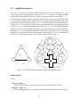
Vertex–Disjoint Menger Algorithm.
Here, the problem is to find internally vertex–disjoint paths in the Menger Problem. In PlaNet the linear time algorithm of Ripphausen–Lipa, Wagner and Weihe is implemented [RLWW93, RLWW97].
See Figure 4.1 for an example.
ì í
In the algorithm, paths from to are routed “as far right as possible”. But a path once determined
by the algorithm needs not necessarily appear in the final solution. Not even an edge that is once
20
ï¥ì å í ò
occupied by an
–path during the algorithm must be occupied by a path of the final solution. Just
the reverse, paths are “rearranged” time and again.
ô å 9÷
ï å ò
í
ï¥ì å í ò
ì í
The algorithm works in a directed, nearly symmetric, auxiliary graph constructed from the undirected
input graph. All edges , except the edges incident to or , are replaced by the two corresponding arcs and . Edges incident to are replaced only by the corresponding arcs leaving ,
and edges incident to are replaced by the corresponding arcs entering . In this auxiliary graph the
directed version of the Menger problem is considered, i.e., the problem of finding as many directed
internally vertex–disjoint
–paths as possible.
ï å ò
ì
Ù å˜æ˜æ˜æxå 8ç
í
ì
í
ì
ü
The algorithm consists of a loop over all arcs leaving . In the iteration, the algorithm
tries to find a path starting with and ending with by right-first search. During the search, conflicts
on the current search path can occur. A conflict occurs when the search path enters another path or
itself. Conflicts are resolved by marking arcs as removed in the graph and rearranging (splitting and
–paths are found. For a more detailed
newly concatenating) the involved paths so that proper
description of the techniques see [RLWW93, RLWW97]. The computed paths are then transformed
into a solution of the original undirected instance.
pø
ï¥ì å í ò
ï¥ì å í ò
After the construction of a maximum set of internally vertex–disjoint
–paths, a saturated vertex
separator is computed by a special depth-first search algorithm. This depth-first search is started from
and using only edges that are not occupied by any path. If a node that is occupied by a path is
entered, the search follows this path one edge backwards and continues. If is reached an extra path is
found. Otherwise, if the search returns back to , a saturated vertex separator consists of the following
nodes: for every visited path take one node with maximum distance from with respect to , and
add the first node of all not visited paths.
ì
í
ì
Ø
ì
Ø
Visualization of the algorithm:
A second window is opened in which the directed graph instance is displayed. There the incremental
construction of the paths can be observed. Every new search path is given a new color. If a path is
split because of a conflict, the back end of the path gets a new color. Analogously, if two paths are
concatenated, the resulting path gets a new color. The resulting paths are then transmitted to the input
instance.
The saturated vertex separator is visualized in the directed graph by marking its nodes in a new color.
All nodes that are visited by the special depth-first search are also marked in a different color. In addition to the graphical information, the vertex–disjoint paths found by the algorithms and the saturated
vertex separator are written to the PlaNet log file and the log window.
Edge–Disjoint Menger Algorithm.
Now, the problem is to find edge–disjoint paths in the Menger Problem. In PlaNet Weihe’s linear time
algorithm is implemented [Wei94, Wei97]. See Figure 4.1 for an example.
ë
The main idea of the algorithm is to reduce the problem to a max flow problem (cf. [CLR94]). Therefore, an auxiliary directed graph is defined, and from this, in a second step, another auxiliary
directed graph are defined. Then, a maximum unit flow from to in is determined, and the
solution is transformed back to a maximum unit flow from to in ! . Finally, the latter flow is
transformed to a maximum number of edge–disjoint
–paths in .
ë
ì í ë
ì í ë
ï¥ì å í ò
ë
21
Figure 4.1: An instance of the Menger Problem, with source 11 and target 16. The left figure shows
the solution constructed by the Vertex–Disjoint Menger Algorithm, the right figure shows the solution
of the Edge–Disjoint Menger Algorithm. In black and white mode the paths belonging to the solution
are dashed.
ë
ë
ô å 9÷ ñ
The graph is the directed, symmetric graph that arises from if each undirected edge "
is replaced with the two corresponding directed arcs and . In the follwing attention is
restriced to the problem of finding a maximum unit flow # from to in , whereby every edge
has capacity 1 and flow 0, initially. To compute the flow in , the second auxiliary graph is
constructed from ! by reversing some edges so that ! does not contain any cycles with clockwise
orientation. Then, a flow in has a 1:1–correspondence to a flow in . The computation of the
flow in works as follows:
ï å ò
ë
ë
ë
ï å ò
ì í ë
ë
ë
ë
ë
Let Ù å˜æ˜æ˜æ/å pç be the arcs leaving ì . The procedure consists essentially of a loop over ù å˜æ˜æ˜æ©å ý . In
the ü iteration, the algorithm routes a path starting with pø and ending with ì or í “as far right as
possible” by right-first search. As every node in ë has even degree the search path always ends in ì
or in í . Every edge is visited only once, the flow of every visited edge is set to 1. Having determined
the maximum flow in ë , the algorithm then reconstructs the flow in ë and the required paths.
Visualization of the algorithm:
A second window is opened where the directed symmetric graph of the instance is displayed. There,
the construction of the residual graph can be observed, where edges are reversed in order to
prevent clockwise cycles. In this residual graph every new search path is given a new color. Now the
flow in is visualized and all edges with unit flow are colored in the main window. Out of these
edges, as many edge–disjoint paths as possible are incrementally constructed and colored. Additional
to this graphical information, the edge–disjoint paths are written to the PlaNet log file and log window
by enumerating the nodes involved.
ë
ë
22
4.3 Algorithms for the Okamura–Seymour Problem
ëînï°ð åPñLò
ì©ø ílø ùLúü[úÿý
ó?îõô¦ô/ì¦Ù å íö٘÷ å˜æ˜æ˜æ©å ô/ì/ç å íçh÷¦÷
ë
ï°ð åPñ1þ ô/ì Ùxå í Ù ÷ þ æ˜æ˜æ“þ /ô ì/ç å íšçh÷ ò
UÙ å˜æ˜æ˜æ©å rç
ø
Let
be an undirected planar graph with a set of nets
. The
terminal nodes , ,
, are all on the outer face of . Additionally, the evenness condition
is Eulerian. The Okamura–
is fulfilled, that is the extended graph
Seymour Problem is to decide whether there are pairwise edge–disjoint paths
, so that
connects with for
, and if so, to determine such a set of paths.
ílø üÎîù å˜æ˜æ˜æ©å ý
ì©ø
One basic Edge–Disjoint Path Algorithm to solve the Okamura–Seymour Problem is included in
PlaNet. In addition, there are also several heuristic algorithms which try to minimize the size of
the solution, i.e. the total length of paths that are found. See [BNW96] or [Ney96] for a detailed
discussion of the heuristics. Figures 4.2 – 4.11 show some algorithmic solutions of an instance. The
basic algorithms given at the end of this section are mainly included for the construction of random
instances.
Problem solving algorithms
Edge–Disjoint Path Algorithm for the Okamura–Seymour Problem.
This is an implementation of the linear time algorithm of Wagner and Weihe [WW93, WW95]. See
Figure 4.2 for an example.
Without loss of generality let all terminals be pairwise different and have degree one2 . We assume that
the terminals satisfy the following condition3 : According to a counterclockwise order starting with an
, and precedes % for
.
arbitrary start terminal $ , precedes for
'&
The solution is now computed in two phases:
ìxø
íø üGînù å˜æ˜æ˜æ©å ý
ï°ë å ó ò
ì í
ü
í
íø
üî ù å˜æ˜æ˜æ©å ý ù
íø RÙ
)(+* with parenthesis structure is constructed. For this,
1. First, a related “easier” instance
consider the , –string of – and –terminals on the outer face in counterclockwise ordering,
starting with a terminal $ . The terminal is assigned a left parenthesis if it is an –terminal,
and a right parenthesis if it is a –terminal. The resulting , –string of parenthesis is then a
string of left and right parenthesis that can be paired correctly. That means that the pairs of
parenthesis are properly nested or disjoint. The terminals are now combined newly according
(-* (i.e. the –terminals remain the same). Then,
to this pairing, choosing
(+* is
solvable, if
is.
¦ý
ï°ë å ó ò
ì
¦ý
íøî í ø
ï°ë å ó ò
í
ü
The procedure to compute the directed paths is essentially a loop over the new nets. In the iteration a path from (-* to (-* ,
is constructed by right-first search. Because the
evenness condition is fulfilled for the instance, each path reaches a –terminal. If the –terminal
is not the problem is not solvable. In this case an over-saturated cut is computed.
ì ø í ø ü9î ù å˜æ˜æ˜æ/å ý
íø
í
í
ï°ë å ó ò
In case of success all computed paths are combined to build the directed auxiliary graph of
instance
with respect to start terminal $ . Therein, all edges of every path are given the
direction in which they are traversed during the procedure.
ü
2. The second phase takes as instance the auxiliary graph and the original nets. Similar to the first
phase, the required paths are computed within a loop over all nets. In the iteration a path
2
3
This is easily achieved by a simple modification of the input instance.
Otherwise exchange start and end terminal of a net.
23
ìxø íø ü.î ù å˜æ˜æ˜æ/å ý
íø
from to ,
, is constructed by right-first search. Again, if is not automatically
reached the instance is unsolvable and an over-saturated cut is computed.
ï°ë å ó ò
Visualization of the algorithm:
Two windows are opened, in both of them the construction of the paths of
)(+* (forming the
auxiliary graph) can be seen. One window stays in this state, the other window visualizes the second
phase of the algorithm. In the . iteration, a path from to ,
is constructed by rightfirst search. Every new path gets the color of its corresponding net. Having computed all paths, these
and their lengths are printed to the PlaNet log file and log window by enumerating the nodes involved.
ìxø íø üEîkù å˜æ˜æ˜æ©å ý
ü
If in any phase of the algorithm the construction of the paths fails, an over-saturated cut is computed
and the edges crossing the cut are colored red. The missing number of edges and the edge identifiers
of the crossing edges are written into the PlaNet log file and log window.
Edge–Disjoint Min Interval Path Algorithm.
This algorithm is a modification of the basic Edge–Disjoint Path Algorithm where the total length of
all paths is heuristically minimized. It uses a sort of preprocessing for the basic algorithm by choosing
the start terminal heuristically before calling it. This heuristic algorithm also has linear running time.
See Figures 4.3, 4.4, and 4.5 for examples.
¦ý
ílø
ì
í
The crucial fact used by the heuristic is that the , –string of – and –terminals on the outer face in
counterclockwise ordering can be shifted cyclically without influencing the solvability of the instance.
Doing this, possibly has to be exchanged with to maintain the property that occurs before in
the string. Now, to every net / an interval of length 0 (for the definition of 0 see below) is associated
and the list is shifted cyclically until the total interval length is minimal. After that, the basic Edge–
Disjoint Path Algorithm is called with the first terminal of the shifted , –string as the start terminal
$ .
ì©ø
‰ø
¨ø
±ø
¨ø
¦ý
ì©ø
íø
The interval length 0 is defined in three ways:
In the first case (Edge–Disjoint Min Interval Path Algorithm I) 0 is the number of terminals between
and in the sequence. In the second case (Edge–Disjoint Min Interval Path Algorithm II) 0 is the
number of edges on the outer face between and . In the third case (Edge–Disjoint Min Interval
Path Algorithm III) 0 is the number of edges on the outer face between and minus the edges
incident to the terminals.
ì©ø
ílø
±ø
ìxø
íø
ø
ìxø
íø
±ø
Visualization of the algorithm:
As this heuristic algorithm differs from the basic Edge–Disjoint Path Algorithm only by using an
especially determined start terminal, the visualization is limited to the indication of the resulting paths
by colors.
Edge–Disjoint Min Parenthesis Interval Path Algorithm.
This algorithm also is a modification of the basic Edge–Disjoint Path Algorithm where the total length
of all paths is heuristically minimized. It again uses a sort of preprocessing by choosing the start
with / being the number
terminal heuristically. This heuristic algorithm has running time 1 /
of nodes and being the number of nets, thus increasing the running time. See Figures 4.3, 4.4, and
4.5 for examples.
ï þ ýÚò
ý
24
ì í
ôhù å˜æ˜æ˜æå ýb÷
As in the Edge–Disjoint Min Interval Path Algorithm above, this heuristic starts at the ordering of
the – and –terminals, in the first phase of the basic algorithm. But now the nets of the problem
with parenthesis structure are considered by associating an interval length 0 to every net / (-* , 2
, of instance
(-* . The definition of 0 is done analogously to the previous algorithm.
ï°ë å ó ò
¨ø
±ø
ø ü
Visualization of the algorithm:
The visualization is done analogously to the heuristic algorithm above.
Reduced Edge–Disjoint Path Algorithm.
In the second phase of the basic Edge–Disjoint Path Algorithm the paths are constructed using only
edges from the auxiliary graph. The Reduced Edge–Disjoint Path Algorithm now uses this by invoking
the basic Edge–Disjoint Path Algorithm first and then removing all edges that are not considered.
Then, a new start terminal is chosen randomly and the basic algorithm is called again with this reduced
instance. This heuristic algorithm again has linear running time. See Figure 4.6 for an example.
Visualization of the algorithm:
First, the result of the Edge–Disjoint Path Algorithm is displayed in the main graph window. A
readable presentation of all paths and their lengths is written to the PlaNet log file and log window.
After that, the result of the Edge–Disjoint Path Algorithm applied to the reduced instance and using
another start terminal is displayed in an auxiliary window. Again, the paths and their lengths are
written to the PlaNet log file and log window.
More Reduced Edge–Disjoint Path Algorithm.
In the method of the Reduced Edge–Disjoint Path Algorithm any terminal can be chosen as start
terminal in the second call of the basic algorithm. This is used in the More Reduced Edge–Disjoint
Path Algorithm by iterating over all possible start terminals. Before every new step, all unused edges
are discarded. This heuristic algorithm has running time 1 3/ with / being the number of nodes
and being the number of nets. See Figure 4.7 for an example.
ï¥ý ò
ý
Visualization of the algorithm:
The solutions of the calls of the Reduced Edge–Disjoint Path Algorithm for each terminal as start
terminal are displayed successively in the graph window. The paths and their lengths of the last
iteration are written to the PlaNet log file and log window. Additionally, the total path lengths of each
iteration are printed.
Edge–Disjoint Path Algorithm — Last/Longest Path Shortest Path.
These two algorithms use a sort of postprocessing for the basic Edge–Disjoint Path Algorithm: The
basic algorithm is called first, and the constructed paths are reconsidered. The aim of this heuristic
algorithm is to make the last/longest path of this solution shorter. Therefore, the last/longest path is
removed from the instance, and recomputed by an algorithm to compute shortest paths using all the
edges of the input instance which are not occupied by the other paths. These heuristic algorithms
again have linear running time. See Figures 4.8 and 4.9 for an example.
Visualization of the algorithm:
The visualization is done analogously to the visualization of the first heuristic algorithm. A readable
representation of the paths and their lengths are written to the PlaNet log file and log window, in-
25
dicating also the number of edges which have been saved by this heuristic in respect to the original
algorithm.
Edge–Disjoint Path Algorithm — All Paths Shortest Paths.
This method again uses a sort of postprocessing for the basic Edge–Disjoint Path Algorithm: The
basic algorithm is called first, and the constructed paths are reconsidered. Let
be the constructed paths. For
to , all paths are successively removed from the graph and recomputed with
an algorithm which determines shortest paths using only edges of the input instance which are not occupied by the other paths. This heuristic algorithm has running time 1 3/ with / being the number
of nodes and being the number of nets. See Figure 4.10 for an example.
UÙ å˜æ˜æ˜æ/å bç
bç UÙ
ï¥ý ò
ý
Visualization of the algorithm:
The visualization is done analogously to the visualization of the previous heuristic.
Min Parenthesis Interval II and All Paths Shortest Paths.
This method is a combination of two of the above heuristics: As a preprocessing, the Edge–Disjoint
Min Parenthesis Interval Path Algorithm II is called, and as a postprocessing, the All Paths Shortest
Path Algorithm is executed. This heuristic algorithm again has running time 1 3/ with / being the
number of nodes and being the number of nets. See Figure 4.11 for an example.
ï¥ý ò
ý
Visualization of the algorithm:
Again, the visualization is done analogously to the visualization of the first heuristic.
Basic algorithms
Generate N Random Terminal Pairs on the Outer Face.
The input of this algorithm should be an instance of the class Okamura–Seymour Problem without
any nets. A dialog window requests the number of nets 4 that are to be generated. The algorithm
then creates ,54 nodes and ,54 edges. Each node is linked to a node on the outer face by an edge, so
that the nodes are uniformly distributed around the outer face of the input graph. Then, the terminals
are randomly combined into two-terminal nets.
Generate Random Terminal Pairs on the Outer Face.
This algorithm works similarly to the algorithm described above. Its input should also be an instance
of the class Okamura–Seymour Problem without any nets. But in this algorithm the number of twoterminal nets is determined by the algorithm: about twice as many nets as there exist nodes on the
outer face of the input instance are generated.
Make every node degree even.
The input for this algorithm should be an instance of the class Okamura–Seymour Problem which
might have nodes with odd degree. The algorithm removes edges from the graph until every node has
even degree except the terminals which are supposed to have odd degree. This is done by listing all
nodes with odd degree (except the terminals). Then, for every two nodes of this list a path between
these nodes is searched heuristically and every edge on the path is deleted.
26
Figure 4.2: The Okamura–Seymour Problem solved by the basic Edge–Disjoint Path
Algorithm. The solution uses 156 edges.
ó î ôpï7658 å 6:9 òöå ï7958 å 9:, òöå ï79:; å 9:< òöå ï76:= å 6?> òöå
7ï 6A@ å 9:9 òöå ï76_ù å 9?> òöå ï79:< å 6:; òöå ï76:6 å 9A@ òöå ï79:6 å 9_ù òöå
7ï 9:= å 6:, ò ÷ . In black and white mode, the paths
Figure 4.3: Result of the heuristic algorithms
Edge–Disjoint Min Interval Path Algorithm I
and Edge–Disjoint Min Parenthesis Interval
Path Algorithm I. The solution uses 130 edges.
belonging to the solution are dashed.
Figure 4.4: Result of the heuristic algorithms
Edge–Disjoint Min Interval Path Algorithm
II and Edge–Disjoint Min Parenthesis Interval Path Algorithm II. The solution uses 125
edges.
Figure 4.5: Result of the heuristic algorithms
Edge–Disjoint Min Interval Path Algorithm
III and Edge–Disjoint Min Parenthesis Interval Path Algorithm III. The solution uses 145
edges.
27
Figure 4.6: Result of the heuristic algorithm
Reduced Edge–Disjoint Path Algorithm. The
solution uses 156 edges.
Figure 4.7: Result of the heuristic algorithm
More Reduced Edge–Disjoint Path Algorithm.
The solution uses 131 edges.
Figure 4.8: Result of the heuristic algorithm
Edge–Disjoint Path Algorithm — Last Path
Shortest Path. The solution uses 143 edges.
Figure 4.9: Result of the heuristic algorithm
Edge–Disjoint Path Algorithm — Longest Path
Shortest Path for the Okamura–Seymour Problem. The solution uses 150 edges.
28
Figure 4.10: Result of the heuristic algorithm
Edge–Disjoint Path Algorithm — All Paths
Shortest Path. The solution uses 84 edges.
Figure 4.11: Result of the heuristic algorithm Min Parenthesis Interval II and All Paths
Shortest Paths. The solution uses 83 edges.
4.4 Algorithms for the Three Terminal Menger Problem
Let B be an undirected planar graph with three specified terminal nodes C:D , CE , CF on the outer face
of B . The Three Terminal Menger Problem is to find a maximum number of internally vertex/edge–
disjoint paths in B so that each path connects two nodes out of the given triple GC D , C E , C FH . Currently,
there are two algorithms included in PlaNet for the Three Terminal Menger Problem, the Three Terminal Vertex–Disjoint Menger Algorithm and the Three Terminal Edge–Disjoint Menger Algorithm.
Figures 4.12 and 4.13 show examples.
Three Terminal Vertex–Disjoint Menger Algorithm.
Here, the problem is to find internally vertex–disjoint paths in the Three Terminal Menger Problem.
Neyer’s linear time algorithm is implemented [Ney96].
Essentially, the algorithm consists of two phases. First, a maximum set of internally vertex–disjoint
paths between any pair of nodes of the given triple GCADJIKCLE5IKCF H is computed independently by rightfirst search. In the second phase, these paths are combined to form a maximal set of internally vertex–
disjoint paths.
The construction of the paths in the first phase is done using the following rule: Let M and N be the
terminals that are to be connected, and O the remaining terminal. If O is on the counterclockwise
path between M and N on the outer face, then the paths are routed from N to M using right-first search.
Otherwise they are routed from M to N . This guarantees that the paths can be combined easily in the
second phase.
For the second phase, observe that a solution of the Three Terminal Vertex–Disjoint Menger Problem
is a subset P of the sum of the independently computed right-first paths between any two terminals
of the triple. The strategy to compute P
now is the following: Let Q (R , S , resp.) be the set of
29
T
T
T
with Q .
CADUIKCELV –paths ( CE?IKCLFLV –paths, CLF?IKCADWV –paths, resp.) as computed in phase 1. Initialize P
Then, add all R –paths (i.e. paths from R ) that are internally vertex–disjoint to P , and repeat this with
the S –paths. Now it is tested whether it is possible to replace one Q –path in P
by a R –path and
a S –path, thus increasing the total number of paths. Because of the construction in phase 1, all the
added R –paths (S –paths, resp.) are the outermost paths of R (S , resp.). Hence, it suffices to examine
only those paths of R and S on being internally vertex–disjoint which are next outermost and not yet
considered. If this is the case, these two paths replace the outermost Q –path in P . This procedure is
repeated until paths are found that are not internally vertex–disjoint.
Visualization of the algorithm:
Three auxiliary graph windows pop up, each visualizing
the incremental construction of one of the
T
three
two-terminal paths of the first phase. The CADIKCLT EV –paths in the first window are colored red, the
T
CEIKCFLV –paths in the second window blue, and the CLF5IKCADXV –paths in the third window green. In the
following the paths are called according to these colors.
The construction of P can be observed in the main graph window. P is initialized with all red paths.
Then all blue paths that are internally vertex–disjoint to P are inserted, and analogously all feasible
green paths are added. After that, the replacement of a red path by a green and a blue path is carried
out if appropriate. In addition to the graphical information, the set P of internally vertex–disjoint
paths with maximum cardinality is written to the PlaNet log file and log window by enumerating the
nodes involved.
Three Terminal Edge–Disjoint Menger Algorithm.
Now, the problem is to find edge–disjoint paths in the Three Terminal Menger Problem. Neyer’s linear
time algorithm is implemented [Ney96]. It works analogously to the previous one, except that edge–
disjoint paths (instead of internally vertex–disjoint paths) are searched in phase 1 and then combined.
The visualization is done in the same way too.
4.5 Algorithms for the General Net Graph Problem
The algorithms in this section were primarily implemented for the construction of random instances.
Generate Random Nodes.
The input for this algorithm should be an empty instance of the class General Net Graph Problem.
The number of nodes Y is requested in a dialog window, and Y nodes on random coordinates are
created. This instance consisting only of nodes is displayed in the graph window.
Delaunay Triangulation.
This algorithm requires the input of an instance of the class General Net Graph Problem that should
not contain any edges. This can be obtained, for example, by using the basic algorithm Generate
Random Nodes or by manual node creation using the Edit Graph feature of the instance menu. The
Delaunay triangulation4 of the nodes is computed and the triangulated graph is displayed. Here, the
algorithm of Guibas and Stolfi is implemented [GS85].
4
See Section 1.4 for the definition.
30
Figure 4.12: A solution of the Three Terminal Vertex–Disjoint Menger Problem. A
maximum set of 6 paths between nodes
G;5Z[I\L]^I\_ H have been determined. In black
and white mode, the paths belonging to the solution are dashed.
Figure 4.13: A solution of the Three Terminal
Edge–Disjoint Menger Problem. A maximum
set of 7 paths between nodes G;5Z[I\L]^I\_ H have
been determined. In black and white mode, the
paths belonging to the solution are dashed.
Triangulation.
As the previous algorithm, this algorithm requires the input of an instance of the class General Net
Graph Problem that should not contain any edges. A random triangulation of the nodes is computed
and the triangulated graph is displayed.
The random triangulation is found by computing a Delaunay triangulation and replacing a random
number ` of edges by their diagonal edge. Here, `bac decgf+h:i!c decjlk , where Znmokpmqc dec is a random
number, and c dec is the number of edges of the triangulation. This method has been suggested by Bill
Thurston (email: [email protected]).
Delete all Multiple Edges.
This algorithm requires the input of an arbitrary instance of the class General Net Graph Problem and
displays it after the deletion of all multiple edges.
Delete N Edges.
This algorithm also requires the input of an arbitrary instance of the class General Net Graph Problem.
The number r is requested in a dialog window, and r randomly chosen edges of the input instance
are deleted. The thus reduced instance is displayed in the graph window.
31
Delete a Random Number of Edges.
Like the previous algorithm, this algorithm requires the input of an arbitrary instance of the class
General Net Graph Problem. A random number ` (Znm`smc decut5v , where c d2c is the number of edges)
of randomly chosen edges of the input instance are deleted, and the reduced instance is displayed.
Create one Net.
The input for this algorithm is an arbitrary instance of class General Net Graph Problem. A net
consisting of two terminals is created where the second terminal is situated on the outer face.
32
Chapter 5
Instance generators in PlaNet
The development of random generators for special planar graph classes is not straightforward and the
design of such algorithms took us a lot of time. All our random instance generators are called with
an empty instance of the corresponding problem class, and consist of the following steps. First, the
number of nodes Y is requested in a dialog window, and Y nodes with random coordinates are created
(algorithm Generate Random Nodes). Then, a triangulation is constructed and afterwards a couple of
edges are removed. The resulting instance is displayed in the graph window.
Note that the triangulations are exactly the maximal planar graphs with respect to the insertion of
edges. Our experience has shown that suitable random distributions can be implemented this way
much more easily than, for example, by constructing random graphs incrementally as it is difficult
to maintain planarity through such a procedure. The following instance generators are included in
PlaNet. The particular algorithms mentioned here are described in detail in the corresponding sections
of Chapter 4 and in Appendix F.
5.1 Generators for the Menger Problem
As described in Section 3.4, a feasible instance of the class Menger Problem consists of an undirected
planar graph with two terminals in one net, and w is on the outer face.
Generate Random Instance for the Menger Problem.
After the creation of the nodes, a random triangulation is computed (algorithm Triangulation). A
random number of randomly chosen
edges is deleted (algorithm Delete a Random Number of Edges),
T
and a random pair of terminals CxIywyV with w on the outer face is created (algorithm Create one Net).
Generate Instance for the Menger Problem.
This instance generator works similarly to the previous one except that the nodes are connected using
a Delaunay Triangulation instead of a random triangulation.
33
5.2 Generators for the Okamura–Seymour Problem
A feasible instance of the class Okamura–Seymour Problem (see Section 3.5) fulfills the following
properties: It is an undirected planar graph with an arbitrary number of two-terminal nets. All terminals have node degree 1 and lie on the outer face, all other nodes have even degree.
Generate Instance for The Okamura–Seymour Problem with N Nets.
After the creation of the nodes, the Delaunay triangulation for these nodes is computed (algorithm
Delaunay Triangulation). Then, a number r of two-terminal nets is requested in a dialog window,
and r terminal pairs are generated being distributed uniformly on the outer face (algorithm Generate
N Random Terminal Pairs on Outer Face). After that, every node degree (except the terminals) is
made even by deleting edges from the instance (algorithm Make every node degree even).
Generate Instance for the Okamura–Seymour Problem.
This instance generator works analogously to the previous one except that the number of nets is
determined by the algorithm Generate Random Terminal Pairs on the Outer Face. This algorithm
generates about twice as many terminals as there are nodes on the outer face.
5.3 Generator for the Three Terminal Menger Problem
An instance of the class Three Terminal Menger Problem (see Section 3.6) has to fulfill the following
properties: It is an undirected planar graph with exactly one net of three terminals. All terminals lie
on the outer face.
Generate Instance for the Three Terminal Menger Problem.
After the creation of the nodes, a random triangulation is computed (algorithm Triangulation), and
three nodes chosen randomly from the outer face are put into a net.
5.4 Generator for the General Net Graph Problem
A feasible instance of the class General Net Graph Problem (see Section 3.1) consists of a planar
graph with an arbitrary number of nets of arbitrary size.
Generate Instance for the General Net Graph Problem.
This algorithm creates a random instance with one net consisting of two terminals. After the creation
of the nodes, the Delaunay triangulation for these nodes is computed (algorithm Delaunay Triangulation), and two randomly chosen nodes are put into a net.
34
Chapter 6
Generation and integration of new classes
and algorithms
PlaNet offers a comfortable way of constructing and integrating new classes and algorithms. In this
section it is described how new classes can be generated easily and how classes, algorithms and
generators are integrated into PlaNet.
The general course of action is the following: For a given problem, first design a C++–class (derived
from class General Net Graph Problem), if all existing classes do not fulfill the properties of the
problem (see Section 6.1). After that, implement the algorithms (see Section 6.2). Then, integrate
the new classes and algorithms into PlaNet. For this PlaNet offers an environment in which classes
and algorithms can be designed in a local source directory and then linked to the PlaNet libraries (see
Section 6.3).
PlaNet allows to choose an arbitrary subset of classes and algorithms from the ones described in this
paper, and to add own new classes and algorithms. There are only three conditions that have to be
fulfilled:
For each algorithm of a problem class {
grated in PlaNet.
z
For each problem class { all more general problem classes {}| of { with {~{}| (up to problem
class General Net Graph Problem) have to be integrated too.
z
z
that is to be integrated into PlaNet, {
has to be inte-
All new problem classes have to be derived from class General Net Graph Problem (directly or
indirectly).
6.1 Generation of new classes
A new class New Class (internally called new_class) to be integrated in PlaNet is specified by two
files: its declaration in the header file new_class.h, and the implementation file new_class.cc.
PlaNet offers a high-level feature with that these files can be generated easily in most cases. But,
35
Data Type (LEDA)
int
float
node
edge
list<int>
list<float>
list<node>
list<edge>
Name in the description file
INT
FLOAT
NODE
EDGE
INTLIST
FLOATLIST
NODELIST
EDGELIST
Comment
LEDA node
LEDA edge
LEDA list of ints
LEDA list of floats
LEDA list of nodes
LEDA list of edges
Table 6.1: Supported data types and their names for graph, node and edge parameters
sometimes it is necessary to write the code for the class from scratch. Here, first the general parameter
handling is explained. Then the design of new classes with and without the high-level tool is described.
6.1.1 Parameter handling
All new graph classes are derived from a base class that is already integrated in PlaNet. All these
classes can automatically manage several data types for parameters on the graph, nodes, and edges.
This means that the parameters and their types only have to be defined in the constructor of the class,
and the base class then allocates and deallocates the space for these parameters automatically when
an instance of the class is created. Furthermore, all parameters and their values are copied by a call of
the copy–constructor of the class. For each parameter it can also be marked there whether it is to be
saved in an output file stream or read in from an input file stream. All parameters can also be edited
by the menu item Graph Edit. Table 6.1 contains a list of all data types that are supported by the
classes in PlaNet. Appendix G.8 lists all available functions on these parameters.
6.1.2 High-level generation of a new class using makeclass
As the creation of a new graph class runs schematically in many cases, PlaNet offers a high-level
environment, called makeclass, which generates C++–code from a high-level description of the
class. It is a perl–script1 , located in the directory /path_to_planet/planet/bin. It can be
used as a self-contained design tool for a new class, if this class only enforces simple parameter
handling, by simply calling it together with the class description file.
Such a class description file consists of five blocks: A definition of the class name, the name of the
base classes it is derived from, and the listings of its graph/node/edge parameters, respectively. Each
of the last three blocks may also be omitted if no such parameter is desired. Lines starting by # are
taken as comments. In each block the information is given by the corresponding keyword in form of
a function. These keywords are:
1
Confer the perl manual pages.
36
# class name
class("foo");
# as we all know, a "foo" is a "bar" and a "fnord"
is_a("bar", "fnord");
# graph parameters
graph_param("source", NODE, SAVE);
graph_param("target", NODE, SAVE);
graph_param("forbidden", NODELIST);
# don’t save the nodelist
# node parameters
node_param("cap", FLOAT, SAVE);
node_param("excess", FLOAT);
# don’t save node excess
# edge parameters
edge_param("cap", FLOAT, SAVE);
Figure 6.1: File foo.def
class("name"): The internal name of the class is name.
is_a("class_1", "class_2", €J€J€ ): The class is derived from class_1, class_2, €J€J€
graph_param("name", type, SAVE): The class has a graph parameter called name of type
type. See Table 6.1 for the supported data types and their names. The parameter SAVE is
optional. If it is given the parameter will be stored (read, resp.) when the instance is written to
(read from, resp.) a file.
node_param("name", type, SAVE): Same as above for node parameters.
edge_param("name", type, SAVE): Same as above for edge parameters.
See Figure 6.1 for the description file called foo.def for the example class foo. The class foo is
derived from class bar and class fnord. The graph parameters are a node called source, a node
called target and a list of nodes called forbidden. The target and source node are to be saved,
while the list of forbidden nodes is not to be saved, when the graph is written to a file. There are two
node parameters of type float called cap and excess (where only cap is to be saved), and one
edge parameter of type float called cap (also is to be saved).
Now, by a call of makeclass foo.def, two files foo.h and foo.cc containing C++–code
are generated. These offer (additionally to all inherited functions of the base classes) all access and
lookup functions for the graph/node/edge parameters as they are defined in foo.def. See Appendix
B (in Figures B.1 and B.2) for a listing of these files.
6.1.3 Generation of a new class from scratch
If a new class that is to be integrated in PlaNet needs more sophisticated modifications (e.g. new
functions and methods), the use of makeclass is not sufficient. But even then the makeclass
feature can help to build a skeleton for the header file and the implementation file of the new class:
37
The files generated by makeclass only have to be extended to contain the additional features of the
class.
In general, when designing a new class without makeclass, it is advisable to encapsulate the header
file of the class description with the header
#ifndef __<classname>_h__
#define __<classname>_h__
and the footer
#endif
Thus, declarations of a header file are included only once in a compilation environment. This is done
automatically by makeclass.
As an example consider a variant of the Menger Problem, the (s,t)–Planar Menger Problem. Here the
problem is to find as many internally vertex–disjoint paths between the two terminals C and w as possible, in instances where both, C and w , lie on the outer face. Thus, feasible instances for this problem
have to fulfill all conditions as the instances of the class Menger Problem, but now also C is restricted
to be on the outer face. Thus, the class (s,t)–Planar Menger Problem is a specialization of class
Menger Problem, and therefore the class menger_s_t_planar is derived from class menger.
There only has to be added a new check routine which tests if the C –terminal lies on the outer face
and then calls the check routine of its base class menger. As this class requires additional tests and
the makeclass feature cannot be used. Figure B.3 and Figure B.4 in Appendix B show the header
file and the implementation file of this class.
6.2 Implementation of algorithms and instance generators
As a class, an algorithm2 New Algorithm, internally called new_algorithm, that is to be integrated
in PlaNet is specified by two files: its declaration in the header file new_algorithm.h, and its implementation in the implementation file new_algorithm.cc. It has to be declared in the following
way:
int new_algorithm(class_A& G);
where class_A is derived from class xgraph or its derivatives (class_A ~ xgraph). A function declared like this certainly also accepts class objects of classes derived from class_A.
All methods of the base classes may be used for the implementation of the algorithms. For a detailed
description of these methods confer Appendix G and H. Additionally, most of the basic algorithms
used in the algorithms currently included in PlaNet can be called also. These are described in Appendix F.
2
or instance generator
38
As an example, consider again the (s,t)–Planar Menger Problem from the previous subsection. Figure B.5 in Appendix B shows the header file menger_s_t_planar_algorithm.h for the (s,t)–
Planar Menger Algorithm. Again, the declaration of the algorithm is encapsulated in a #ifndef
header and #endif footer (cf. Section 6.1.3).
In Figure B.6 in Appendix B, the implementation of the algorithm in file menger_s_t_planar_algorithm.cc is presented. The (s,t)–Planar Menger Algorithm consists of three procedures. The main procedure menger_s_t_planar_algorithm is called by PlaNet with an instance of the class (s,t)–Planar Menger Problem or of a class derived from it. First, the terminals C and
w are extracted from the data structure. Then, the edge that is the first on the path from C to w along the
outer face in counterclockwise direction is determined. After that, the core procedure right_paths
is called with this edge as input parameter.
The procedure right_paths mainly consists of a loop over all edges that are adjacent to C , starting
with edge start. In each iteration, a path from C to w or back to C is searched by a call of procedure
next_path. Procedure next_path now searches a path from C to w as far right as possible by
right-first search. Nodes that have already been visited are marked in a LEDA node_array. The
visualization of the algorithm is done automatically by the underlying graph classes: The terminals of
the net are marked by a color and each path is given another color.
6.3 Integration of classes, algorithms and instance generators
The general course of action when integrating classes, algorithms and generators into PlaNet is the
following: The problem classes and their inheritance hierarchies are described in a high-level language
in a file named classes.def. Then, a file Config is used to indicate local source objects. These
files are then scanned when the actual PlaNet executable is generated by using the make feature.
In order to use this environment, create the following configuration files in the local PlaNet directory:
classes.def, Config, and Makefile. This is done best by copying the template files from the
directory /path_to_planet/planet/config and then modifying these appropriately.
6.3.1 The format of classes.def
In file classes.def, all classes and algorithms of the local version of PlaNet are defined. It consists of a header defining the local PlaNet working directories, followed by a block of lines for each
problem class. Each such block contains the basic information for the class and all its algorithms and
generators. The specific format of the file is as follows. Lines starting with # are taken as comments.
The header consists of the keywords TOP: and the optional keyword LOCAL_SRC:. After the keyword TOP: the path to the PlaNet directory is specified, and after LOCAL_SRC: the path to the local
sources directory, which will also be searched for include files. The current working directory is taken
as a default for LOCAL_SRC. All paths in classes.def have to be specified relative to one of the
paths specified after TOP: or LOCAL_SRC:.
Each problem class block consists of lines starting with the keywords CLASS, INCLUDE:, NAME:,
INSTANCES:, HELP:, followed by a list of algorithms and generators, and is terminated by the
keyword END. The name after CLASS defines the internal class name. All its base classes are listed
39
LOCAL_OBJECTS = ../local/menger_s_t_planar.o \
../local/menger_s_t_planar_algorithm.o
Figure 6.2: An example of a Config file
(separated by blanks) after a “:”. Keyword INCLUDE: is followed by the name of the include file,
i.e. the file containing the declaration of the class. After keyword NAME: the name of the problem as
it is displayed in the graphical user interface of PlaNetis specified. Keyword INSTANCES: indicates
the name of the instance directory for the problem class. After keyword HELP: the name of the
documentation file for the class is expected. The text in this file will appear as help text in PlaNet.
After these lines, a list of algorithms and generators for the problem class may follow. The definition of
an algorithm and a generator differs only in the keyword ALGORITHM or GENERATOR, respectively.
Each list item again consists of lines starting with the keywords ALGORITHM (resp. GENERATOR),
INCLUDE:, NAME:, HELP: and the optional keyword NOCHECK (in case of an algorithm).
After keyword ALGORITHM (resp. GENERATOR) the name of the algorithm is specified. Again, after
keyword INCLUDE: the name of the include file is given. Keyword NAME: indicates the name of
the algorithm as it is displayed in the graphical user interface of PlaNet. The name after keyword
HELP: defines the name of the documentation file for the algorithm. The text in this file will appear
as help text in PlaNet. By default, before an algorithm is called, the current instance is checked on
being feasible. This is done by a call of the check routine of the problem class the algorithm was
implemented for. This call is avoided if the description of the algorithm ends with keyword NOCHECK.
Figure B.7 in Appendix B shows
an example of a classes.def file. There, the set of problem
T
classes consists of the classes CxIywyV –Planar Menger Problem (cf. Section 6.1.3), Menger Problem
and all base T classes thereof. The set of algorithms only consist of the (s,t)–Planar Menger Algorithm
to solve the CxIywyV –Planar Menger Problem, and the Edge–Disjoint Menger Algorithm and the Vertex–
Disjoint Menger Algorithm to solve the Menger Problem. As a generator for the Menger Problem, the
algorithm Generate Random Instance for Menger Algorithm is invoked. In this example, checks for
feasibility of the instances are only carried out before calling the Vertex–Disjoint Menger Algorithm
and the (s,t)–Planar Menger Algorithm.
6.3.2 The format of local/Config
In order to generate an own executable, the Config file also has to be modified. In this file the make
variable LOCAL_OBJS can be set. LOCAL_OBJS must contain all additional object files that are to
be linked into the PlaNet executable; if this variable is not set correctly, the linker will complain about
“undefined symbols” or the like.
Figure 6.2 shows an example of a Config file for one local algorithm called menger_s_t_planar_algorithm.cc, which operates on a graph class called menger_s_t_planar (cf. Section 6.1.3). The source code for this algorithm is located in the directory /my/local/home/src/planet/local, as declared in file classes.def of Figure B.7.
40
6.3.3 Generation of the executable
All that remains is to compile the code and do the linking according to the information given in
the files classes.def and Config. This is done by using the make feature and appropriate
Makefiles which scan the given files (for example, see [OT93] for a detailed description of make).
It is either possible to use the default Makefile that comes with the package, or to write an own,
local Makefile.
To use the default Makefile type make in the local sources directory and make will recurse into all
subdirectories as specified in Config, and try to compile the code there by using a default rule. It is
also possible to carry out only parts of the linking by calling make together with a special target. See
Appendix C.2 (and in particular Paragraph planet/config/Makefile) for a list of these targets
and more information about Makefiles that are builtin in PlaNet.
When writing an own, local Makefile, the path to MakePaths has to be specified in the header.
The file MakePaths should be in the PlaNet home directory.
Anyway, if a Makefile is placed in a local source directory, this one will be used when generating
an executable.
41
Appendix A
An example of a PlaNet log file
Figure A.1 displays the PlaNet log file (cf. Section 2.1.5) of the PlaNet example session as described
in Section 2.3.
42
planet: logging messages to planet-log.2249
planet:
planet:
planet:
planet:
planet:
problem name: Menger Problem.
new instance path: /homes/combi/neyer/planet/instances/
’/homes/combi/neyer/planet/instances/menger/men30’ read.
algorithm 1: Vertex-Disjoint Menger Algorithm
delay set to 200msec.
planet: running ’Vertex-Disjoint Menger Algorithm’...
The following paths were computed:
path 1: [11][17][7][18][24][16]
path 2: [11][2][8][12][20][4][29][6][9]
[1][15][16]
path 3: [11][13][0][19][16]
path 4: [11][5][10][21][16]
Number of paths: 4
Saturated Nodeseperator: [17][20][0][5]
planet: ’Vertex-Disjoint Menger Algorithm’ finished.
planet:
planet:
planet:
planet:
random instance generator called.
’/tmp/.P_AAAa02249’ written.
algorithm 2: Edge-Disjoint Menger Algorithm
switched to 2 window mode.
planet: running ’Vertex-Disjoint Menger Algorithm’...
The following paths were computed:
path 1: [0][18][19][11][6][9]
path 2: [0][14][12][15][17][13][9]
path 3: [0][4][5][1][16][9]
Number of paths: 3
Saturated Nodeseperator: [18][12][16]
planet: ’Vertex-Disjoint Menger Algorithm’ finished.
planet: running ’Edge-Disjoint Menger Algorithm’...
1 path: [0][18][19][11][6][9]
2 path: [0][14][18][7][11][9]
3 path: [0][4][1][12][15][17][13][9]
4 path: [0][10][3][16][9]
Number of paths: 4
planet: ’Edge-Disjoint Menger Algorithm’ finished.
Figure A.1: A PlaNet log file of the example session
43
Appendix B
Examples for the generation and
integration of new classes and algorithms
This chapter contains the files that have been used to illustrate the design and implementation of
new classes and algorithms in Chapter 6. In Section 6.1.2, a class foo.def has been defined as an
example of the use of the makeclass feature. Figures B.1 and B.2 now present the output files
foo.h and foo.cc of the command makeclass foo.def.
T
Figures B.3 and B.4 show the header file and the implementation file of the class CxIywyV –Planar Menger
Problem (called menger_s_t_planar) of Section 6.1.3. This class has been derived from scratch
without using makeclass.
In Section 6.2, the algorithm (s,t)–Planar Menger Algorithm has been described. Figures B.5 and
B.6 show its header and implementation file. It is called menger_s_t_planar_algorithm
internally.
Figure B.7 shows an example of a classes.def file as it is described in Section 6.3.1.
44
#ifndef __foo_h__
#define __foo_h__
// file: foo.h
// Code for class foo generated by makeclass
#include "bar.h"
#include "glompf.h"
class foo :
virtual public bar,
virtual public glompf
{
// indices for accessing parameters
int _node_excess_index;
int _node_cap_index;
int _edge_cap_index;
int _graph_source_index;
int _graph_forbidden_index;
int _graph_target_index;
public:
// constructor & copy constructor
foo();
foo(const foo& G);
// parameter access functions
float get_excess(node v);
void set_excess(node v, float value);
float get_cap(node v);
void set_cap(node v, float value);
float get_cap(edge e);
void set_cap(edge e, float value);
node get_source();
void set_source(node value);
list<node>& get_forbidden();
node get_target();
void set_target(node value);
};
#endif
Figure B.1: File foo.h
45
// file: foo.cc
// Code for class foo generated by makeclass
#include "foo.h"
// constructor & copy constructor
foo::foo() {
_node_excess_index = new_node_float_par("excess", 0);
_node_cap_index = new_node_float_par("cap", 1);
_edge_cap_index = new_edge_float_par("cap", 1);
_graph_source_index = new_graph_node_par("source", 1);
_graph_forbidden_index = new_graph_nodelist_par("forbidden", 0);
_graph_target_index = new_graph_node_par("target", 1);
}
foo::foo(const foo& G) {
_node_excess_index = G._node_excess_index;
_node_cap_index = G._node_cap_index;
_edge_cap_index = G._edge_cap_index;
_graph_source_index = G._graph_source_index;
_graph_forbidden_index = G._graph_forbidden_index;
_graph_target_index = G._graph_target_index;
}
// node parameters...
float foo::get_excess(node v) {
return node_float_par(v, _node_excess_index);
}
void foo::set_excess(node v, float value) {
node_float_par(v, _node_excess_index) = value;
}
float foo::get_cap(node v) {
return node_float_par(v, _node_cap_index);
}
void foo::set_cap(node v, float value) {
node_float_par(v, _node_cap_index) = value;
}
46
// edge parameters...
float foo::get_cap(edge e) {
return edge_float_par(e, _edge_cap_index);
}
void foo::set_cap(edge e, float value) {
edge_float_par(e, _edge_cap_index) = value;
}
// graph parameters...
node foo::get_source() {
return graph_node_par(_graph_source_index);
}
void foo::set_source(node value) {
graph_node_par(_graph_source_index) = value;
}
list<node>& foo::get_forbidden() {
return graph_nodelist_par(_graph_forbidden_index);
}
node foo::get_target() {
return graph_node_par(_graph_target_index);
}
void foo::set_target(node value) {
graph_node_par(_graph_target_index) = value;
}
Figure B.2: File foo.cc
47
//******************************************************************************
//******************************************************************************
//******************************************************************************
// Name of the class: menger_s_t_planar
// Author: Gabriele Neyer
// Date: 25.03.96
//
// About the class:
// The (s,t)-planar Menger Problem
//
// Let G be an undirected planar graph with two specified
// terminals s and t on the outer face.
// The (s,t)-planar Menger Problem is to find maximum number
// of internally vertex/edge-disjoint paths between s and
// t in G.
//
// The class menger_s_t_planar is modeled as a direct
// descendant of class Menger.
// The graphs of this class have one net with two terminals
// s and t. The s and t have to lie on the outer face.
// These properties can be checked by the check-routine
// of the problem class.
//******************************************************************************
//******************************************************************************
//******************************************************************************
#ifndef __menger_s_t_planar_h__
#define __menger_s_t_planar_h__
#include "menger.h"
class menger_s_t_planar :
{
public:
virtual public menger
// constructor & copy constructor
menger_s_t_planar() {};
menger_s_t_planar(const menger_s_t_planar& G) :menger(G){};
// checks if s lies on the outer face and calls ::menger.check(G)
virtual bool check();
};
#endif
Figure B.3: File menger_s_t_planar.h
48
//******************************************************************************
//******************************************************************************
//******************************************************************************
// Name of the class: menger_s_t_planar
// Author: Gabriele Neyer
// Date: 25.03.96
// Modifications:
// For a short description of the class see corresponding ".h"-file.
//******************************************************************************
//******************************************************************************
//******************************************************************************
#include "menger_s_t_planar.h"
// checks if s lies on the outer face and calls ::menger.check(G)
bool menger_s_t_planar::check()
{
if(!menger::check())
return false;
// determine s-terminal (first terminal of the first net of G
node s = first_net()->first();
edge e;
forall_adj_edges(e,s,*this)
// s has to ly on the outer face
if (left_face_id(e)==(int)OUTER_FACE || right_face_id(e)==(int)OUTER_FACE)
return true;
return false;
}
Figure B.4: File menger_s_t_planar.cc
49
//******************************************************************************
//******************************************************************************
//******************************************************************************
// Name of the algorithm: menger_s_t_planar_algorithm
// Author: Gabriele Neyer
// Date: 25.03.96
//
// About the algorithm:
// Menger-s-t-planar Algorithm
//
// a maximum number of internally vertex-disjoint paths
// between s and t is determined by right first search,
// whereby s and t lie on the outer face of graph G.
//******************************************************************************
//******************************************************************************
//******************************************************************************
#ifndef __menger_s_t_planar_algo_h__
#define __menger_s_t_planar_algo_h__
#include <menger_s_t_planar.h>
int menger_s_t_planar_algorithm(menger_s_t_planar& G);
#endif
Figure B.5: File menger_s_t_planar_algorithm.h
50
//******************************************************************************
//******************************************************************************
//******************************************************************************
// Name of the algorithm: menger_s_t_planar_algorithm
// Author: Gabriele Neyer
// Date: 25.03.96
// Modifications:
// For a short description of the algorithm see corresponding ".h"-file.
//******************************************************************************
//******************************************************************************
//******************************************************************************
#include "menger_s_t_planar_algorithm.h"
#include <gui_utils.h>
#include <LEDA/array.h>
// starting at a given edge prev a path from s to t is searched
// by the right first search method, only using unvisited nodes.
int next_path(node s, node t, edge prev,
node v, path P, node_array<int>& visited,
xgraph& G )
{
node w;
int found = 0;
edge succ = G.cyclic_adj_succ(prev, v); // next counterclockwise edge to prev
do
{
if((w=G.target(succ))==v)
// determine source and target of succ
w=G.source(succ);
if(w == t )
// (s,t)-path found
{
G.append(P,succ);
return 1;
}
if(w==s)
return 0;
if(visited[w]==0)
// node w is unvisited
{
visited[w]=1;
G.append(P,succ);
// append succ to path P (forward step)
// recursive call of procedure next_path
found = next_path(s, t, succ, w, P, visited, G );
if (!found )
// path has not reached target
G.delete_last_edge(P); // backtrack step
else return found;
}
else
succ = G.cyclic_adj_succ(succ, v); // next counterclockwise edge to prev
}while(succ!= prev && !found);
return found;
}
51
// simple right first search: a maximum number of paths in G
// from s to t is computed.
void right_paths(node s, node t, edge start,
node_array<int>& visited,
xgraph& G)
{
edge e, first;
node w;
path P;
visited[s]=1;
e = start;
do
{
P = G.create_path(s);
// mark s as visited
// create new path
if((w=G.target(e))==s)
// determine next node
w=G.source(e);
G.append(P,e);
if(w!=t)
// e!=(s,t)
{
if(visited[w]==0)
{
visited[w] = 1;
// compute next path
int ret = next_path(s, t, e, w, P, visited, G);
if(!ret)
{
G.delete_path(P);
// path returned to s
return;
}
}
}
// determine next edge that is adjacent to s in counterclockwise order
}while ((e = G.cyclic_adj_succ(e,s))!=start);
}
52
// As many internally vertex-disjoint paths between s and t as possible
// are found, whereby both terminals lie on the outer face.
int menger_s_t_planar_algorithm(menger_s_t_planar& G)
{
node s,t;
edge start,f;
node_array<int> visited(G,0); // (LEDA-)node_array
// determine terminals s,t
net *the_net = G.first_net();
the_net->init_iterator();
the_net->next_terminal(s);
the_net->next_terminal(t);
// determine start edge as the next edge on the outer face.
forall_cc_adj_edges(start,s,G)
{
// is start on outer face?
if((int)G.left_face_id(start) == (int)OUTER_FACE
|| (int)G.right_face_id(start) == (int)OUTER_FACE)
{
// is the edge next to start on outer face?
f = start;
G.next_adj_planar_edge(f,s);
if((int)G.left_face_id(f) == (int)OUTER_FACE
|| (int)G.right_face_id(f) == (int)OUTER_FACE)
{
start = f;
break;
}
else
break;
}
}
// compute paths ...
right_paths(s, t, start, visited, G);
return 1;
}
Figure B.6: File menger_s_t_planar_algorithm.cc
53
#header:
TOP: /net/planet/planet
LOCAL_SRC: /my/local/home/src/planet/local
#definition of classes and algorithms
CLASS xgraph:
INCLUDE: xgraph.h
NAME: General Net Graph Problem
INSTANCES: xgraph
HELP: src/classes/libXG/xgraph.hlp
#empty set of algorithms and generators for the xgraph problem
END
CLASS bounded_netsize_graph: xgraph
INCLUDE: bounded_netsize_graph.h
NAME: Net Graph Problem (bounded number of terminals per net)
INSTANCES: bounded_netsize_graph
HELP: src/classes/libpgraph/bounded_netsize_graph.hlp
#empty set of algorithms and generators
END
CLASS bounded_n_nets_graph: xgraph
INCLUDE: bounded_n_nets_graph.h
NAME: Net Graph Problem (bounded number of nets)
INSTANCES: bounded_n_nets_graph
HELP: src/classes/libpgraph/bounded_n_nets_graph.hlp
#empty set of algorithms and generators
END
CLASS menger: bounded_netsize_graph bounded_n_nets_graph
INCLUDE: menger.h
NAME: Menger Problem
INSTANCES: menger
HELP: src/classes/libpgraph/menger.hlp
ALGORITHM vertex_disjoint_menger
INCLUDE: vertex_disjoint_menger.h
NAME: Vertex Disjoint Menger Algorithm
HELP: src/algorithms/menger/vertex_disjoint_menger.hlp
54
ALGORITHM edge_disjoint_menger
INCLUDE: edge_disjoint_menger.h
NAME: Edge Disjoint Menger Algorithm
HELP: src/algorithms/menger/edge_disjoint_menger.hlp
NOCHECK
GENERATOR random_menger_example
INCLUDE: random_menger_ex.h
NAME: Generate Random Instance for Menger Algorithm
HELP: src/algorithms/menger/random_menger_ex.hlp
END
CLASS menger_s_t_planar : menger
INCLUDE: menger_s_t_planar.h
NAME: (s,t)-Planar-Menger Problem
INSTANCES: menger_s_t_planar
HELP: menger_s_t_planar/menger_s_t_planar.hlp
ALGORITHM menger_s_t_planar_algorithm
INCLUDE: menger_s_t_planar_algorithm.h
NAME: Vertex-Disjoint Menger-(s,t)-Planar Algorithm
HELP: menger_s_t_planar/menger_s_t_planar_algorithm.hlp
END
Figure B.7: An example of file classes.def
55
Appendix C
Internals
This chapter comprises information about the internal structure of PlaNet as it is currently implemented. Here, in particular, the directory structure, the Makefiles, and the internal structure of the
basic class General Net Graph problem is described.
C.1 PlaNet directory structure
The internal directory structure of PlaNet is shown in Figure C.1. The home directory of PlaNet is
called planet. It contains a link to the PlaNet executable, a README file, and the file MakePaths
in which all paths to the included libraries and include files are defined. Furthermore, planet has
the subdirectories bin, config, src, lib, and instances.
bin: The executables planet and makeclass are stored in this subdirectory.
config: This subdirectory contains everything that is necessary for the configuration of PlaNet. For
example, the three configuration files classes.def, Config, Makefile, and the library
planet
bin
algorithms
libXG
config
classes
libpgraph
src
lib
gui
gd
libGW
instances
include
algos
Figure C.1: PlaNet directory structure
56
y
libconfig.a reside here (cf. Section 6.3).
lib: Links to all PlaNet libraries can be found here.
instances: This subdirectory comprises the libraries for the built-in instances. For each problem
class there is a subdirectory, where feasible instances for this class are stored. The name of the
instance subdirectory is the same as the name defined after the keyword INSTANCES in the
corresponding section of classes.def (cf. Section 6.3).
src: The subdirectory src comprises all PlaNet source files — except for configuration stuff. It
contains the subdirectories algorithms, classes, gd, gui, include, and y.
algorithms: All algorithms that are currently integrated into PlaNet are stored in one of
the subdirectories of this directory.
classes: The subdirectory classes comprises the source code for the currently available graph classes and the graph window class. It contains three subdirectories: libXG,
libpgraph, and libGW.
libXG: The implementation of the class General Net Graph Problem, internally called
xgraph, can be found here. All problem classes of this directory build the skeleton
of class xgraph (see Appendix C.3 for a more detailed description of this class).
The object files here build up the library libXG.a.
libpgraph: Here, the implementation of all problem classes that are currently integrated into PlaNet can be found. The object files build up the library libpgraph.a.
libGW: Here, the implementation of the PlaNet graph window class GWindow can be
found.
gd: Here, the sources of the gifdraw library can be found. The gif output routines of the
graph window use these methods.
gui: This subdirectory contains the implementation of the graphical user interface. Its object
files build up the library libgui.a.
include: This directory contains links to all include files. The links to algorithms that are
currently integrated into PlaNet are collected in a subdirectory algos. In order to add
more header files, edit the Makefile to generate a link to the header files.
y: The implementation of the graph editor and some other extracts of the Y–project can be
found here [KLM  93].
C.2 About Makefiles
As described in Section 6.3.3, the actual generation of a local version of PlaNet is done by using the
make feature and appropriate Makefiles. See for example in [OT93] for the use of of make. Here,
the built-in Makefiles and their targets are summarized briefly. Read also the manual page for a
detailed description of makefiles.
Most PlaNet source directories have an own Makefile. The following gives a list of the main
important available compilation commands (targets). In order to execute one of these targets just
enter make <target>. One target that is offered by most Makefiles is depend. It can be used
to check all dependencies in the corresponding subdirectories (by a call to makedepend).
57
planet/config/Makefile
This file is used to create a local version of PlaNet as described in Section 6.3.3.
planet: Generate the PlaNet executable by creating the local library libconfig.a and then
linking all sources together.
config: Create the configuration files algorithms.h, graphCont.cc, graphClasses.h,
graphClassIds.h, and setup.cc. The command make config must be called first
each time after editing the files classes.def or Config.
lib: Create the local library libconfig.a.
local-objs: Generate all local object files as described in the local Config file and the configuration objects setup.o and graphCont.o.
clean: Remove all local object files.
why: Print all files that have to be remade, and the reason why, i.e. it is indicated which file that the
target depends on have changed.
planet/Makefile
This file has been used to create the current version of PlaNet. All PlaNet sources are compiled and
the PlaNet executable is generated.
world: Create the PlaNet executable by execution of the makefile targets init, depend, libs,
and planet.
init: Create all symbolic links.
libs: Create the libraries libGW.a, libXG.a, libpgraph.a, libalgo.a, libgui.a,
libnogui.a, libconfig.a, liby.a, and libgd.a in the order given above.
planet: Create the PlaNet executable.
clean: Remove the libraries and all object files of all subdirectories.
planet/src/classes/lib{XG,pgraph,GW}/Makefile, and
planet/src/{gd,y}/Makefile
These files can be used to create the libraries libXG.a, libpgraph.a, libGW.a, libgd.a, and
liby.a, respectively.
lib: Compile all source files in this directory and create the corresponding library.
planet/src/algorithms/Makefile
This file is used to create the library of all algorithms.
lib: Compile all algorithms and create the library libalgo.a.
clean: Remove the library libalgo.a and all object files in all subdirectories.
58
UGRAPH
quad_graph
mgraph
param_graph
net_graph
xgraph
Figure C.2: Derivation hierarchy of class xgraph
planet/src/gui/Makefile
This file is used to create the PlaNet executable within this directory.
planet: Create the PlaNet executable.
libs: Create all libraries in the order given below.
libGW.a, libXG.a, libpgraph.a, libalgo.a, libgui.a, libnogui.a,
libconfig.a: Create the corresponding library.
C.3 The skeleton of class xgraph
The class General Net Graph Problem, called xgraph, is build step by step from the LEDA class
UGRAPH. Figure C.2 shows the derivation hierarchy. An arc represents an "is a"–relation between the
classes. Different features of class xgraph are embedded in different subclasses. We now give a
brief description of these classes:
LEDA UGRAPH: LEDA graph class for undirected graphs.
quad_graph: Planar graph class. The graphs in the problem class enforce a fixed embedding in the
plane. See also Appendix G.7 for a more detailed description and an example. The graph class
is a slightly modified implementation
of [GS85]. By the methods described there the insertion
T
and deletion of an edge take ‚ \LV time.
59
For each edge, the adjacent nodes and faces can be determined. Furthermore, for each node, the
edges are ordered around the node according to their embedding. For each insertion or deletion,
the face identifiers of the corresponding face of the edge are updated. This is done by visiting
all edges of the former face.
mgraph: The graphs in this problem class can have directed or undirected edges. In addition, a
graph can have virtual edges and virtual nodes which must not fulfill the planarity condition of
the graph. Graphs of this class can also contain paths.
param_graph: Within this graph class, parameters of derived classes on nodes, edges and the
graph itself are managed. See Section 6.1.1 for more detailed information. This graph class
offers a comfortable way of constructing and integrating new classes and algorithms.
net_graph: A graph in this class can have nets. A net is simply a set of nodes. There are various
functions implemented for the creation and manipulation of nets.
xgraph: An object of this class can handle an X–Window (GWindow). A color can be assigned
to each node and edge. Paths and nets are colored automatically. See Chapter 3 for further
information.
60
Appendix D
Format of the PlaNet resource file
.planetrc
The PlaNet resource file .planetrc is the configuration file for the display of the graphs in the
PlaNet graph windows. In it the values for the node width, the line width and the colors that are used
by PlaNet are stored. PlaNet always uses the resource file of the current working directory, or if none
exists there of the user’s home directory. The respective directory is also used when the configuration
is saved (see menu item File/Save Settings, Section 2.2.2). If no resource file is found at all, default
values are used and a new resource file is created in the user’s home directory (see also Section 2.1.4).
If the current display of the graphs is not appropriate such a configuration file can be created in the
current working directory and the values can be changed accordingly. But observe that the file format
always has to be kept consistent. There is no built-in consistency check! It is also possible to adjust
the configuration values online using the corresponding features of the menu-item File in the main
menu (see Section 2.2.2).
The configuration file has the following structure. In the first two lines two integer values are expected
indicating the node and line width, respectively. A node width of about 10 and a line width of about 2
are advisable. Then, the colors are defined by first giving a number Y indicating the number of colors
(including the background and default color). After that Y lines are expected, each consisting of three
integers defining an rgb–color. See the rgb manual page for detailed information of the color name
database. The first color describes the background color, and the second color is the default color for
nodes and edges of the graph window. Figure D.1 shows an example.
61
10
4
24
65535 65535 65535
32639 32639 32639
65535 0 0
0 0 52685
0 65535 0
65535 5140 37779
65535 42405 0
65535 0 65535
0 50629 52685
8738 35723 8738
61166 61166 0
12850 52685 12850
35723 0 0
0 49087 65535
0 65535 65535
52685 34181 16191
0 0 35723
47802 21845 54227
0 64250 39578
52685 52685 0
53456 8224 37008
33667 35723 35723
52685 0 0
31354 14135 35723
Figure D.1: Example of file .planetrc
62
Appendix E
Format of the graph description file
PlaNet offers the feature to edit the files in which the instances are stored using a special internal
format (see Section 2.2.4, menu item Edit Graph Description). This format is described in detail in
this chapter. But, notice that there are no routines built in PlaNet that test the files on consistency after
changing. So be very careful when using this feature or editing an instance file from the outside of
PlaNet.
The general instance file consists of keywords possibly followed by numbers and comments. Keywords begin with $, comments are indicated by #. The first keyword in the file is $PARAM_GRAPH.
Then, the instance is defined by six consecutive blocks indicating the set of nodes, the set of edges,
the graph parameters, the node parameters, the edge parameters and the nets, respectively.
The block for the set of nodes starts by the keyword $NODES followed by the number of nodes
Y . After that, Y lines are expected, each containing a distinct node number, an x–coordinate and a
y–coordinate.
Thereafter, keyword $EDGES with the number of edges ƒ is expected, again followed by ƒ lines.
Each line contains an edge number, the numbers of the two nodes that are connected by the edge, and
a tag indicating whether the edge is undirected (tag u) or directed from the first to the second node
(tag d).
Then, the keyword $GRAPH_PARAMS indicates the definition of the graph parameters. This is done
by first defining the types of the parameters and their names and then giving their values: Keywords $int:, $float:, $node:, $edge:, $intlist:, $floatlist:, $nodelist:, and
$edgelist: have to follow line by line, defining the parameters of the specialized type of the instance. For example, for an instance of a problem class which has two nodes as graph parameters, the
names of the parameters have to follow keyword $node:. Below keyword $values, the value for
each graph parameter type is expected in the order given above. Values of the same type are separated
by blanks, values of different types are separated by newlines.
The block for the definition of the node parameters is started by the keyword $NODE_PARAMS. The
declaration of the names and values works as above. The values for each node parameter are expected
for every node separately, beginning with node number zero.
The following keyword is $EDGE_PARAMS starting the block for the definition of the edge parame-
63
ters. It has the same format as the block for the node parameters.
Finally, keyword $NETS with the number of nets k is expected. Thereafter k lines (one line for each
net) are expected with the net number and the node numbers of the nodes of the net.
The best way to understand the file format is to have a look at an example. The graph description
file of Figure E.1 belongs to a problem class which has two graph parameters: a node with name
source and a node with name target. Every node has two float parameters called cap and cost,
respectively. Every edge has one float parameter called cap and a list of floats called values. The
graph has one net of three nodes.
$PARAM_GRAPH
$NODES 4
# node_number
0 10 20
1 10 30
2 40 40
3 40 10
$EDGES 4
# edge_number
0 0 1 u
1 1 2 u
2 2 3 u
3 0 3 u
xcoord
from
to
ycoord
directed(d)/undirected(u)
$GRAPH_PARAMS
$int:
$float:
$node: source target
$edge:
$intlist:
$floatlist:
$nodelist:
$edgelist:
$values:
1 3
# source node: node 1, target node: node 3
64
$NODE_PARAMS
$int:
$float: cost cap
$node:
$edge:
$intlist:
$floatlist:
$nodelist:
$edgelist:
$values:
6 3
10 1
3 4
2 8
#node
#node
#node
#node
0
1
2
3
has
has
has
has
cost
cost
cost
cost
6 and cap 3
10 and cap 1
3 and cap 4
2 and cap 8
$EDGE_PARAMS
$int:
$float: cap
$node:
$edge:
$intlist:
$floatlist: values
$nodelist:
$edgelist:
$values:
2
2.0 4.3 6.5
3
5.0 6.2 7.0 8.9
3
#edge 0 has cap 2
#
and a list of float-values: 2.0, 4.3, 6.5
#edge 1 has cap 3
#
and a list of float-values: ...
#edge 2 has an empty list of float values.
0
9 8 7 6
$NETS 1
# net_num node1 node2 ...
0 0 1 2
#one net with three nodes
Figure E.1: An example of a graph description file
65
Appendix F
Basic Algorithms
Table F.1 gives a summary of the basic graph algorithms contained in PlaNet. These can be used in the
development of new algorithms as described in Section 6.2. Therefore, in order to use an algorithm
xyz, just include the corresponding header file <planet/algos/xyz.h>. For a more detailed
description of the particular algorithm see Chapters 4 and 5.
66
67
Declaration
make_nodes(xgraph& G)
delete_multiple_edges(xgraph& M)
mult_ex(xgraph& G)
delete_n_edges(xgraph& G)
delete_random_number_edges(xgraph& G)
delaunay(xgraph& G)
random_triangulation(xgraph& G)
create_x_terminals(ed_path_graph& G)
terminal_bound(ed_path_graph& G)
make_even(ed_path_graph& G)
ed_n_term_ex(ed_path_graph& G)
ed_ex(ed_path_graph& G)
Instance generator for the Three Terminal Menger Problem
Table F.1: Basic algorithms
int three_source_menger_example(three_terminal_graph& G)
Algorithms for the Three Terminal Menger Problem
int
int
int
int
int
Algorithms for the Okamura–Seymour Problem
int random_menger_example(menger& G)
int menger_example(menger& G)
Algorithms for the Menger Problem
int
int
int
int
int
int
int
Algorithms for the General Net Graph Problem
Generate N Random Terminal Pairs on the Outer Face
Generate Random Terminal Pairs on the Outer Face
Make every node degree even
Generate Instance for the Okamura–Seymour Problem with N Nets
Generate Instance for the Okamura–Seymour Problem
Generate Random Instance for the Menger Problem
Generate Instance for the Menger Problem
Generate Random Nodes
Delete all Multiple Edges
Generate Two-Terminal Net
Delete N Edges
Delete a Random Number of Edges
Delaunay Triangulation
Triangulation
Name of the Algorithm
5.3
4.3
4.3
4.3
5.2
5.2
5.1
5.1
4.5
4.5
4.5
4.5
4.5
4.5
4.5
Reference
Appendix G
Xgraph methods
This chapter comprises a description of the methods of class xgraph. For a better overview, these
methods are divided into logical sections. For example, methods on paths can be found in subsection
Paths, methods on nets in subsection Nets, and so on. The methods are divided into Public and
Protected methods, if both occur, otherwise all methods are public by default. In each subsection, the
available methods are classified into methods that update the graph, just access information or iterate
on the graph structure. Data structures like point or segment descend from LEDA. See [MN95] for
a user manual. Since class xgraph is a descendant of LEDA class UGRAPH the methods of these
classes can also be used (e.g. further iterators, see [MN95]).
Throughout all methods, we identify an undirected edge with uedge a directed edge with dedge
and both with edge. A virtual edge is denoted with vedge, and does not have to fulfill the planarity
condition. Analogously, adjacent edges to a virtual node vnode do not have to fulfill the planarity
condition too.
G.1 Constructors, destructors, operators
The following methods create, construct, copy, or destruct a graph.
xgraph G
Create an instance of type xgraph. G is initialized with the empty graph.
xgraph(const xgraph& G)
Create an instance of type xgraph and initialize it with xgraph G.
xgraph& operator=(xgraph& G)
Assignment from xgraph G to an xgraph.
xgraph& operator=(GRAPH m point,int „ & G)
Assignment from LEDA GRAPH m point,int „ to an xgraph.
xgraph& operator=(UGRAPH m point,int „ & G)
Assignment from LEDA UGRAPH m point,int „ to an xgraph.
68
G.2 Graph methods
In this subsection, the basic graph methods as creating/deleting new nodes or edges, returning the
source of an edge etc. are described. All methods of this section are public.
Update
void clear()
Return an empty graph.
node new_node(point& p, void *info = 0)
Insert a new node with coordinates p (LEDA point).
node new_node(int xcoord, int ycoord, void *info = 0)
Insert a new node with coordinates (xcoord,ycoord).
node new_vnode(void *info = 0)
Insert a virtual node without coordinates. This node does not have to fulfill planarity condition
during its lifetime.
void del_node(node v)
Delete node v and all edges adjacent to v from the graph.
void del_all_nodes()
Delete all nodes (and all edges) from the graph.
edge new_edge(node v, node w, void *info = 0)
Insert a new undirected edge (v,w).
edge new_uedge(node v, node w, void *info = 0)
Insert a new undirected edge (v,w).
edge new_dedge(node v, node w, void *info = 0)
Insert a new directed edge (v,w).
edge new_mult_edge(node v, node w, void *info = 0)
Insert a new undirected edge (v,w).
Precondition: at least one edge (v,w) already exists.
The new edge becomes the next edge after the existing edge in the adjacency list of node v.
edge new_mult_uedge(node v, node w, void *info = 0)
Same function as above.
edge new_mult_dedge(node v, node w, void *info = 0)
Same function as above for a directed edge from node v to node w.
edge new_vedge(node v, node w, void *info = 0)
Insert a new virtual undirected edge (v,w). This edge does not have to fulfill the planarity
condition.
69
edge new_vuedge(node v, node w, void *info = 0)
Same function as above.
edge new_vdedge(node v, node w, void *info = 0)
Same function as above for a directed edge from node v to node w.
void del_edge(edge e)
Delete edge e from the graph.
void del_all_dedges()
Delete all directed edges from the graph.
void del_all_uedges()
Delete all undirected edges from the graph.
edge rev_edge(edge e)
Replace edge e in the graph by its reverse edge.
void rev()
Replace all edges in the graph by their reverse edges.
Access
void *inf() const
Return the information attached to the graph.
void *inf(node v) const
Return the information attached to node v.
void *inf(edge e) const
Return the information attached to edge e.
point loc(node v) const
Return the coordinates of node v as LEDA point.
int xcoord(node v) const
Return the x–coordinate of node v.
int ycoord(node v) const
Return the y–coordinate of node v.
segment seg(edge e) const
Return the LEDA segment of edge e.
point operator[](node v) const
Return the LEDA point of node v.
void * operator[](node v)
Return a reference to inf(v).
void * operator[](edge e)
Return a reference to inf(e).
70
int indeg(node v)
Return the in–degree of node v, counting uedges and dedges with target node v.
int outdeg(node v)
Return the out–degree of node v, counting uedges and dedges with source node v.
int uedges(node v)
Return the number of undirected edges incident to node v.
int deg(node v)
Return the degree of node v, counting all edges.
node source(edge e)
Return the source of edge e.
node target(edge e)
Return the target of edge e.
int id(node v)
Return the identification of node v.
int id(edge e)
Return the identification of edge e.
bool exists(node v) const
Return true, if node v is a node of the graph, otherwise return false.
bool exists(edge e) const
Return true, if edge e is an edge of the graph, otherwise return false.
bool is_undirected(edge e) const
Return true if edge e is undirected, otherwise return false.
bool is_directed(edge e) const
Return true if edge e is directed, otherwise return false.
bool is_uedge(edge e) const
Return true if edge e is undirected, otherwise return false.
bool is_dedge(edge e) const
Return true if edge e is directed, otherwise return false.
bool is_(node v) const
Return true if node v is a node of the graph, otherwise return false.
bool is_(edge e) const
Return true if edge e is an edge of the graph, otherwise return false.
int number_of_dedges() const
Return the total number of directed edges in the graph.
int number_of_uedges() const
Return the total number of undirected edges in the graph.
71
int number_of_vedges() const
Return the total number of edges in the graph.
node first_node()
Return the first node of the graph.
node last_node()
Return the last node of the graph.
node succ_node(node v)
Return the successor node of node v.
node pred_node(node v)
Return the predecessor node of node v.
edge first_edge()
Return the first edge of the graph.
edge last_edge()
Return the last edge of the graph.
edge succ_edge(edge e)
Return the successor edge of edge e.
edge pred_edge(edge e)
Return the predecessor edge of edge e.
list m node „ all_nodes()
Return all nodes of the graph as a LEDA list m node „ .
list m edge „ all_edges()
Return all edges of the graph as a LEDA list m edge „ .
list m edge „ all_dedges()
Return all directed edges of the graph as a LEDA list m edge „ .
list m edge „ all_uedges()
Return all undirected edges of the graph as a LEDA list m edge „ .
list m edge „ adj_uedges(node v)
Return all incident, undirected edges of node v as a LEDA list m edge „ .
list m edge „ adj_dedges(node v)
Return all incident, directed edges of node v as a LEDA list m edge „ .
Iteration
The following methods iterate over successive edges without respect to the actual embedding of the
graph.
72
edge adj_succ(edge e, node v)
Return the successor edge of edge e incident to node v.
edge adj_pred(edge e, node v)
Return the predecessor edge of edge e incident to node v.
forall_adj_edges(edge e, node v, xgraph G)
Iterate over all edges that are incident to node v, return the current edge in e.
bool current_adj_dedge(edge& e, node v)
Return the current directed edge e incident to node v.
bool next_adj_dedge(edge& e, node v)
Return the next directed edge e incident to node v.
forall_adj_dedges(edge e,node v,xgraph G)
Iterate over all directed edges that are incident to node v, return the current edge in e.
bool current_adj_uedge(edge& e, node v)
Return the current undirected edge e incident to node v.
bool next_adj_uedge(edge& e, node v)
Return the next undirected edge e incident to node v.
forall_adj_uedges(edge e, node v, xgraph G)
Iterate over all undirected edges that are incident to node v, return the current edge e.
The following methods iterate over successive edges with respect to the actual embedding of the
graph.
void first_adj_planar_edge(edge& e, node v)
Return the first edge e incident to node v.
void current_adj_planar_edge(edge& e, node v)
Return the current edge e incident to node v.
void next_adj_planar_edge(edge& e, node v)
Return the next counterclockwise edge e incident to node v.
edge cyclic_adj_succ(edge e, node v)
Return the next counterclockwise edge e incident to node v.
edge cyclic_adj_pred(edge e, node v)
Return the next clockwise edge e incident to node v.
forall_cc_adj_edges(edge e,node v,xgraph G)
Iterate over all edges that are incident to node v in counter clockwise order, return the current
edge in e.
void first_adj_planar_node(node& w, node v)
Return the first node w adjacent to node v.
73
void current_adj_planar_node(node& w)
Return the current node w adjacent to node v.
void next_adj_planar_node(node& w, node v)
Return the next node w adjacent to node v.
G.3 Faces
Taking the planar embedding of a graph and removing all edges and nodes, the plane separates into
faces. All edges around such a face define a face in the graph. The following routines work on the
faces of the graph. All methods of this section are public.
Access
bool outer_face(edge e)
Return true if edge e lies on the outer face, otherwise return false.
bool same_face(edge e, edge f)
Return true if edge e and edge f have a face in common, otherwise return false.
int left_face_id(edge e)
Return the face identification of the left face of edge e.
list m edge „ left_face(edge e)
Return all edges of the left face of edge e as a LEDA list m edge „ .
int right_face_id(edge e)
Return the face identification of the right face of edge e.
list m edge „ right_face(edge e)
Return all edges of the right face of edge e as a LEDA list m edge „ .
Iteration
int first_face(list m edge „ & L)
Return the identification of the first face of the graph.
int next_face(list m edge „ & L)
Return the identification of the next face of the graph.
forall_faces(list m edge „ L, xgraph G)
Iterate over all faces, return the current face in L as a LEDA list m edge „ .
G.4 Paths
A path is simply a list of edges and nodes in which each target of an edge is the source of the next
edge in that list. All methods of this section are public.
74
Update
path create_path(node v)
Create a new LEDA path with start node v.
path create_path(edge e, int reverse = 0)
Create a new LEDA path with start edge e and start node source(e).
void delete_path(path P)
Delete LEDA path P.
path append(path P, edge e)
Append edge e to the end of LEDA path P.
path append(path P1, path P2)
Concatenate the two LEDA paths P1 and P2, if the end node of P1 is equal to the start node of
P2.
path split_path(path P, node v)
Return the subpath of LEDA path P that starts at node v. Return nil if v is not an inner node
of P.
path split_path(path P, edge e)
Return the subpath of LEDA path P that starts with edge e. Return nil if e is not an edge of
P.
path delete_node(path P, node v)
Return the LEDA path that evolves from path P when node v and all its incident edges is
deleted.
void delete_last_node(path P)
Delete the last node (and edge) from path P.
void delete_first_node(path P)
Delete the first node (and edge) from path P.
path delete_edge(path P, edge e)
Return the LEDA path that evolves from path P when edge e is deleted.
void delete_last_edge(path P)
Delete the last edge from path P.
void delete_first_edge(path P)
Delete the first edge from path P.
Access
bool is_on_path(node v, path P)
Return true iff node v is on path P.
75
bool is_first_node(node v, path P)
Return true iff node v is the first node on path P.
bool is_last_node(node v, path P)
Return true iff node v is the last node on path P.
bool is_on_path(edge e, path P)
Return true iff edge e is on path P.
bool is_first_edge(edge e, path P)
Return true iff edge e is the first edge on path P.
bool is_last_edge(edge e, path P)
Return true iff edge e is the last edge on path P.
node source(edge e, path P)
Return the source of edge e in respect to path P.
node target(edge e, path P)
Return the target of edge e in respect to path P.
edge ingoing_edge(path P, node v)
Return the edge that is ingoing to node v on path P.
int length(path P)
Return the length of path P.
int number_of_paths()
Return the number of paths in the graph.
int number_of_paths(node v)
Return the number of paths containing node v.
int number_of_paths(edge e)
Return the number of paths containing edge e.
list m path „ all_paths()
Return all paths as a LEDA list m path „ .
Iteration
path first_path(node v)
Return the first path containing node v.
path next_path(node v)
Return the next path containing node v.
path first_path(edge e)
Return the first path containing edge e.
path next_path(edge e)
Return the next path containing edge e.
76
path first_path()
Return the first path in the graph.
path next_path()
Return the next path.
node first_node(path P)
Return the first node on path P.
node next_node(path P)
Return the next node on path P.
node last_node(path P)
Return the last node on path P.
edge first_edge(path P)
Return the first edge on path P.
edge next_edge(path P)
Return the next edge on path P.
edge last_edge(path P)
Return the last edge on path P.
node succ(path P, node v)
Return the successor node of node v on path P.
node pred(path P, node v)
Return the predecessor node of node v on path P.
edge succ(path P, edge e)
Return the successor edge of edge e on path P.
edge pred(path P, edge e)
Return the predecessor edge of edge e on path P.
forall_paths(path P, xgraph G)
Iterate over all paths of graph G, return the current path in P.
forall_adj_paths(path P, edge e, xgraph G)
Iterate over all paths of graph G that are incident to edge e, return the current path in P.
forall_adj_paths(path P, node v, xgraph G)
Iterate over all paths of graph G that are incident to node v, return the current path in P.
forall_path_nodes(node v, path P, xgraph G)
Iterate over all nodes in path P, return the current node in v.
forall_path_edges(edge e, path P, xgraph G)
Iterate over all edges in path P, return the current edge in e.
77
G.5 Nets
A net is simply a set of nodes. A graph can have an arbitrary number of nets with an arbitrary number
of nodes. All methods of this section are public.
Update
int add_terminal(node terminal)
Open a new net, insert the node terminal, and return the identification of the net.
bool add_terminal(int net_id, node terminal)
Insert the node terminal into the net with the identification net_id, return true in case of
success.
bool del_terminal(int net_id, node terminal)
Delete the node terminal from the net with the identification net_id, return true in case of
success.
bool del_net(int net_id)
Delete the net with identification net_id, return true in case of success.
Access
int number_of_nets()
Return the number of nets.
int net_num(net *net)
Return the identification of the net net.
Iteration
void init_iterator(node v)
Initialize the iterator over all nets that contain node v.
bool next_net(node v, int& net_id)
Return the identification of the next net containing node v in net_id.
forall_nets_of_node(int net_id, node v, xgraph G)
Iterate over all nets that contain node v, return the identification of the current net in net_id.
bool next_net_id_of(int& net_id, node v)
Return the identification of the next net containing node v in net_id.
list m int „ get_nets(node v)
Return a list of all identifications of nets containing node v.
int number_of_nets(node v)
Return the number of nets containing node v.
78
void init_net_iterator(int net_id)
Initialize the iterator over all nodes of net with identification net_id.
bool next_net_node(node& v)
Return the next node of the current net in v.
forall_nodes_of_net(node v, int net_id, xgraph G)
Iterate over all nodes that are contained in the net with the identification net_id, return the
current node in v.
forall_terminals(node v, net *N)
Iterate over all nodes that are contained in the net N, return the current node in v.
net *first_net() const
Return the first net of the graph.
net *next_net() const
Return the next net of the graph.
forall_nets(net *N, xgraph G)
Iterate over all nets of the graph return the current net in N.
Methods of the net structure
node first()
Return the first node of the net.
node last()
Return the last node of the net.
node succ(node v)
Return the successor node of node v in the net.
node pred(node v)
Return the predecessor node of node v in the net.
int number_of_terminals()
Return the number of terminals of the net.
void init_iterator()
Initialize the iterator of the net.
bool next_terminal(node& v)
Assign the next terminal of the net to node v, return true on success.
void set_iterator(node v)
Set the iterator to node v.
forall_terminals(node term, net Net)
Iterate over all nodes of the net, return the current node in term.
79
G.6 Graphics
The following methods offer the possibility of coloring and setting the style parameters of edges,
nodes, paths, and nets. All methods of this section are public.
Update
int new_color()
Return a new, unused color. If all colors have already been used start again at the first color.
void reset_colors()
Reset the color counter to the first color.
void set_default_color(int color)
Set the default color of the graph to color.
void set_node_color(int c)
Set the color of all nodes to color c.
void set_uedge_color(int c)
Set the color of all undirected edges to color c.
void set_dedge_color(int c)
Set the color of all directed edges to color c.
void set_edge_color(int c)
Set the color of all edges to color c.
void set_path_color(int c, path P)
Set the color of path P to color c.
void set_net_color(int net_id, int color)
Set the color of all nodes that are contained in the net with identification net_id to color
color.
void set_color(node v, int c)
Set the color of node v to color c.
void set_color(edge e, int c)
Set the color of edge e to color c.
void set_line_width(int w)
Set the line width of all edges to w.
void set_node_width(int w)
Set the node width of all nodes to w.
void tie_window (GWindow *win = nil)
Display the graph in window win. If win=nil stop displaying the graph.
80
void display(node v, bool clear = false)
Display node v. If clear first clear the window.
void undisplay(node v)
Delete node v from the window.
void display(edge e, bool clear = false)
Display edge e. If clear first clear the window.
void undisplay(edge e)
Delete edge e from the window.
void display(bool clear = true)
Display the whole graph. If clear first clear the window.
Access
int current_color()
Return the active color (i.e. the las color given by new_color()).
int get_default_color()
Return the default color of the graph.
int get_node_color()
Return the default color of the nodes.
int get_uedge_color()
Return the default color of the undirected edges.
int get_dedge_color()
Return the default color of the directed edges.
int get_path_color(path P)
Return the color of path P.
int get_color(node v)
Return the color of node v.
int get_color(edge e)
Return the color of edge e.
int get_net_color(int net_id)
Return the color of the net with identification net_id.
int get_line_width()
Return the line width.
int get_line_style()
Return the line style.
int get_node_width()
Return the node width.
81
G.7 QuadEdge structure
The class xgraph is derived from the LEDA UGRAPH in several steps (see Appendix C.3). One
of the interim classes in this hierarchy is the class quad_graph which is an (slightly modfied)
implementation of the quadEdge structure of [GS85]. This is described here in more detail.
In the quadEdge structure each edge is identified with a four tuple. The first item contains the origin
(Org) of the edge (which must not be equal to the source of a directed edge) and a pointer to the counterclockwise next edge with the same origin (Onext). The second item contains the identification of
the right face (Right) of that edge and a pointer to the counterclockwise next edge with the same
right face (Rnext). The third item contains the destination (Dest) of the edge (which must not be
equal to the target of a directed edge) and a pointer to the counterclockwise next edge with the same
destination (Dnext). The fourth item contains the identification of the left face (Left) of that edge
and a pointer to the counterclockwise next edge with the same left face (Lnext). For an illustration
see Figure G.1. In this figure the edge e.Sym is edge e with reversed direction.
Rig
h
Rn t=0
ext
=e
v
De
st
Dn =w
ext
=g
.Sy
m
f
e
f
1
1
ft= f
Le
=
ext
n
L
Left=1
Lnext=e
face 1
u
w
u
Org=w
Onext=f.Sym
g
g
w
e
Le
ft
Ln =1
ext
=g
0
ht=
Rig t=g
ex
n
R
m
u
Sy
g=
Or xt=g.
e
On
Or
g
On =v
ext
=e
.S
ym
v
ym
st=
De xt=f.S
e
n
D
v
Dest=u
Dnext=e.Sym
Right=0
Rnext=f
face 0
Figure G.1: Visualization of a small graph as a graph with quadEdge structure
Public methods
Access
node Org(edge e)
Return the origin of edge e. Be aware that the origin must not be equal to the source.
node Dest(edge e)
Return the destination of edge e. Be aware that the destination must not be equal to the target.
82
int Left(edge e)
Return the identification of the left face of edge e according to the origin and destination of e.
int Right(edge e)
Return the identification of the right face of edge e according to the origin and destination of e.
Protected methods
Access
edge Onext(edge e)
Return the next edge after edge e with the same origin. Be aware that the origin must not be
equal to the source.
edge Oprev(edge e)
Return the previous edge before edge e with the same origin. Be aware that the origin must not
be equal to the source.
edge Dnext(edge e)
Return the next edge after edge e with the same destination. Be aware that the destination must
not be equal to the target.
edge Dprev(edge e)
Return the previous edge before edge e with the same destination. Be aware that the destination
must not be equal to the target.
edge Lnext(edge e)
Return the next edge of edge e with same left face.
edge Lprev(edge e)
Return the previous edge of edge e with same left face.
edge Rnext(edge e)
Return the next edge of edge e with same right face.
edge Rprev(edge e)
Return the previous edge of edge e with same right face.
G.8 Parameters
As described in Section 6.1.1, PlaNet offers a high-level environment for generating new classes
so that all parameters of the given types are managed directly by the graph class. This means that
these parameters are automatically allocated, deallocated, written to an output file stream, etc. Here,
all functions on these parameters are described. This section can be omitted if the new classes are
generated using the feature makeclass (cf. Section 6.1.2).
The following data types (indicated as T YPE) are valid: int, float, node, edge, list<int>,
list<float>, list<edge>, and list<node>. The corresponding type names T YPE NAME
83
are int, float, node, edge, intlist, floatlist, edgelist, and nodelist. In the
following, T YPE and T YPE NAME always has to be replaced by any of these.
Public methods
Update
void assign(void *info)
Attach information info of arbitrary type (casted to void *) to the graph.
void assign(node v, void *info)
Attach information info of arbitrary type (casted to void *) to node v.
void assign(edge e, void *info)
Attach information info of arbitrary type (casted to void *) to edge e.
Access
nodeInfo* _inf(node v) const
Return the information that is stored at node v.
edgeInfo* _inf(edge e) const
Return the information that is stored at edge e.
Protected methods
Update
void copy_extra(const xgraph& G, node_array m node „ & NewNode,
edge_array m edge „ & NewEdge)
With this method it is possible to implement a function that copies parameters of the graph that
are not managed by the base class. This function will be called by the copy–constructor of the
base class. Call copy_extra of the base class also.
The following functions generate a new graph/node/edge parameter These functions should be called
in the constructor of the derived class. If save = 1, then the parameter will be saved when fwrite
is called, and the parameter values will be read from file by a call of fread.
int new_node_T YPE NAME_par(char *name, int save = 1)
Create a parameter of type T YPE (called name) for each node and return its index for the
access of the parameter (this index is used in functions like node_T YPE NAME_par(node
v, int index)).
int new_edge_T YPE NAME_par(char *name, int save = 1)
See above; create a parameter for each edge of the graph.
84
int new_graph_T YPE NAME_par(char *name, int save = 1)
See above; create a parameter for the graph.
Update & access These are methods to access parameters by reference. Be sure to call these methods with legal index arguments (as returned by new_node_T YPE NAME_par(char*, int)) for example).
Range checking is not done!
T YPE& node_T YPE NAME_par(node v, int index)
Return a reference to the node parameter of v having type T YPE NAME and index index.
T YPE& edge_T YPE NAME_par(edge e, int index)
Return a reference to the edge parameter of e having type T YPE NAME and index index.
T YPE& graph_T YPE NAME_par(int index)
Return a reference to the graph parameter having type T YPE NAME and index index.
Access These are methods to convert parameter names to indexes of type int. They are intended
to be used in the user-defined set_. . . () and get_. . . () methods to change parameters.
int node_T YPE NAME_par(char *name)
Return the index of the node parameter of type T YPE NAME called name. If no such parameter
exists return …\ .
int edge_T YPE NAME_par(char *name)
Return the index of the edge parameter of type T YPE NAME called name. If no such parameter
exists return …\ .
int node_T YPE NAME_par(char *name)
Return the index of the graph parameter of type T YPE NAME called name. If no such parameter
exists return …\ .
G.9 Input/Output
Public methods
void print_node(node v, ostream& O = cout)
Print a representation of node v on the output file stream O.
void print_edge(edge e, ostream& O = cout)
Print a representation of edge e on the output file stream O.
void print_dedge(edge e, ostream& O = cout)
Print a representation of the directed edge e on the output file stream O.
void print_uedge(edge e, ostream& O = cout)
Print a representation of undirected edge e on the output file stream O.
85
int fread_graph(istream& in = cin)
Read a graph from the input file stream in. The input file must have the format as written
by method fwrite_graph. See Appendix E for a detailed description of this format. All
parameters with save = 1 are read and set.
int fwrite_graph(ostream& out = cout)
Write a representation of the graph to the output file stream out. All parameters with save =
1 are written.
Protected methods
The following functions read an instance of an xgraph with all parameters that are administrated by
this graph from the input file stream. The format of the input file has to follow the conventions as
described in Appendix E. All parameters with save = 1 are read.
int fread_nodes(d_array † int,node ‡ & node_num, istream& in)
Read all nodes from the input file stream in into the LEDA d_array node_num.
Precondition: node_num must be empty.
int fread_edges(d_array † int,node ‡ & node_num,
d_array † int,edge ‡ & edge_num, istream& in)
Read all edges from the input file stream in into the LEDA d_array edge_num according to
the given list of nodes node_num.
Precondition:
ˆ
node_num has to match the right nodes to the node identifiers in in.
ˆ
edge_num must be empty.
int fread_params(d_array † int,node ‡ & node_num,
d_array † int,edge ‡ & edge_num, istream& in)
Read all parameters from the input file stream in.
Precondition: The LEDA d_arrays node_num and edge_num have to be filled correctly
(e.g. by the above functions).
The following function can be used to implement an own input function for extra parameters which
are not handled by the base graph. Be aware that fread_extra of the base class has to be called
first.
int fread_extra(d_array † int,node ‡ & node_num,
d_array † int,edge ‡ & edge_num, istream& in)
Read extra information from the input file stream in.
Precondition: The LEDA d_arrays node_num and edge_num have to be filled correctly
(e.g. by the above functions).
86
The following functions write a representation of the graph to the output file stream. All parameters
with save = 1 are written.
int fwrite_nodes(node_array † int ‡ & node_num, ostream& out)
Write a representation of the nodes to the output file stream out.
int fwrite_edges(node_array † int ‡ & node_num,
edge_array † int ‡ & edge_num, ostream& out)
Write a representation of the edges to the output file stream out.
int fwrite_params(node_array † int ‡ & node_num,
edge_array † int ‡ & edge_num, ostream& out)
Write a representation of the parameters to the output file stream out.
The following function can be used to implement an own output function for extra parameters which
are not handled by the base graph. Be aware that fwrite_extra of the base class has to called
first.
int fwrite_extra(node_array † int ‡ & node_num,
edge_array † int ‡ & edge_num, ostream& out)
Write extra information to the output file stream out.
G.10 Friend functions
The following functions may be used to implement an overloaded function working on the base graph.
They may be used by those (and only those :-)) who know what they are doing.
friend void set_params(param_graph& P)
friend void get_params(param_graph& P)
87
Appendix H
Graphical interface
By including the file gui_utils.h, a couple of routines for handling the graphical user interface
are made available. These routines allow to pop up a message box, another graph window etc. If the
program is started in a shell where it is not allowed to open another display, the following methods
write their messages etc. on the active shell.
int UserGetInt(char *message, char *default_input "",
char *help_string = "")
A small window entitled with the message message pops up to allow the interactive input of
an integer value. The input line is initialized by the value default_input. The window
contains two buttons, OK and Help. Clicking on Help pops up another window showing the
text of help_string. By clicking on OK the window is closed and the (modified) integer
value is returned in default_input.
char *UserGetString(char *message, char *default_input = "",
char *help_string = "")
Same function as above, now for the input of a string.
void UserMessage(char *message)
A small window entitled “Message” and containing the message message and an OK button
pops up. Clicking the OK button closes the window.
void UserError(char *message)
Same function as above, now with the title “Error”.
void UserWarning(char *message)
Same function as above, now with the title “Warning”.
int UserAsk(char *question)
A small window pops up presenting the question string question and an OK and a Cancel
button. If the OK button is clicked value 1 is returned; if the Cancel button is clicked value 0
is returned.
void DisplayGraph(xgraph G, char * title)
A graph window with title title displaying graph G pops up. All modifications of the graph
88
are visualized automatically. Call G.tie_window() in order to leave the graph window
unchanged (cf. Section G.6).
89
List of Figures
2.1
Main window . . . . . . . . . . . . . . . . . . . . . . . . . . . . . . . . . . . . . .
9
2.2
Menu item Problem and a listing of all problems of subitem Specific Problem . . .
10
2.3
Menu item Instances and subitem Instance from Graph Database . . . . . . . . .
11
2.4
Menu item Algorithm and subitem Select Algorithm 1 . . . . . . . . . . . . . . . .
13
3.1
Problem hierarchy . . . . . . . . . . . . . . . . . . . . . . . . . . . . . . . . . . . .
16
4.1
An instance of the Menger Problem . . . . . . . . . . . . . . . . . . . . . . . . . .
22
4.2
Edge–Disjoint Path Algorithm . . . . . . . . . . . . . . . . . . . . . . . . . . . . .
27
4.3
Edge–Disjoint Min Interval Path Algorithm I and Edge–Disjoint Min Parenthesis Interval Path Algorithm I . . . . . . . . . . . . . . . . . . . . . . . . . . . . . . . . .
27
Edge–Disjoint Min Interval Path Algorithm II and Edge–Disjoint Min Parenthesis
Interval Path Algorithm II . . . . . . . . . . . . . . . . . . . . . . . . . . . . . . . .
27
Edge–Disjoint Min Interval Path Algorithm III and Edge–Disjoint Min Parenthesis
Interval Path Algorithm III . . . . . . . . . . . . . . . . . . . . . . . . . . . . . . .
27
4.6
Reduced Edge–Disjoint Path Algorithm . . . . . . . . . . . . . . . . . . . . . . . .
28
4.7
More Reduced Edge–Disjoint Path Algorithm . . . . . . . . . . . . . . . . . . . . .
28
4.8
Edge–Disjoint Path Algorithm — Last Path Shortest Path . . . . . . . . . . . . . . .
28
4.9
Edge–Disjoint Path Algorithm — Longest Path Shortest Path . . . . . . . . . . . . .
28
4.10 Edge–Disjoint Path Algorithm — All Paths Shortest Path . . . . . . . . . . . . . . .
29
4.11 Min Parenthesis Interval II and All Paths Shortest Paths . . . . . . . . . . . . . . . .
29
4.12 Three Terminal Vertex–Disjoint Menger Problem . . . . . . . . . . . . . . . . . . .
31
4.13 Three Terminal Edge–Disjoint Menger Problem . . . . . . . . . . . . . . . . . . . .
31
6.1
File foo.def . . . . . . . . . . . . . . . . . . . . . . . . . . . . . . . . . . . . .
37
6.2
An example of a Config file . . . . . . . . . . . . . . . . . . . . . . . . . . . . .
40
4.4
4.5
90
A.1 A PlaNet log file of the example session . . . . . . . . . . . . . . . . . . . . . . . .
43
B.1 File foo.h . . . . . . . . . . . . . . . . . . . . . . . . . . . . . . . . . . . . . . .
45
B.2 File foo.cc . . . . . . . . . . . . . . . . . . . . . . . . . . . . . . . . . . . . . .
47
B.3 File menger_s_t_planar.h . . . . . . . . . . . . . . . . . . . . . . . . . . . .
48
B.4 File menger_s_t_planar.cc . . . . . . . . . . . . . . . . . . . . . . . . . . .
49
B.5 File menger_s_t_planar_algorithm.h . . . . . . . . . . . . . . . . . . . .
50
B.6 File menger_s_t_planar_algorithm.cc . . . . . . . . . . . . . . . . . . .
53
B.7 An example of file classes.def . . . . . . . . . . . . . . . . . . . . . . . . . .
55
C.1 PlaNet directory structure . . . . . . . . . . . . . . . . . . . . . . . . . . . . . . . .
56
C.2 Derivation hierarchy of class xgraph . . . . . . . . . . . . . . . . . . . . . . . . .
59
D.1 Example of file .planetrc . . . . . . . . . . . . . . . . . . . . . . . . . . . . . .
62
E.1 An example of a graph description file . . . . . . . . . . . . . . . . . . . . . . . . .
65
G.1 Visualization of a small graph as a graph with quadEdge structure . . . . . . . . . .
82
91
List of Tables
2.1
Ftp adress for the source code . . . . . . . . . . . . . . . . . . . . . . . . . . . . .
6
2.2
Edit functions in the graph editor . . . . . . . . . . . . . . . . . . . . . . . . . . . .
11
6.1
Supported data types for the parameters . . . . . . . . . . . . . . . . . . . . . . . .
36
F.1
Basic algorithms . . . . . . . . . . . . . . . . . . . . . . . . . . . . . . . . . . . .
67
92
Bibliography
[BNW96]
Ulrik Brandes, Gabriele Neyer, and Dorothea Wagner. Edge-disjoint paths in planar
graphs with short total length. to appear in Konstanzer Schriften in Mathematik und
Informatik, University of Konstanz, Germany, 1996.
[CLR94]
Thomas H. Cormen, Charles E. Leiserson, and Ronald L. Rivest. Introduction to algorithms. McGraw–Hill, 1994.
[Ede87]
Herbert Edelsbrunner. Algorithms in combinatorial geometry. Springer, 1987.
[GS85]
L. Guibas and J. Stolfi. Primitives for the manipulation of general subdivisions and the
computation of voronoi diagrams. ACM Transactions on Graphics, 4:75–123, 1985.
[Har69]
Frank Harary. Graph theory. Addison–Wesley Publishing Company, 1969.
[KLM ‰ 93] Dietmar Kühl, Arfst Ludwig, Rolf Möhring, Rudolf Müller, Valeska Naumann, Jörn
Schulze, and Karsten Weihe. ADLIBS — An advanced data structure library for project
scheduling, 1993.
[Mey94]
Bertrand Meyer. Object–oriented software construction. Prentice Hall, 1994.
[MN95]
Kurt Mehlhorn and Stefan Näher. LEDA: a library of efficient data structures and algorithms. Communications of the ACM, 38:96–102, 1995.
[NC88]
Takao Nishizeki and Norishige Chiba. Planar Graphs: Theory and Algorithms, volume 32 of Annals of Discrete Mathematics. North–Holland, 1988.
[Ney96]
Gabriele Neyer. Optimierung von Wegpackungen in planaren Graphen, Master’s thesis,
TU-Berlin, 1996.
[NSWW96] Gabriele Neyer, Wolfram Schlickenrieder, Dorothea Wagner, and Karsten Weihe. PlaNet
— A demonstration package for algorithms on planar networks, 1996.
[OT93]
Andrew Oram and Steve Talbott. Managing projects with make. O’Reilly and Associates,
Inc., 1993.
[RLWW93] Heike Ripphausen-Lipa, Dorothea Wagner, and Karsten Weihe. The vertex-disjoint
Menger-problem in planar graphs. In Proceedings of the 4th Annual ACM-SIAM Symposium on Discrete Algorithms, SODA’93, pages 112–119, 1993.
93
[RLWW95] Heike Ripphausen-Lipa, Dorothea Wagner, and Karsten Weihe. Efficient algorithms for
disjoint paths in planar graphs. In William Cook, Laszlo Lovász, and Paul Seymour,
editors, DIMACS Series in Discrete Mathematics and Computer Science, volume 20,
pages 295–354. Springer-Verlag, Berlin, 1995.
[RLWW97] Heike Ripphausen-Lipa, Dorothea Wagner, and Karsten Weihe. The vertex-disjoint
menger problem in planar graphs. SIAM J. Comput., 1997. to appear.
[Str91]
Bjarne Stroustrup. The C++ programming language (2nd edition). Addison–Wesley
Publishing Company, 1991.
[Wei94]
Karsten Weihe. Edge–disjoint Š7‹AŒyŽ –paths in undirected planar graphs in linear time.
In Jan v. Leeuwen, editor, Second European Symposium on Algorithms, ESA’94, pages
130–140. Springer-Verlag, Lecture Notes in Computer Science, vol. 855, 1994.
[Wei97]
Karsten Weihe. Edge–disjoint Š7‹AŒyŽ –paths in undirected planar graphs in linear time.
J. of Algorithms, 1997. to appear.
[WW93]
Dorothea Wagner and Karsten Weihe. A linear time algorithm for edge-disjoint paths in
planar graphs. In Thomas Lengauer, editor, First European Symposium on Algorithms,
ESA’93, pages 384–395. Springer-Verlag, Lecture Notes in Computer Science, vol. 726,
1993.
[WW95]
Dorothea Wagner and Karsten Weihe. A linear time algorithm for edge-disjoint paths in
planar graphs. Combinatorica, 15:135–150, 1995.
94