Download Deckman Operator Manual

Deckman Manual Cover.qxd
25/04/05
16:05
Page 1
MANUAL
Deckman
www.BandG.com
Deckman
User Manual
Premier Way
Abbey Park, Romsey
Hampshire, SO51 9DH, UK
www.bandgservice.co.uk
© B&G Ltd. 2005
The copyright of this manual is the property of B&G Ltd.
HB-0914-02
Intentionally Left Blank
ii
Trademarks
All rights reserved. No part of this manual may be reproduced or transmitted in
any form or by any means including photocopying and recording, for any
purpose without the express written permission of B&G.
Information in this document is subject to change without notice. B&G reserves
the right to change or improve its products and to make changes in the content
without obligation to notify any person or organisation of such changes.
B&G, Deckman, Wave Technology Processor and WTP are all trademarks of
Brookes & Gatehouse Ltd., and may not be used without the express
permission of Brookes and Gatehouse Ltd.
SHOM tidal information © SHOM 2003. Reproduced with the permission of
the Hydrographic and Oceanographic Service - France Contract no E32/2003 www.shom.fr
The French Hydrographic and Oceanographic Service (SHOM) have not
verified the data contained in this product and does not take responsibility for
their accuracy of reproduction or freedom from modification.
The possession of this product from SHOM does not remove the obligation to
use appropriate nautical documentation as required by national and
international regulations.
iii
Product Liability and Safety Warnings
Product Liability
Brookes and Gatehouse Ltd. accept no responsibility for the use and/or
operation of Deckman. It is the user’s responsibility to ensure that under all
circumstances the product is used for the purposes for which it has been
designed.
Warning - Calibration
The safe operation of Deckman is dependent on accurate and correct
calibration. Incorrect calibration of this product may lead to false and
inaccurate navigational readings placing the yacht into danger.
Warning – Dongle Security
The Dongle is a security device that renders the software inoperable when not
plugged into the computer. As such, the Dongle is of significant importance
and care must be taken to ensure that it does not become lost or stolen.
Replacement of a Dongle will require the full purchase cost of Deckman, as
well as the cost of any charts that may have been purchased to run with
Deckman.
It is recommended that all original CD’s, chart codes and user documentation
be kept together to allow the simple re-installation in the event of a fault
occurring with your computer.
To facilitate the upgrade process of Deckman, or to purchase new charts, record
the Dongle Serial Number below:
Dongle Serial Number:
iv
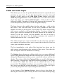
Preface
This manual is written in two parts: the first is a general introduction to
Deckman. The second section contains instructions on how to use Deckman.
Part 1: In the first chapter, a general overview of the Deckman display
screen is given with descriptions of the various parts.
Part 2: This section deals with the operation of Deckman. The first
chapters cover the installation and general use of Deckman. After
this, there are chapters dealing with specific features.
The manual includes a full Contents and Index. Since many things are referred
to in more than one place, it is advisable to check these if the information you
need is not immediately obvious.
v
Intentionally Left Blank
vi
Contents
Chapter 1 : Deckman Introduction _______ 1.1
Chapter 2 : Getting Started ____________ 2.1
Deckman Installation......................................................................2.1
Installing charts ..............................................................................2.2
Connecting to the Instruments .......................................................2.7
Direct connection of GPS...............................................................2.9
Show incoming data .......................................................................2.9
Deckman re-installation over an existing version........................2.9
Chapter 3 : Navigation ________________ 3.1
Introduction.....................................................................................3.1
Simulation .......................................................................................3.3
Selecting a route .............................................................................3.4
Quick route......................................................................................3.6
Sailing the course ...........................................................................3.7
Set DR position ...............................................................................3.9
List Route.........................................................................................3.10
What If? ...........................................................................................3.11
Planning ..........................................................................................3.14
Edit Marks.......................................................................................3.20
Tides ................................................................................................3.21
Navigation options..........................................................................3.25
vii
Display time ....................................................................................3.28
General Layers ...............................................................................3.28
Chart options ..................................................................................3.30
Chart Layers ...................................................................................3.31
Zoom ................................................................................................3.33
Special chart views .........................................................................3.34
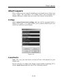
Chapter 4 : Start display ______________ 4.1
Start information.............................................................................4.2
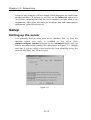
Setting the start ...............................................................................4.3
Set windward/leeward ....................................................................4.5
Start options ....................................................................................4.6
Start countdown ..............................................................................4.6
Hold wind ........................................................................................4.7
Wind calibration .............................................................................4.8
Advanced options............................................................................4.8
Chapter 5 : Data_____________________ 5.1
Time plot..........................................................................................5.1
Wind Plot.........................................................................................5.2
Data Log..........................................................................................5.4
Boat parameters..............................................................................5.8
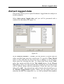
Extract logged data ........................................................................5.11
Speed Test .......................................................................................5.12
Show Data .......................................................................................5.15
Data averages .................................................................................5.20
viii
User variables.................................................................................5.20
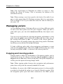
Chapter 6 : Polars____________________ 6.1
Understanding Polars ....................................................................6.1
Managing polars.............................................................................6.4
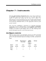
Chapter 7 : Instruments_______________ 7.1
Configure comms ............................................................................7.1
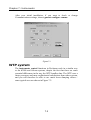
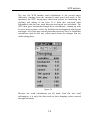
WTP system .....................................................................................7.2
h2000 Performance Unit................................................................7.7
NMEA FFD/h1000 .........................................................................7.10
Ockam Instruments .........................................................................7.11
Silva NMEA.....................................................................................7.12
NKE NMEA .....................................................................................7.13
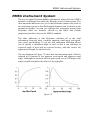
NMEA Instrument System ..............................................................7.15
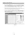
Chapter 8 : Wind calibration ___________ 8.1
Wind shear ......................................................................................8.1
Wind speed and Wind angle...........................................................8.1
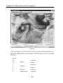
Chapter 9 : Wind and current forecasts ___ 9.1
GRIB viewer ....................................................................................9.1
Downloading GRIB forecasts ........................................................9.4
GRIB tools.......................................................................................9.8
Making wind or current Grids .......................................................9.11
GRIB routing...................................................................................9.18
ix
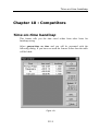
Chapter 10 : Competitors______________ 10.1
Time-on-time handicap ..................................................................10.1
Plotting competitors' positions ......................................................10.3
Chapter 11 : Networking ______________ 11.1
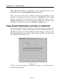
Using the networked version..........................................................11.1
Setup ................................................................................................11.2
Two-boat telemetry across a network ...........................................11.4
Chapter 12 : Deckman files ____________ 12.1
deckman.ini .....................................................................................12.1
Data files .........................................................................................12.5
j_varsXX.d.......................................................................................12.7
User variables.................................................................................12.13
Example J_varsXX file ...................................................................12.27
x
Deckman Introduction
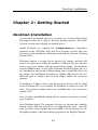
Chapter 1 : Deckman Introduction
Congratulations and thank you for choosing B&G Deckman, the world’s
most advanced race navigation software. Deckman represents B&G’s
commitment in providing software of the highest quality and
performance.
To get the most from Deckman, take the time to carefully read this user
manual so that you can fully appreciate its functionality.
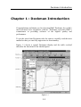
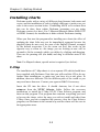
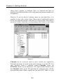
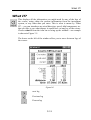
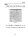
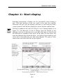
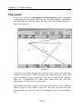
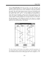
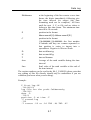
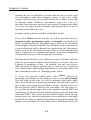
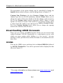
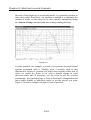
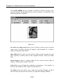
Figure 1.1 shows a typical Deckman display and the table overleaf
describes the functions of the labelled parts:
Figure 1.1
1.1
Chapter 1: Deckman Introduction
Data bar
shows the value of any variable. You can select which
variables you want displayed: simply click on the top
half of a particular box and choose from the menu. You
can display either the present or damped value (time
specified in minutes; variable is shown underlined):
choose when first selecting variables, or change by
clicking on a displayed variable and then enter the
averaging time. You can also arrange variables in the
data bar using drag and drop.
A new line of data boxes will appear when the last box
on the previous line is filled, so make sure this is left
empty if you do not want a new line of boxes.
Can be toggled on and off by selecting
menu>view>Data Bar.
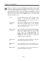
Tool bar
gives shortcuts to frequently used tools.
Icon bar
clicking on an icon will either access a display window
or provide a menu.
Status bar
bar along the bottom of the display. Shows the latitude
and longitude of the present position of the cursor and
also the range and bearing from the boat to the cursor
(right hand side).
Also provides information about the effects of some
menu choices when the cursor is held over them (left
hand side).
Can be toggled on and off by selecting
menu>view>Status Bar.
When using the program it is generally found best to have it set up with
the main Navigation window covering the majority of the display.
Behind this, but accessible, you could have things such as What If?,
Planning and a wind plot, as in Figure 1.1. That way, you can always see
your position on a chart, but are able to get to other information as and
when required.
1.2
Deckman Introduction
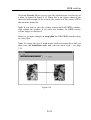
Clicking menu>refresh updates the display, thus getting rid of old or
unwanted lines or marks. If, for example, you want to view only the
isochrones from the present plan, this is a useful function.
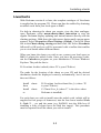
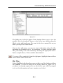
Throughout this manual, bold text is used when options—such as menu
choices—are referred to. The > symbol is used when menu selections
are being discussed. For instance, menu>zoom>from boat to mark
would mean clicking on menu on the Icon bar and then selecting the
zoom option from the pop-up menu, followed by from boat to mark—
this is illustrated in Figure 1.2. Information regarding the effect of a
particular command can be seen in the status bar.
Figure 1.2
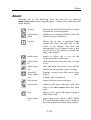
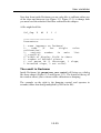
Shortcuts
The following shortcut keys are available in Deckman:
F2
Next waypoint
Sh+F2
Previous waypoint
1.3
Chapter 1: Deckman Introduction
F6
Wind plot
F7
Start display
F8
Navigation display
F9
Next window (the least recently used of all the
windows currently open in Deckman)
Sh+F9
Previous window (the most recently used of all the
windows currently open in Deckman)
Hint: using the F9 and Sh+F9 allows you to toggle between two
windows.
1.4
Deckman Installation
Chapter 2 : Getting Started
Deckman Installation
As previously mentioned, there are currently two versions of Deckman
that support either the C-Map or Euronav charting systems. The install
for each version varies slightly as detailed below.
Install Deckman by running the SetupDeckman.exe installation
program on the CD-ROM. Note that for a Euronav version, there are
two parts to the installation: Deckman itself and the Euronav Charting
System (ECS).
Deckman requires a security device known as a dongle, and this will
need to be connected to either the parallel or USB port of your computer
before you go any further. Having connected the dongle, run Deckman
from the Start button. At this point Deckman should recognize this is a
new installation and put up a dialog asking you to install the driver for
the dongle: the installation procedure is slightly different for the two
different types of dongle, but for both simply follow the on-screen
prompts.
If installing a C-Map version, then the necessary drivers will be found
on the Deckman CD so you simply tell Windows to search on your CD
drive. The Euronav dongle drivers are installed onto your hard drive
with the ECS.
Once you have installed the dongle drivers it may be necessary to restart
your computer.
Start Deckman again. The program will now go through the complete
startup routine, and then ask you for a 16-digit security code – enter the
code you have been supplied, then click OK. You should then see the
navigation window with some initial waypoints in the English Channel.
2.1
Chapter 2: Getting Started
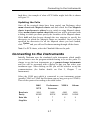
Installing charts
Deckman works with a variety of different chart formats, both raster and
vector, and the installation of each is slightly different, so make sure you
refer to the correct section below. If installing ARCS or Livecharts then
this can be done from within Deckman (assuming you are using
Deckman version 4 or later). For C-Map and Maptech charts (BSB, PCX
or REML formats) the installation is done without Deckman running.
When you first start the program after installing new charts the effect of
updating the chart folio may not be immediately apparent because the
supplied charts do not cover the area of the English Channel occupied
by the default waypoints. Use the zoom out tool: this works in the
opposite way to zoom in—the image you are looking at now will be
zoomed to fit the rectangle which you define by clicking and dragging.
Then use the panning tool (the hand) and drag to different areas of the
chart.
Note. For Maptech charts, special action is required (see below).
C-Map
The installation of C-Map charts is via a separate CD which should have
been supplied with Deckman. Note that you will need this CD to do any
further chart installations, so make sure you keep it in a safe place. In
addition, there are different CDs for different parts of the world so you
may need more than one. Contact your agent or B&G if necessary.
Insert the CD into the drive. It should Autorun, but if not select
setup.exe from the NT/PC Selector folder. Follow the on-screen
instructions to install the C-Map NT/PC Chart Selector program, and
then run this program. This program then contains everything you need
to browse the charts, select the ones you wish to install and order from
C-Map. Once you have completed the process, close the Chart Selector
program, run Deckman in the normal way and the charts will be seen in
the appropriate areas.
2.2
Installing charts
Livecharts
With Deckman version 4 or later, the complete catalogue of Livecharts
is supplied on the program CD. Charts can then be enabled by obtaining
an unlock code from your local agent or B&G.
For help in choosing the charts you require, view the chart catalogue:
open Deckman, select menu>charts>chart interaction to stop the
regular Deckman display updating and instead interact directly with the
charting package. Hold down the right mouse button until a popup menu
appears. Select Properties>Chart Settings (Global). Check the View
box in the Chart catalog viewing and then click OK. Select Livecharts
followed by OK and you will be presented with a toolbar that enables
you to view details about different charts.
When you know the charts you wish to use, contact your local agent or
B&G to obtain the unlock codes. Once you have the necessary codes,
run the Unlock.exe program on your distribution CD from Windows
Explorer. The path for this is:
D:\Livechart Archive\unlock (where 'D' is your CD drive)
The paths for the location of the charts on your CD and the desired
destination should be displayed correctly automatically, but if not set
these as follows:
Install
from
charts
D:\Livechart Archive\charts\live_b (where 'D'
is your CD drive)
Install
to
charts
C:\Charts\Live_b (where 'C' is the drive where
Deckman is installed)
For each chart you wish to install enter the unlock code (which will be
supplied in four groups of characters) into the four boxes marked Code
1, Code 2 … etc and the name (e.g. BA2045) into the fifth box (if
installing a folio of charts leave the final box empty). This procedure
must be repeated for all the charts you wish to install.
2.3
Chapter 2: Getting Started
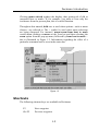
The next step is to tell the program where to find the charts. Choose
menu>charts>chart settings. A dialog will pop up giving you all of the
options for controlling the appearance of the charts. Select the Chart
Directories tab and set the directory for Livecharts - Vector by hitting
the Browse button. Move to the correct directory and then choose the
Select Path button. The path for Livecharts should be:
C:\Charts\Live_b (where 'C' is the drive where Deckman is installed; if
you specified an alternative destination for the charts in the Install
charts to box above, this should be entered here)
Note If using versions 3 or earlier, the installation for Livecharts is as
follows.
Close Deckman, enter the CD-ROM (or diskette) into the drive and
follow the installation procedure. If you are prompted for a filename
then
use
the
8
character
names
as
follows:
progra~1\BandG\deckman\charts\live_b. When you have finished,
restart Deckman and select menu>charts>update folio to update the
chart folio.
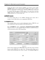
ARCS charts
Deckman needs to be running for this installation. The first task is to
install the permits: put the permits floppy disk into the disk drive then
choose menu>chart>install chart and you will be presented with a
series of dialogs which help you do the installation.
Choose Yes to install new permits
Choose Skipper permits
Install permits from disk
Choose the PRESS to Install Permits button, then Next.
Now you will be asked to insert the CD-ROM (the CHART CD-ROM
not the UPDATE). Select the PRESS to start installation button for the
install to begin. In the summary information you will see that some of
the charts require an update; after you have hit the Next button you will
2.4
Installing charts
be asked to insert the UPDATE CD-ROM. After clicking Finish you
will be asked to update the folio again.
The next step is to tell the program where to find the charts. Choose
menu>charts>chart settings. A dialog will pop up giving you all of the
options for controlling the appearance of the charts. Select the Chart
Directories tab and set the directory for HCRF - Raster by hitting the
Browse button. Move to the correct directory and then select the Select
Path button. The path for ARCS charts should be:
C:\Charts\ARCS (where 'C' is the directory where Deckman is installed)
Maptech charts
When using BSB, PCX or REML charts it is advised that these are
copied onto the hard drive of your computer. It is possible to run
Maptech charts directly from a CD-ROM, but Deckman will operate
much more quickly if the charts are read from the hard drive. If you
wish to read the Maptech charts directly from a CD, then go straight to
Updating the Folio below. In this case the path to specify will be a
folder on your CD.
If you wish to run the Maptech charts from your hard drive, copy the
charts into a folder in the top level of the drive in which you installed the
program, for instance:
Chart type
Directory (where 'C' is the drive where the program is
installed
BSB
C:\BSBChart
PCX
C:\PCX952 (see below for more information)
REML
C:\REMLChart
For BSB and REML charts simply copy the required charts into the
folder and then go to Updating the Folio below.
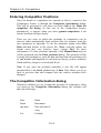
For PCX charts, the simplest thing to do is to copy the entire contents of
the CD into a folder in the top level of the drive on which Deckman is
installed. It is advised that this folder is called something like PCXnnn
(where nnn is a reference number from the particular CD: if installing
2.5
Chapter 2: Getting Started
charts from a number of different CDs, it is advised that these be
installed into different folders each with appropriate names/numbers for
recognition).
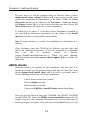
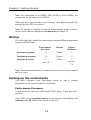
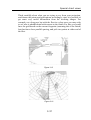
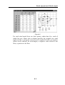
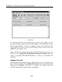
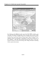
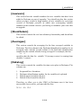
However, if you are short of memory space on your hard drive, it is
possible to copy only certain charts. This is more complicated because
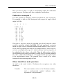
of the way Deckman interacts with the PCX chart format. Each chart is
stored in a folder which has a corresponding chart header in the folder
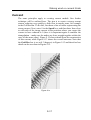
Figure 2.1
Charthdr on the CD-ROM. Both of these sections are required by
Deckman and must be stored in the same structure as on the CD. You
must therefore create a subfolder named Charthdr within the
PCXChart folder on your hard drive. The required chart headers from
the Charthdr folder on the CD must then be copied into here with the
corresponding chart folders copied into the main PCX folder on your
2.6
Connecting to the Instruments
hard drive. An example of what a PCX folder might look like is shown
in Figure 2.1.
Updating the Folio
Once all the required charts have been copied, run Deckman, select
menu>charts>use Maptech charts and then check the Use Maptech
charts in preference to others box to switch to using Maptech charts.
Select menu>charts>update chart folio and you will be presented with
a dialog in which you must specify the locations of the Maptech charts.
Click Add and then browse through the tree structure to specify the
directories in which the Maptech charts are installed. Once you have
specified the directories for all the Maptech charts you have loaded,
click Update and you will see Deckman running through all the charts.
Note. For PCX charts, select the Charthdr folder as the path.
Connecting to the Instruments
Initially Deckman uses the simulated yacht instruments which enable
you to learn to use the program without having to be on the yacht. To
change to use the boat instruments go to gmenu>change instruments
and you will be presented with a dialog so that you can select your
instrument type. After clicking on OK you will be asked to set up the
communications (for further details see Part 2, Chapter 7 on
Instruments).
Select the COM port which is connected to your instrument system
(usually COM1 or COM2 but Deckman can use any port up to COM10).
Then set the protocol according to the table below.
Baud rate
Parity
Data bits
Stop bits
B&G
WTP
Performance
Processor
NMEA
Ockam
9600
NONE
8
1
9600
EVEN
7
2
4800
NONE
8
1
4800
NONE
8
1
2.7
Chapter 2: Getting Started
Note. For connection to an NMEA FFD, h1000 or Silva NMEA, the
connections are the same as for NMEA.
When you have specified the correct settings, click Next to specify the
settings for your GPS (see below).
Note. To operate a working version in demonstration mode so that it
may be used without a dongle see deckman.ini in Chapter 12.
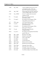
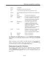
Wiring
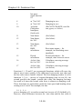
The following table details the connections between different instrument
systems and Deckman:
Performance
Processor
Ockam
9-pin to
Deckman
Instrument ground
11
7 black
5
Instrument transmit
10
3 green
2
Instrument receive
9
2 blue
3
join 4-6,
7-8
join 7-8
Note. The instrument transmit is connected to receive on your computer
and vice versa.
Setting up the instruments
You must configure your instrument system so that it outputs
information in the correct format for Deckman.
Performance Processor
You must set the system to 9600 baud, EVEN parity, 7 data bits and 2
stop bits.
On an FFD, select waypoint>cross tr on one section of the display, and
calibrate>cal val1 on the other. Set the value to 0.
2.8
Direct connection of GPS
Now select waypoint>cross tr on one section of the display, and
calibrate>cal val2 on the other. Set the value to 6.2.
Ockam
To set the Ockam RS232 interface to 4800 baud, NO parity, 8 data bits
and 1 stop bit, set both switches A and B to 9.
Direct connection of GPS
It is possible to connect your GPS directly to Deckman. The main
advantage of this is that you can easily see if you lose GPS signal for
any reason and Deckman may also receive the GPS data at a higher
frequency.
After clicking Next to setup the communications with the instruments,
you will be presented with a dialog which controls how your GPS is
connected. Select Instrument System if your GPS is connected via your
instruments or Deckman for a direct connection, followed by Finish.
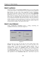
Show incoming data
After you have connected and correctly configured your instruments,
and possibly GPS (if going directly to Deckman as described above),
you may wish to check that the instrument data is being received by
Deckman. Click gmenu>show incoming data, select either Instrument
Data or GPS Data followed by Start. You should then see the data in
the window of this dialog.
Deckman re-installation over an existing
version
Note. This section should be skipped if NOT installing over an existing
version.
With Deckman running and with an instrument system connected,
choose gmenu>configure comms and make a note of the settings in the
Communications dialog. For the old style dongle (serial number
beginning 1071) you must also make a note of parameters: in Notepad
open the Deckman.ini file (see “deckman.ini” in Chapter 12) and note
the [livechart] path. Close Notepad.
2.9
Chapter 2: Getting Started
Next, you must remove the existing version. Select the Start button and
then Settings>Control Panel>Add/Remove Programs. For Euronav
versions, both Deckman Vn.n (where n.n is the version number) and
Euronav Charting System must be uninstalled.
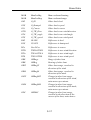
Run Windows Explorer and make copies of following files in the Data
subdirectory (see page 12.5) to somewhere other than the Deckman
directory:
Adjvt.d
wind speed calibration
adjwa.d
wind angle calibration
bgbounds.d
B&G instruments
data bounds
Bgcalib.d
Calibration
Bgdamp.d
Damping
bgout.d
Output
databar.d
Data bar settings
diamonds.d
Tidal stream data
j_nav28.d
Layers information
j_way.d
Waypoints file
Navpol.d
Navigation polar
Ockcalib.d
Ockam instruments
Calibration
Ockdamp.d
Damping
ockoptn.d
Options
ockout.d
Output
Perfpol.d
Performance polar
report.d
Reports file
shore.d
Shoreline information
Startpol.d
Start polar
Tides.d
Tidal heights data
Once all these files are backed up, delete the Deckman directory (before
doing this, it is just worth checking that no charts have been installed
here: chart directories should be as described in ‘Installing Charts’
above).
2.10
Deckman re-installation over an existing version
Install Deckman by running the SetupDeckman.exe installation
program on the CD-ROM. There will be two sections to the installation:
Deckman and the Euronav Charting System which is automatic after
Deckman.
Once installation is complete, if using an old dongle (SN beginning
1071), you must set the [livechart] path in the Deckman.ini file to that
noted above.
Copy the files you backed up above into the new Data directory,
overwriting the files that have been installed with the new installation.
The remainder of the installation is as normal (as described at the
beginning of this chapter). Run Deckman and connect to the appropriate
instrument system. Select gmenu>configure comms and set the
Communications protocol as noted in the first step.
2.11
Introduction
Chapter 3 : Navigation
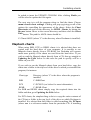
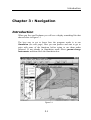
Introduction
When you first run Deckman you will see a display something like that
shown below in Figure 3.1
The best way to get to know how the program works is to run
Simulation (see next page). Here you can practice and start to get to
grips with some of the functions before trying to use them under
pressure! If not already in Simulation mode select gmenu>change
instruments and then check the Simulation box.
Figure 3.1
3.1
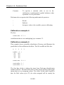
Chapter 3: Navigation
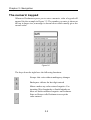
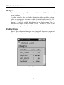
The numeric keypad
Whenever Deckman expects you to enter a numeric value a keypad will
appear like the example in Figure 3.2. The number you enter is shown at
the top in larger size; a message is shown below which usually gives the
current value.
Figure 3.2
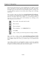
The keys down the right have the following functions:
Escape: this exits without making any changes
Backspace: deletes the last digit entered
Minus: makes any value entered negative. For
inputting West longitudes or South latitudes as
these are both considered negative on Deckman.
Enter or Return: tells Deckman to accept the
value entered
3.2
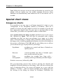
Simulation
Simulation
When Simulation is running Deckman generates instrument data that
you can use to practice running the other displays. In Simulation mode
you can only control the boat's heading and the true wind
speed/direction. Deckman then uses these to calculate boat speed and all
the other variables.
As you will not be connected to any position fixer, such as GPS, when
running in Simulation mode you will have to use Deckman's dead
reckoning (DR) capabilities to set the position of the boat. This will be
done automatically when you start the program.
When using DR, position is updated regularly according to the boat's
speed and course and the tidal information. The DR position can also be
set manually to the position of a mark or by specifying a latitude and
longitude. The most useful function (especially in Simulation mode) is
menu> waypoint>set DR>DR at waypoint to put the boat at the first
mark. See Set DR position (on page 3.9) for more details on this.
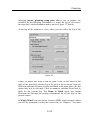
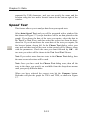
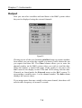
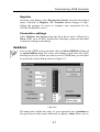
To change the boat's heading or control the wind, choose
gmenu>instruments control and you will be presented with the
following dialog:
Figure 3.3
3.3
Chapter 3: Navigation
The left pane controls the wind: click on a box to input the desired
value. If Add wind shifts is checked then Deckman will add changes in
both wind speed and direction.
On the right you can control the boat's heading: click on the box where
the present heading is displayed, (000° in the example), input the new
heading on the numeric keypad and then hit the Enter key.
After you have made the desired changes hit OK. The Data bar gives
you the option of viewing any of the variables from the database. Click
one of the boxes when highlighted with the cursor over it and select a
variable to be displayed from the list.
In some ways running Deckman Simulation mode is actually harder than
when it is being fed data by a real instrument system on board as you
have to alter the boat's heading (as described above) rather than this
being done by the helmsman. It does, though, provide an excellent way
to learn how to use the program.
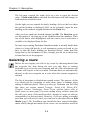
Selecting a route
Before the race begins you will set up a route by choosing marks from
the waypoint list, then during the race you only have to instruct
Deckman to go on to the next waypoint and all of the calculations will
be done with respect to the new mark. Deckman does not automatically
advance to the next waypoint on a route when the current waypoint is
reached.
The list of waypoints is divided into named sectors. The purpose of this
is to divide up the waypoints to make them easier to manage when
sailing in different places. When you first get Deckman you will find
that there are sectors named Triangle, Solent_A-M, Solent_M-Z,
Channel, Fastnet, Nioulargue, Porto Cervo, qkroute (these refer to
Quick route, see next page); if you are sailing in any of these areas this
list will cover most of the marks needed—though of course we take no
responsibility for their accuracy. However, if you are sailing in another
area then you will need to enter you own lists as described later in Edit
Marks (page 3.20). In addition you should also have entered subsidiary
marks which, though not marks of the course, are nevertheless useful as
3.4
Selecting a route
reference points on the plot—rocks and positions marking channels for
example. Sometimes it is useful to make one of these marks a mark of
the course because then you can relate laylines to that point and these
will help in making tactical decisions regarding the course to sail.
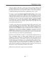
To create a route select menu>waypoints>make route or click on the
icon (shown left) on the tool bar. When you open the display you see the
names of all the waypoint areas and below a list of waypoints in the area
selected; click the arrows next to the name to move to a new sector. You
can alter the order in which the waypoints appear: clicking on sorted
will display the waypoints alphabetically, whilst unsorted will show
them in the order they were entered—useful if this is the order they will
be needed in a particular race.
To make a route click on the waypoints from the lists in the order of the
course beginning with the start mark. Those selected will then be
displayed in the Route box on the right of the window; highlight in the
Route box and click delete to remove. Also shown will be a letter P or S
indicating the direction of rounding—highlight a waypoint and click
switch rnd to change this. If the start and finish are the same you do not
need to select the finish because Deckman treats routes as circular: when
it gets to the end it goes back to the beginning again.
The first sector in the list, Triangle, is a special list: in many races you
have a triangular course, or some marks which will be set by the
committee—almost certainly a leeward mark at the start, and often an
initial windward mark—and to make it easy to set up triangular courses
Deckman has special facilities to set a wing mark and a mark half way
up the windward leg by simply specifying the range and bearing of the
windward mark from the leeward mark. In addition, the positions of
each end of the start line (see Setting the start on page 4.3) are stored in
this sector so you can use these as marks of the course.
Note. Do not remove the Triangle sector from the list.
3.5
Chapter 3: Navigation
Note. You can edit the Triangle sector and change the names (to use a
language other than English, say) but do not change the order of these
waypoints—Deckman positions all the marks for triangular courses by
using the order of waypoints.
Quick route
Selecting menu>waypoints>quick route or clicking on the icon shown
on the tool bar allows you to choose a route by setting marks using the
position of the mouse. It is also possible to include fixed marks in a
Quick Route – simply hold the cursor near an existing mark (it will turn
red) and then click the left mouse button.
Once you make the selection the cursor will be accompanied by a box
containing the range and bearing of the position of the cursor from either
the boat (if the first mark) or from the previous waypoint. The value
beside Total at the bottom of the box shows the total distance in the
present quick route.
Click the mouse at the position you wish to set each mark and then
double click at the final mark. You will then be given the following
options:
Repeat
allows you to repeat the above process
save as
marks
puts the positions of the marks you've created into
the waypoints file, where they can be edited or
used in routes as normal.
save as route
turns the quick route into the present route, in
which case it will operate as usual.
With either of the second two options, the marks will be given the
names 'q1, q2....' etc though these can be changed to something more
meaningful in the Edit Marks window (see page 3.20).
Note. While the Quick Route option is turned on, you are still able to
zoom in and out. You can, therefore, zoom in to see the position of a
mark accurately and then zoom out again to set the next mark.
3.6
Sailing the course
The Quick Route facility also allows you another way to set the
positions of waypoints (see also Sailing the Course below). Click on the
Quick Route icon, point the cursor at the waypoint you wish to move (it
will turn red). Hold down the left mouse button and drag to the required
position. If you are moving a quick waypoint (q1, q2 etc), then the
waypoint will be moved; if you try to move a fixed mark, then a new
waypoint will be created in the position you drag to with a Quick Route
name.
You are also able to add or remove waypoints from the current route
using the Quick Route facility. To add a waypoint to the current route,
select the Quick Route icon and then point the cursor at the waypoint
after which you want to add the new mark (it will turn red). Without
clicking the mouse button, move the cursor to where you want the new
waypoint and double click, followed by save as route. To remove a
waypoint, select the Quick Route icon and then highlight the waypoint
you wish to remove from the route (it will turn red). Hold down the left
mouse button and drag the waypoint to either the previous or next
waypoint, release the mouse button.
Sailing the course
All of the above preparation should ideally happen before the race
begins; during the race you then just instruct Deckman to go to the next
waypoint and all calculations will be done with respect to the new mark
(the name of the present leg is shown in the box at the top of the
display):
(F2)
(Shift F2)
next waypoint—clicking on this means all
calculations are made with respect to the
next waypoint.
previous waypoint—all calculations are
made with respect to the previous
waypoint.
3.7
Chapter 3: Navigation
There are, however, ways of changing the position of the current
waypoint to make it fit in with your observations once you start racing.
Choosing menu>waypoints>set waypoint—or by clicking on the icon
shown left on the tool bar—gives you a number of methods to set/adjust
the position of the current waypoint (usually, these would only be used
with the movable marks in the triangle sector, as the fixed marks
shouldn't normally move!):
to boat
sets the position of the current waypoint to the
position of the boat. For example, when
rounding a particular mark for the first time or
to set the start mark.
drag current
waypoint
allows you to highlight and then click-and-drag
and current waypoint only to a new position.
Once you release the mouse button, you will be
asked to confirm the move.
Ww/Lw from
windward
sets the position of the leeward mark and finish
line by range and bearing from the windward;
brings up a dialog exactly the same as that
shown under Set windward/leeward (see
Setting the start on page 4.3) except the
bearing you set in the top box is from the
windward to the leeward mark.
triangle from
lee
you position the windward mark by entering a
range and bearing from the leeward.
RB from prev
WP
set the position of the current waypoint as a
range and bearing relative to the previous mark.
RB from boat
set the position of the current waypoint as a
range and bearing from the boat.
3.8
Set DR position
Laser RB
from boat
as above. For use with a laser range finder.
triangle from
mid
set the position of the current waypoint as a
range and bearing relative to the mid mark
by lat, long
allows you to specify a latitude and longitude
Make sure that the waypoint you wish to position is the one currently
selected—its name should be at the top of the navigation display. If used
to set the windward and leeward marks in a triangular course then not
only will the positions of these be changed, but the gybe and mid marks
will also be set.
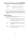
Set DR position
Choosing menu>waypoints>set DR position allows you to set your
dead reckoning position by one of three methods:
DR at WP
sets DR position to the position of the current
waypoint. This is particularly useful in Simulation
mode when, having set up a course, you can put the
boat at the position of the first mark.
DR at
GPS
puts the dead reckoning position to the current GPS
position. Especially useful to set a DR immediately
if the GPS fails.
DR by
lat, long
allows you to input your own dead reckoning
position. This will generally only be used if running
Deckman after a GPS failure.
3.9
Chapter 3: Navigation
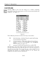
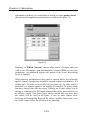
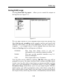
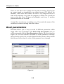
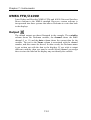
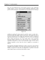
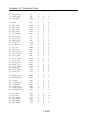
List Route
Clicking route on the icon bar brings up a window containing
information about the current route, as well as your present latitude and
longitude—see Figure 3.4.
Figure 3.4
Three different positions are shown at the top of the window:
DR
dead reckoning—calculated from the speed and bearing
received from the instruments
EP
estimated position—DR position adjusted for whichever
current is selected in Use Current in the Navigation
options window (see page 3.21).
PF
position as read from the position fixer, usually GPS.
Beneath this is a list of the marks showing on the first line of each entry
the range and bearing from either the boat if it is the first waypoint, or
from the previous mark. The second line has a letter (either P or S)
indicating the direction of rounding, followed by the latitude and
longitude of the mark from the waypoint file.
3.10
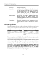
What If?
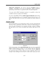
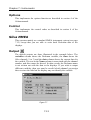
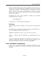
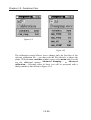
What If?
This displays all the information you might need for any of the legs of
the course, using either the present information from the instrument
system, or any other data you enter. This is what is meant by ‘What
If?’—you can introduce any wind direction, speed, tidal component, etc.
that you like to see what impact it would have on any leg of the course.
Choose what if from the icon bar to bring up the window—an example
is shown in Figure 3.5.
The boxes on the left of the window allow you to move between legs of
the course:
Figure 3.5
next leg
Previous leg
Present leg
3.11
Chapter 3: Navigation
There are three rows of boxes to allow you to control the information
used in the What If? calculations (values in the example in brackets):
C to make
grnd wind
current
Course to make to the mark
Left
Distance to the mark (2.40)
Middle
Bearing to the mark (255°)
Right
Automatic update or fixed (A)
Ground wind
Left
Ground wind speed (19.4)
Middle
Ground wind direction (74°)
Right
Automatic update or fixed (A)
Water current flow
Left
Water current speed (1.2)
Middle
Water current direction (260)
Right
Automatic update or fixed (F)
Click on any box to input a value you wish to try. The right hand
column of boxes read either F or A and show whether the value has been
fixed (F) by your entering a value or is being automatically updated (A)
by the instruments. Initially, all will read A but will switch to F if a
value is entered. Clicking on the A/F box allows you to switch between
your values and those from the instruments.
Note. Any changes made here affect only the What If? function; they do
not affect the Navigation display.
The bottom part of the display contains the calculated leg information
for each tack, or for one tack if it is a free leg:
C to sail
Course to Sail: the course to sail for the indicated leg
of the race, allowing for the current. If the leg is not a
free leg then optimum or target values are used to
calculate the courses for each tack or gybe.
Track
direction of the track which the boat makes over the
ground if sailed on the above course.
3.12
What If?
Est VS
Estimated Boat Speed; this is a speed through the
water.
AS
Estimated Apparent Wind Speed.
AA
Estimated Apparent Wind Angle.
TS
Estimated True Wind Speed.
TA
Estimated True Wind Angle.
Dist
Distance to the laylines if the leg is not free; else
blank.
Time
Time to the mark, or to the laylines if the leg is not
free.
3.13
Chapter 3: Navigation
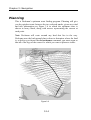
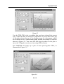
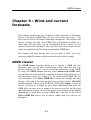
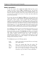
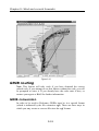
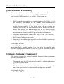
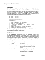
Planning
This is Deckman’s optimum route finding program. Planning will give
you the quickest route between the two selected marks, given any wind
and tide information–see Figure 3.6 in which the optimum route is
shown in heavy black, along with arrows representing the current at
each point.
Note. Deckman will route around any land that lies in the way.
Deckman uses the background chart colour to determine where the land
is, so before you choose the do isochrones command, you must zoom so
that all of the legs of the course for which you want to plan are visible.
Figure 3.6
3.14
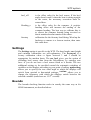
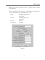
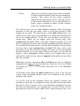
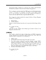
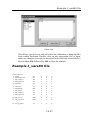
Planning
Selecting menu> planning>setup plan allows you to prepare the
variables for the Planning calculation, i.e. select the leg of the course,
the start time, wind information and so on (see Figure 3.7 below).
At the top of the window is a box where you can select the leg of the
Figure 3.7
course on which you wish to run the plan—click on the arrow to the
right of the presently selected leg to be given a list to choose from (as
Deckman assumes all routes to start and finish in the same place, the last
option may not be relevant). Click on reset to calculate from boat to
mark for the present leg. The Route to finish check box makes
Deckman run through the routing calculations for all the legs of the
present course.
In Which Wind? you can choose between GRIB wind forecasts (where
you will be prompted to select the correct file; see Chapter 11 for more
3.15
Chapter 3: Navigation
information on these) or a wind table in which you must predict wind—
direction and strength at particular times, as shown in Figure 3.8.
Figure 3.8
Similarly, in Which Current? choose what source of current data you
wish to use: Deckman's own tidal database, current GRIBs or your own
predictions. An additional option will appear if the Local Knowledge
server is enabled.
When entering information in the wind or current tables, the following
applies: times of predictions should be entered in hours and minutes. If a
prediction is 24 hours or more after the previous one, the time must be
preceded by a number equal to the number of complete 24 hour periods
that have passed since the last entry. Clicking on a value allows you to
change it; clicking in the left hand column followed by insert allows you
to add new entries. Note that if these tables contain only one entry then
the values will be used at all times; if two or more entries exist,
Deckman will interpolate between the values, and the times must cover
the whole range of time for which you are planning.
3.16
Planning
Note If using Deckman tidal database this then please see Tides on page
3.21). If using GRIB forecasts, please see Part 2, Chapter 9.
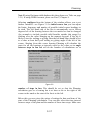
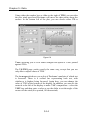
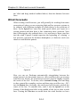
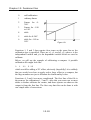
Selecting configure from the bottom of the window allows you to set
further variables—see Figure 3.9. In initial course fan you can adjust
the limits, frequency and number of possible initial course headings to
be tried. The left hand side of the fan is automatically set to fifteen
degrees left of the bearing between the two marks but can be changed
(for example to include possible tidal benefits outside this range) by
clicking over the value bringing up the numeric keypad. If the leg is
likely to involve tacking or gybing, then the left hand edge should be set
to a value at least half your tacking or gybing angle to the left of the
course. Starting from this course bearing Planning will calculate the
route for all the bearings at intervals equal to the value set in angle
between steps in fan and will do the number of calculations set in
Figure 3.9
number of steps in fan. This should be set so that the Planning
calculation goes to a bearing that is at least as far to the right of the
course to the mark as the start of the fan is to the left.
Below this you are given the option of setting the date and time of the
start of the Planning calculations. You can also select the time interval
between steps of the plan and the number of these time steps. Make sure
3.17
Chapter 3: Navigation
that the time interval between steps multiplied by the number of steps
gives a time that is at least what you expect the leg to take. Obviously,
for longer races the time between steps should be greater; trying to see
too many different options at once merely makes things more confusing,
not less so!
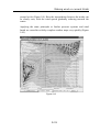
Once you have setup your plan choose menu>planning>do isochrones.
You will then see Deckman draw all possible routes, with the optimum
shown in red (heavy black line in Figure 3.6). You can then choose to
view any or all of wind, current and isochrones by clicking on the
following icons on the tool bar.
Show wind—lines point into the wind
Show current
Show isochrones
Show animation— see Animation below
edit GRIBs
setup—returns you to the Setup menu to change variables
Once you have a plan in place menu>planning>optimum details
allows you to view conditions at each time interval during the leg (note
that the time column here shows you both the day of the month and the
time).
Any number of plans can, and should, be tried to see how the optimum
route would change in various different conditions. Then a decision can
be made as to the most likely and a route chosen to match.
3.18
Planning
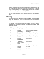
Animation
Clicking the animation icon on the tool bar allows you to move along
the route and view how the wind or current will change with time. In
Figure 3.10, you can see that in the bottom left corner, the date and time
the display is illustrating can be seen. The two buttons to the right of this
Figure 3.10
give you the option of viewing either current or wind (usual symbols,
see above). Three further buttons allow you a choice of what types of
vectors are used: always the arrows point in the direction of flow. For
the two arrows (left and middle), the size of the tip is proportional to the
speed; for the feathered pointers the number of feathers indicates the
rate—for wind one is equivalent to five knots, for tide one equals 1 knot.
For each, half feathers represent half the value.
3.19
Chapter 3: Navigation
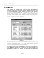
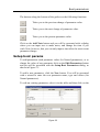
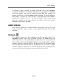
Edit Marks
The facilities for entering new waypoint sectors and waypoints
described in this section are general purpose facilities intended for race
or passage preparation. To make changes or additions to the waypoint
list choose menu>waypoints>edit waypoints; you will see the Edit
Marks window appear, as shown in Figure 3.11. The commands in the
top right of this window are for editing waypoint areas; those at the
bottom left refer to the actual waypoints.
Figure 3.11
To change the name of an area choose rename when it is selected; you
will then be prompted to enter a new sector name. Similarly, to add a
new sector choose new and then enter the name.
If you have used the quick route method to create a set of waypoints you
may rename the qkroute area to your own area name. Deckman will
automatically create a new qkroute area next time the quick route
facility is used.
3.20
Tides
To edit a waypoint—either name, short name, latitude or longitude—
simply click in the box where you wish to make the change and then use
the computer's keyboard. To enter a new waypoint click in the left hand
column (the cursor will change to an arrow) on the row where you want
to insert the new waypoint and then click new from the bottom left of
the window. A new waypoint with the name 't' will be created; edit name
or position as above. Names and positions can also be cut and pasted in
the same way.
Note. Positions are in the form: degrees, minutes and decimals of
minutes. As always, positive values are North and East; negative are
South and West.
Tides
To use the tidal facility in an area that Deckman’s tidal information
covers, you have to enter the high water times and heights for the ports
near to the area you are sailing in.
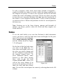
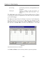
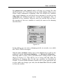
Select menu>planning>edit HW
and the dialog shown in Figure
3.12 will appear.
Put the date of the first high water
you enter in the date box. To
enter times and heights click over
the value you wish to change and
use the computer's keyboard (not
the numeric keypad here). To
insert additional entries, either
between or after those already
there, click in the left hand
column (headed HW , where you
will see the cursor change to an
Figure 3.12
arrow) at the position you wish to
make the entry and then choose
new. You can also cut and paste the entries by selecting them in the LH
column.
3.21
Chapter 3: Navigation
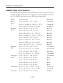
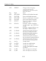
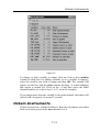
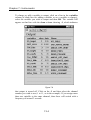
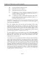
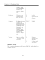
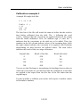
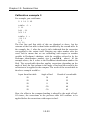
SHOM tidal information
The SHOM data is split into nine different areas; you will need to obtain
the relevant files and release codes from your agent or B&G Ltd before
use. The SHOM areas and relevant HW ports are as follows:
Name
Areas covered
HW ports
BaieDe
Seine
49 29 - 49 48 N / 1 46 - 1 03W
Cherbourg
49 38.5 – 49 40.8 N / 1 41.25 - 1 34 W
Cherbourg
49 16 - 49 47.7 N / 0 19 W - 0 14 E
Le Havre
48 36 - 49 09 N / 4 20 - 3 03 W
Roscoff
48 35 - 48 58 N / 3 44 - 3 21 W
Roscoff
48 48 - 48 51.5 N / 3 29 - 3 22.5 W
Roscoff
48 45.7 - 48 46.6 N / 3 36.4 - 3 34.5 W
Roscoff
48 37 - 48 46 N / 3 59 - 3 50 W
Roscoff
48 42.5 - 48 46.5 N / 4 05 - 3 56 W
Roscoff
48 43.4 - 48 43.9 N / 3 59 - 3 58 W
Roscoff
48 43 - 48 43.6 N / 3 58.1 - 3 57.01 W
Roscoff
46 43 - 47 52 N / 4 30 - 1 53 W
Concarneau
47 15 - 47 34.5 N / 3 21 - 2 38 W
Port Navalo
47 31 - 47 46 N / 3 36 - 3 18 W
Port Tudy
47 38 - 47 54.2 N / 4 11 - 3 49 W
Concarneau
Gascogne
42 49 - 48 30 N / 7 30 - 0 45 W
Concarneau
Iroise
47 45 - 48 46 N / 5 18 - 4 16 W
Brest
48 16 - 48 34 N / 5 09 - 4 38 W
Brest
48 00 - 48 50 N / 4 53 - 4 39 W
Brest
48 16 - 48 24 N / 4 39 - 4 14 W
Brest
48 00 - 51 53 N / 7 00 W - 3 00 E
Cherbourg
49 14 - 50 10.7 N / 1 45 W - 0 24 E
Cherbourg
48 30 - 50 18 N / 3 10 - 1 20 W
St Malo
Bretagne
Nord
Bretagne
Sud
LaManche
Normand
3.22
Tides
Breton
PasDeCala
is
Vendee
Gironde
49 32 - 49 47 N / 2 20.14 - 1 44 W
St Malo
49 21 - 49 30.4 N / 2 34 - 2 14.12 W
St Malo
49 05 - 49 14 N / 2 13 - 1 54 W
St Malo
48 47 - 49 28.5 N / 2 01 - 1 32 W
St Malo
48 37.2 - 48 45.2 N / 2 19.5 - 1 45 W
St Malo
48 31.4 - 48 42 N / 2 51 - 2 25.3 W
St Malo
48 45.5 - 49 06.5 N / 3 06 - 2 46.3 W
Paimpol
50 37 - 51 12 N / 1 00 - 2 25 E
Calais
50 43 - 50 49 N / 1 29 - 1 40 E
Calais
50 56 - 51 01 N / 1 43 - 1 54 E
Calais
51 01 - 51 06 N / 2 05 - 2 26 E
Calais
45 15 - 47 20 N / 3 00 - 1 00 W
Les Sables
d'Olonne
45 25 - 46 26.74 N / 1 42 - 1 02 W
La Rochelle
46 04.73 - 46 10.8 N/ 1 19.21 - 1 06.4W
La Rochelle
46 52 - 47 20 N / 2 52.67 - 1 58 W
Saint
Nazaire
45 25 - 45 45 N / 1 38 - 1 00 W
Pointe De
Grave
Ensuring Deckman is not running, place the relevant file in c:\program
files\BandG\deckman\data
directory
(where
c:\program
files\BandG\deckman\) is where you installed the program. The file will
be called SHOM followed by the name of the area. Start Deckman and
you will be prompted for a 16-digit code.
You can then use the data for the SHOM areas which you have enabled
in your planning calculations and so on by entering the times and
heights of high water for the relevant ports.
3.23
Chapter 3: Navigation
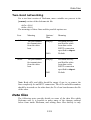
Tidal currents layer
This allows you to view the predicted tidal currents for a particular area
and time on your chart. To use this function, first enter the times and
heights of high water in the Edit High Water dialog; now click
menu>layers>general then click the Dn button to scroll to the bottom
of the list where you will find tidal currents – click on this to select
followed by OK. A number of buttons will appear at the bottom of the
screen and possibly some arrows on the navigation display.
The large button in the middle shows the date and time – click in this
and enter a new date and time (in the form yymmdd for date and
hhmmss for time) on the keypad. You will now see arrows representing
tidal current overlaid on the navigation display. You have a choice of
arrow types, which is controlled by the three buttons on the bottom left
corner. For the two arrows (left and middle), the size of the tip is
proportional to the speed; for the feathered pointers the number of
feathers indicates the rate— one equals 1 knot.
This tidal currents layer can be animated from the start time, and there
are a number of buttons to allow you to control this to the left of the box
where you entered the start time.
The box immediately to the right of the date/time box shows you the
tidal current rate/direction at the position of the cursor. Note that this
does not operate when the animation is running.
The Options button brings up a dialog which gives you some additional
controls and information about the tidal currents layer. At the top of this
dialog, the Choose button allows you to control the colours used on the
display. The colours defined in Custom Colors are used by Deckman to
show changes in current rate, with each colour representing 0.5 of a knot
of current. The Scale box allows you to control the size of the
arrows/tufts. The density box allows you control how many arrows you
have across your display in each direction (i.e. entering 20 here will give
you a 20 by 20 grid of arrow representing the tidal current).
At the bottom of the Options dialogue there is also a drop down list
showing the reference ports used by the area of the chart currently being
3.24
Navigation options
displayed. This is an easy way to check you have entered tidal
information for all the reference ports you might need.
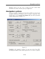
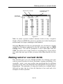
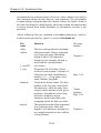
Navigation options
You have a number of options as to the sources of data you use for your
navigation functions in Deckman, such as variation, current/tide, boat
position and so on. Hit menu>view>options and you will be presented
with the dialog shown in Figure 3.13.
Figure 3.13
Variation is the magnetic variation for your area in the form dd.d.
Preceding the number with a minus sign will set it to West, a positive
3.25
Chapter 3: Navigation
number is variation to the East. Deckman will automatically calculate
variation based on your time and position based upon the world
magnetic model so you should never really need to change this.
Bearings can be set to TRUE or MAGNETIC so that all bearings,
laylines etc are displayed accordingly. This can be extremely useful in
areas of the globe where variation changes rapidly such as the Southern
Ocean.
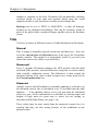
Tide
You have a choice of different sources of tidal information in Deckman:
Manual
This is simply a manually entered current rate and direction – these are
set in the current rate and direction boxes at the top of the Navigation
options window. This might be a particularly useful if you have just
noticed the current on a buoy as you sailed by.
Measured
Every 2 seconds, Deckman compares the GPS position with the dead
reckoned (DR) position, with the difference being due to current effects
(and, possibly, calibration errors). The difference is then termed the
measured current. This value is then averaged over a time period set in
the Current update time box.
Diamond
Another current which Deckman is constantly updating is referred to as
the diamond current: this is calculated every 10 seconds from the tidal
database — if the database doesn't cover your area then the calculated
values are zero. All the information is controlled by entering times and
heights of high water for ports near to where you are sailing, as
described in Edit High Water (see page 3.14).
These values may be more steady than the measured current, but it is
possible that they are also wrong because of the conditions at any
particular time.
3.26
Navigation options
Deckman has the possibility of using tidal information from SHOM, the
French Hydrographic office. For this you require additional files and
release codes.
If you have the SHOM files, then it is possible that Deckman will have
to choose between this and its own database. This is done on the basis of
the area covered by the tidal chart with smaller areas preferred as they
are assumed to be more accurate.
One thing you need to be aware of if using the SHOM files is that
Deckman makes the selection described above regardless of whether
there are any high water times entered meaning that, if no HW times are
entered for the smallest area at a particular location, then no tidal
information will be seen for this area (it will always show 0 for both rate
and direction). You must therefore either ensure that HW times are fully
entered or you can remove the files – please see Tide files on page 12.7.
If neither of these sources of tidal data cover your patch then B&G can
create a personal database if you have the necessary information.
LKCS
The Local Knowledge Current Server covers particular areas, mainly in
North America.
Position
The Use Position option gives you a choice of the source of the yacht’s
present latitude and longitude which is used in all the navigational
calculations.
dead rk
actually uses the estimated position, which is the
dead reckoning position adjusted for current.
GPS
position fixer—usually GPS.
When you switch between Simulation mode and normal use, this will
automatically toggle between dead reckoning and GPS. The only time
you should have to change the setting here is if your GPS fails, in which
case you will want to switch to using Deckman in dead reckoning mode.
3.27
Chapter 3: Navigation
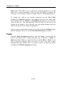
Display options
The following affect only the look of the Navigation window:
Vector scale
adjusts the length of the wind vectors
Vector gap
sets the gap between the tufts of wind vectors so
that you can see them more clearly.
If your boat does not appear to be in the right position on the chart,
entering a GPS offset here (in minutes and decimal minutes) should
help. A positive value will offset North or East; negative moves position
South or West.
Grid layer spacing allows you to set the distance between lines on an
overlaid grid. Grid layer type gives you the following options:
great circles
a great circle is drawn from your present
position to the mark, along with lines parallel
and perpendicular to this in great circle
terms.
Latitude circles
grid lines follow latitude in one direction,
with equidistant points along these connected
in the other direction
Display time
Choosing menu>view>display time allows you to set the track time,
e.g. if set to 15 minutes the boat's track (and associated information) is
displayed for the previous 15 minutes.
General Layers
Choosing menu>layers>general allows you to determine what
information is displayed on the screen. Any of the following can be
selected:
mark laylines
shows the laylines from the selected mark
boat laylines
displays the yacht's present laylines varying
3.28
General Layers
with wind, tide and tacking angle.
shoreline
Deckman can provide a simple shoreline if chart
coverage for a particular area is poor.
digital chart
allows you to see present position against a
chart—almost always left on.
North
displays a north arrow in the top left hand
corner of the screen.
Wind
shows a tuft of wind arrows at intervals along
the boat's track. The direction of the arrows
indicates the true wind direction and their
lengths indicate true wind speed. Note that the
lines point into the wind.
DR track
shows the track of the boat calculated from
Dead Reckoning, not including the current.
PF track
shows the track of the boat given by the position
fixing system, usually GPS.
Course marks
displays the waypoints that are a part of the
course that fall within the geographical
boundaries of the window.
other marks
displays in the window every mark in the
waypoint file that comes within the
geographical boundaries of the window’s
display.
GRIB view
ignore this setting (it should remain turned on).
Please see page 9.1 for details of operation of
the GRIB viewer feature.
boat
shows the present position of the boat.
join
waypoints
connects waypoints for present route by a great
circle
isochrones
gives you the option of having the toolbar icons
for Planning displayed at the top of the
Navigation screen. Most useful if left on, but
turn off to remove isochrones when you have
finished using Planning.
3.29
Chapter 3: Navigation
grid layers
displays grid layers.
course line
two lines will be displayed when this is turned
on: the solid line shows the course over ground
as read from the GPS; the dashed line is the
course through the water (i.e. heading plus
leeway, without the effects of current).
limits laylines
lets you see the extent of variation in the mark
laylines for the last fifteen minutes. The
appearance and time interval can be changed as
per page 12.6
Competitors
shows the positions of your competitors, if this
feature has been setup as described in Chapter
10.
Chart options
Though Deckman will work with a wide range of both raster and vector
charts, you are only able to select from one of the following columns:
C-MAP
Version
C-Map
vector
charts
Maptech (BSB), PCX, Reml raster
charts
Euronav
Version
Livechart
vector
charts
ARCS
raster
charts
Maptech (BSB), PCX, Reml raster
charts
These two options work slightly differently in Deckman, so please make
sure you refer to the correct section below.
The Deckman display will normally switch between the different loaded
charts automatically depending on the scale and the extent to which you
are zoomed in. However, you may wish to override this automatic
switching and are able to specify Maptech charts to be used in
preference to others. Select menu>charts>use Maptech charts and
then check the Use Maptech charts in preference to others. To turn
this feature off again, repeat the above and clear the box. The Show
Maptech chart outlines function allows you to view the positions of the
loaded Maptech charts without actually using them.
3.30
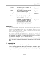
Chart Layers
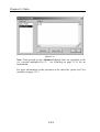
Chart Layers
This is where you can control which layers are turned on or off on your
vector charts. The procedures for C-Map charts and Livecharts are
slightly different, so make sure you refer to the correct section below.
C-Map
Select menu>charts>chart settings and you will be presented with a
dialog (see Figure 3.14) which allows you to choose which layers you
wish to see shown on your display.
Figure 3.14
Livecharts
Note. The way you turn layers on and off here will depend on your
dongle type.
For an old style, Livechart-only dongle (serial number beginning 1071)
choose menu>layers and then one of the following options:
3.31
Chapter 3: Navigation
Hydrographic
shows a dialog with standard hydrographic
layers. Once selected, these remain selected
across all the Livecharts as the charts scale and
positions change.
Livechart
shows all of the layers which are available on
the currently loaded Livechart. The layers will
vary from chart to chart. Select layers here for
fine control of layer visibility for a particular
chart.
With the new style dongle (S/N beginning 2071), all chart layers are
turned on or off by choosing menu>charts>chart settings. Layers
selected here apply across all charts.
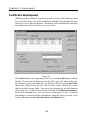
The menu>charts>colour option gives you additional controls over the
appearance of you charts.
Chart interaction
Note. This function applies only to the new style dongle (serial number
beginning 2071). Chart interaction works by turning off the Deckman
navigational layers and giving you access to the additional features of
the charting kit. It is best used by turning it on for a specific reason (for
example to select a particular chart to use) and then turned straight off
again.
Click menu>charts>chart interaction to turn on this feature which
gives you additional controls over your charts. If you now select
menu>charts you will see the option select chart. Choosing this will
present you with a 'tree list' allowing you to select any installed chart to
view. With chart interaction turned on you can use the left mouse button
to zoom in on a particular chart (by clicking in the coloured box
outlining it) or zoom out by a scale factor using the right mouse button.
For further information on
gmenu>Help>Chart System Help.
the
3.32
functions
here
choose
Zoom
Zoom
Selecting any of the following from the icon bar—or choosing
menu>zoom and then the required option— allows you to alter the scale
of the display:
this leg
displays the whole leg from the previous
waypoint to current waypoint.
from boat to
mark
displays the remaining distance from the
yacht’s position to the buoy.
on boat
allows you to view a specified range
around the boat with the boat in the
centre of the display. The boat will
automatically be re-centred when it has
moved 20% of the distance towards the
edge of the display.
whole route
zooms to allow you to see all the
waypoints in the current route
Chart zoom
in
click and drag to select the area to zoom
in on.
Chart zoom
out
click and drag: the present view will be
shrunk into the position of the rectangle.
zoom full
chart/ zoom
out
Euronav: zooms to the full extent of the
loaded
chart.
C-Map: click to zoom out.
Last zoom
zooms to the previous scale/area
Next zoom
zooms to the next scale/area; will only
work if the last zoom button has been
used.
Pan
allows you to 'move' the chart keeping it
at the same scale.
Chart zoom
1:1
when using raster charts (ARCS, BSB,
PCX) this function allows you to zoom to
the scale at which the chart was scanned.
3.33
Chapter 3: Navigation
Note. Whilst the zoom in, zoom out and pan functions are turned on, the
display will not update (e.g. the yacht's position). However, these
functions will automatically turn themselves off if left inactive for 15
seconds.
Special chart views
Images as charts
It is possible to use any .jpg or .gif image instead of a chart as your
‘background’ in the Navigation window of Deckman. There are a
number of reasons why this might be useful, for example if you do not
have appropriate digital charts for your area or, and especially in long
ocean races, you wish to use specialist weather or tidal charts.
Select menu>charts>use image as chart and then browse to the correct
file, followed by Open. You will then be presented with a dialog
reminding you that you must geo-reference your image up to three
times. Geo-referencing is simply telling Deckman which positions on
the image refer to which geographical positions; see below for details on
the process in Deckman. Click OK and the next dialog you see allows
you to choose the type of projection of your image:
Equidistant
meridians are vertical and lines of latitude are
equally spaced
Mercator
vertical meridians but lines of latitude space
more widely towards the poles
Polar
stereographic
meridians are straight lines from poles –
usually used for geostationary satellite images
Pick the correct one, followed by OK.
The geo-referencing process then involves entering the latitude and
longitude of known positions on the image. After you have selected the
type of projection above, the cursor will appear as a cross with the
number ‘1’ beside it – click at a known position on the image and enter
the lat/long in the dialog (as always in Deckman, North/East are
3.34
Special chart views
positive, South/West as negative) followed by OK. The number beside
the cursor changes to a ‘2’ and you repeat the above process (possibly
twice more).
Note. You are still able to use the zoom in/out tools to increase
accuracy.
Once you have completed geo-referencing (a dialog will pop up telling
you when this is the case), Deckman operates as normal, except that the
only ‘chart’ you use is the image you have chosen.
To exit this feature and return to normal charting,
menu>charts>use image as chart followed by Cancel.
select
Warp image
This function allows you to manipulate your chart so that a great circle
route is changed from being curved (as usual in Deckman) to being a
straight line. This is particularly useful in a long race (and especially
with the ‘Competitors’ feature – see page Chapter 10), as it allows you
to get a proper idea of who is ahead/behind with respect to a certain
waypoint or the finish.
For example, you could convert the image shown in Figure 6.15 to that
in Figure 6.16, in which the great circle route from Land’s End to New
York is shown straight.
Select menu>chart>warp image and you will be presented with a
dialog reminding you how this feature operates; click OK. You must
then select two points on the display – the first will be shown at the top
of the screen and is the centre of the projection while the second will be
shown directly below it. Before you select the points, hit the grid
options button (shown left) at the top of the display to choose what grid
lines and spacing you want to have displayed on the warped image: you
can choose to have the grid centred on different points with different
meridian and parallel spacing:
Off
No grid
North pole
Grid based on the North pole; will be the
same as normal lat/long grid
3.35
Chapter 3: Navigation
Current waypoint
Meridians from the current waypoint, parallel
lines at equal distance from the current
waypoint.
Projected centre
Meridians from the projection centre (the
first point you select), parallel lines at equal
distance from the projection.
Note. The spacing units are in degrees and decimals (ddd.dd).
Hint. For meridian spacing, something like 20° is usually appropriate,
since this gives you 18 meridians 20° apart. The parallel spacing
depends very much on how far apart the two points you choose are – see
below.
You then pick two points and the image is warped so that the great circle
route between the two points is represented as straight and the chart is
altered to accommodate this. You cannot zoom out beyond what is
shown on the chart at the time you select warp image so make sure both
points you wish to select are visible. You can zoom in to position them,
however.
3.36
Special chart views
Think carefully about what you are trying to see from your projection,
and choose the points and grid options accordingly, since it is possible to
get some very useful information from the resulting images. For
example, on a long race but with the fleet in a close area you may wish
to see who is ahead/behind with respect to the finish. For this you would
have the grid based on the current waypoint (assuming this is the finish)
but then have close parallel spacing, and pick two points at either end of
the fleet.
Figure 3.15
Figure 3.16
3.37
Special chart views
Chapter 4 : Start display
Deckman incorporates a display for use specifically when starting a
race. With the position of the two ends of the start line entered,
Deckman will give you the distance and time to each from the boat's
current position, and will also display the current laylines and line bias.
Clicking on start on the icon bar will give you a starting display as in
Figure 4.1; the direction of start is always from the bottom of the
diagram to the top, so that the port or pin end of the line is to the left and
the starboard or committee boat end is on the right. The line above the
start line indicates the present line bias—it is drawn from whichever end
of the line is favoured, the port end in the diagram. The pairs of lines
drawn from each end of the line are the laylines.
Figure 4.1
4.1
Chapter 4: Start display
Start information
The Start display contains a Data bar similar to that in the main
Navigation where you can view any data variables you choose. When
the Start display is open, select menu>Databar to toggle this on or off.
This data bar then operates in exactly the same way as the Navigation
data bar (see page 1.1 for details).
At the top of the display in the centre are two numbers: the one on top
shows the perpendicular distance from the bow to the line (in the
presently selected units, metres or boat lengths, see below) whilst
underneath is shown the countdown to the start. The other numbers at
the top of the display show (from left to right) distance and time: to the
port end of the line, to the intersection of the start line with a starboard
tack layline drawn from the boat's present position, to the intersection of
the start line with a port tack layline drawn from the boat and to the
starboard end of the line.
The figures at the bottom of the display show the following:
LL
Bearing down the left layline, adjusted for current
LineWD
line wind direction, i.e. the wind direction required
for the line to be neutral
BiasG
the distance in the presently selected units (see
below) which the line bias is worth
BiasA
the angle of line bias, along with the favoured side (P
or S)
LR
Bearing down the right layline, adjusted for current
Distances (D) can be given either in metres (in which case an 'm' will be
shown after the D, as in the diagram) or boatlengths (which must be set,
see Start options on page 4.6). To switch between the two, choose
menu>toggle units. There are also two possible ways of viewing the
time: if a 'B' follows the 'T' then the times are presented as "time to
burn", i.e. the difference between the time remaining and the time it will
take to cross the line. Obviously, this will only be displayed if the
countdown has started. Choose menu>toggle time to change between
these time formats.
Note. ‘Time to burn’ will appear as negative if you are late for the start!
4.2
Setting the start
Setting the start
Clicking on menu allows you to set the position of the line:
Set port end
(see below)
Set port + lee
sets the port end of the line and the
leeward mark to the position of the boat
Set starboard end
(see below)
laser port end
sets the port end of the line using a laser
range finder
laser port + lee
sets the port end of the line and the
leeward mark using a laser range finder
laser starboard end
sets the starboard end of the line using a
laser range finder
Set windward/leeward
(see below)
Set port/starboard
When you select either set port or set starboard you will be given a
choice of the following (note that the text assumes you are setting the
position of the port end for ease of reading)
PING port
move the buoy to the position of the bow of
the boat.
nudge (+upwind,
–downwind)
move the buoy a distance specified in
metres either upwind (a positive number) or
downwind (a negative number). The
direction of movement is at right angles to
the present line.
line bearing from
stbd end
sets the port end of the line by bearing from
the starboard end. Line length remains the
same and the line is rotated about the
starboard end.
line length from
the stbd end
specify the line length in metres. Line
bearing remains the same and the port end
is moved to give the required length.
4.3
Chapter 4: Start display
by lat, long
specify the position by entering latitude and
longitude
check port
displays a dialog to show the history of
adjustments to this end of the line – see
below.
The check port option brings up the following dialog shown in Figure
4.2 giving you a history of adjustments to the end of the line, and allows
you to undo changes.
The move m column shows the distance in metres of each adjustment;
the most recent is on the top row. brg shows the bearing of each
adjustment from the previous buoy position; length m is the length of
the start line; and line WD is the line wind direction i.e. the wind
Figure 4.2
direction for the line to be neutral.
Use Undo and Redo to move the buoy back to a previous position.
4.4
Set windward/leeward
Set windward/leeward
The windward/leeward option brings up the following dialog:
Figure 4.3
This allows you to set up
a windward / leeward
course and start line (see
Figure 4.3). The three
boxes allow you to set the
bearing of the windward
mark from the leeward
mark, the distance from
the start to the leeward
mark and the distance
from the leeward mark to
the windward mark. At
the bottom of the box you
must choose where on the
start line the bearing is
taken from.
Figure 4.4
4.5
Chapter 4: Start display
Start options
In the Start display, selecting menu>options allows you to set the length
of the boat in order to show distances in boat lengths and the Laser to
bow distance, for users with a laser rangefinder version of Deckman.
This box also provides a choice of fonts for the start display. Multihull
Beam (ft) specifies the total beam of the boat in feet, and GPS to CL
(ft) specifies the distance from the GPS antenna to the centre line of the
boat in feet. For monohulls these will generally be zero but if distances
are specified then Deckman will shift the position of the boat (and hence
all the calculation of times and distances) to the bow of the float or hull
which is nearest to the start line (an approximation is made in that it is
assumed that the lengths of all hulls are the same).
Start countdown
Hitting menu>start countdown brings a dialog controlling the
countdown for the start, as shown in Figure 4.5
Figure 4.5
Click on the box at the top and enter the time (format mmss), then
START. The Sync timer option allows you to force the time to the
nearest minute if you miss the signal slightly initially. Once a
countdown has started, the Continue button will change to reset
allowing you to begin the countdown again from the time specified in
the Countdown time box. Once the countdown reaches zero, Deckman
will automatically rollover into a new countdown beginning from the
time specified in the Countdown time box. After this, if you hit
4.6
Hold wind
menu>start countdown, you will see that the Continue button is
available – this allows you to pick up Deckman's rolling countdown,
particularly useful if there is a general recall or for practising starts.
For users with a B&G instrument system, it is possible to show the
countdown timer as normal on the displays.
For users of the B&G WTP, the menu>toggle instruments option when
in the start display allows you to turn the settings for the start on or off
on the FFDs and 20/20s. See your WTP manual for further details on
this.
Hold wind
This function allows you to temporarily ‘hold’ or fix the wind speed and
direction. This is particularly useful since, during the manoeuvring of a
start, the wind information can sometimes become confused. Holding
the data allows you to more accurately pick laylines and times to the
line.
Figure 4.6
In the Start display, select menu>hold wind and you will be presented
with the dialog shown in Figure 4.5. The present value for TWS and
TWD is shown in the latest column. You can either check the Hold On
box when the values are those which you want to hold the wind on (for
example when holding the boat head to wind) and/or input your own
4.7
Chapter 4: Start display
values by hitting S for TWS or D for TWD. To stop holding the wind
and revert back to the incoming data, simply hit menu>toggle start
wind (or hit menu>hold wind and uncheck the Hold on box).
Wind calibration
During the start, it is likely that you will have different sails up to what
you would have usually. In addition, the way you have the boat setup,
for example runner tension, may be different. Consequently, the
required wind calibrations will be different. When the start display is in
use, Deckman therefore uses separate wind calibration tables.
With the Start display open, select menu followed by either start adjust
wind angle or start adjust wind speed to access the relevant tables.
The operation of these is then exactly the same as the normal calibration
tables (see page 8.1).
Note. Because Deckman uses different calibration tables in the start, if
you make changes to the normal calibration tables, these will not be
reflected in the appropriate start tables.
Advanced options
Often during the start the boat will not be facing in the direction of the
start line and also may not be sailing at full speed. Deckman therefore
allows you to predict your rate of turn and acceleration times, and then
factors these in to predictions about time to the line.
Two additional files must be added to the data directory (see the
Deckman files chapter): rateofturn.d specifies the rate of turn and
timetospeed.d is the acceleration. A sample and explanation of each is
below.
Rate of turn
In the rateofturn.d file you predict your rate of turn in degrees per
second for different boat speeds. Obviously these will never be exactly
the same, but some sensible estimate here is likely to make Deckman
predictions in the Start display more accurate.
4.8
Advanced options
The format of the file is as follows
Vs RoT
2
4
6 12
10 15
12 20
15 20
where Vs is boat speed and RoT is rate of turn.
Acceleration
The timetospeed.d file allows you to predict your acceleration. A bit on
the theory behind this, though don’t worry if you don’t want to read it.
The acceleration times here are based on the wind angle at which you
are sailing, starting from your present TWA, and Deckman calculates
the change in the wind angle based on the rate of turn specified in
rateofturn.d. Deckman uses a logarithmic function to calculate the
acceleration, so that the times specified in the file should be those to go
from a slow speed to somewhere close to target upwind speeds.
In practice, the times you enter in the timetospeed.d file should be the
time taken to get from a ‘slow’ speed for the conditions to somewhere
near upwind target speed and, again, some reasonable value here is
likely to be better than none.
A sample file:
TWA
0
40
80
120
160
180
T
20
40
35
30
30
35
where TWA is true wind angle and T is time.
4.9
Chapter 4: Start display
The result
If you have both the rateofturn.d and timetospeed.d files, Deckman
will incorporate the predictions here into the Start display calculations
and will draw the relevant curves for these turns on the Start display, as
shown in Figure 4.7.
Figure 4.7
You can see the faint straight line from the front of the boat, and three
slightly heavier lines, which represent the projected track if the boat
turns according to your predictions. You can see that, in the example,
there are 3 possibilities for where these lines meet the start line
depending on which way the yacht turns.
In the data bar in the example, you can see that there are four variables
shown. These are the times to reach the start line on either tack, and
turning either up or down wind. The meanings of the four possibilities
are:
4.10
Advanced options
Variable
Meaning
Position on
Figure 4.7
Time in
Figure 4.7
S_APortDn
Arriving at the line on
port, turning
downwind
3
37
S_APortUp
Arriving at the line on
port, turning upwind
2
17
S_ASbdDn
Arriving at the line on
starboard, turning
downwind
(not
calculated)
(not
calculated)
S_AStbdUp
Arriving at the line on
starboard, turning
upwind
1
20
Units here are mmss.
Note. As you can see in the example above, some of the advanced start
variables may not be calculated depending on your position and heading
in relation to the line.
It is interesting to compare the difference between these numbers and
those for the times to reach the line without the rate of turn/acceleration
tables (i.e. those represented in the Dm and T rows above the start
diagram.
4.11
Time plot
Chapter 5 : Data
There are a number of different facilities in Deckman for viewing and
analysing data from the past performance of the boat. All of the data
features are based on two separate data storage facilities. The first of
these stores data averaged over one second for a week’s worth of use of
Deckman, which gives 168 hours of use. Secondly, data is averaged
over a minute for a year’s worth of use, or 8760 hours.
Time plot
At all times while it is running, Deckman saves a selection of data in its
own database. The variables it saves are a subset of those in Show Data
(page 5.4). The data are averaged during a period of 12 seconds before
Figure 5.1
5.1
Chapter 5: Data
saving, and the database has room for 12 hours of information.
Selecting new time plot from the data menu will display a window
which allows you to view any of the stored data as a time series plot.
Clicking on a variable in the left hand window sends it to Selected
variables. Clicking on the right window deselects. When you have
selected all the variables you wish to plot, choose OK to draw the graph.
Figure 5.1 shows an example plotting boat speed (VS) and true wind
speed (TS).
Recent data is shown on the right hand side as is customary and the
graph will move to the left as time progresses. On the right hand side the
short labels for each variable are shown, along with the present value.
The ranges of each variable are shown at the top and bottom of each plot
and can be altered by clicking on them. This brings up the numeric
keypad. The time period—shown in the bottom left—can be changed in
the same way; the new time should be entered in minutes. Click and
drag on the display to bring up a horizontal measuring line; the
corresponding numbers are shown in red beneath the short name in place
of the present value. When on starboard tack a thick black line is drawn
across the bottom of each plot.
Note. If you are plotting a circular variable such as true wind direction
or course then you can specify a lower limit at the top of the plot than at
the bottom, so that you can get a sensible plot when the data are varying
around North, e.g. you could specify 340° to 20°.
Wind Plot
This display is specifically for monitoring the history of the wind. The
graphs are plotted vertically with the most recent information at the top,
which is unusual; the advantage given by this kind of plot is that the
changes in true wind direction can be related to the yacht’s heading—
when the wind is in the right the graph is also in the right. The true wind
speed is then plotted vertically also so that you can look for correlations
between the wind direction and wind speed—does the wind tend to go to
the right in the puffs?
5.2
Wind Plot
Choose data>wind plot from the icon bar to see the wind plot—an
example is shown in Figure 5.2. The line down the centre of each graph
shows you the average or mean value calculated over the time period of
the graph. The value of the mean is shown at the top of the display with
the m appended to it (225° and 10.2 in the example); the other number is
the present value (222° and 9.3). As time progresses the graph moves
down and across the display so that it stays centred with respect to the
mean. So a glance at this display will tell you immediately whether the
wind is lifted or headed compared to the longer trend. You will notice
that the direction is still displayed correctly even when it is varying
around North. When you are on starboard an extra vertical line is drawn
against the left hand boundary of the display.
Figure 5.2
The three buttons at the bottom of the display control the appearance of
the graph: the button on the left specifies the range for the display of the
true wind direction across the whole graph (40° in the example, i.e. 20°
5.3
Chapter 5: Data
each side of the mean); the button on the right specifies the range for
true wind speed; and the middle button shows the time for the plot, and
therefore the period for the averages. The graphs will be redrawn after
changes to these values. When you change the time period for the plot
the new time should be specified in minutes.
Data Log
Deckman contains very flexible reporting options. The user can create a
number of different logging files and control the output of data to each;
for each file, the user can set up different time frames and then specify
what variables to be put out into the file at these times (sometimes with
a choice of formats). You can individually switch the output to these
files on and off.
For example, suppose you were in a long race. You could have one file
which acts as a log and on the quarter hour puts out the time, latest
position and average wind speed and direction during the quarter; on the
hour records average boat performance information; and on the change
of day inserts an extra line giving the date. Information would go out to
this file continually.
A second file could be used for detailed performance information: it
might record average boat speed, VMC speed, course, wind speed and
angle during a 15 second period and output would be switched on and
off as required.
The logging facilities can be controlled in two ways. By far the simplest
is to use the Edit Logs facility (see ‘Using Edit Logs’ below).
Alternatively (and this is only recommended for advanced users) it is
possible to edit the script file REPORT.D directly (see ‘Using the script
file’ below).
The files for data logging are entered onto the data menu accessed via
the icon (shown left). When they have a check mark (tick) beside them
then logging is active for that file. Clicking with the left mouse button
will toggle the output on or off. When turned on, log files are written out
to the Log subdirectory.
5.4
Data Log
Using Edit Logs
Clicking Data>Edit log report… allows you to control the outputs to
the log files (see Figure 5.3).
Figure 5.3
The left pane consists of a tree diagram which shows the different log
files (first.log and second.log in the example) and for each log file the
different time frames (in the form hhhhmmss, but this need not be
complete — see example below). In the example there are three time
frames in first.log which would operate as follows:
99990000
This long time frame serves to put out
information every time the program is started.
240000
This puts out the specified variables every 24
hours (at midnight)
1500
This outputs data every 15 minutes.
New log files can be added by clicking Add File when you will be
prompted to enter a file name, and then either confirm with OK (which
creates a new log file with no time frames or outputs specified; you then
enter your own information as described below) or click on Quick
Parameter Setup, which allows you to set up a simple log file. With the
Quick option, you will be prompted to enter a time frame. A log file is
then created with two time frames: the time frame you specified controls
the output of data, and a long time frame is automatically inserted which
5.5
Chapter 5: Data
causes the variable name to be written out every time you start
Deckman.
Note. Creating a Quick log file allows you to establish a simple log file
with one time for the output of data, which matches the ‘header’ created
by the long time frame. However, once this file is created, it is possible
to edit it as normal (see below) but doing so will mean that the variable
names may no longer match with the data.
New time frames are added by clicking on Add Interval when you will
be prompted to enter the required time frame (in the form hhhhmmss);
this sets up a new time frame and returns you to the main window where
you add the required information in the right pane, as described below.
Clicking on one of the time frames will bring up information in the right
pane which relates to that time frame. The operation of the right pane is
then as follows: text contained by chevrons (< and >) indicates variables
to be written out (normal text will simply be written out as is). Right
clicking in this frame will bring up a list of variables. Right clicking on a
variable presents you with a menu: clicking Change… allows you
change to another variable; the other options here allow you to control
whether outputs are as an Average value calculated over the whole time.
If you have a log file running, you can manually add comments by
clicking File>Add Entry to Log. In the left pane you then select the file
you wish to add the comment to and input the text in the right pane.
Using the script file
The alternative method of controlling output is through the use of a
script file. The script file is called REPORT.D and it can be found in the
DATA subdirectory. Output files automatically go into the LOG
subdirectory. Any text editor such as Notepad can be used to edit °°The
script file recognizes single letter codes preceded by a full stop (period)
as special fields. All other characters are output as is. The code
meanings are:
.F
at the beginning of a line a new file: the following
word is taken as a file name, and that can be
optionally followed by the word ON to automatically
turn on output to this file on program start up.
IMPORTANT: the maximum number of files is 16.
5.6
Data Log
.Ihhhhmmss
at the beginning of the line creates a new time
frame: the digits immediately following give
the time interval for output (the time
formatting need not be complete). All lines
until the next .I, .F or file end are taken to
belong to this time frame. The minimum time
interval is 10 seconds.
.P
position in the format:
ddmm.mmmN[S] dddmm.mmmE[W]
.C
position in the format:
[-]d.ddddddd,[-]d.ddddddd—the first number
is latitude and they are comma separated so
that position is easier to import into a
spreadsheet. Negative is West or South.
.D
date as dd/mm/yy
.N
date as mm/dd/yy
.T
time as hhmmss
.Ann
Average of the nnth variable during the time
interval
.Lnn
final value of the nnth variable at the end of
the time interval
The variate numbers can be read in the file J_VARS.D (please note that
any editing of this file directly should only be undertaken if you are
confident you know what you are doing).
Example:
F first.log ON
.I99990000
log file for the yacht Jabberwocky
.I240000
date .D
.I1500
position .P at time .T
.F second.log
.I15
.T course .L5 vs .A1 TWS .A9 TWD .A7
5.7
Chapter 5: Data
There are two files in the example: first.log and second.log. First.log has
its output turned on immediately on startup because ON follows the
filename. It has three time frames: the first is very long and serves to
send a title message every time the program is started; the second just
puts out the date every 24 hours (at midnight), and every 15 minutes
position and time are recorded.
A single line is written to second.log every 15 seconds; the names of the
variates are written out along with their values.
Boat parameters
Deckman allows you to keep a record of different parameters which
might affect boat performance. Hit data>setup boat params and you
will be presented with the Boat Parameters window, like that shown in
Figure 5.4. The first column is the name of all the parameters currently
entered in the system, the second column lists the present values and the
third shows the last time the value of this parameter was changed.
Figure 5.4
5.8
Boat parameters
The buttons along the bottom of the grid serve the following functions:
Takes you to the previous change of parameter value
Takes you to the next change of parameter value
Takes you to the present parameter value
Click on the Add Note button and you will be presented with a dialog
where you can input text to make notes, and change the time if you
wish. Note, however, that you can only input a time after the most recent
parameter change.
Setup boat params
To add parameters (and parameter values for Named parameters), or to
change the value of any parameter click on the Edit Parameters button
and you will be presented with the Setup Boat Parameters dialog, as
shown in Figure 5.5
To add a new parameter, click the New button. You will be presented
with a wizard to enter the new parameter name, type and values (for
Named parameters).
To edit an existing parameter, select it in the table and then click on the
Figure 5.5
5.9
Chapter 5: Data
Edit button. This allows you to rename an existing parameter or to add
values for a Named parameter. Note that you are unable to change the
data type, or to rename or delete existing values for Named parameters.
To change the value of an existing parameter use the New Value
column; for Named parameters you simply select the new value from
the dropdown list, for Integer or Continuous parameters you enter the
value in the box. You can manually enter the time in the box in the
bottom of the window. Note that you can only make changes after the
time of the most recent change of parameters.
Once you have made all the changes you wish, click the Confirm button
and the changes will be see in the main Boat Parameters window.
Tests
From the Boat Parameters window, click the Tests… button and you
will be presented with a dialog allowing you to allocate a Name, to
Start and add a Note to a test, and then to either End or Abort a test
after it has been started. When you start or end a test here, a note
automatically gets added; this is to make it easier to find tests when
scrolling in the Boat Parameters window.
5.10
Extract logged data
Extract logged data
This facility allows you to export Deckman’s logged data for analysis in
another program.
Select data>extract logged data and you will be presented with a
window like that shown in Figure 5.6:
Figure 5.6
In the When to Extract… column, you can choose to extract data for
either specified time period or certain tests. To specify a Time Period
select a value and then use the arrow keys to change, or use the dropdown menu for selecting the date. To extract data from certain Tests,
select this option and then hit the Test details button. In the Choose
Test dialog, select your start and end dates and all the tests in that period
will be shown, along with the parameters. Check the ones you want
followed by OK – the selected tests will be listed with checked boxes in
the Extract Logged Data window. When you are happy with your
selection, hit Go. The output file is a .csv file by default with numbers
5.11
Chapter 5: Data
separated by TAB characters, and you can specify the name and the
location using the box and/or browse button at the bottom right of the
window.
Speed Test
This feature allows you to analyse data from your speed tests.
Select data>Speed Test, and you will be presented with a window like
that shown in Figure 5.7 (except that there will be no data plotted on the
graph). If you know the date of the tests you require, select the date in
the Test 1 or Test 2 box, and then select the correct test from the dropdown list. If you do not know the exact date of the tests you require, hit
the browse button, shown left. In the Choose Test dialog, select your
start and end dates and all the tests in that period will be shown, along
with the parameters. Check the ones you want followed by OK – the
two tests you select will be shown in the Test 1 and Test 2 boxes.
Note If you select more than two tests in the Choose Test dialog, then
the most recent selections will be used.
Note. Once you have used the Choose Test dialog once, then all the
tests in the dates you specify are available from the drop-down menus
until you specify different dates.
When you have selected the correct tests hit the Compare button.
Deckman will plot the graph for TWA and TWS, as shown in Figure
5.7.
5.12
Speed Test
Figure 5.7
Use the TWS-TWA plot to confirm that you have selected the correct
tests, or that the data is suitable for comparison. You can then select any
of the other tabs at the top of the display to see the other pages, which
are all based on the 3-dimensional graph VS-3D, an example of which is
shown in Figure 5.8. You can click and drag anywhere on the plot to
move the 3D graph to assist you in seeing different areas.
The VS-TWA tab brings up a plot of boat speed against TWA, as
illustrated in Figure 5.9.
Figure 5.8
5.13
Chapter 5: Data
Using either the number box or slider to the right of TWS, you can alter
the true wind speed and Deckman will move the data points along the
surface. In the bottom left of the plot, you can choose either VS or
Figure 5.9
VMG, allowing you to view either straight boat speed or VMG plotted
against TWA.
The VS-TWS page works exactly the same way, except that you are
only able to adjust values of TWS.
The Averages tab shows you a plot of Deckman’s analysis of which test
is favoured. There is a vertical bar representing each test, with
whichever is highest being favoured. Again here, you can change the
value of TWS at the bottom of the display. In addition, you can use the
controls to the left of the display to make VMC comparisons – select the
VMC box and then enter a value or use the slider to set the angle of the
course off the wind (0 is upwind, 180 downwind).
5.14
Show Data
Show Data
This button brings up a simple list of all the variables on the system,
allowing you to see their present value. The abbreviations are as follows
(those in italics are for two boat testing and are therefore not relevant to
most users).
Note. Since many of these variables are referred to in more than one
place in this manual, please consult the index for an explanation where
necessary.
Hl
Heel
Heel
VS
Boatspeed
Boat speed
AA
AW_Angle
Apparent Wind Angle
AS
AW_Speed
Apparent Wind Speed
Le
Leeway
Leeway
Cs
Course
Course (including leeway)
Hd
Heading
Heading
TD
TW_Dirn
True Wind Direction
TA
TW_Angle
True Wind Angle
TS
TW_Speed
True Wind Speed
GWD
GW_Dirn
Ground Wind Direction
GWS
GW_Speed
Ground Wind Speed
Ts
Orig_TWS
Uncorrected True Wind Speed
Ta
Orig_TWA
Uncorrected True Wind Angle
Td
Orig_TWD
Uncorrected True Wind Direction
wdo
TWD_Off
True Wind Direction Offset
VG
VMG
Velocity Made Good
SOG
Ext_SOG
External Speed over the Ground
(from the position fixer)
COG
Ext_COG
External Course over the Ground
(from the position fixer)
5.15
Chapter 5: Data
VMC
Ext_VMC
Velocity Made Good to the Course
calculated from Ext_SOG and
Ext_COG (from the position fixer)
OVC
Opt_VMC
Theoretical boat speed for Optimum
Velocity Made Good to the Course
COC
Cse_OVMC
Course to sail for the theoretical
Optimum VMC
TS
Vs_target
Boat speed Target from the
Performance Polar
T%
Vs_targ%
Percentage of Performance Polar
Target Boat speed Achieved
AT
TWA_targ
True Wind Angle Target
PPV
Vs_Perf
Polar Boat speed from the
Performance Polar
PP%
Vs_Perf%
Percentage of Performance Polar
Boat speed Achieved
PNV
Vs_nav
Polar Boat speed from the
Navigation Polar
PN%
Vs_nav%
Percentage of Navigation Polar Boat
speed Achieved
BM
Brg_o_Mrk
Bearing of the Mark
DM
Dst_t_Mrk
Distance to the Mark
TM
Tm_t_Mrk
Time to the Mark
CrR
Curr_Rate
Current Rate
CrD
Curr_Dir
Current Direction
MCR
MCur_Rate
Measured Current Rate
MCD
MCur_Dir
Measured Current Direction
DCR
DCur_Rate
Diamond Current Rate
DCD
DCur_Dir
Diamond Current Direction
LCR
LCur_Rate
Local Knowledge Current Rate
LCD
LCur_Dir
Local Knowledge Current Direction
5.16
Show Data
MOB
ManOvrBrg
Man overboard bearing
MOR
ManOvrRng
Man overboard range
OHl
O_Hl
Other boat's heel
OVS
O_Boatspd
Other boat's speed
OCs
O_Course
Other boat's course
OTD
O_TW_Dirn
Other boat's true wind direction
OTA
O_TW_angle
Other boat's true wind angle
OTS
O_TW_speed
Other boat's true wind speed
DHl
Hl-OHl
Difference in heel
DVS
VS-OVS
Difference in boatspeed
DCs
Cse-OCse
Difference in course
DTD
TWD-OTWD
Difference in true wind direction
DTA
TWA-OTWA
Difference in true wind angle
DTS
TWS-OTWS
Difference in true wind speed
OBR
OBRnge
Range of other boat
OBB
OBBrg
Bearing of other boat
ORW
OBRngW
Other boat range, resolved in
direction of the wind
ORM
OBRngM
Other boat range, resolved in
direction of the mark
OGW
OBRngMW
Change in other boat range,
resolved in direction of the wind;
units metres per minute
OGM
OBRngMM
Change in other boat range,
resolved in direction of the mark;
units metres per minute
ODC
OBDMC
Change in other boat range,
resolved in the direction of the
course of the boat; units metres
5.17
Chapter 5: Data
ODO
OBDMOC
Change in other boat gauge,
resolved in the direction
perpendicular to the course of the
boat; units metres
Dep
Depth
Depth
DOS
DST_STRB
Distance on left layline from mark
TOS
TM_STRB
Time on left layline from mark
DOP
DST_PORT
Distance on right layline from mark.
TOP
TM_PORT
Time on port layline from mark
UTC
GGAUTC
Time in seconds since midnight
(0000 hours) UTC.
SVA
GGASVA
First digit – number of satellites,
next three digits – age of GPS fix in
seconds.
QHD
GGAQHD
First digit – quality of GPS fix, next
three digits – HDOP in metres.
APD
S_APortDn
Advanced start option: arriving at
line on port, turning downwind
APU
S_APortUp
Advanced start option: arriving at
line on port, turning upwind.
ASD
S_AStbdDn
Advanced start option: arriving at
line on starboard, turning downwind
ASU
S_APortUp
Advanced start option: arriving at
line on starboard, turning upwind.
Acs
AveCse
Average course
ATD
AveTWD
Average true wind direction
ATS
AveTWS
Average true wind speed
AN%
AveNav%
Average of navigation percentage
(see above)
OAA
O_AWA
Other boat apparent wind angle
OAS
O_AWS
Other boat apparent wind speed
5.18
Show Data
MWD
MA_TWD
Moving average of true wind
direction (see User variables below)
MWS
MA_TWS
Moving average of true wind speed
(see User variables below)
MVS
MA_VS
Moving average of boat speed, time
period set under gmenu>user vars
control
MVP
MA_VSNP
Moving average of boat speed as a
percentage of navigation polar, time
period set under gmenu>user vars
control
DTL
DST_LAYL
Distance to layline on your present
tack/gybe.
Note. This is the same as either DLL
or DRL depending on which tack or
gybe you are on.
TTL
TM_LAYL
Time to layline on your present
tack/gybe
Note. This is the same as either TLL
or TRL depending on which tack or
gybe you are on
UCS
UP_CSTRB
Course for optimum upwind VMG
on starboard tack.
UCP
UP_CPORT
Course for optimum upwind VMG
on port tack
DCS
DN_CSTRB
Course for optimum downwind
VMG on starboard gybe
DCP
DN_CPORT
Course for optimum downwind
VMG on port gybe
ULS
UP_LSTBD
Upwind layline on starboard tack;
this is UCS but with current added.
ULP
UP_LPORT
Upwind layline on port tack; this is
UCP but with current added.
5.19
Chapter 5: Data
DLS
DN_LSTBD
Downwind layline on starboard
gybe; this is DCS but with current
added.
DLP
DN_LPORT
Downwind layline on port gybe; this
is DCP but with current added.
DSL
DST_LINE
Distance to start line.
TSL
TM_LINE
Time to start line.
AAT
AWA_TARG
Target apparent wind angle
Data averages
The four averaged variables listed in Show data (AveCse, AveTWD,
AveTWS and AveNav% show the average of the respective data over
the time since you hit the Reset Averages option from the Data icon.
This is likely to be useful in longer races and also for testing purposes.
User variables
You are able to create your own data variables, taking data from your
existing variables and then filter/damp and calibrate them as you wish.
There are a number of different facilities for use here, including the
possibility of variables being calibrated with respect to another variable.
User variables are defined using Deckman's files (see User variables on
page 12.13), but once setup can then be controlled from within Deckman
as described below. The two 'moving average' variables specified at the
bottom of the 'Show Data' list operate in this way, and are included in
Deckman by default, so we will use these as an example.
5.20
User variables
Hit gmenu>user vars control which will bring up a dialog like that
shown in Figure 5.10. The button at the top of the window allows you to
choose either calibration or damping. Since the default user variables
only control damping, you will get an error message if you click on the
calibration tab without having first created the appropriate files, as
specified in User variables. However, once the relevant files are there,
the operation of the user variables is exactly the same as the damping
described here.
Figure 5.10
In this dialog you can enter a damping period, in seconds, over which
the TWS or TWD is averaged.
With the user variables window open, select menu and you will see the
additional options Advanced damping… or Advanced calibration…
Selecting either of these will be presented with a dialog similar to that
shown in Figure 5.11. This allows you to access and edit either the
calibration or damping files for the user variables (as described in
Chapter 12) from within Deckman. Double click on the appropriate file
to open, make any changes you wish, then hit Save File followed by OK
to close the window.
5.21
Chapter 5: Data
Figure 5.11
Note. Time periods in the Advanced dialogs here are specified in Hz
(i.e. seconds multiplied by 5) – see Filtering on page 12.15 for an
explanation.
For more information on the operation of the data files, please see User
variables on page 12.13.
5.22
Understanding Polars
Chapter 6 : Polars
Understanding Polars
Below is an example of the polars window (Figure 6.1). On the left is
the table where the values are entered, on the right is the polar plot—the
distance from the centre shows the boat speed at a wind angle specified
relative to the vertical. Imagine the wind blowing down from the top of
the page—the boat speed in 12 knots of wind for each of the five wind
angles is indicated by the small solid squares.
Figure 6.1
Polars in Deckman are described in a special way: at several wind
speeds (which are adjustable) the curve of boat speed versus true wind
angle is defined by just five points. Although this may be thought to be
too few to be accurate the mathematical functions work very well in
practice. It is important when sailing that the polars can be adjusted
quickly and easily and still remain fair—with so few points this is
6.1
Chapter 6: Polars
certainly the case on Deckman. It is better that the curve is close to the
real performance rather than extremely precise in places but wildly
wrong in others because it is too difficult and slow to adjust, or can only
be adjusted ashore. Moreover, performance curves are a bit of a
moveable feast and super precision is not possible. Deckman does allow
you to get your target speeds and angles right because these are two of
the points which define the curve.
Examples of the polars are available on the B&G website
If you select Polars from the icon bar you will be given the choice of
navigation polar, performance polar or startpolar (as discussed in
Part 1). Remember that the Navigation polar is used for the calculation
of all navigation functions (laylines, leg calculations and so on) and so it
is expected that this will be adjusted on a regular basis; the Performance
polar is used for the calculation of target values so if the helmsman gets
used to a particular set of numbers and doesn’t want them changed this
will not affect accuracy of the navigational calculations.
Deckman has the facility to store different versions of the three different
polars on your computer and then load whichever you choose. There are
a number of advantages of this – for example, you may wish to have
different polars for choppy and flat water, or want to save a version of
your current polars when making amendments to your polar tables. For
more information on this, see ‘Managing polars’ below.
To access the currently loaded polar, select polars followed by
navigation, performance or start polar (see above), then show>loaded.
This will bring up the polar: you will be presented with a table which
shows wind speeds in a column going down the left of the table, and five
pairs of data points going across defined as v1, a1 ... v5, a5; where v1 is
the boat speed at point 1 and a1 is the wind angle. The first point (v1,
a1) specifies the upwind target and so the maximum upwind VMG; the
fourth point (v4, a4) specifies the downwind target and so the maximum
downwind VMG. The second and third points roughly divide the gap
between these two, thus the second point is at a reaching true wind angle
around 50 to 60 degrees, and the third another reaching point around 100
degrees true wind angle. The final fifth point is dead downwind at 180
6.2
Understanding Polars
degrees true wind angle and is only necessary to make sure that the
curve turns up again for the purpose of the optimisation routines.
Note. It is possible to have the polar tables displayed using seconds per
nautical mile instead of boat speed, as used on IMS rating certificates
for instance. When you have a polars window open, select menu>use
seconds/Nm to turn this feature on or off. When turned on, the numbers
that define the upwind and downwind targets are VMG speeds and not
boat speeds.
To choose which wind speed values you want to see on the plot, click
File>select wind speeds. In example on the previous page the points for
12 knots of wind can be seen.
The value in every box in the table is adjustable. This means you can
alter the wind speeds in the first column. This is particularly useful if
you have a velocity prediction program (VPP) which presents the
information at different wind speeds to Deckman’s standard. To alter the
wind speed click on the value you wish to change.
The second column of percentage symbols allows you to alter all five
boat speeds at a single wind speed by a percentage. To increase the
speeds by 10% enter 110 on the numeric keypad; to decrease by 10%
enter 90. The percentage symbols in the second row of the table
similarly adjust all the values in a column: if your target upwind speeds
were 10% too low at every wind speed, you could correct this by
entering the value 110 after pressing the % button in the v1 column.
Any of the individual values in the polar table, either boat speeds or true
wind angles, can be altered individually by clicking on the relevant
number. The need to be able to alter the boat speed is obvious. Being
able to change the angles means that you can also control the true wind
angle used by each of the five points. Again this means that you can
adapt the format of Deckman’s polar table to any polar table that you
might have for the boat.
6.3
Chapter 6: Polars
Note. True wind angles on Deckman are relative to course i.e. they
include the effects of leeway. This is necessary for laylines to be
calculated correctly.
Note. When entering a new boat speed in the body of the table if you
enter a value greater than 60.0 Deckman assumes that it is a percentage.
Thus to change 6.0 to 6.6 you could either enter the value 6.6 directly, or
else enter 110.
Managing polars
As was mentioned above, Deckman allows you to have different copies
of each of the three polars saved on your computer. When you have a
polar table open, you can select menu>save file as, then input a new
name.
You can view saved polars by selecting navigation, performance or start
polar from the polars menu, followed by show and then either one of
the recently-used polars or file… to browse to the correct polar file.
Doing this does not actually change the polars being used in Deckman,
but allows you to edit the file through Deckman.
To load a different polar table, select navigation, performance or start
polar from the polars menu, followed by load and then either one of the
recently-used polars or file… to browse to the correct polar file.
Copying and moving polars
Changes made in either the Performance or Navigation window can be
copied from one to the other by choosing copy to perfpol or copy to
navpol from the File menu. When closing any of the polars displays you
will be given the option of saving changes made.
Note. When copying polars between the navigation and performance
polar, these will go into the currently loaded file for each.
In addition, for users with a B&G instrument system, it is also possible
to upload or download the polars to or from the Hercules system. With
the navigation polar open and while connected to the B&G system
6.4
Managing polars
(select gmenu>change instruments>BandG if not) choose menu and
then either download to Herc… or upload from Herc….
Note. For users with a WTP instrument system, the polars are
automatically sent to the WTP when you close the polars window in
Deckman.
Note. Because the B&G system only has 10 rows of data, only the first
ten rows will be uploaded or downloaded (i.e. not the figures for 25
knots of wind).
6.5
Configure comms
Chapter 7 : Instruments
Selecting gmenu>change instruments allows you to choose which type
of instrument system you wish to connect to. For each, there are a
number of options and settings that you may wish to adjust. The
following gives a brief description of the ways in which each instrument
system works in conjunction with Deckman. For further details on many
of the functions mentioned below, see the appropriate section in your
system's manual.
Once you have established a connection to a particular instrument
system and set up the communications, selecting gmenu> instruments
control allows you to set up the system: enter calibration values, specify
variables to be shown on the displays and so on. The following notes
provide information specific to each instrument system.
Configure comms
When you first connect to an instrument system you will be presented
with a Communications dialog like that shown in Figure 7.1. Set up the
protocol for your instrument system according to the table and then click
Next.
Baud
Parity
Data
Stop
WTP
Performance
Processor
9600
NONE
8
1
9600
EVEN
7
2
7.1
h1000
Hydra
NMEA
4800
NONE
8
1
Ockam
4800
NONE
8
1
Chapter 7: Instruments
After your initial installation, if you want to check or change
Communications settings, choose gmenu>configure comms.
Figure 7.1
WTP system
The instruments control functions in Deckman work in a similar way
to the h2000 and Ockam systems, despite the fact that there are some
essential differences in the way the WTP handles data. The WTP uses a
faster processor and more sophisticated calculations than other systems,
and you will therefore be able to use much lower damping values—
some typical ones are shown in Figure 7.2.
7.2
WTP system
The way the WTP handles wind calculations is the second major
difference. Starting from the measured wind speed and angle at the
masthead, the WTP incorporates data from sensors for measuring the
pitching and rolling of the boat. It is from this corrected wind
information that the true wind direction and speed are calculated. The
WTP then goes backwards through these calculations, coming up with
its own, more accurate, values for both the true and apparent wind speed
and angle. All of this may sound somewhat excessive but it is found that
calculations done in this way reflect much better the changes that are
really taking place.
Figure 7.2
Because the wind calculations are all made from the true wind
information, it is only this that needs to have damping values entered
through Deckman.
7.3
Chapter 7: Instruments
Output
This controls the output of Deckman variables to the WTP to be viewed
on the displays.
To add a variable, click on the first blank line of the variables column,
select the appropriate Deckman variable from the list followed by OK.
The variable will be displayed on that line, with the channel column
showing –1 and the current data shown in the final column. The –1
indicates that output of this variable is OFF – to turn on, click on the
number and assign a channel number.
Calibration
Most of the calibration functions work in exactly the same way as on
Hydra and Hercules systems. Those which differ are described below:
Figure 7.3
7.4
WTP system
heel_off
is the offset value for the heel sensor. If the heel
angle doesn't read 0 when the boat is sitting upright
in the water, the necessary correction must be
entered here.
Heading_o
is the offset value for the compass. A positive
heading offset will increase the reading of the
compass heading. The best way to calibrate this is
to correct the compass bearing being received so
that it matches known transits on the shore.
forestay
calibration for the forestay load fitting. Wind up the
backstay or runner to a known tension, then enter
this value here.
Settings
The Settings option is specific to the WTP. The boat length, mast height
and variation calibrations are self-explanatory. The leewaycal is a
leeway calibration value—a figure between 3 and 5 should be
appropriate for modern boats. The use_heel gives you the option of
excluding heel sensor data from the calculations, by entering zero
here—if you do not have a heel sensor fitted or it breaks. The two
additional settings to be specified control the automatic switching of
variables on the displays according to your point of sailing: updownang
allows you to specify the true wind angle at which the displays will
switch from upwind to downwind settings; osctime allows you to
change the frequency with which the displays switch between the
selected variables (units here are 1/10ths second).
Bounds
The bounds checking function works in exactly the same way as for
h2000 instruments, as described above.
7.5
Chapter 7: Instruments
Calibrate Boatspeed
Allowing you to calibrate your boat speed correctly, this function works
in exactly the same way as the traditional method of measuring the time
taken to cover a known distance. Deckman will automatically calculate
the calibration values from the tests you select.
Figure 7.4
Click Start run at the beginning of the run, and then End run to finish.
Details of each run are displayed in the table: the start time of the run,
the distances from your input, the log and the GPS are shown, Del Time
shows the elapsed time for the run, and the course during the run is
shown on the extreme right. You can select whether to use the distance
entered by you or that received from the GPS in Calibration distance.
In the Use current box, you can choose what type, if any, of current
information to factor into the calculations. Input the runs you wish to use
in the calibration in the Selected runs in calculation box.
7.6
h2000 Performance Unit
When you have selected runs a calibration value is then shown in the
Calibration box. Either choose Send Cal to accept the value or do more
runs and calculations.
Advanced calibration facilities
There are facilities within Deckman for advanced control of a B&G
WTP. You are able to access the calibration and damping files directly,
and these work as described in Chapter 4 of your WTP manual. When
connected to a WTP, click gmenu>instruments control to access the
standard WTP instrument controls. Now click menu followed by either
advanced WTP calibration or advanced WTP damping. For more
information on the operation of these files, please consult your WTP
manual.
h2000 Performance Unit
When you select gmenu>change instruments>B and G you establish
communications with a B&G h2000 system (also earlier 690 systems
and onwards). You can send information from Deckman back to the
instrument system, which can then distribute it throughout the boat’s
displays. You can also alter any of the calibration values on the B&G
system from Deckman as well as, or instead of, from an FFD.
Choose gmenu>instruments control to change settings or select
variables to display using the external channels.
7.7
Chapter 7: Instruments
Output
Here you can select variables and send them to the B&G system where
they can be displayed using the external channels.
Figure7.5
Clicking in one of the rows beneath variables brings up a menu window
from which you can select the variable you want to send: choose the one
you require and then OK. The Chan column allows you to enter the
channel number on the B&G system where you wish to send the data.
When the number is entered the name of the variate is sent out to the
B&G network for display on the FFDs and 20/20s along with the data.
Channels are found under the External menu on the B&G system. To
stop sending a variable enter -1 as the channel number. The data column
displays the current values.
If you assign more than one variable to the same channel, then these will
switch with a frequency of around 3 seconds.
7.8
h2000 Performance Unit
Damping
This allows you to send damping values to the instrument system. The
values are stored and are NOT read from the instruments. If you are
setting the values so that they are the same as the instrument system the
safest thing is to disconnect from the instrument system before making
changes. The values are sent to the instrument system as soon as they
are entered.
Calibration
This sends calibration values to the instrument system. It works in
exactly the same way as damping.
Bounds checking
To prevent errors caused through the loss of characters between the
instrument system and the PC, the incoming data are checked against the
previous values. This display allows you to change the bounds which are
used for each incoming variable; smaller values make errors less likely
but increase the possibility that the numbers will stick because of
dramatic boat manoeuvres.
Reset bounds checking
The next set of incoming data will overwrite the old, even if it falls
outside the error bounds.
h2000 true wind correction table
This function allows you to access and alter the Hydra and Hercules
true wind correction tables. These work as described in the h2000
manual in the section entitled "True Wind Correction".
Wake Up
Hydra and Hercules systems are instructed what data to send by the PC
each time it is turned on and Deckman requests this automatically. If
some of the responses are missing, simply press the Wake Up button to
send the instructions again.
7.9
Chapter 7: Instruments
NMEA FFD/h1000
Later Hydra and Hercules NMEA FFDs and h1000 Universal Interface
Boxes conform to the NMEA standard. However, custom software is
incorporated into these systems that allows Deckman to write data back
to the displays.
Output
The default outputs are those illustrated in the example. The variables
column shows the Deckman variable, the channel shows the B&G
channel (1 to 11) and the data column shows the current data for the
variable. The text in the Name column is associated with the channel
number, and this cannot be altered. In other words, the Deckman name
is not written out with the data to the displays. If you wish to output
different variables, then you must be careful which channel you assign
these to since the label on the display may not identify the variable.
7.10
Ockam Instruments
Figure 7.6
To change or add a variable to output, click on a line in the variables
column (a blank line for adding variables or on a variable to change),
select the variable you wish to output and then OK. The variable will
appear on that line with the chan column showing –1, which indicates
that output is turned off. Click on the -1 and then select the B&G
channel number you wish to use (1 to 11, as in the example).
If you assign more than one variable to the same channel, then these will
switch with a frequency of around 3 seconds.
Ockam Instruments
Ockam systems have similar facilities to Hercules: Deckman writes data
back out to the system on the user channels 0 to 9.
7.11
Chapter 7: Instruments
Options
This implements the options function as described in section 4 of the
Ockam manual.
Control
This implements the control codes as described in section 4 of the
Ockam manual.
Silva NMEA
This operates mainly as a standard NMEA instrument system (see page
7.15) except that you are able to write back Deckman data to the
displays.
Output
The default outputs are those illustrated in the example below. The
variables column shows the Deckman variable, the chan shows the
Silva channel (1 to 3) and the data column shows the current data for
the variable. The text in the Name column is associated with the channel
number, and this cannot be altered. In other words, the Deckman name
is not written out with the data to the displays. If you wish to output
different variables, then you must be careful which channel you assign
these to since the label on the display may not identify the variable.
Figure 7.7
7.12
NKE NMEA
To change or add a variable to output, click on a line in the variables
column (a blank line for adding variables or on a variable to change),
select the variable you wish to output and then OK. The variable will
appear on that line with the chan column showing -1, which indicates
that output is turned off. Click on the -1 and then select the channel
number you wish to use (1 to 3, as in the example). If you assign more
than one variable to the same channel, then these will switch with a
frequency of around 3 seconds.
NKE NMEA
This operates mainly as a standard NMEA instrument system (see page
7.12) except that you are able to write back Deckman data to the
displays.
Output
The default outputs are those illustrated in the example below. The
variables column shows the Deckman variable, the chan shows the
NKE channel (1 to 11) and the data column shows the current data for
the variable. The text in the Name column is associated with the channel
number, and this cannot be altered. In other words, the Deckman name
is not written out with the data to the displays. If you wish to output
variables, then you must be very careful which channel you assign these
to since the label on the display may not identify the variable.
7.13
Chapter 7: Instruments
To change or add a variable to output, click on a line in the variables
column (a blank line for adding variables or on a variable to change),
select the variable you wish to output and then OK. The variable will
appear on that line with the chan column showing -1, which indicates
Figure 7.8
that output is turned off. Click on the -1 and then select the channel
number you wish to use (1 to 11, as in the example). If you assign more
than one variable to the same channel, then these will switch with a
frequency of around 3 seconds.
7.14
NMEA Instrument System
NMEA Instrument System
The way in which Deckman handles instruments which offer the NMEA
interface is different from either the Hercules or the Ockam system. The
most important difference for you is that Deckman cannot write back to
the instrument system so that Deckman information can be shown on the
instrument displays, nor can you calibrate the instrument system from
Deckman; these are facilities offered by the B&G and Ockam
proprietary interfaces but not the NMEA standard.
The other difference is that Deckman calculates all of the wind
information from the basic variables apparent wind angle and speed,
boat speed, and heading. To get the best calibration Deckman allows
you to specify a maximum angle of heel so that it can calculate an
expected angle of heel and an expected leeway, and also correct the
apparent wind angle for the heel error.
The two diagrams in Figure 7.9 show how the maximum angle of heel is
reduced as a function of the apparent wind speed and apparent wind
angle. Although the function will not quite reach zero at 180 degrees the
angle is small enough for the effects to be negligible.
Figure 7.9
7.15
Chapter 7: Instruments
The port and starboard boat speed factors shown in the calibration
display (Figure 7.10) are used to provide additional calibration to that
given on the instruments. In particular if you feel that you are having a
Figure 7.10
problem in getting the boat speed to read the same on each tack—
possibly because the paddle wheel is off centre—then each tack can be
corrected separately. In the example the boat speed would be reading too
high on port tack and so it is reduced by 2%; it is too low on starboard
and is being increased by 2%. The actual value of the correction
Deckman applies depends on the angle of heel (if it is specified): the
maximum correction is used at the maximum angle of heel and it
reduces smoothly so that when the boat is upright no correction is
applied.
The apparent wind angle calibration is used to correct for errors in mast
alignment. This should be corrected on the instrument system itself—the
facility is only here for the sake of completeness. A positive correction
makes angles larger on starboard and smaller on port.
7.16
NMEA Instrument System
The heel maximum should be set to a value which is the maximum you
would expect to see when sailing.
The leeway calculation is a function of angle of heel and the square of
the boat speed: you will have to experiment with it to get the right
values for the calibration, but expect a figure between 5 and 7.
The final value is for damping of the true wind direction. You should be
able to use a value of one in light weather—no damping—but you may
need more in heavy weather.
Note. It is important that the instrument system boat speed is calibrated
correctly because Deckman corrections have no effect when the yacht is
upright, as when sailing downwind.
Note. Do not expect the calibrations here to give you a perfect true wind
direction that is consistent through tacks: you will still probably need to
use the special true wind calibration tables which are described in the
next chapter.
7.17
Wind shear
Chapter 8 : Wind calibration
The additional features for wind calibration in Deckman are very
important—with these you can fix the problems of getting a true wind
direction which is consistent from tack to tack.
Deckman takes the original data from the instrument system
(Orig_TWS, Orig_TWA, Orig_TWD in Show Data on page 5.4),
applies offsets to the angles and speeds according to the values in the
tables, and generates new variables (TW_Speed, TW_Angle, and
TW_Dirn) which are used in all calculations in Deckman and can be
sent back to the instrument system. Calibrations need to be entered for
the original wind speeds and angles, not the required corrected value.
For instance, in Figure 8.1, the required wind angle for optimum upwind
VMG in 4 knots is 65°, but the original data was 60°. A +5° correction
has therefore been applied at this wind speed and angle.
Wind shear
A consistent offset to the true wind direction to adjust for the effects of
wind shear can be entered by choosing polars>adjust wind shear. A
negative value offsets to the West, a positive to the East.
Wind speed and Wind angle
In the polars menu, choosing adjust wind speed or adjust wind angle
allows you to set values for offsets in either of these two things. They
have the same format and work in the same way as the polar tables (see
Figure 8.1and Figure 8.2 below).
You are also able to have different copies of the wind speed and angle
correction tables saved. These also work like the polar tables: to view
the currently loaded table, select polars, followed by adjust wind speed
(or angle), then show>loaded. You then have the option to save file
8.1
Chapter 8: Wind calibration
as… from the menu button. To view a saved calibration table (i.e.
without Deckman applying the values to the wind data), select polars,
followed by adjust wind speed (or angle), then show, then either click
on a recently used table or hit file… and browse to the correct file.
Note. Separate wind calibration tables used when the Start display is in
use. See the ‘Start display’ chapter for more information.
To load a saved file, click polars, followed by adjust wind speed (or
angle), then load, then either click on a recently used table or hit file…
and browse to the correct file.
Figure 8.1
8.2
Wind speed and Wind angle
Figure 8.2
For each wind speed there are three points, rather than five, each of
which has two values: the a column specifies the original true wind
angles and the v giving the correction to be applied. Positive or negative
values can be entered; for wind angles, a negative value offsets to the
West, a positive to the East.
8.3
GRIB viewer
Chapter 9 : Wind and current
forecasts
This chapter outlines the use of digital weather forecasts in Deckman.
Firstly, it discusses GRIB files. As was seen earlier (see page 3.14)
these can be used in Deckman's Planning calculations. This chapter will
discuss viewing the data from GRIB files in Deckman overlaid on a
chart, and also how they can be downloaded from a choice of two
sources from within Deckman. There are also notes on a couple of tools
which are supplied with Deckman to manipulate GRIB data.
The chapter will then discuss how you are able to 'draw' your own
forecasts within Deckman, which can then be used in the routing.
GRIB viewer
The GRIB viewer function allows you to import a GRIB file into
Deckman, and view the data overlaid onto a chart; there are also very
flexible functions to allow you to control the appearance of the GRIB.
To enter the GRIB viewer function select menu>view>GRIB view:
you will then be presented with a number of buttons along the bottom of
the Navigation screen (see Figure 9.1). To choose which GRIB file you
wish to import, click Select GRIB File (bottom left, though this may
display a file path if the function has been used previously), Find File
and then browse to the correct GRIB file, followed by Open. A series of
arrows will then be overlaid on your chart illustrating data from the
GRIB file (you may have to zoom to the area covered by the file) and
data will appear in some or all of the boxes at the bottom of the display
(depending on what data is in the GRIB file). The box to the left of
Select GRIB File allows you to choose which time you wish to see
displayed.
9.1
Chapter 9: Wind and current forecasts
Figure 9.1
You can choose to view wind, current, pressure and temperature by
using the check boxes at the bottom of the display; from left to right
these are:
Letter
W
W
C
C
Wind
Current
Contours
Arrows
Contours
Arrows
P
Pressure
Contours
T
Temperature
Contours
9.2
GRIB viewer
Note. Some variables may not be available if the data was not contained
in the GRIB file
Also at the bottom of the display are four data boxes which show the
value of the data at the present position of the cursor:
Wind
Direction: degrees (from)
Speed: Knot
Current
Direction: degrees (to)
Speed: Knot
Pressure
Millibars
Temperature
Centigrade
Figure 9.2
9.3
Chapter 9: Wind and current forecasts
The appearance of the whole display can be controlled by hitting the
Options button which will give you the dialog shown in Figure 9.2.
Contour Line Thickness, the four Contour Colours boxes and the
Arrow Type box are all self-explanatory. Arrow Colour allows you to
change the colour of the arrow heads as the data change: each successive
box in the Custom colors section represents either 5 knots of wind
speed or 0.5 knots of current. Click in the box you wish to change, select
a colour from the rainbow area and then hit Add to Custom Colors.
The four Contour Spacing boxes allow you to change the spacing
between the contours; units as above.
Downloading GRIB forecasts
There are two sources of GRIB forecasts which you can access from
within Deckman. OCENS WeatherNet is a subscription service with
which you must register while Saildocs is a free service*. An easy
interface is then provided from within Deckman to download and view
these files.
OCENS
Turn on the GRIB viewer and then click on Select GRIB file followed
by OCENS WeatherNet. You will be presented with a display like that
shown in Figure 9.3.
*
For more information on these please see www.ocens.com and
www.saildocs.com
9.4
Downloading GRIB forecasts
Figure 9.3
The folder tree in the left pane of this display allows you to view the
possible files for download. Browse to the correct one and then drag the
file(s) to the right hand pane. You can do this for as many files as you
think you may want to download.
Once in the right pane, you can see more information about the file,
including the estimated cost of the download. You then confirm which
files you actually want to download by checking the appropriate boxes.
In the example above, 2 files would be downloaded.
To remove files completely from the right pane, highlight them and then
hit the delete button shown left.
Get files
Select Get files in the dropdown menu at the top of the display and then
hit Transfer. You will be taken to the display shown in Figure 9.4. If
you have not already registered to use the service you will be prompted
to do so (for information on how to register, see below).
9.5
Chapter 9: Wind and current forecasts
Figure 9.4
To download the files you selected in the previous step, simply click on
the green button in the top left of the window. You will then see the
status of the transfer – once it is complete, hit the cross button to exit.
You will then be taken to the open file dialog where you can select the
GRIB file you wish to view.
Note. All files downloaded from the OCENS WeatherNet service are
stored in the c:\program files\BandG\deckman\ocens\data directory
(where c:\program files\BandG\deckman is where you installed the
software)
Update File list
OCENS frequently update the list of files on their server. To update your
list of files to match, select Update file list from the drop down menu
followed by Transfer. After this is complete you must restart the
OCENS WeatherNet window before continuing.
9.6
Downloading GRIB forecasts
Register
From the same dialog, select Register for Service from the drop down
menu, followed by Register (the Transfer button changes to this).
Follow the prompts on screen to complete your registration for the
OCENS WeatherNet service.
Connection settings
Select Register for Service from the drop down menu, followed by
Show. Enter your OCENS WeatherNet username, password and other
connection settings in the dialog.
Saildocs
Turn on the GRIB viewer and then click on Select GRIB file followed
by zoom Saildocs area. The cursor will change to that show left. Click
and drag an area for which you want to receive GRIB data; you will then
be presented with the dialog shown in Figure 9.5.
Figure 9.5
The area boxes define the edges of your requested area, resolution is
the gap between data points measured in degrees, times allows you to
9.7
Chapter 9: Wind and current forecasts
specify the times of the forecast schedules you wish to receive while
variables allows you to specify which variables you wish to receive.
Make the appropriate selections here and then hit OK and an email will
be created with the correct GRIB request. You must then send this
email, wait for the GRIB to be sent (only takes a few minutes), save the
GRIB and then use it in the normal way.
GRIB tools
As well as being able to view GRIBs, Deckman also comes with a
couple of tools which allow you to manipulate GRIB files.
CutGRIB.exe
This program allows you to extract information from a GRIB file: cut
out a certain area, reduce the density of the data and so on.
Run CutGRIB.exe from c:\program files\BandG\deckman\GRIB
directory (where 'C' is the program where Deckman is installed) and you
will be presented with the following dialog:
Figure 9.6
Hit the button following the File Name label (with three dots) and then
browse to the GRIB file you wish to use. The boxes then allow you to
control what information you wish to extract. The Forecast Time box
9.8
GRIB tools
allows you to select the time you wish to use, and the small box beside
this controls the type of data (wind, pressure, current, temperature).
The GRIB area section allows you to specify the latitude and longitude
of the centre of the area you wish to cut (in degrees: positive is North
and East, negative South and West) and the total range across the area.
Projection allows you to cut a different area of the GRIB at different
times: enter a Bearing for the direction in which you want to move and
a Step (units nautical miles per day).
If a particular file contains too much detail (for instance, if the files are
too large), the Resolution boxes allow you to skip some of the data
(include all, or one out of 2, 3 or 4 data points). If the Same Resolution
check box is ticked when you change the resolution for a particular
forecast time, this resolution also applies for all times in the forecast.
The Save this GRIB check box allows you to specify which forecast
times you wish to include: step through the forecast times and clear the
check box for those times you do not want included.
When you are happy with your selections, select OK and you will be
prompted for a file name and directory to save the new file.
GRIB.exe
This program allows you to view the raw data from a GRIB file (which
may be useful for diagnostic purposes) and also allows you to convert
GRIBs to a format readable by Deckman (see GRIB routing below).
GRIB.exe
c:\program
Run
the
program
from
the
files\BandG\deckman\GRIB directory (where 'C' is the program where
Deckman is installed). In this program, select File>Open and then select
the GRIB file you wish to use—you may have to specify the directory.
The GRIB file will look very confusing in the format in which it first
comes up—not much more than a jumble of numbers. However, the
brief explanation below should help you to make some sense of things.
The first things to understand are a few of the code numbers used in
GRIB files:
9.9
Chapter 9: Wind and current forecasts
002
Pressure reduced to mean sea level
031
Wind direction in true degrees
032
Wind speed in metres per second
033
u-component of wind—east/west component of the wind.
Positive indicates wind is going towards the east, i.e. a
westerly wind, and vice versa
034
v-component of wind—north/south component of the wind.
Positive indicates wind is going towards the north, i.e. a
southerly wind, and vice versa
Essentially, 031 together with 032 give the same information as 033 and
034 but in a different form. You are unlikely to come across both of
these in the same GRIB file.
The first column shows the forecast type according to the codes
mentioned above. The third row of figures for each forecast section
shows the date and time the forecast was issued, and the time in hours
between the forecast and the present data (the middle number of the
three after the date and time). The rest of numbers give details such as
positions, but are difficult to interpret in this form.
To see the data in a more user-friendly form, select View>Select Data.
Select the data you wish to view by clicking on the arrow beside the
Forecast box (which shows the forecast type according to the codes
along with the issue date/time).
You will now see a set of figures in a table. At the top is the code for the
type of data selected followed by the date and time of issue and the
elapsed time since the issue. (Note that the data shown will be for the
forecast time only if this is 0, see below). The figures down the left hand
side of the display give the latitude and those along the top show the
longitude. The data is then shown in the grid. For instance Figure 9.7
shows data for 12:00 on 11th August '97 (twelve hours after the forecast
was issued at 00:00). At a position 70.008N, 27.500W (both underlined)
the expected u-component (east/west) of the wind is 5.59 metres per
second (circled)—or about 12 knots.
9.10
Making wind or current Grids
Date and time of forecast
Time between forecast
and present data
Forecast type
(code number)
Figure 9.7
Note. As usual, a positive number indicates North or East; a negative
South or West. In GRIB files, however, positions are in the form degrees
and decimals of a degree, not degrees and minutes.
Selecting File>Save in Grib.exe automatically saves the data in a format
readable by Deckman (indicated by the file extension .cgf, see GRIB
routing below). You will be prompted to select which data from the
GRIB you wish to save (wind, current or everything else). If you wish to
save more than one type of data, you must select Save As after the first
time.
Making wind or current Grids
This function gives you very flexible facilities for entering your own
wind or current forecasts for use in Deckman’s routing calculations. You
essentially ‘create’ your own weather map specifying data for different
positions on the chart, and Deckman then interpolates between these by
triangulation. The principles of using the function are outlined below,
followed by some tips as to how the function is best used and a few
examples of what is possible.
9.11
Chapter 9: Wind and current forecasts
Basic operation
To use this feature select menu>view>make Grid and then select
whether you wish to create a wind or current forecast. You will then
get some extra boxes along the bottom of the Navigation display. It is
easiest to begin by using the zoom tools so that the whole area you wish
to forecast for is visible on the screen. You then enter data within this
area as described below.
If you enter data into the Speed and Dirn boxes (for wind these are
‘from’, for current ‘to’) at the bottom of the display and then click on the
chart itself, a point (‘node’) will be created with the characteristics
specified. It is also possible to click and drag: points will be put down
with the speed specified in the box, with the direction determined by the
movement of the cursor. Note that for currents, you draw in the direction
of the current (i.e. ‘to’); for wind you must draw into the wind (i.e. the
direction the wind is coming ‘from’). This is necessary to keep with the
conventions of how wind and current directions are generally labelled.
The Arrows box turns the arrows associated with each point on or off,
and the Preview box allows you to see Deckman’s interpolation
between the points you enter. The Grid Res box allows you to specify
how ‘dense’ you wish the interpolated mesh to be; units are degrees,
with smaller numbers therefore giving more detail. Selecting an
individual node (clicking on it – it will turn green when cursor is in the
correct position) allows you to make changes to the individual node:
change speed or direction, or delete.
The Actions menu gives the following options:
Load
Nodes
Opens a previously saved node file (as saved using
Save Nodes below)
Save
Nodes
Saves the present data from the nodes; file
extension is .nod. See below for more information.
Save to
Grid
Saves the present data from the nodes in a format
that can be used by Deckman in Planning; file
extension is .cgf. See below for more information.
9.12
Making wind or current Grids
Group
Allows you to draw a rough circle around a number
of nodes (start and finish of the line are assumed to
connect). This selects all the nodes contained
within this area (they turn yellow). Clicking on any
of these nodes then allows you to scale speeds by a
factor, input a rotation or delete all the selected
nodes (see examples below).
It is advised that you use Save Nodes frequently when developing
forecasts so that you can easily revert to a previous version if later
changes do not work. The main purpose of the make Grid feature is to
enable you to input your own predictions in a format that Deckman can
use in its routing facilities. To do this, you develop a forecast for a
certain time. When you are happy with your forecast map, click
Actions>Save to Grid. Enter a file name followed by Save. You will
then be prompted to enter a date (format yymmdd) and time (hhmm) to
be associated with this forecast. You then develop further forecast maps
for later times, click Actions>Save to Grid. This time, select your
previously saved file followed by Save. This time, as well as entering
the date and time to be associated with the new data, you will also be
asked to select Overwrite (which replaces the existing data in the
selected file with your new data) or Append (which adds your new data
after the existing).
Note. Once you have chosen the Save to Grid option, you are unable to
manipulate the data in the forecasts directly. However, if you use GRIBs
in routing (see GRIB routing below) then there are a few additional
controls.
At all times when using the make Grid feature a box in the top left
corner of the navigation display shows the conditions at the present
position of the cursor.
As can be seen in the examples below, the distance between the
positions of the nodes is as important as the speed/direction at the nodes
themselves. This is because of the way Deckman triangulates between
the nodes for interpolation. As a general rule, it is best to have a closer
gap between successive nodes within 'lines' (when drawing a line, as in
9.13
Chapter 9: Wind and current forecasts
the 'click and drag' method outlined above) than the distance between
lines.
Wind forecasts
When creating wind forecasts, you will generally be working from some
conception of where you are expecting high and low pressure systems to
be situated, with differing strengths of wind relative to the positions of
these. In the Speed box, enter the wind speed which you expect at a
certain position and then draw a line connecting these positions. Note
that, following the rule outlined above, it is necessary to draw your line
into the wind. Figure9.9 might represent the beginning of ‘creating’ a
low pressure system in the northern hemisphere; a clockwise circle was
drawn to establish this pattern.
Figure 9.8
Figure9.9
Here you can see Deckman automatically triangulating between the
points entered. As this stands, however, this would not give an accurate
wind forecast. Firstly, the wind arrows need to point in slightly towards
the centre of the low. To do this, select Actions>Group, click and drag
to draw around the complete section and then enter an offset (say –20°)
into the Rotate box. Secondly, the wind speed will decrease towards the
centre of the low. To simulate this, enter 0 into the Speed box at the
bottom of the display and click in the middle of the low to place a node
here. Turning the Preview on would show the wind forecast we have
9.14
Making wind or current Grids
created so far (Figure 9.8). Here the interpolation between the nodes can
be clearly seen, with the wind speeds gradually reducing towards the
centre.
Applying the same principles to further pressure systems and wind
bands we can achieve fairly complex weather maps very quickly (Figure
9.10).
Figure 9.10
9.15
Chapter 9: Wind and current forecasts
Because of the simplicity of positioning nodes, it is generally quickest to
enter more rather than fewer. An alternative method is to minimise the
number of nodes, so that they can be more quickly manipulated using
the Actions>Group command and then scaling/rotating/deleting.
Figure 9.11
It is also possible, for example, to create a low pressure area and frontal
systems associated with it. Starting from a position such as that
illustrated in Figure9.9, position two nodes close together either side of
where we expect the fronts to be, with a distinct change in wind
direction either side (if necessary, use the zoom in tool for accurate
positioning). It is important here to look at Deckman’s triangulation and
move nodes slightly or add/delete nodes to get the picture you want.
Figure 9.10 shows a simple example of what is possible.
9.16
Making wind or current Grids
Current
The same principles apply to creating current models. One further
technique will be outlined here. The aim is to create a strong current
stream, reducing very quickly to little flow in nearby areas, for example
in the Gulf Stream. To do this, first draw a line of nodes representing the
strong current. Next, enter 0 in the Speed box, and then draw lines close
to each side of the strong current in the positions where you expect the
current to have reduced to 0 (here it is important again to consider the
triangulation – make sure the nodes are close enough together within the
rows of the same value). Figure 9.12 shows detail about the construction
of this current, while Figure 9.13 shows the overall outcome. Note that
the Grid Res box is set at 0.3 (degrees) in Figure 9.13 and therefore less
detail can be seen than in Figure 9.12.
Figure 9.12
9.17
Chapter 9: Wind and current forecasts
Figure 9.13
GRIB routing
Note. This feature will only work if you have obtained the correct
unlock code; if you attempt to use this feature without the code, you will
be prompted to enter it. If you already have the code enter it here, or
contact your agent or B&G for further information.
GRIB conversion
In order to be used in Deckman, GRIBs must be in a special format
(which is indicated by the file extension .cgf). There are three ways in
which you may create or convert files into the .cgf format.
9.18
GRIB routing
Firstly, this is the format in which files are saved when you create your
own forecasts using the make Grid function (see above).
Secondly, GRIBs will be automatically converted to this format if they
have been viewed in the GRIB viewer, in which case the file will have
been split up into sections of different data:
Current
filename_c.cgf
Wave height
filename_h.cgf
Temperature
filename_t.cgf
Pressure
filename_p.cgf
Wind
filename_w.cgf
Thirdly, files are automatically converted to this format if you open and
then save them in the GRIB.exe program (see above).
GRIBS in Planning
Run Deckman in the normal way. Select menu>planning>setup plan
and then use GRIB wind forecast and/or use current GRIB. Click on
wind file or current file button and choose which GRIB file to use and
confirm by choosing Open. Remember the file must be in the form
readable by Deckman with the .cgf extension. Set up the rest of the plan
as you would normally—if necessary see page 3.14 for a reminder.
In the same way as it is advisable to input various different scenarios
into What If? and Planning, it is also possible to change the GRIB
forecasts as necessary. On longer passages, especially, this is a useful
function; for instance if you hear new weather information but can't
access updated GRIB files.
Editing GRIB data
By choosing the edit GRIBs icon (shown left) you can make some
changes to the GRIB files: offsetting the forecasts or changing the
timings for example. For any changes made here Deckman will
automatically update the Planning function, immediately showing you
the new set of isochrones.
9.19
Chapter 9: Wind and current forecasts
In the Edit GRIBs box, an example of which is shown in Figure 9.14,
you first specify which forecast you wish to change. You then have the
following options available:
Figure9.15
9.14
Figure
lat. offset and long. offset allow you to specify offsets for the forecast
map; units as before: lat/long in degrees and decimals of a degree,
positive being East and North.
time offset allows you to see the effects of the weather systems moving
more quickly or slowly than in the original forecast. Units are hours
here.
rotate degrees input a rotation angle for the entire forecast map in
degrees, with positive being clockwise.
scale allows you to change the winds by a percentage— for example, to
increase the winds by 20%, input 120 into this box.
The Link boxes here allow you to make the specified changes to all of
the forecasts, not just the one where you input the changes initially.
9.20
GRIB routing
Checking Overlay allows you to view the wind forecast over the top of
a chart, as shown in Figure 9.15. When this is on, figures showing the
direction and strength of the wind at the position of the cursor will be
shown in the Status bar.
Note. If you wish to view the overlay without the Edit GRIBs window,
click outside the window. If you close the window, the GRIB overlay
will no longer be displayed.
However, to make changes in setup plan the Edit GRIBs window must
be closed first.
Note. To change the type of wind arrows used to represent the wind, you
must enter the Animation mode and select an arrow style – see page
3.19.
Figure 9.16
9.21
Chapter 10: Wind and current forecasts
By clicking on the link tab at the top of the Edit GRIBs window, you
can make Deckman's interpolation of the forecasts more accurate. What
you do here is to link a weather feature at two different forecast times by
moving each end of the red line (shown heavy black in Figure 9.16),
making it easier for Deckman to interpolate for any time in between. In
the example, a link has been placed between the centre of the low
pressure system on each forecast map, thus telling Deckman something
of the expected movement.
9.22
Time-on-time handicap
Chapter 10 : Competitors
Time-on-time handicap
This feature tells you the time owed to/due from other boats for
handicap racing.
Select gmenu>time on time and you will be presented with the
following dialog. If you have not used the feature before then the table
will be blank.
Figure 10.1
10.1
Chapter 10: Competitors
First, you must specify your own rating. Select Add and then enter the
Boat name and Rating by clicking on the appropriate boxes. To set this
boat as your own, check the Us box. Click on OK to confirm. Note that
if you select the line containing your boat and then hit Edit the Us box
does not appear as ticked, but Deckman will still be referencing this boat
unless you specify another boat as Us.
To enter your competitors' ratings, click Add and then enter the Boat
name and Rating by clicking on the appropriate boxes. Make sure that
the Us box is not checked and confirm with OK.
The time of the Start should be picked up automatically by Deckman if
you are using the Start display. If this is incorrect, however, you can set
the start time/date by clicking on the box. Format for the time is hhmmss
for time and yymmdd for date.
Once you have a start time and some competitors entered, you will see
numbers in the time owed column. Deckman will recalculate these
every 10 seconds, as long as the Update box is checked. Positive values
here indicate that you owe the boat time (i.e. you are faster), negative
values mean that boat owes you time (you are slower). You can sort the
rows (alphabetically or by rating) by clicking on the title of the
appropriate column. Note that the time in the row which refers to your
boat should always show as 00:00:00.
To see how much time you owe/are owed at a particular time (for
example, your estimated finishing time), click in the time box below
Update and enter the required time. This will hold the times in the table.
To calculate time owed to slower opponents after you have finished,
enter your finish time here (or, if you remember, clear the Update box
as you cross the finish line). To switch to using 'live' times again, simply
check the Update box.
Note. The time is picked up from the clock on your computer so make
sure the time you specify relates to the time on your computer.
Note. If you are in a long race crossing time zones and changing the
time on your computer to the current time zone the start time will appear
10.2
Plotting competitors' positions
to change, since it will always be shown in relation to the time you have
set on your computer. The simplest thing, therefore, is to leave the
computer clock on the same time for the duration of the race.
Plotting competitors' positions
This feature allows you to plot the positions of competitors in your race.
This can be done either from files provided by the race organizers (in
which case, the format may change—contact B&G for more
information) or by manually inputting the positions.
Setting up
On first use of this feature, you will have to enter the details of the
competitors you wish to track. Select gmenu>competitors and then OK
to the message telling you no files exist. You will then be presented with
a Make the competitor list dialog.
Click on New and a new row will be created in the table. Click in the
Boat name column and enter the name of your own boat (this is
necessary to calculate the relative positions of all the boats). In the File
Name column enter a file name to be associated with this boat
(boatname.b is recommended). The Red, Green and Blue columns
then allow you to control the colour in which this boat will be plotted: in
each, enter a number between 0 and 255 to control the amount of each of
the three colours used; 0,0,0 is black and 255,255,255 is white. Tick the
box in the Own column to confirm that this is your own boat; all
calculations as to the relative positions of the other boats will then be
made with respect to this.
Repeat the above process for all of your competitors, except obviously
do not tick the Own column for these. It is highly recommended that
you enter all competitors that you may wish to track as, at present, it is
hard to add new ones at a later date. Once all competitors have been
entered, click OK and you will be presented with the Competitor
Information dialog; for use of this see below.
10.3
Chapter 10: Competitors
Entering Competitor Positions
Once the details of competitors are entered (as above), control of the
Competitors feature is through the Competitor Information dialog.
This will be presented to you when you select OK in the Make the
competitor list dialog on first use of the Competitors feature;
alternatively, it appears when you select gmenu>competitors if the
feature has been used previously.
There are two ways in which the positions of competitors can be
entered, either automatically from position files (for instance, from the
race organizers) or manually. To use the automatic option, select File
Data and then browse to the correct file. (Note: with this option, the
format used may vary between races; contact B&G for more
information.) To enter positions manually, click Manual Data and you
will be presented with the Enter positions dialog. The operation of this
is pretty self-explanatory: enter the date and time that the positions refer
to, and latitude and longitude of each boat (as always, positive indicates
North and East, Negative is South and West).
Note. If you enter the positions manually, a text file will appear
automatically in the boats subdirectory of data. This allows you to go
back to previous data and compare how the relative positions have
changed.
The Competitor Information dialog
Whichever method you use to input the positions of competitors, when
you return to the Competitor Information dialog, the columns will
show the following:
Rnk
Rank
Boats
Boat name
day/time
Day and time of
entry
Lat
Latitude
10.4
Plotting competitors' positions
Long
Longitude
Drun
Distance run since the last entry
Cse
Course between the last entry and the new one
Speed
Speed made good between the last entry and the new
one
Wind
Wind
From the race organizers
dtoF
Distance to
finish
From the race organizers, but will
be same as dtoM if no other data
is present (for instance, if you are
entering positions manually).
dtoM
Distance to
mark
This will be either the active
waypoint in Deckman or the
position you enter in the bottom
right of the Competitor
information dialog (see below for
more information on this)
Lead
Lead
Relative to your boat; you should
show as 0, with boats behind
positive and those ahead negative.
brg
Bearing
From your position.
rng
Range
From your position.
The Mark Lat and Mark Long boxes in the Competitor Information
dialog allow you to manually set the position of the waypoint that dtoM
refers to.
Note: at present, you are unable to use this function on first opening the
dialog; you therefore need to enter some positions, or hit File Data and
re-select the most recent file in the boats subdirectory.
Displaying Competitor Positions
The positions of the competitors form an additional layer in Deckman
called competitors and is turned on or off in the normal way by
selecting menu>layers>general when in the Navigation display (see
page 3.28)
10.5
Chapter 10: Competitors
Removing the competitors list and re-starting
plotting
Once the competitors list is entered it is hard to change. At present, if
you do wish to change a list of competitors, it is necessary to remove the
list completely (see below) and then re-enter the competitors’ details (as
described above). To remove the competitors list, close Deckman, go to
the data directory and delete the files competitors.txt and
competitorgrid.d, go to the boats subdirectory and delete all the files.
Run Deckman and re-enter the competitors details as described above in
‘Setting Up’.
To re-start the plotting of positions (for instance, at the beginning of a
new leg of a race), close Deckman, go to the boats subdirectory and
delete all the files. Run Deckman and enter the positions of your
competitors as described above in ‘Entering Competitor Positions'.
10.6
Using the networked version
Chapter 11 : Networking
You are able to network together multiple computers running Deckman,
and all will receive data from the connection to the instruments. There
are obvious advantages, such as the fact that more of the crew can be
informed about the progress of the boat. This chapter describes the use
of a networked version, and also describes how to setup and control how
it is used.
Only one computer (the server) is connected to the instrument system.
Variables are then broadcast from there to client machines on the
network. The output of data from Deckman to the instrument system can
only be controlled from the server machine; this applies to Output in the
Instrument Control display and also (advanced) use of the DLL to write
data to the instruments.
Note. If using a Livechart version, you may wish to obtain a network
dongle so that you can share charts. Contact your agent or B&G for
more information.
Using the networked version
There is very little actual difference in the operation of a networked
version of Deckman. The main issue is that calibrations can only be
accessed from one machine at a time. Therefore if one person is using
the Instruments control dialog, this will prevent another user from
accessing this feature, and also from sending calibrations, polars and so
on to the instrument system. The locks that these dialogs enable will
timeout after the period set in TCPTimeout (see below).
The main thing to realise when using a networked version is that it is
possible for changes to be made from any computer on the network. For
instance, wind calibrations or polars can be changed via one computer,
and another user may not know anything about it (the values seen on the
11.1
Chapter 11: Networking
screen of one computer will not change when alterations are made from
another machine). If security is an issue set the fullserver option to 0
(see below), meaning that only the server machine can talk back to the
instruments; other users then only get broadcast data and cannot access
calibrations, polar files and so on.
Setup
Setting up the server
It is generally best to setup your server machine first, so from the
machine which you wish to establish as the server click
gmenu>configure comms followed by the Advanced button and you
will be presented with a dialog like that shown in Figure 11.1 (though
note that if you are using a laser and/or two boat telemetry across the
network then there may be more rows)
Figure 11.1
11.2
Setup
In this dialog, specify that the Instrument System is connected to this
machine as a Server. Also specify whether your GPS is connected via
the instrument system or direct to the server machine, followed by Next.
You will then be presented with a dialog similar to that shown in
‘Configure comms’ on page 7.1 except that there are two additional
boxes at the bottom. The Full Server box controls whether all other
computers on the network can access all the facilities in Deckman: a
check in this box means this is the case, leave blank to limit access to
simply viewing the displays. The Timeout box controls how long the
lock on certain windows in Deckman remains active when opened by a
machine on the network.
Setting up clients
Once your server is running, you can run the networked version of
Deckman on any number of different machines on the network. Again,
click gmenu>configure comms followed by the advanced button, and
specify connection of the Instrument system to this machine as a
Client, followed by Next.
Figure 11.2
11.3
Chapter 11: Networking
Note. Because the GPS is connected via the instrument system, you
must still specify the Instrument system column here.
Here you must specify the IP address of the server machine on the
network. If you do not know this, then the Autodetect button should
enable you to find it. If you get 0.0.0.0 even though you have a server
running Deckman on the network then finish the wizard, close
Deckman, restart Deckman and use configure comms again.
Two-boat telemetry across a network
This function allows you to receive two-boat data across a network. If
you are running a two-boat, networked version of Deckman then you
should have seen an extra line in dialog shown in Figure 11.1 above and,
after hitting Next when setting up the network, will be presented with
the dialog shown in Figure 11.3.
Figure 11.3
All PCs on one boat must be specified as Boat A, with all those on
another boat as Boat B.
11.4
deckman.ini
Chapter 12 : Deckman files
deckman.ini
This file is the main control file for Deckman and is in the c:\program
files\BandG\deckman folder; most of the options outlined below can be
controlled from within Deckman, but it is sometimes useful to check the
current settings in the deckman.ini file. Because this file is not really
designed to be edited directly, the formatting may not be the most
accessible. Unless you are confident, it is recommended that you do not
make changes here.
[Data Files]
Path
The location of the Deckman files (see
below)
Logdir
The location of any log files
[comms]
Port
The port number and settings for
connection to instruments.
Comgps
The port and settings for a GPS
connected directly to Deckman.
(for the meanings of the remainder of
this section, see ‘Networking Files’
below)
[Livechart]
Path
Location of Livecharts
Dongleloaded
Whether a Livechart dongle is loaded;
0=no dongle, 1=dongle loaded.
12.1
Chapter 12: Deckman files
Localknowledge
Whether the Local Knowledge Current
Server is enabled.
Verscode
Your unique Deckman identification
number and security code.
Usemaptech
Whether the Use Maptech facility is
turned on; 1=yes, 0=no.
[dongle]
Dongle type; 0=(reserved), 1=Euronav
1071/XXX, 2=Euronav 2071/XXXX,
3=C-Map
[euronav]
Defines the mode for a Euronav version
of the software. 0=normal working
version, 2=demo mode.
[polars]
This provides a history of which polars
have been used in Deckman
LastlocalIP
This is the IP address for the computer
if using a networked version of
Deckman.
Networking
The following lines in the [comms] section of Deckman.ini control the
networking options of Deckman. They can be manually added, but it is
advised to do it using the wizard, as outlined in the Networking chapter:
comnettype=1
TCPTimeout=120
servername=10.0.0.3
svrudpport=5678
fullserver=1
svrgroup=234.5.6.7
verbose=0
12.2
deckman.ini
The meanings of these lines are as follows:
Line
Meaning
Options/
data
Meaning
comnettype
Whether this is a
networked version
or not, and the
status of the
machine on the
network
0
Networked,
server.
1
Networked,
client.
2
Standalone: no
networking.
5678
Default
TCPTimeout
Time in seconds.
Closes certain
dialogs in
Deckman if left
inactive for this
length of time to
prevent the
network remaining
locked (see below).
Servername
The TCP address
of the server
machine on the
network.
svrudpport
An arbitrary
number between
1024 and 32768.
This must be the
same on all
12.3
Chapter 12: Deckman files
machines on the
network and there
should be no
reason to change
this.
Fullserver
Whether or not
client machines
have full access.
0
Locked
1
Full access for
all users
Svrgroup
IP address between
224.0.0.0 and
239.255.255.255.
Doesn’t matter too
much what this is,
but must be the
same on all
machines on the
network and there
should be no
reason to change
this.
234.5.6.7
Default
Verbose
Option to display
‘descriptive’ error
messages.
0
Displays
standard error
messages.
1
Verbose mode
(see below)
Verbose mode
This is mainly a diagnostic tool. Contact B&G for further details on
using this function.
12.4
Data files
Two-boat networking
For a two-boat version of Deckman, more variables are present in the
[comms] section of the deckman.ini file:
obTx=5680
obRx=5681
The meanings of these lines and the possible options are:
Line
Meaning
Options/
Data
Meaning
obTx
The port number
for transmission
from the other
boat
(empty)
Deckman will try
and find the other
boat data on the
RS232 connection
specified in obport.
5680
Default
(empty)
Deckman will try
and find the other
boat data on the
RS232 connection
specified in obport.
5681
Default
obRx
The port number
for transmission
from the other
boat
Note. Both obTx and obRx should be empty if one is; or remove the
lines completely for an RS232 connection. The obTx and obRx numbers
should be inverted on the other boat; the Tx of one boat becomes the Rx
of the other.
Data files
The following notes provide details on some of the data files which
Deckman uses. It is possible to make many of the changes outlined
below from inside Deckman, and editing these files directly is only
12.5
Chapter 12: Deckman files
recommended for advanced users. However, some changes can only be
done through editing the files directly, and sometimes it is just simpler
to make changes using the data files; details of these are below. Some of
the files should not be edited directly, and some contain information that
is easiest entered from inside Deckman, so information on these is not
provided.
All the following files are contained in the data subdirectory, which is
in the location specified in [path] section of Deckman.ini:
See page/
chapter
File
name
Function
Adjvt
The true wind speed and wind angle
calibration tables. Data is separated
by at least one space. Maximum
length of line is 500 characters,
though you are strongly advised to
stick with the existing format.
Adjwa
Chapter 8
J_varsXX
(see below)
J_way
Waypoints file. First line of each
section is section name. Columns of
other lines are then: identification
number (1, 2…), long name, short
name, latitude, longitude.
Page 3.20
Controls the layline limits. The first
number in the first line controls the
line thickness, while the other three
control colour (amount of red, green
and blue). Second line is how long
back the variation is shown
(minutes) and the third line is the
averaging period for data (seconds).
"limits
laylines",
Page 3.28
The navigation polar. Data separated
by at least one space. Max line
length is 500 characters, though you
are strongly advised to stick with the
existing format.
Chapter 6
limlayln
navpol
12.6
j_varsXX.d
perfpol
Performance polar. Format as for
navigation polar.
Chapter 6
report
The script file controlling the data
logging. See manual pages.
Page 5.5
startpol
Start polar. Format as for navigation
polar.
Chapter 6
Tides
Times/heights of high water. First
line is: port number (0, 1…),
MHWS, MHWN, date of first entry
(yymmdd). Second line: times of
consecutive high tides. Third line:
heights of consecutive high tides.
Data separated by at least one space.
Max line length is 500 characters.
Page 3.14
Tide files
As explained in Tides on page 3.21, Deckman sometimes has to choose
between SHOM tidal information and its own database. However, if you
want to ensure that Deckman is using a particular one of these then
please follow the instructions below.
As we saw, the SHOM tidal information is contained in a number of
files with the prefix SHOM which are in the data directory. To ensure
that Deckman's own database is used and SHOM tidal data is NOT used,
you must move the SHOM files to a different directory.
Deckman's normal tidal database is contained in the file diamonds.d;
move this file to another location to force Deckman to use the SHOM
data.
j_varsXX.d
Note. XX represents a number, for example 01.
This file controls the way the data variables operate in Deckman. There
are a number of different sections, which may not be relevant depending
on your instrument system; there are also some sections that it is not
12.7
Chapter 12: Deckman files
recommended that you edit directly and these are therefore not discussed
in detail in this document.
Below are examples as to how to read in additional variables from your
instruments, control the averaging of variables, control the time series
plots and add your own variables.
Note. Throughout, columns in the file are separated by at least one
space.
[Variables]
This section defines what variables exist in Deckman. The columns are:
1.
2.
3.
4.
5.
6.
Unique identification number for the variable.
Long name, which is seen in most places inside the program (for
example, on the data bar and Show Data).
Short name, which is used as label on the times series plots.
Number of decimal places for the variable.
Whether the value should be an absolute value when plotted on a
time series plot (number 1) or normal data (0).
Data type (0=normal, 1= -180 to 180, 2 = 0 to 360, 3=time,
4=distance).
For example, the line:
0 Heel
Hl
1 1 0
is a variable with Deckman identification number 0, is called Heel, has
short name Hl, has one decimal place, is an absolute value and is
normal data.
A number of the variables listed in this section will not have data in
them by default and will therefore always read 0. If you want to view
data for these variables, therefore, it is necessary to configure the
j_varsXX.d file to read in the correct values from your instruments
system (see Reading in a new variable below).
[UserVariables]
You can use this section to define your own variables based upon ones
that are already declared (see User variables below)
12.8
j_varsXX.d
[newvars]
This section lists the variable numbers for new variables that have been
added to Deckman as part of upgrades. You should not alter this section
unless you have created a large number of new variables in a previous
version of Deckman yourself, in which case re-assigning variable
numbers in this section can save you having to renumber your own after
an upgrade
[2boattelem]
This section controls the two boat telemetry functionality and should not
be edited
[Averages]
This section controls the averaging for the four averaged variables in
Deckman. The first column is the Deckman identification number for an
averaged value and the second column is the Deckman identification
number for the variable which is being averaged. For example, the line
74 5
specifies that the data for variable 74 (average course) is coming from
variable 5 (course).
[Datalog]
This section controls the variables for time series plots in Deckman. The
columns are:
1.
2.
3.
4.
Sequential list of numbers.
Deckman identification number for the variable to be plotted.
Default upper bound for the plot.
Default lower bound for the plot.
Therefore, to allow you to plot VMG in Deckman once it has been
successfully been read in, you must add the line:
38 16
0.0 12.0
12.9
Chapter 12: Deckman files
[Performance Processor]
This section defines what variables are read in from the Performance
Processor to Deckman (note that the NMEA FFD/h1000 connection
work via the NMEA interface, see below). The columns are:
1.
2.
3.
4.
B&G identification number (or channel number). See Table 5.8 of
the Hercules 200 manual for the standard B&G identification
numbers; to use the remote functions (Table 5.9), 32 must be added
to the channel number. If the tables above do not contain the
variable you require, the B&G identifier can be in the form nnn.fff,
where nnn denotes the node number and fff the B&G function
number for the B&G network; see Table 5.15 of the Hercules 2000
manual and/or contact your B&G agent for more information.
Deckman identification number, as listed in the [variables]
section above.
B&G symbol indicating port tack.
Indicator to switch the sign, since all variables should be positive on
starboard (1=switch; otherwise 0).
For example, the line:
0
0 H
0
means that B&G variable number 0 is read in to the variable with
Deckman identification number 0, with the sign for port tack being H
and no switch of sign.
[Ockam],[ockgps],[magnum]
This section controls the input of variables from an Ockam instrument
system. The columns are:
1.
2.
3.
Ockam tag, with the full stop/period symbol (.) replacing the prime
(') on the Ockam system.
Deckman identification number.
The third column is no longer used by the software and is ignored;
any value can therefore be entered when adding new variables.
For example, the line:
H
0
30.0
12.10
j_varsXX.d
means that Ockam variable H is read into the variable with Deckman
identification number 0 with the final column being ignored.
The [ockgps] section controls the GPS input on an Ockam instrument
system. X. is latitude, X is longitude. The figures in the middle column
are for error checking, with the data not being updated if the difference
between the new and old values is greater than this value.
The [magnum] section controls the output of data to Ockam Magnum
displays. The columns are:
1. Display label
2. Ockam identifier.
If there is a third column, then this text is sent as the label along with the
data.
For example, the line:
heel
H
will write out the variable with Ockam tag H (which is Heel) to the
Magnum with label heel.
[NMEA]
This section controls the input of data from an NMEA instrument
system. Note that this includes the B&G Hydra/h1000, Silva, NKE and
standard NMEA connections. The columns are:
1.
2.
3.
4.
NMEA string
Field number within that string of the data you require.
The third column effectively specifies whether certain NMEA
strings are being used. Enter a 1 here for VWR or VWT, or any
other string in which an L or R determines the wind angle relative to
the bow. Enter a 2 here when using the MWV string, or any other
where the wind angle is specified 0-360 relative to the boat.
Deckman identification number.
For example, the line:
VHW 5 0 1
12.11
Chapter 12: Deckman files
will reference the NMEA string VHW, using data from field number 5.
You will find that this is boat speed through the water. The third column
shows that this is normal data. The final column shows that this value is
read in to the variable with Deckman identification number 1, which is
boat speed.
For details of NMEA strings and field numbers, please consult the
manual for your instrument system.
[WTP]
This section controls the input of variables from a B&G WTP. The
columns are:
1.
2.
WTP function number (from bg_vars.d).
Deckman identification number.
For example, the line:
13
6
will read data from WTP function number 13 (which you will find is
heading) into the variable with Deckman identification number 6
(heading).
[instruments]
This section records the settings for connecting to the current
instruments and should not be edited directly.
Reading
in
instruments
a
new
variable
from
the
As was mentioned above, not all variables in the [variables] list
will have data in them by default, so it is necessary to configure the file
as appropriate for your instrument system. By default, the variable
VMG is not read in from any instrument system so we will use this as
an example of what is necessary to read in a new variable. Looking at
the [variables] section in the sample file at the end of this section,
we can see that VMG has Deckman identification number 16.
12.12
User variables
B&G
Looking at Table 5.8 of the Hercules 2000 manual, we can see that
VMG has B&G channel number 19. In the [b&g] section, the line
19
16
0
will read in this value to the variable VMG in Deckman. Note that in
this case, the D or U character representing down- or upwind on the
B&G system will ignored by Deckman.
Ockam
Looking at section 4 of the Ockam manual, we can see that VMG has
Ockam tag b. In the [ockam] section of the file, the line:
b
16
1.0
will mean that VMG is read from the Ockam system to the variable
VMG in Deckman.
NMEA
NMEA string VPW contains the VMG information, with VMG
contained in field number 1. In the [nmea] section, the line
VPW
1
0
16
will read in this data to the variable VMG in Deckman.
Note. Please check your instrument system documentation for details
about which NMEA strings are output.
WTP
VMG has function number 19 on the WTP, so in the [wtp] section the
line
19 6
will read this in to the variable VMG in Deckman.
User variables
Note. Throughout this section, entries along a line are separated by at
least one space.
12.13
Chapter 12: Deckman files
It is possible to take any combination of variables from the database and
calibrate and filter them in a number of different ways.
New variables are first added to the bottom of the [variables] list in the
j_varsXX.d file and the rest of the row must also be completed
according to the standard j_varsXX.d format. The names for the
variables are read by Deckman from here. Next, in the
[UserVariables] section, enter the Deckman identification number
of your new variable, followed by the Deckman identification number of
the variable you wish to calibrate or filter, the name of the calibration
file (which must end .cal) and the name of the filtering file (ending
.fil).
Note. To have no filtering or calibration for any user variable, simply
enter null.cal or null.fil in the relevant place.
Two variables are included in Deckman in this section by default, and
we will use one of these as an example here: a variable showing a
moving average of true wind direction.
The new variable we are adding here is a moving average for the true
wind direction. In the [variables] section of j_varsXX.d the
line
80 MA_TWD MWD 0 0 2
has been added. The variable we are adding is therefore called
MA_TWD, has a short name MWD, has a Deckman identification
number of 80, zero decimal places, is not an absolute value and is 0-360
data. So far, this is as detailed in the [variables] section of j_varsXX.d
(see above).
Next, the line
80 7 null.cal MA_TWD.fil
is added to the [UserVariables] section of j_varsXX.d . This means that
the new variable we are creating (represented by Deckman identification
number, 80, in the first column) is using data from Deckman
identification number 7 (second column). Deckman identification
12.14
User variables
number 7 represents true wind direction, if you look further towards the
top of the list in the [variables] section of j_varsXX.d. Also in the line
above we can see that the new variable has no calibration file (shown by
null.cal) and a filtering file named MA_TWD.fil.
All that remains now is to create the relevant filtering and calibration
files.
Filtering
A subdirectory of your data directory is called filters. In here you must
create the filtering files which you specified in the [UserVariables]
section.
The filtering file will usually contain two numbers: the first is the type
of filtering (see table below),while the second (and occasionally third)
defines the filtering.
Filtering
function
Damping type
Other numbers (or notes)
1
Ordinary
exponential
Inverse of required damping
time in secs/5
2
Exponential,
for 360°
Inverse of required damping
time in secs/5
3
Exponential,
for 180°
Inverse of required damping
time in secs/5
4
two term
Kalman filter
(refer to B&G)
5
band pass mainly for rate
gyros
(refer to B&G)
6
k term
moving
average
Calculates a moving average
(see below)
7
3rd order
Chebyshev
Damping in secs
12.15
Chapter 12: Deckman files
low pass;
ripple fraction
0.1
8
as 7 for 360°
Damping in secs
9
as 7 for 180°
Damping in secs
10
3rd order
Chebyshev
band pass;
fixed coefs
(DO NOT CHANGE: used for
rate gyros, see below)
11
Non-linear
(See below)
12
Non-linear,
for 360°
(See below)
13
Non-linear,
for 180°
(See below)
14
RMS
calculation
Root mean square – for
example, in calculating wave
amplitude
15
Period
calculation
Period calculation – for
example, time between waves.
16
As for 6 but
for 0 to 360°
Calculates a moving average
(see below)
17
As for 6 but
for 0 to 180°
Calculates a moving average
(see below)
Functions 11, 12 and 13 are exponential functions which will cause the
data to move more quickly if the difference between the new data and
the last value move outside a bound. The first damping number is as for
functions 1-3 (i.e. - inverse of required damping time in secs/10); the
second specifies the bound—outside this value, the damping becomes
less until at 8 times the bound value there is almost no damping at all.
These functions are particularly useful for boat speed and heading when
coming out of a tack. For example, the line
12 0.2 4
gives a damping of 1 second in normal use (inverse of 0.2 divided by 5);
however, when difference between the new data and the last value is
12.16
User variables
greater than 4°, the damping gradually reduces until at 32° difference,
no damping is applied.
Functions 6, 16 and 17 provide a means of calculating a moving
average. Since Deckman applies the filtering at 5 times per second
(5Hz), the second number in the filtering file is 5 times the time period
over which you want to calculate the moving average (i.e. for a 10
second moving average, enter 50).
Note. It is highly unlikely that you will need to use functions 14 or 15 –
these are functions which are used elsewhere in Deckman (and on the
B&G WTP) and the information is contained here for the sake of
completeness.
To continue with our example from above, the file MA_TWD.fil would
be:
16 50
indicating that this is a moving average (filtering function 16) over a
time period (50, being 10 seconds at 5Hz)
Calibration
Another subdirectory of your data directory is called calibs. In here you
must create the calibrating files which you specified in the
[UserVariables] section.
Again here, the first number on the first line of the file specifies the
calibration type:
12.17
Chapter 12: Deckman files
0
null calibration
1
ordinary linear
2
Linear
360°
3
Linear for –180
to 180°
4
table
5
table for 0-360°
6
table for –180 to
180°
for
0-
Figure 12.1
Functions 1, 2 and 3 then require four terms on the same line as the
calibration type is specified. These are x1, y1, and x2, y2, where x is the
independent variable and y is the dependant variable which we need to
calibrate.
Below, we will use the example of calibrating a compass. A possible
calibration file might look like:
2
0
20
5 25
which would be adding a 20° offset; obviously (hopefully!) it is unlikely
that you would ever have to apply such a large offset to a compass, but
the large numbers are just to illustrate the functionality below.
Functions 4, 5 and 6 are more complicated. The first line of the file is
the same as for calibrations 1, 2 and 3; after this you create one or more
tables to further calibrate the variate, and these operate on whatever the
output is from the first line. The first way that this can be done is with
one simple table of corrections.
12.18
User variables
Calibration example 1
A sample file might look like:
5 0 20 5 25
Table –1 +
0 10
180 -10
360 10
The first line of the file still works the same as before but the result is
then further calibrated from the table. The –1 following the word
table indicates that the corrections are applied directly to the output
from the initial calibration. Next, the addition sign (+) after the –1
indicates that the corrections in the table are to be added. Then, the
numbers in the left column indicate values of the incoming data, while
the right column indicates the correction to be applied, with Deckman
interpolating for data between the defined values. The table below
indicates the result of this two-stage calibration:
Original data
Result of first line
Result after table
0
020
28
90
110
108
180
200
192
340
000
010
You can see that Deckman is interpolating for headings between those at
which the corrections are specified and that the calibrations in the table
are applied to the output from the first line of the file rather than the
original input.
It is also possible to calibrate your variate with respect to another variate
in Deckman’s database.
12.19
Chapter 12: Deckman files
Calibration example 2
For example, you could enter:
5 0 20 5 25
table –1 +
0 10
180 -10
360 10
table 0 +
-20 10
0 0
20 10
The first line and first table of this are identical to above, but the
outcome of the first table is then further modified by the second table. In
the example, the –1 after the word table indicated that the correction
was applied to the variate itself. Entering any other number after the
word table means that we are calibrating with respect to another
variable in Deckman’s database, with the variables referred to by the
Deckman identification number (see j_varsXX.d above). In the
example above, the 0 refers to the Deckman identification number for
Heel. The second table therefore applies corrections depending on the
angle of heel: the first column is the angle of heel and the second is the
correction to be applied to the compass. The result of the second table in
the above example would be:
Input from first table
Angle of heel
Result of second table
50
30
65
50
10
55
50
0
50
50
-20
60
50
-30
65
Here, the offset to the compass heading is altered by the angle of heel.
Of course, the corrections in the previous table will continue to be
applied before the corrections with respect to heel.
12.20
User variables
Here you can see that, as well as interpolating within the calibration
points you enter, Deckman will also extrapolate outside them.
Calibration example 3
It is also possible to multiply, subtract and divide in your corrections.
For example, a table to alter boatspeed with respect to angle of heel
might look like:
4
0
0
1
1
table 0 *
-40 0.95
-30 0.95
-25 0.975
-20 0.99
-15 1.0
15 1.0
20 0.99
25 0.975
30 0.95
40 0.95
This table is, therefore, taking the standard input from boatspeed (which
would be specified in the j_varsXX.d file) and applying a correction
based on angle of heel (Deckman identification number 0 after table).
So far, this is operating the same as the example above. Next, however,
we have a multiplication sign (*), which indicates that boat speed is to
be multiplied by the values in the table. Then the table works as before
for calibrating with respect to another variable: the left column indicates
the value at which the calibrations to be applied while the right column
is the multiplication factor. The example above would act to reduce
boatspeed with increasing angle of heel.
Other identifiers and operators
As well as the word table Deckman also recognises two other
identifiers:
Variable
The next number refers to the Deckman number,
and a mathematical symbol indicates what
operation is to be performed.
12.21
Chapter 12: Deckman files
Constant
To specify a constant value to use in the
calculation; a mathematical symbol indicates what
operation is to be performed.
Deckman also recognises the following mathematical operators
/
Divide
-
Subtract
=
Assigns a value to the variable you are calibrating
Calibration example 4
The line
constant 3.3 *
would mean that we are multiplying by a constant 3.3.
Calibration example 4
This example shows a possible calculation of leeway, and illustrates the
possibilities of the calibration facilities. The file would look like this:
4
0
0
1
1
table –1 =
-30 –25
-25 -25
25
25
30
25
constant 6.4 *
variable 1 /
variable 1 /
The first line of this is taking the input from Deckman identification
number 0 (Heel). The table then refers to this output and the equals signs
means that we are assigning values. The effect of this table would be
that, for Heel values up to 25, the value assigned will be exactly the
12.22
User variables
same as the Heel angle. Above 25 the assigned value will stay at a
constant of 25 since when Deckman interpolates between 25 and 30 the
assigned value remains 25, and beyond 30 the extrapolation will still
give the value 25. The next line will multiply by a constant of 6.4 and
each of the final two lines will divide by boat speed (Deckman
identification number 1).
Incidentally, the result of this calculation is similar to the standard
calculation of leeway, which is:
k*Heel/Boatspeedˆ2
except that, as we saw, Heel angle is limited to 25.
Summary
The following provides a summary of the operation of the calibration
tables:
The calibrations are applied sequentially, so that those specified first in a
file will be applied before those specified later.
Identifiers recognised are table, constant and variable
Number –1 indicates that the calibrations are applied directly to the
variate
Any other number indicates that the calibration is with respect to a
variable in Deckman’s database, with the number referring to the
Deckman identification number as specified in j_varsXX.d
User variables in Deckman
Once you have specified the calibration and filtering functions for your
variables, it is possible to create files to enable the values from within
Deckman.
12.23
Chapter 12: Deckman files
Damping
In the damping subdirectory, the file damping.txt controls the damping
functions available in Deckman. Each variable that you wish to be able
to control from Deckman has its own line and the format of each line is:
name (as you wish it to appear in Deckman), code D for damping,
Deckman identifier (as listed in j_varsXX.d), width of display field in
characters and number of decimal places. For example:
MA TWD
MA_TWS
D 80 4 0
D 81 4 0
=====================
Parameters:
1: name (appears on Deckman)
2: code (D for damping)
3:
variate
number
in
main
list
(j_vars03.d)
4: width of display field in chars
5: number of decimal places
The line of equals signs (===) indicates the end of the file – text below
this is simply instructions on the format.
Calibration
In the calibration subdirectory, the file svcals.txt controls the
calibration facilities available in Deckman. Again, variables have their
own line, and the format is: name, code K for calibration, Deckman
identification number, width of display field in characters, number of
decimal places and the calibration type; the calibration types are listed in
the following table:
0
Intercept
(see below)
1
Slope
(see below)
2
Inverted slope
For example, for boatspeed, to
convert from Hz per knot to knots
per Hz
3
Set value
For example, forestay load, where
you load up to a known value, then
input this number in Deckman.
12.24
User variables
Note that from inside Deckman you are only able to calibrate either one
of the slope and intercept (see Figure 12.1 Figure 12.1), to change both
you must used the advanced facilities outlined in this chapter.
A file might look like
Cal_Cmp
K
82
5
1
0
=====================
Parameters:
1: name (appears on Deckman)
2:
code
(K
for
single
value
calibration)
3:
variate
number
in
main
list
(j_varsXX.d)
4: width of display field in chars
5: number of decimal places
6: cal param id (0 intercept, 1 slope,
2 inverted slope, 3 set value)
The result in Deckman
Inside Deckman, hit gmenu>user vars control will bring up a dialog
like those shown (Figure 12.2 and Figure 12.3). The button at the top of
the window allows you to choose either calibration or damping.
The example on the right is the damping control, and operates in
seconds (rather than being multiplied by 5Hz in the file).
12.25
Chapter 12: Deckman files
Figure 12.2
Figure 12.3
The calibration control allows you to change only the first line of the
relevant calibration file – you must edit the files directly to adjust the
tables. With the user variables window open, select menu and you will
see the additional options Advanced damping… or Advanced
calibration… Selecting either of these you will be presented with a
dialog similar to that shown in Figure 12.4
12.26
Example J_varsXX file
Figure 12.4
This allows you to access and edit either the calibration or damping files
from within Deckman. Double click on the appropriate file to open,
make any changes you wish (as described in the relevant section above),
then hit Save File followed by OK to close the window.
Example J_varsXX file
[variables]
0 Heel
1 Boatspeed
2 AW_angle
3 AW_speed
4 Leeway
Hl
VS
AA
AS
Le
1
2
0
1
1
1
0
1
0
1
0
0
1
0
0
Cs
Hd
TD
TA
TS
0
0
0
0
1
0
0
0
1
0
2
2
2
1
0
10 GW_Dirn
11 GW_speed
GWD
GWS
0
1
0
0
2
0
12 Orig_TWS
ts
1
0
0
5
6
7
8
9
Course
Heading
TW_Dirn
TW_angle
TW_speed
12.27
Chapter 12: Deckman files
13 Orig_TWA
14 Orig_TWD
15 TWD_Off
ta
td
wdo
0
0
0
1
0
0
1
2
1
16 VMG
VG
1
1
0
17
18
19
20
21
Ext_SOG
Ext_COG
Ext_VMC
Opt_VMC
Cse_OVMC
SOG
COG
VMC
OVC
COC
2
0
2
2
0
0
0
0
0
0
0
2
0
0
2
22
23
24
25
26
Vs_target
Vs_targ%
TWA_targ
Vs_perf
Vs_perf%
TS
T%
AT
PPV
PP%
2
0
0
2
0
0
0
1
0
0
0
0
1
0
0
27
28
29
30
31
Vs_nav
Vs_nav%
Brg_o_Mrk
Dst_t_Mrk
Tm_t_Mrk
PNV
PN%
BM
DM
TM
2
0
0
2
0
0
0
0
0
0
0
0
2
4
3
32
33
34
35
36
37
38
39
Curr_Rate
Curr_Dir
MCur_Rate
MCur_Dir
DCur_Rate
DCur_Dir
LCur_Rate
LCur_Dir
CrR
CrD
MCR
MCD
DCR
DCD
LCR
LCD
2
0
2
0
2
0
2
0
0
0
0
0
0
0
0
0
0
2
0
2
0
2
0
2
40 ManOvrBrg
41 ManOvrRng
MOB
MOR
0
3
0
0
2
4
42
43
44
45
46
47
O_Heel
O_Boatspd
O_Course
O_TW_Dirn
O_TW_angle
O_TW_speed
OHl
OVS
OCs
OTD
OTA
OTS
1
2
0
0
0
1
1
0
0
0
1
0
0
0
2
2
1
0
48
49
50
51
52
53
Hl-OHl
VS-OVS
Cse-OCse
TWD-OTWD
TWA-OTWA
TWS-OTWS
DHl
DVS
DCs
DTD
DTA
DTS
1
2
0
0
0
1
0
0
0
0
0
0
0
0
1
1
1
0
12.28
Example J_varsXX file
54
55
56
57
58
59
60
61
OBRng
OBBrg
OBRngW
OBRngM
OBGMW
OBGMM
OBDMC
OBDMOC
OBR
OBB
ORW
ORM
OGW
OGM
ODC
ODO
0
0
0
0
1
1
1
1
0
0
0
0
0
0
0
0
0
2
0
0
0
0
0
0
62 Depth
Dep
1
0
0
63
64
65
66
DOS
TOS
DOP
TOP
2
0
2
0
0
0
0
0
4
3
4
3
67 GGAUTC
68 GGASVA
69 GGAQHD
UTC
SVA
QHD
1
1
1
0
0
0
0
0
0
70
71
72
73
S_APortDn
S_APortUp
S_AStbdDn
S_AStbdUp
APD
APU
ASD
ASU
0
0
0
0
0
0
0
0
3
3
3
3
74
75
76
77
AveCse
AveTWD
AveTWS
AveNav%
ACs
ATD
ATS
AN%
0
0
1
0
0
0
0
0
2
2
0
0
78 O_AWA
79 O_AWS
OAA
OAS
0
1
1
0
1
0
80
81
82
83
MA_TWD
MA_TWS
MA_VS
MA_VSNP
MWD
MWS
MVS
MVP
0
1
2
1
0
0
0
0
2
0
0
0
84
85
86
87
88
89
90
91
92
93
DST_LAYL
TM_LAYL
UP_CSTRB
UP_CPORT
DN_CSTRB
DN_CPORT
UP_LSTBD
UP_LPORT
DN_LSTBD
DN_LPORT
DTL
TTL
UCS
UCP
DCS
DCP
ULS
ULP
DLS
DLP
1
0
0
0
0
0
0
0
0
0
0
0
0
0
0
0
0
0
0
0
4
3
2
2
2
2
2
2
2
2
DST_STRB
TM_STRB
DST_PORT
TM_PORT
12.29
Chapter 12: Deckman files
94 DST_LINE
95 TM_LINE
DSL
TSL
1
0
0
0
4
3
96 AWA_TARG
97 SEA_TEMP
AAT
STC
0
1
1
0
1
0
[UserVariables]
80 7 null.cal
81 9 null.cal
82 1 null.cal
83 28 null.cal
[newvars]
GGAUTC
GGASVA
GGAQHD
S_APortDn
S_APortUp
S_AStbdDn
S_AStbdUp
DST_LAYL
TM_LAYL
UP_CSTRB
UP_CPORT
DN_CSTRB
DN_CPORT
UP_LSTBD
UP_LPORT
DN_LSTBD
DN_LPORT
DST_LINE
TM_LINE
AWA_TARG
MA_TWD.fil
MA_TWS.fil
MA_VS.fil
MA_VSNP.fil
67
68
69
70
71
72
73
84
85
86
87
88
89
90
91
92
93
94
95
96
[2boattelem]
78 2
79 3
[averages]
74 5
75 7
76 9
77 28
[datalog]
0
0
0.0
30.0
12.30
Example J_varsXX file
1
2
3
4
1
2
3
4
0.0
0.0
0.0
0.0
12.0
180.0
20.0
6.0
5
6
7
8
9
5
12
13
7
8
0.0
0.0
0.0
0.0
0.0
360.0
20.0
180.0
360.0
180.0
10
11
12
13
14
9
15
17
18
22
0.0
-20.0
0.0
0.0
0.0
20.0
20.0
12.0
360.0
12.0
15
16
17
18
19
27
23
28
34
35
0.0
90.0
90.0
0.0
0.0
12.0
110.0
110.0
10.0
360.0
20
21
22
23
24
42
43
44
45
46
0.0
0.0
0.0
0.0
0.0
30.0
12.0
360.0
360.0
180.0
25
26
27
28
29
47
48
49
50
51
0.0
-5.0
-5.0
-10.0
-15.0
20.0
5.0
5.0
10.0
15.0
30
31
32
33
34
52 -15.0
53
-5.0
54
0.0
55
0.0
56 -100.0
15.0
5.0
300.0
360.0
100.0
35
36
37
57 -100.0
58
0.0
62
0.0
100.0
50.0
50.0
[b&g]
0
0
1
1
H
-
0
0
12.31
Chapter 12: Deckman files
10
12
13
3
12
2
-
0
0
0
14
15
23
25
50
13
14
4
5
18
=
L
C
-
0
0
0
1
0
51
11
5
27
17
62
6
97
-
0
0
0
0
[ockam]
H
0
B
1
A
3
a 12
D
2
d
c
h
C
Y
30.0
10.0
20.0
20.0
60.0
13
14
4
6
62
60.0
60.0
10.0
360.0
50.0
U 18
U. 17
60.0
10.0
[ockgps]
X. 0.01
X
0.01
latitude
longitude
[magnum]
boatspeed
heading
true_wind_speed
true_wind_angle
true_wind_dirn
app_wind_speed
app_wind_angle
mizzen_AWS
mizzen_AWA
heel
depth_surface
depth_keel
opposite_tack
B
C
a
d
c
A
D
%
&
H
W
w
O
12.32
Example J_varsXX file
COG/SOG
rudder_angle
user_1
user_2
[nmea]
VHW 5 0
VHW 3 0
VWR 3 0
VWR 1 1
VTG 1 0
VTG 5 0
f
Y
1
2
POLAR_VS
TARG_VS
1
6
3
2
18
17
[wtp]
0
0
55
6
2
10
11
22
23
1
2
3
13
12
24
16
17
18
14
14
8
9
7
5
12
28
27
4
18
17
77
78
79
67
68
69
[instruments]
simul
9600 none
8
12.33
1
Chapter 12: Deckman files
My Deckman
Dongle number
………
Version codes
……… for version ………
(updates) ……… for version ………
(updates) ……… for version ………
Charts installed
Type (e.g.
C-Map)
Number
Area covered
12.34
Unlock code
Index
A
animation, 3.18, 3.19
apparent wind, 5.18, 7.3, 7.15, 7.16
ARCS charts, 2.4, 2.5
B
B&G, 6.4, 7.1, 7.7, 7.8, 7.9
boat parameters, 5.8
bounds, 2.10, 7.5, 7.9, 12.11
C
Calibrate Boatspeed, 7.6
calibration, 2.10, 4.8, 5.21, 7.1,
7.4, 7.5, 7.6, 7.7, 7.9, 7.15, 7.16,
7.17, 8.1, 8.2, 12.6, 12.18,
12.22, 12.23, 12.26
calibration, advanced, 7.7, 12.14,
12.15, 12.17, 12.18, 12.24
chart warping, 3.35
charts, 2.2, 2.3, 2.4, 2.5, 2.6, 2.7,
2.10, 3.30, 3.31, 3.32, 3.33,
3.34, 3.35
C-Map charts, 2.2
competitors, plotting positions,
10.3, 10.5
configure comms, 7.1
configure comms, advanced, 11.2
current forecasts, creating, 9.11,
9.17
D
damping, 7.2, 7.3, 7.7, 7.9, 7.17
damping, advanced, 5.21, 12.15,
12.16, 12.24, 12.26
Data bar, 1.2, 2.10, 3.4, 4.2
data files, 12.5
data logging, 5.4
dead reckoning, 3.3, 3.9, 3.10, 3.27
display time, 3.28
dongle, 2.1, 2.9, 2.11, 3.31, 3.32,
12.1, 12.2
E
Edit Log report, 5.5
estimated position, 3.10, 3.27
extract logged data, 5.11
F
filtering. See damping
filtering, advanced, 5.21, 12.15,
12.24, 12.26
G
GRIB, 3.15, 3.17, 3.29, 9.1, 9.3,
9.4, 9.7, 9.8, 9.9, 9.10, 9.11,
9.13, 9.18, 9.19, 9.21
GRIB routing, 9.18, 9.19
GRIB viewer, 9.1
GRIB, edit, 9.19
GRIBs, cutting, 9.8
grid, 3.28, 3.30, 3.35, 3.37
H
heel angle, 7.5
high water, 3.21, 12.7
Horizontal Dilution of Position,
5.18
I
instruments, 2.7, 2.9, 2.10, 2.11,
3.1, 3.3, 3.4, 3.10, 3.11, 3.12,
4.7, 6.4, 7.1, 7.2, 7.7, 7.9, 7.11,
7.15, 7.16, 7.17, 8.1, 11.1, 11.2,
11.3, 11.4, 12.1, 12.7, 12.10,
12.11
isochrones, 1.3, 3.14, 3.18, 3.29,
9.19
J
j_varsXX.d, 12.7
L
layers, 3.28, 3.30, 3.31, 3.32, 10.5
layline, 4.2, 5.18, 12.6
line bias, 4.1, 4.2
List route, 3.10
Livecharts, 2.3
M
Maptech charts, 2.5
N
Navigation options, 3.10, 3.25
networking, 11.2, 11.3
NMEA Instrument System, 7.15
O
OCENS WeatherNet, 9.6
Ockam, 2.7, 2.10, 7.1, 7.2, 7.5,
7.11, 7.12, 7.15, 12.10, 12.11
Olympic course, 3.6, 3.9
optimum details, 3.18
P
planning, 3.15, 3.16, 3.18, 3.21,
9.19
polars, 6.1, 6.2, 6.3, 6.4, 8.1, 8.2,
11.1, 12.2
position fixer, 3.3, 3.10, 3.27, 5.15,
5.16
Q
Quick route, 3.4, 3.6
R
raster charts, 3.30
report, 2.10, 5.4, 5.5, 12.7
route, 3.4, 3.5, 3.6, 3.7, 3.10, 3.14,
3.17, 3.18, 3.19, 3.29, 3.33,
3.35, 3.36
S
sailmath.ini, 12.1
setup boat parameters, 5.9
shortcut keys, 1.3
Show Data, 5.1, 5.15, 8.1
show incoming data, 2.9
Simulation, 3.1, 3.3, 3.4, 3.9, 3.27
speed test, 5.10, 5.12
start, 3.8, 4.1, 4.2
start polar, 6.2
start, advanced options, 4.8, 5.18
start, hold wind, 4.7
Status bar, 1.2, 9.21
system files, 12.5
T
target speed, 4.9, 6.2
tide, 3.14, 3.19, 3.24, 3.29
time series plot, 5.2
triangular course, 3.5, 3.6, 3.9
true wind, 4.9, 5.2, 5.3, 5.17, 5.18,
5.19, 6.1, 6.2, 6.3, 7.3, 7.5, 7.9,
7.17, 8.1, 8.3, 12.6
U
user variables, 5.20, 12.13, 12.23
V
variables, user defined, 5.20,
12.14, 12.23
variation (magnetic), 3.25, 3.30,
7.5, 12.6
vector charts, 3.30
velocity prediction program, 6.3
VMC, 5.4, 5.16
VMG, 5.15, 6.2, 6.3, 8.1
W
warp image, 3.35
waypoints, 2.1, 2.2, 3.4, 3.5, 3.6,
3.7, 3.8, 3.9, 3.20, 3.29, 3.33
What If, 1.2, 3.11, 3.12, 9.19
wind calibration, 4.8, 7.17, 8.1,
8.2, 11.1
wind forecasts, creating, 9.11, 9.14
wind plot, 1.2, 5.3
wind shear, 8.1
wind vectors, 3.28
WTP, 2.7, 7.1, 7.2, 7.3, 7.5
Z
zoom, 1.3, 2.2, 3.6, 3.14, 3.32,
3.33, 3.34, 3.35, 3.36, 9.1, 9.12,
9.16