Download velocity map imaging apparatus for studies on the photochemistry of

VELOCITY MAP IMAGING APPARATUS FOR STUDIES ON THE
PHOTOCHEMISTRY OF WATER ICE
by
Pubudu Piyumie Wickramasinghe
A thesis submitted to the Department of Chemistry
In conformity with the requirements for
the degree of Master of Science
Queen’s University
Kingston, Ontario, Canada
(February, 2011)
Copyright © Piyumie Wickramasinghe, 2011
Abstract
This work describes the design and development of a velocity map imaging apparatus that
will be used to study the laser initiated photochemistry of water ice and other condensed
phases. Experiments on methanol ice photolysis using a different apparatus at Kyoto
University are described to give an appreciation of the photochemistry and the
experimental parameters.
Water deposited on a surface at temperatures below 140 K can form an amorphous solid.
Amorphous solid water (ASW), which does not exhibit properties of a well-defined
phase, is the most profuse phase of water found in astrophysical environments. Chemical
characteristics of ASW - in particular its photochemistry - and the physical characteristics
closely associated with the structure such as density and surface are reviewed. The
correlations between the morphology and the growth conditions of ASW are also
described.
Methanol is also known to be a component on the icy mantle on interstellar grains. The
effects of irradiating amorphous solid methanol by UV photons are discussed.
Experiments at Kyoto University have been performed to detect state-selectively nascent
OH and CH3 photofragments following photolysis at 157 nm. Information on the velocity
distributions was obtained from time-of-flight measurements.
ii
At Queen’s University Velocity Map Imaging combined with resonance enhance
multiphoton ionization (REMPI) will be used for quantum state-selective detection of the
nascent photoproducts and their velocity distribution. To help automate the experiments
“virtual instruments” have been created for the hardware components of the experiment
using LabVIEW 8.6. The ion optics of the velocity map imaging spectrometer under
construction at Queen’s have been characterized using the SIMION 7.0 software package,
and the anticipated experimental image of nascent photoproducts has been simulated by a
Monte-Carlo-type algorithm.
iii
Acknowledgements
Many people have contributed to the completion of this thesis. I would like to express my
deep-felt thanks to Professor Hans-Peter Loock for his guidance and encouragement, and
Dr. Jack Barnes for his assistance through this research project. I am grateful to my coworkers in the Velocity Map Imaging group: Dr. Wei Guo for the help with LabVIEW
programming, Jeff Crouse and Stephen Walker for the useful discussions. I would like to
thank my peers in the Loock Lab: Jessica Litman, John Saunders, Klaus Bescherer, Hanna
Omrani, and Helen Wächter for their friendship and support. I am grateful to Professor
Masahiro Kawasaki and his research group for hosting my visit in Kyoto University,
Japan.
The Queen’s University Writing Centre has been a wonderful source for feedback on my
writing and I am also thankful to Claire Hooker for proof-reading this thesis. I greatly
appreciate the assistance of Dr. Arunima Khanna, and Barbara Fretz of Queen’s
University, Learning Strategies. My special thanks go to Barbara Schlafer, Gamila
Abdulla, Karen Knight, and Lisa Webb of the Ban Righ Center for the inspiration they
provide, and the numerous ways they have assisted me.
My heart-felt gratitude goes to Eily Strotmann, for “adopting” me as her granddaughter,
helping me every step of the way and for making Canada my home away from home. I
am grateful to Nancy Binks and Yolande Webb, for helping me in my hour of need.
iv
Finally, I would like to thank my family. I have benefitted greatly from the many
sacrifices my parents, Swarnamalie and Sarath Wickramasinghe have made. I could not
appreciate them enough for all the love they have given me. I am thankful to my sister
Sathika Wickramasinghe-my twin soul, my grandmother for her kindness, Chatura
Hewavitharana for being my strength, my extended family for their support through the
years, and to Professor Ruchira Cumaranatunga for being a lifelong inspiration. Thank
you.
v
To Amma and Thaththa
vi
Table of Contents
Abstract............................................................................................................................................ii
Acknowledgements.........................................................................................................................iv
Table of Contents...........................................................................................................................vii
List of Figures .................................................................................................................................. x
Chapter 1: Introduction ................................................................................................................. .1
References for Chapter 1…………………………………………………...................4
Chapter 2: Literature Review……………………………………………………………………..5
2. 0
Introduction……………………………………………………………………………5
2. 1
Structure and Formation of water ice………………………………………………….6
2. 2
Spectroscopic studies of vapor-deposited ice films………………………………….11
2. 2. 1
Pure H2O……………………………………………………………………………..11
2. 2. 2
Dangling OH…………………………………………………………………………14
2. 2. 2. 1
Temperature and pressure dependence of the dangling OH bond…………………...17
2. 2. 3
Interaction with other species………………………………………………………..18
2. 2. 4
Species with incomplete hydrogen bonding…………………………………………19
2. 2. 5
Bases, Acids and Amphoteric molecules…………………………………………….21
2. 3
Amorphous Solid Water……………………………………………………………..23
2. 3. 1
Vapor deposition methods…………………………………………………………...23
2. 3. 2
Micropores…………………………………………………………………………...29
2. 3. 3
Trapping of gas………………………………………………………………………30
2. 4
Photolysis of ASW…………………………………………………………………..32
2.5
Conclusion…………………………………………………………………………...39
References for Chapter 2…………………………………………………………….40
Chapter 3: Velocity Map Imaging and Simulations…………………………………………......43
3. 0
Introduction………………………………………………………………………….43
3.1
Experimental Set Up…………………………………………………………………50
vii
3.2
SIMION Simulations…………………………………………………………………..55
3.3
Monte- Carlo Image Creation………………………………………….………………59
3.4
Conclusion……………………………………………………………………………..68
References for Chapter 3………………………………………………………………70
Chapter 4: Programming of Instrumental Components in the Experiment………………………72
4.0
Programming with LabVIEW………………………………………………………...72
4.1
PS 350 series High Voltage Power Supply…………………………………………...79
4.2
DG 535 Digital Delay and Pulse Generator…………………………………………..81
4.3
Data Acquisition with LabVIEW……………………………………………………..84
4.3.1
Triggering…….……………………………………………………………………….84
4.3.2
Triggering with PCI 6602E …………………………………………………………..85
4.3.2.1
Implementation of the PCI 6602E VI…………………………………………….......86
4.3.2.2
Front Panel of the PCI 6602E VI……………………………………………………...87
4.4
Collecting TOF and REMPI spectra using LabVIEW………………………………..89
4.4.1
Stepper motor panel to control probe laser…………………………………………...90
4.4.1.1
Implementation of the stepper motor panel…………………………………………..91
4.4.1.2
Front panel of the stepper motor controller…………………………………………..91
4.4.2
Front panel of the oscilloscope …………………………………………………....... 92
4.4.2.1
Implementation of the oscilloscope.……………………………………………........ 93
4.4.3
TOF and REMPI spectra panels……………………………………………………...94
4.5
Imaging VI…………………………………………………………………………....94
4.5.1
Implementation of the Imaging VI……………………………………………………96
4.6
Conclusion……………………………………………………………………………98
References for Chapter 4……………………………………………………………..99
Chapter 5: Photolysis of Amorphous Solid Methanol at 157 nm………………………………100
5.0
Background…………………………………………………………………………..100
5.1
Introduction…………………………………………………………………………..100
5.2
Experimental…………………………………………………………………………105
5.3
Simulation of (2+1) REMPI spectra……………………………………..…………..109
viii
5.4
Results………………………………………………………………………………110
5.4.1
Kinetic energy and rotational energy distribution of CH3………………………….110
5.4.2
Kinetic energy and rotational distribution of the OH radical………………………113
5.4.3
Additional 157 nm photolysis experiments on ASM……………………………….117
5.5
Discussion…………………………………………………………………………..118
5.5.1
CH3 radical formation from the photolysis of fresh ASM………………………….119
5.5.2
OH radical formation from the photolysis of fresh ASM…………………………..122
5.5.3
Other possible secondary photoprocesses…………………………………………..123
5.6
Conclusion………………………………………………………………………….124
References for Chapter 5…………………………………………………………...127
Chapter 6: Summary……………………………………………………………………………130
6.0
Summary……………………………………………………………………………130
Appendix…………………………………………………………………………………………133
ix
List of Figures
Figure 1: Structural dependence of ice on temperature.-------------------------------------------------9
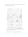
Figure 2: Temperature dependence of the IR absorption spectra of H2O adsorbed
on an Au (111) surface at 98 K.-----------------------------------------------------------------------------12
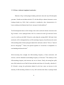
Figure 3: Infrared spectra of thin films of amorphous ice in the OD stretching mode region.----16
Figure 4: Infrared absorbance spectra of unannealed (10 K) binary mixtures of H2O (mole
fraction 33 %) and other components (66 %).-------------------------------------------------------------20
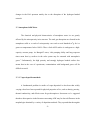
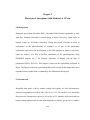
Figure 5: Amount of N2 adsorbed by ASW films versus film thickness.----------------------------26
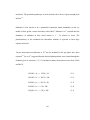
Figure 6: Amount of N2 adsorbed versus growth temperature for 50-bilayer ASW films.--------28
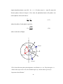
Figure 7: Structure of a cosmic dust particle.------------------------------------------------------------33
Figure 8: Nested Newton spheres photofragments A and B where mA > mB.-----------------------46
Figure 9: Schematic representation of the instrument set up in velocity map imaging------------48
Figure 10: Comparison between images of O+ ions from the photolysis of molecular oxygen at
225 nm----------------------------------------------------------------------------------------------------------48
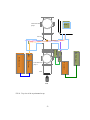
Figure 11: Top view of the experimental set up----------------------------------------------------------53
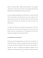
Figure 12: 3D TOF simulated by SIMION 7.0 with repeller, extractor, ground electrodes and
detector---------------------------------------------------------------------------------------------------------56
Figure 13: The xy plane view of the simulated TOF.----------------------------------------------------57
Figure 14: The trajectories originate at y=0 mm with one ion ejected with a 90° elevation angle
and other at 0 ° elevation angle.-----------------------------------------------------------------------------58
Figure 15: Schematic for the projection of ionized photoproducts (originating at point O) on to
the detector ----------------------------------------------------------------------------------------------------60
x
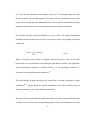
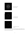
Figure 16: Typical image simulated by the Visual Basic program (top) using broadened velocity
distributions, the Inverted image from the Onion Peeling Program (middle), and the Inverted
image from the Abel Transform (bottom).----------------------------------------------------------------67
Figure 17: Implementation of a “for loop” in LabVIEW- Block Diagram and Front Panel-------74
Figure 18: Communicating with an instrument----------------------------------------------------------75
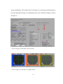
Figure 19: Schematic for the data acquisition system using VIs---------------------------------------78
Figure 20: Communication with the device---------------------------------------------------------------79
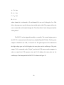
Figure 21: Front panel of power supply-------------------------------------------------------------------80
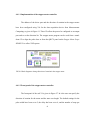
Figure 22: DG 535 front panel------------------------------------------------------------------------------83
Figure 23: DAQ in the PCI 6602E VI---------------------------------------------------------------------86
Figure 24: Front Panel of PCI 6602 VI--------------------------------------------------------------------88
Figure 25: Stepper motor controller and data acquisition device--------------------------------------90
Figure 26: Block diagram to change direction of rotation in the stepper motor---------------------91
Figure 27: Front Panel of the Stepper Motor sub VI-----------------------------------------------------92
Figure 28: Front panel of the Stepper Motor Scope REMPI VI----------------------------------------93
Figure 29: Imaging VI, front panel 1 for user inputs-----------------------------------------------------97
Figure 30: Imaging VI, front panel 2 to display images-------------------------------------------------97
Figure 31: Imaging VI, block diagram---------------------------------------------------------------------98
Figure 32: Evolution of features in CH3OH irradiation. MF= methyl formate.--------------------103
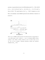
Figure 33: Schematic illustration of the experiment.---------------------------------------------------106
Figure 34: Detection of the photofragment from the surface.-----------------------------------------109
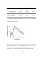
Figure 35: (a) (2+1) REMPI excitation spectrum of CH3 radicals from the 157 nm photolysis of a
fresh ASM sample at 90 K, recorded at t = 6.0 μs .
(b) Simulated REMPI excitation spectrum of CH3 radicals--------------------------------------------111
xi
Figure 36: TOF spectrum of CH3 radicals from the 157 nm photolysis of a fresh ASM sample,
monitoring on the Q branch of the (2+1) REMPI spectrum shown in Fig. 35.----------------------112
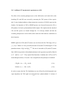
Figure 37: (a) (2+1) REMPI excitation spectrum of OH radicals from the 157 nm photolysis of a
fresh ASM sample at 90 K, recorded at t = 2.0 μs .
(b) Simulation of the D 2 Σ − (v ' = 0 ) ← X 2 Π (v " = 0) two–photon excitation spectrum of OH
assuming a Boltzmann rotational state population distribution with Trot = 300 K. ---------------114
Figure 38: TOF spectra of OH radicals from the 157 nm photolysis of a fresh ASM sample,
obtained by monitoring
(a) the R1(1)+R1(5) line in the OH D 2 Σ − (v ' = 0 ) ← X 2 Π (v " = 0) two–photon transition and
(b) the R1(2) line in the OH 32 Σ − (v ' = 0 ) ← X 2 Π (v " = 1) two–photon transition.-------------------115
Figure 39: (a) (2+1) REMPI excitation spectrum of OH radicals from the 157 nm photolysis of a
fresh ASM sample at 90 K recorded at t = 2.0 μs .
(b) Simulation of relevant parts of the overlapping D 2 Σ − (v ' = 1) ← X 2 Π (v " = 0) and
32 Σ − (v ' = 0 ) ← X 2 Π (v " = 1) two–photon transitions of OH--------------------------------------------116
xii
List of Tables
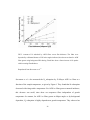
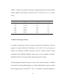
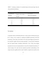
Table 1: Results for the radius of the image and magnification factor based different voltages
applied to the electrodes to ions with 15 amu mass and 1 eV of kinetic energy-------------------------------------------------------------------------------------------------------------------------------------59
Table 2: Anisotropy parameters for simulated image and inverted image from the velocity
broadened distribution----------------------------------------------------------------------------------------68
Table 3: Translational and rotational temperatures and energies of CH3 (v = 0) products.------------------------------------------------------------------------------------------------------------------------112
Table 4: Translational and rotational temperatures and energies of OH (v = 0 and 1) products.---------------------------------------------------------------------------------------------------------------------114
xiii
Chapter 1
Introduction
The investigation of the physical and chemical properties of vapor-deposited ice
has received much attention in the recent years, primarily due to important
astrochemical1-3 and atmospheric4-6 implications. Water ice in the cold, dense regions of
interstellar clouds is a medium for photochemical reactions when exposed to ultraviolet
(UV) radiation.7, 8 On earth, polar regions act as sinks for atmospheric pollutants and UV
photolysis of these compounds produces photoproducts that impact the environment. For
example, heterogeneous reactions between water ice and molecules such as HCl,
ClONO2, and N2O5 in the stratosphere play a central role in the occurrence of the
Antarctic ozone hole.4 Furthermore, simple molecules such as CH3OH, NH3, CO, H2
found on interstellar ices are considered to be the building blocks of the solar system as
their interaction with UV radiation gives rise to complex molecules in molecular
clouds.9,10 Therefore, studies of ice photochemistry in the interstellar medium, in the
polar regions and in the laboratory are of great importance.
With the novel Velocity Map Imaging apparatus under development at Queen’s
University, photochemical reactions on amorphous or polycrystalline ice and their
contaminants can be studied in a controlled lab environment. The photoproducts, which
are formed after irradiation of the ice matrix with a UV laser pulse, are detected quantum
state selectively using a second UV laser through the resonance-enhanced multiphoton
1
ionization (REMPI) technique. The nascent photoproducts are then detected by projection
on a position sensitive detector and their velocity and angular distributions are recorded.
This process is called velocity map imaging (VMI). Using energy and momentum
conservation it is then possible to calculate the energy transferred to the ice matrix. By
characterizing the structural changes that take place in the ice matrix through Fourier
Transform Infrared (FT-IR) spectroscopy, it is possible to obtain even more detail on the
reaction mechanisms between water ice molecules and the photoproducts. The
determination of kinetic and internal energy distributions of the nascent desorbed species
together with the spectroscopic signatures of the ice matrix and the stable trapped
photoproducts is expected to provide the complete photochemical mechanism.
Preliminary work in support of the development of this apparatus has been conducted
through a collaborative study involving the author and the Kawasaki Group at Kyoto
University using a similar machine, albeit without velocity map imaging capabilities. The
experiments with the Kawasaki group illustrate the capabilities and limits of the state
selective detection of photoproducts following methanol ice photolysis.
In chapter 2 of this thesis an overview of the vast literature on the photochemistry of
amorphous solid water and polycrystalline ice with a special emphasis on experimental
studies of photoinduced reactions is provided. The phases of water ice found in
interstellar ices, the properties of vapor-deposited water ice, spectroscopic characteristics
of the ice matrix, the correlation between growth conditions and structure, and effects of
photolysis on the ice matrix are presented.
2
The VMI apparatus at Queen’s University and in particular the ion optics and software
components are presented in Chapter 3. The kinetic and angular distributions of desorbed
photoproducts can be determined by the back projection of the raw image of
photofragments. A back projection method based on a Monte-Carlo simulation is
presented in this section. The ability to synchronize the operation of individual
instruments in the VMI apparatus will be critical in conducting an automated experiment.
In Chapter 4, the programming of the instrumental components using LabVIEW 8.6 is
discussed. Experimental components which were modified or constructed during the
course of this work are also briefly described.
The mechanisms and dynamics of the production of CH3 and OH from the 157 nm
photodissociation of amorphous solid methanol at 90 K serves as a guide as to the data
that may be expected. Preliminary studies on the photolysis of methanol ice were
conducted using a TOF-MS apparatus at Kyoto University. In the final chapter the stateselective detection of OH and CH3 photoproducts from the 157 nm photolysis of methanol
ice is discussed and their REMPI spectra analysed. A plausible reaction mechanism and
the energetics of the reaction are presented.
3
References for Chapter 1
1
G. B. Hansen, T. B. MsCord, J. Geophys. Res., 109, E01012 (2004).
2
B. A. Smith, L. Soderbolem, R. Beebe, J. Joyce, G. Briggs, A. Bunker, S. A. Collins, C.
J. Hansen, T.V. Johnson, J. L. Mitchell, R. J. Terrile, M. Carr, A. F. Cook II, J. Cuzzi, J.
B. Pollack, G. E. Danielson, A. Ingersoll, M. E. Davies, G. E. Hunt, H. Masursky, E.
Shoemaker, D. Morrison, T. Owen, C. Sagan, J. Ververka, R. Strom and V. E. Suomi,
Science, 212, 163 (1981).
3
F. L. Whipple, Astrophys. J., 11, 375 (1950).
4
M. A. Tolbert, A. M. Middlebrook, J. Geophys. Res., 95, 22423 (1990).
5
T. G. Koch, S. F. Banham, J. R. Sodeau, A. B. Horn, M. R. S. McCoustra, and M. A.
Chesters, J. Geophys. Res., 102, 1513 (1997).
6
A. B. Horn, T. Koch, M. A. Chesters, M. R. S. McCoustra, and J. R. Sodeau, J. Phys.
Chem. 98, 946 (1991).
7
S. Andersson, A. Al-Halabi, G.-J. Kroes, and E. W. Dishoeck, J. Chem. Phys. 124,
064715 (2006).
8
L. J. Allamandola, M. P. Bernstein, S. A. Sanford, and R. L. Walker, Space Sci. Rev. 90,
219 (1999).
9
N. Watanabe, and A. Kouchi, Prog. Surf. Sci. 83, 439 (2008).
10
E.Herbst, Chem. Soc. Rev. 30, 168 (2001).
4
Chapter 2
Literature Review
2.0 Introduction
Amorphous Solid Water (ASW) is a major constituent in interstellar clouds1,
comets2, satellites of outer planets3, and icy grain mantles4. Thus, it has important
astronomical implications. Also, water ice in the cubic or amorphous phase has been
reported as a major component of the surface of many satellites and planetary rings.3 On
earth, heterogeneous reactions, occurring on the surfaces of polar stratospheric cloud
particles, are recognized to play a central role in the photochemical mechanism
responsible for the occurrence of the Antarctic ozone hole.1 The crystallization process of
ASW is important in physical phenomena associated with ices such as sublimation, the
outgassing of volatile molecules, and changes in the thermal conductivity.2,3 These
properties are controlled to a large extent by changes in the hydrogen bonded network of
the water during heating.2 By characterizing the structural changes that occur within water
ice, it may be possible to understand the chemistry of cometary and interstellar ice and
stratospheric ice particles. Hence, the study of water ice at low temperatures and the
ability of water ice to trap gases have received much attention. Photochemistry of water
ice plays an important role in interstellar grain chemistry. For this reason, primary and
secondary photodissociation reactions taking place on water have received extensive
attention because of their importance in atmospheric chemistry and astrophysics.1-6 This
5
chapter concerns the chemical behavior and structure of the ice surface, in particular with
regards to the spectroscopy and the photolysis of surface ice films. This will be followed
by a discussion of the photochemistry of water ice and of constituents in ice.
2. 1 Structure and Formation of water ice
The equilibrium structure within which a material crystallizes under given
conditions of temperature and pressure is determined by the interaction forces between its
molecules. The properties of ice have been interpreted by their crystal structure, forces
between their constituent molecules, and their energy levels. The crystal structure of ice is
formed with water molecules linked to each other so that each proton of one molecule is
directed towards a lone pair electron hybrid of a neighboring molecule. The oxygen atoms
in ice are arranged so that they are at the centre of a tetrahedron, with each oxygen atom
positioned 2.76 Å away from four other oxygen atoms.3-5
The structure of water-rich ice in astrophysical environments is usually not that of the
familiar thermodynamically stable hexagonal crystalline polymorph (Ih) found almost
exclusively on Earth. Rather, astrophysical water ice is often observed to be in an
amorphous form.2 Temperature is the main factor determining the crystallographic phase
of ice grown from the gas phase at low pressures.3,4
6
Narten et al.5 reported that there are two evidently distinctive forms of amorphous ice
which differ in density as well as in the second nearest-neighbour oxygen-oxygen
distribution. The low-density form was estimated to be 0.94 g/cm3 at 77 K and the highdensity (Iah) 1.1 g/cm3 at 10 K. The nearest-neighbour O-O separation was 2.76 Å in the
low-density form. The high-density form had similar an X-ray diffraction pattern similar
to low-density amorphous ice. However, it showed an additional peak at 3.3 Å. Narten et
al.5 suggested that the increase in density was a consequence of water molecules
occupying the distance between the first and second nearest neighbour at the interstitial
sites of the network. The additional peak was caused by such water molecules and was the
first indication of the occurrence of structural polymorphs of water.6 Low-density
amorphous ice produced by water vapour deposition below 130 K was determined to be a
highly porous open network with a surface area of 150 - 500 m2/g. This form of ice also
has a noteworthy concentration of surface OH groups as observed through the
measurements of surface area, density of ice films and IR spectroscopy of water ice.5-8
Furthermore, Jenniskens and Blake8 designed experiments to simulate interstellar ices by
observing the structural changes of vapor-deposited on water ice in vacuum between
temperatures of 15 to 188 K. They reported the existence of three amorphous forms and
two crystalline forms of water ice. High-density amorphous water ice (Iah) is found at 15
K, the low-density form (Ial) between 38 to 68 K, and the restrained amorphous form (Iar)
preceding cubic ice (Ic) at 131 K.2 When amorphous ice films are further annealed,
crystalline ice transfers to polycrystalline cubic ice (Ic) and hexagonal ice (Ih). The Ih
7
phase prevalent on earth can also be produced directly by condensation onto a substrate
cooled to temperatures above 190 K.3 Condensation below 190 K but above 135 K leads
to Ic.3 If warmed between 160 - 200 K Ic will transform irreversibly into Ih. This wide
temperature range has been attributed to the dependence of the crystallization temperature
on the size of cubic ice crystals. These observations imply that the crystallization process,
which commences just above the glass-to-liquid transition temperature, is incomplete
because fragments of the non-crystalline microphases co-exists with Ic up to 200 K.8,9
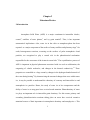
Amorphous ice is the dominant form at temperatures below 130 K. This phase of ice
converts to Ic at a rate that depends on the temperature as given in Figure 1. Iar coexists
with Ic from 148 K until 188 K. The existence of Iar is responsible for the irregular gas
retention and gas release from water rich ices at temperatures above 150 K.8 Figure 1
illustrates the existence of amorphous and crystalline ices at different temperatures.
8
Hexagonal
RestrainedCubic
Ice
Cubic Ice
Ih
Polycrystalline
Cubic Ice
I c
135-190 K
Above 190 K
Restrained
Amorphous Ice
I ar h
131 K Low Density
Amorphous Ice
I al 38 -68 K
High Density
Amorphous Ice
I ah
15 K FIG.1. Structural dependence of ice on temperature.
9
In addition to this, Berland et al.10 reported that the density of vapor-deposited ice films as
a function of substrate temperature. At 35 K, the density of ice films was found to be 0.68
g/cm3. This is considerably lower than 0.93 g/cm3 for ice Ic. This low density is due to the
formation of microporous amorphous ice. Furthermore, the density increased rapidly from
0.68 – 0.78 g/cm3 for temperatures between 30 – 60 K, and from 0.80 – 0.93 g/cm3 for
temperatures between 80 K – 120 K. A density of 0.93 g/cm3 was reported for ice films
between temperatures 120 K - 150 K.
The structure of unannealed amorphous ice is found to have greater dispersion of O…O…O
angles and nearest neighbor O-O separations and a larger mean separation than that of
annealed amorphous and polycrystalline ice.9 This gives rise to a more disordered
structure in unannealed amorphous ice and results in a wider distribution of weaker
hydrogen bond strengths. Of the solid forms of H2O the unannealed amorphous ice is the
most comparable structure to that of liquid water. The transition from Iah to Ial is
accountable for the diffusion and recombination of radicals of interstellar ices processed
by ultraviolet radiation at low temperatures.8
10
2. 2 Spectroscopic studies of vapor-deposited ice films
2. 2. 1 Pure H2O
The infrared spectra of all forms of solid water are characterized by four
absorption bands. A sharp band is observed for the dangling OH-stretching mode from the
ice surface at 3700 cm-1. This intense band corresponds to the symmetric (υ1) and
antisymmetric (υ3) modes in the isolated water molecule. A broad band is observed at
3370 cm-1 due to the OH-stretching mode in the bulk of amorphous ice at 98 K. The third
band (1665 cm-1, υ2) is a result of the bending mode. The fourth prominent band observed
at 763 cm-1 is a consequence of libration, i.e. the hindered rotation of the water molecule.
In addition, comparatively weak combination bands are observed at 2205 cm-1 (3 υL or
υ2+ υL).9-12 The IR absorption spectra of H2O adsorbed on Au (111) are given in Figure 2.
The IR absorption features observed in the water molecule are dependent on the hydrogen
bonding of the system. The difference between the vibration frequencies of H2O
molecules in the gas phase and the frequency in unannealed amorphous ice for the
bending mode is +70 cm-1 and for the OH-stretching mode -450 cm-1.9 Elevated
frequencies in libration and bending modes may be observed due to the presence of a
strong hydrogen bonded network. Strong hydrogen bonds hinder libration and bending
and weaken the normal OH-stretching frequencies.
11
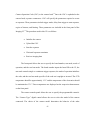
FIG.2. Temperature dependence of the IR absorption spectra of H2O adsorbed on an Au (111)
surface at 98 K. H2O was first adsorbed at 98 K, and then the substrate was heated step wisely to
the indicated temperature.
Reproduced from Sato et al.12
12
The effects of hydrogen bonding on the frequency and width of IR absorption features in
amorphous ice was investigated by Hagen et al.11 They reported that when amorphous ice
is deposited at 10 K, and warmed up to 130 K, the bulk OH-stretching band shifted to
3250 cm-1, the line width narrowed, the peak intensity increased and the libration
frequency increased.9 This was due to the increased strength in the hydrogen bond. Upon
annealing to 130 K, amorphous ice deposited at 10 K undergoes an irreversible
transformation to a more ordered form. With the annealing process, the distance between
neighboring O-O positions decreases and the molecule reorients to optimize the
preferably linear O-H…O bond angles. The smaller O-O separations result in strengthened
hydrogen bonds. Jenniskens and Blake8 reported that irreversible changes continue to
occur in the same parameters when amorphous ice is kept at 140 K for a prolonged time.8
These changes correspond to the transformation from amorphous ice to crystalline ice (Ic).
Since these spectral changes start at temperatures as low as 120 K, it has been inferred
that the phase change from amorphous ice to crystalline occurs above 120 K. The
transformation is completed within 45 min.
13
2. 2. 2 Dangling OH
A fundamental characteristic of low-density amorphous ice is its microporosity.
Amorphous ice formed below 90 K is a microporous network with a large surface area of
approximately 400 m2/g due to the presence of nanoscale pores.
13
Pore widths were
measured to be less than 2 nm.13
The conventional four tetrahedral hydrogen bonds in water molecules are indicative of the
condensed phase of H2O. However, Rowland et al.13 observed that water molecules on the
pore surface cannot form these 4- coordinated/ tetrahedral hydrogen bonds. They reported
that, as a consequence, dangling O-H groups that are weakly hydrogen bonded are formed
on the pore surface. Vibrational spectroscopic studies of vapor-deposited ice films by
Buch and Devlin14 showed evidence of dangling O-H bonds for ice films deposited at low
temperatures. The existence of these dangling O-H bonds designates vacancies in the ice
network that are a distinctive feature of microporous ice films.
The vacancies denote the tendency to form hydrogen bonds with incident molecules, as a
consequence of the highly polarized surface. Consequently, an incident molecule with a
hydrogen bond receptor or donor group such as HCl will have a higher probability of
sticking to the surface and leading to hydrogen bond formation.
14
Two kinds of dangling bonds are signified by a doublet at 3720 and 3696 cm-1 in lowdensity amorphous ice deposited below 15 K, and at 2748 and 2727 cm-1 for D2O as
shown in Figure 3.13,14
(a) Dangling O-H belonging to 3-coordinated molecules, with two hydrogen
bonds via O and one via H, which gives rise to the low frequency form
(b) Dangling O-H belonging to 2-coordinated molecules, with one hydrogen bond
via O and one via H which gives rise to the high frequency form.14
The higher and lower frequency features of each doublet have been assigned to 2coordinated and 3-coordinated water molecules respectively.14
15
FIG.3. Infrared spectra of thin films of amorphous ice in the OD stretching mode
region:
(a) Pure D2O at 15 K
(b) unexchanged 50% D2O / 50% H2O at 15 K
(c and d) sample of part b annealed 10 min at 60 and 120 K
Adapted from Rowland et al.13
16
Buch and Devlin14 reported that, upon annealing the amorphous ice film to 60 K, the 2coordinate high-frequency component of the doublet was entirely diminished. However,
the low-frequency component continued to remain in place. When amorphous ice is
further annealed to 120 K, all evidence of the dangling OH disappears entirely. This
disappearance is a consequence of the surface restructuring that take place alongside the
annealing process, which leads to a reduction in the amount of internal surface in the solid
ice. Similar results are exhibited by the spectra for the OD-stretching mode, and its IR
absorption features are presented in Figure 3 as a function of both temperature and
fraction of D2O.
2. 2. 2. 1 Temperature and pressure dependence of the dangling OH bond
The temperature and pressure dependence of the IR absorption features are
imperative to understand the formation of microporous ice at low temperatures and the
collapse of micropores during annealing at 120 K.13 The collapse of the micropores
accompanies the densification and a change in the structural organization of the water ice
network.10 The temperature dependence of the dangling OH bond signifies that there are
two regions for structural transitions in vapor-deposited ice that corresponds
approximately to the regions where the density changes rapidly. Hence, the spectral
feature of the dangling OH bond can also be used as a means to investigate the surface
properties of water ice.
17
In the ballistic deposition model of ice, the incident H2O molecules are deposited on the
ice surface with a sticking probability of one, as they encounter unoccupied sites.15 H2O
desorption is negligible at temperatures below 140 K.10 Hence, an incident H2O molecule
brought to the water ice surface will be either buried by a successive inward-bound H2O
molecule or may diffuse to an unoccupied site in the ice multilayer. The time available for
the admolecules to diffuse before they are buried by the H2O layer is dependent on the
incident H2O flux.10 At a high vapour deposition pressure, molecules are buried faster
than they can diffuse. As the temperature decreases at a fixed deposition rate, it is less
likely that a given molecule will have sufficient energy to the find a more favourable site
in the network. If the molecule is buried in a higher orientation, more micropores and
dangling bonds result within the ice bulk.15
2. 2. 3 Interaction with other species
Tielens et al. 9 conducted an extensive study on the interaction of amorphous ice
with other species. The spectroscopic properties of water ice undergo changes upon
interaction with impinging molecular species. Adsorbent species may alter the structure of
amorphous solid water, based on factors such as their size, shape, and hydrogen bonding
ability. Due to the existence of impurities, the degree of intermolecular coupling becomes
smaller, and the hydrogen bonds become weaker because of increased O-O separation.9,16
This phenomenon leads to an increase in the OH-stretching frequency and a decrease in
librational and bending frequencies. In addition to these changes, the OH-stretching band
18
was reported to have become less intense as a result of the reduction in induced
polarization. 9,16
2. 2. 4 Species with incomplete hydrogen bonding
Molecules that are incident on the ice surface and that show deficiencies in
forming hydrogen bonds can be identified by distinguishing features observed in the IR
absorption spectra. 9,17 The following features can be seen as a result of the incomplete
hydrogen bonding in the H2O network as given in Figure 4:
(a) The terminal OH group in the water molecule can be identified by a distinct OHstretching frequency around 3700 cm-1 in the presence of dilutant molecules that are
incapable of accommodating hydrogen atoms to form hydrogen bonds (e.g., CH4, Ar, O2
or CO).
(b) The main OH-stretching band yields a shoulder at 3220 cm-1 when water molecules do
not accept any H atoms at the O atom lone pair, but are able to donate H atoms to form
hydrogen bonds (e.g., C6H6, C2H2).
Since H2O molecules which do not accommodate hydrogen atoms are able to position
themselves in a complementary placement to form hydrogen bonds, the 3220 cm-1 peak is
observed at a lower frequency than that of the main OH stretching band.9,16 The structural
disparities of the dilutant species in terms of shape and size will result in dissimilarities in
19
their interaction with pure amorphous ice. These differences have been determined to
increase in the order of CH4, Ar, O2 and CO.9
FIG.4. Infrared absorbance spectra of unannealed (10 K) binary mixtures of H2O (mole
fraction 33 %) and other components (66 %).
Adapted from Tielens et al.9 . Line intensity has been increased for clarity.
20
2. 2. 5 Bases, Acids and Amphoteric molecules
Dilution of H2O with hydrogen bonding molecules alters the H2O IR absorption
spectrum. Consider an incident molecule ‘B’ with the ability to donate electrons to create
hydrogen bonds (e.g. NH3). Such a molecule is considered to have characteristics of a
base according to the Bronsted and Lewis concepts of acids and bases.9
The IR absorption features in H2O change when such a molecule donates electrons to the
H2O network. A new hydrogen bond, O-H…B, is observed in the H2O network.9 In the
case of a weak base, the HOH…B bond is weaker than the existing HOH…OH2 bond. Such
molecules will be distinguished by an OH-stretching frequency found between the main
OH-stretching band of fully hydrogen bonded H2O molecules and the 3700 cm-1 band of
the free OH groups.9,17 Hence, the spectral signature of a weak base is comparable to a
non-bonding incident molecule.9
With increasing base strength, the OH-stretching frequency of these molecules will
decrease, and the librational and bending frequency will increase.9 The intensity of the
OH-stretching frequency also increases due to two factors. Firstly, the strong base pulls
more H2O molecules out of the H2O network than weak bases do. Secondly, when the OH…B bond is strong, the polarization induced by the base causes an increase in the
intensity of OH-stretching vibration in every H2O molecule that forms a hydrogen bond
21
with the base.9 The spectra of mixtures of H2O and strong bases such as CH3NH2 and
NH3 reflect this behavior. 9
Consider an incident molecule HA with the ability to donate hydrogen atoms and accept
electrons to create hydrogen bonds. Such a molecule is considered to have characteristics
of an acid according to the Bronsted and Lewis concepts of acids and bases (e.g. HCl).
‘A’ is a conjugate base of the acid HA and will form a hydrogen bond O…H-A. In this
case, the hydrogen atom accepting the H2O molecule acts as the base.9 The conjugate base
‘A’ competes with H2O for the hydrogen atom.
If the H2O…HA bond is stronger than the HOH…OH2 bond, the weakening of the bonds
in the H2O network causes the OH-stretching mode to shift to a lower frequency, while
the frequencies of libration and bending increase.9,16 In the case of weak acids, this
process will lead to incompletely hydrogen bonded H2O molecules in the H2O network.
This incomplete bonding will cause the 3220 cm-1 shoulder to increase. Tielens et al.
observed that the 3220 cm-1 shoulder will disappear if the strength of the hydrogen bonds
between H2O and the acid is equal to that between two H2O molecules.9
An incident molecule with the capacity to donate hydrogen atoms, as well as accept
hydrogen atoms to form hydrogen bonds, is characterized as an amphoteric. The effect of
an amphoteric on the H2O spectrum will be a grouping of the characteristics explained
above.9 For example, methanol has amphoteric character like water and causes small
22
changes in the H2O spectrum mainly due to the disruption of the hydrogen bonded
network.
2. 3 Amorphous Solid Water
The chemical and physical characteristics of amorphous water ice are greatly
affected by the microporosity in its structure. The total gas absorption area formed in the
amorphous solid as a result of microporosity can reach several hundred m2/g for ice
grown at temperatures below 100 K.3 Thus a fresh ASW surface is analogous to a highcapacity vacuum pump. As Baragiola3 notes, “this pumping ability and long exposure
times mean that icy surfaces in the solar system may be saturated with atmospheric
gases.” Unfortunately, the high porosity and strongly hydrogen bonded surface also
means that in the case of experiments, contamination with background gases will be
difficult to avoid.
2. 3. 1 Vapor deposition methods
A fundamental problem in studies of vapor-deposited ice has been that widely
varying values have been reported for physical properties of ice, such as density, porosity,
thermal conductivity, and effective area for gas absorption.20 Stevenson et al.15 suggested
that these discrepancies in the literature concerning ASW may be due to differences in the
morphologies obtained by a variety of deposition methods. They reported that the angular
23
distribution of incident H2O flux used to grow the ASW films in a vacuum is a critical
factor influencing the ASW morphology at low temperatures. They demonstrated that, by
systematically varying the incident angle of the H2O flux during deposition, the controlled
growth of nonporous to highly porous ASW could be achieved.15
In astrophysical environments, the morphology of ASW will depend on the two possible
mechanisms of formation: (a) direct deposition and (b) omni-directional deposition.
Direct deposition may occur in the rings of Saturn, where it has been reported that water
molecules sputtered from the outer rings accumulate on the inner rings; it may also occur
when a body such as a dust grain is passing through a molecular cloud with a large
relative velocity.21 Porous ASW may form by means of omni-directional deposition of
water molecules and may occur during the formation of comets.21 In the light of these
occurrences, the morphology of thin ASW films has been investigated by two different
methods: 18
(a) Using highly collimated effusive H2O beams (i.e., “direct deposition”)
(b) Introducing water vapor through a leak valve (i.e., “background deposition”)
Kimmel et al.18 observed that beam-deposited ASW films had an area of uniform
thickness surrounded by an area of decreasing thickness, contained within the diameter of
the sample. The films grown by ambient vapor were uniform across the sample.
24
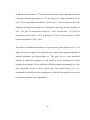
Stevenson et al.15 compared the N2 adsorption of ice films varying in thickness, grown
using both of these methods between 22 -145 K by dosing at different incident angles. For
large incidence angles, the N2 adsorption increased almost linearly with thickness, as
given by Figure 4. The N2 adsorption of ASW films grown by the background deposition
method was higher than the adsorption of ASW films grown by collimated H2O beams at
high angles of incidence. The linear increase of the N2 adsorption is indicative of the
highly inter-connected pore structure that allows N2 to penetrate the ASW film. Stevenson
et al.15 reported that the N2 adsorption on ASW ice films grown at normal incidence was
much smaller and almost independent of thickness. Moreover, they found that the ASW
behaved as a denser film without a network of pores and that adsorption mainly took
place through the external surface. The results were in agreement with the ballistic
deposition model, which considers the effects of coarseness in the surface caused by
random vapor deposition.
25
FIG.5. Amount of N2 adsorbed by ASW films versus film thickness. The films were
deposited by collimated beams at 22 K at the angles indicated; also shown are data for ASW
films grown using background H2O dosing. Fitted lines show a linear increase in N2 uptake
with increasing film thickness.
Reproduced from Stevenson et al.15
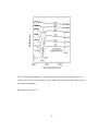
Stevenson et al.15 also measured the N2 adsorption by 50 bilayer ASW ice films as a
function of the sample temperature, as given by Figure 6. They found that N2 adsorption
decreased with rising surface temperature. For ASW ice films grown at normal incidence,
this decrease was small, since these are nonporous films independent of growth
temperature. In contrast, for ASW ice films grown at oblique angles or by background
deposition, N2 adsorption is highly dependent on growth temperature. They observed an
26
extraordinarily large surface area of 2700 m2/g at 22 K and 640 m2/g at 77 K for ASW
films grown from background deposition and reported a linear increase of porosity with
time. With these observations, they proposed that large surface areas observed at low
temperatures and oblique angles of the incident were a result of the connection of the
internal surface being connected to the external surface of the film through a network of
pores.
The porous character of low-density amorphous ice is caused by thermo-kinetic
deposition. The incoming water molecules that adsorb at the surface may lose most of
their energy well before finding the most stable site.9
27
FIG.6. Amount of N2 adsorbed versus growth temperature for 50-bilayer ASW films. The
films were deposited by collimated beams at the angles indicated; also shown are data for
ASW films grown using background H2O dosing. The dotted lines through the data are to
guide the eye. For the thin films and low deposition rates used in these experiments, the
ASW film temperature and the Pt(111) temperature are essentially identical ( Δ T<< 0.1 K).
Reproduced from Stevenson et al.15
28
2. 3. 2 Micropores
Vapor-deposited ice at 12 K grows with an extremely uneven surface that results
in a microporous network with 5-10% of the molecules on the ice surface.22 When water
molecules incident on the ice surface have inadequate time to move to a suitable site
before being covered by subsequent adlayers, they are buried in random orientations and
leave gaps within the bulk ice. As a result, microporous networks are formed in the ice
film. When these gaps are of a sufficient width, they prevent the formation of hydrogen
bonds across the pore. Hence, 3-coordinate OH groups that are non hydrogen bonding are
formed at the pore surface.23 Devlin and Buch22 observed the loss of surface OH
vibrational signature between temperatures of 30 - 60 K.
They proposed that the
weakening of the IR absorption signal for dangling OH groups was a consequence of the
solid water structure becoming less dense as the water molecules achieve a fuller coordination. This process yields an open tetrahedral network.22
Zondlo et al.23 investigated the behavior of dangling OH bonds in vapor-deposited ice
between 90 and 120 K and reported that the intensity of the dangling OH feature
increased linearly with the thickness of the ice film. They proposed that the majority of
the dangling OH was formed on the micropores of ice inside the condensed ice bulk. In
addition, they suggested that low substrate temperatures and fast deposition rates led to
the profusion of micropores in the condensed ice network.
29
Microporosity is related to the retention of gas in amorphous ice. Studies of gas
adsorption on vapor-deposited amorphous ice have revealed that the amount of gas uptake
is consistent with microporosity and large surface areas of up to hundreds of m2/g.
However, parameters such as pore shape, structure, and adsorption energies remain
unknown.24, 25
In a study on the characteristics of pores using gas adsorption isotherms, Raut et al.24
reported the existence of dual pore structure in the form of mesopores and micropores.
They observed that the CH4 adsorption isotherms for ice films formed by background
deposition of water vapor were different from those for collimated beams. Films formed
by background deposition demonstrated a step in the isotherms and less adsorption at low
pressures. This observation led them to propose that the micropores formed by these two
methods were dissimilar. In addition, they reported that films deposited at 77° incidence
to the surface from a collimated beam developed both micro and mesopores. Upon
annealing to 140 K, where the ice crystallizes, the micropores were destroyed while the
mesopores were sustained.
2. 3. 3 Trapping of gas
The studies on the ability of water ice to trap and release gas have important
implications linked to the outgassing process of comets.24-27 These studies help
characterize the pores connected to the outside of the ice but not the enclosed pores.3
30
Gases can be trapped by condensation on the ice surface at low temperatures below gas
freezing temperature, or by the formation of clathrate hydrates in which the gas molecules
are trapped in cages formed in the water ice only in the presence of the gas.26,27 The high
porosity of the amorphous ice allows large volumes of gas to settle in the vast number of
cracks and holes. When the volume is filled and a monolayer of adsorbed gas is formed,
the surplus gas freezes on the ice surface.26
Bar-Nun et al.27 reported that CO, CH4, N2 and Ar gases trapped in are released at four
temperature ranges:
(a) 30- 60 K: some of the holes are reopened and the gas frozen on water ice evaporates,
while from 80- 120 K the annealing locks gas inside a compact and impermeable matrix.
(b) 135- 155 K: the trapped gas is squeezed out during the transformation from
amorphous into less porous cubic ice.
(c) 160- 175 K: deeply buried gas is released during the transformation of cubic ice into
hexagonal ice.
(d) 165- 190 K: gas and water are released simultaneously, during the evaporation of a
clathrate-hydrate.
With increasing growth temperature, the gas absorption ability or porosity decreases
greatly.15ASW formed at temperatures below 90 K is a highly adsorbent solid with a
surface area of approximately 400 m2/g.28 At temperatures above 90 K, Stevenson et al.15
observed that ASW films essentially had the same adsorption as the non porous
31
crystalline ice formed at 145 K. Rowland et al.13 reported that dangling O-H bonds
diminished by warming to temperatures near 60 K. They concluded that micropores that
continue to remain in ice above 60 K have no access to the surface.
In a study on the gas retention of ASW, Baragiola3 reported that ~1.7 nm cavities in ASW
disappear or join together at 100 K, but some cavities continue to remain even after
warming beyond the crystallization temperature.29 Upon annealing ASW becomes a
compact solid with closed pores and this yields a reduction in gas adsorption.3,24 Horimoto
et al.30 investigated methane adsorption using infrared spectroscopy and proposed that gas
adsorption was rendered by cavities larger than micropores which collapse upon
annealing to 60 K. They concluded that micropores are not affected until 80 K and
collapse only at 120 K.
2. 4 Photolysis of ASW
The effects of ultraviolet radiation on water ice are important in the chemistry of
both atmospheric and interstellar ices. Significant progress has been made in
understanding the chemical and physical processes following the absorption of Ultraviolet
(UV) photons by condensed phases of water.
Cosmic dust is formed from gases of refractory elements such as Mg, Si, O and C around
1000 K.4, 32-34 Dust diffuses to interstellar space and gradually forms a molecular cloud.
32
Herbst33 has reported extensively on the formation of molecular clouds. Watanabe et al.4
reported that a significant amount of radiation penetrates through relatively thin molecular
clouds since their inception. As a result of photoerosion, volatile molecules cannot remain
stable at the surface of the molecular cloud. Hence, dust is found as bare silicate or
carbonaceous particles in the molecular cloud.4 The temperature of the molecular cloud
begins to lessen as the density of the dust particles increases. This process is followed by
a reduction in the photon field due to optical absorption.4
A presolar molecular cloud33 is formed when a molecular cloud is cooled from 1000 K to
10 – 100 K. Due to the exceeding reduction in the photon field, atoms and molecules
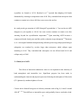
deposit on the dust surfaces and can now form a solid ice mantle.4 At the end of this
process a presolar molecular cloud contains dust consisting of core-mantle particles and
an additional outer mantle of volatile ices dominated by H2O as given in Figure7. 33
Solid ice mantle
Organic
0.5 µm
Silicate
Refractory Material
FIG.7. Structure of a cosmic dust particle. Adapted from Herbst.33
33
Over 120 molecular species of ions and complex organic molecules have been detected in
molecular clouds. These species evolve from atoms and other simple molecules through
surface mediated chemical reactions.4,33,34 Almost 50 percent of the species found in
molecular clouds are familiar terrestrial species such as water, ammonia, formaldehyde,
and simple alcohols such as methanol and ethanol.33 The other 50 percent of the species
include positive ions (e.g. H3+, HCO+, H3O+), radicals (e.g. CnH through n = 8), isomers
of stable compounds (e.g. HNC, HCCNC, HOC+), and unusual three-membered rings
(e.g. C3H, C3H2).33 Of course, molecular hydrogen is found to be the dominant species.3234
The second most abundant species is CO.33 The concentration of molecular hydrogen is
reported to be 104 times higher than that of CO.33
Chemical process on ice mantles can be categorized into two types:
(1) Energetic processes caused by radiation.
(2) Non energetic surface reactions in which abundant atoms such as hydrogen and
oxygen play an important role.4
Photons in the range from UV to Vacuum Ultraviolet (VUV) can induce chemical
reactions on ice mantles. Dust shielding a dense molecular cloud makes it difficult for UV
and VUV photons to penetrate the cloud.4,31 The internal UV flux in a dense cloud is
approximately 103 photons cm-2 s-1.35 Although this flux gives one incident photon per
month on a grain, a significant chemical evolution takes place over the life time of a
molecular cloud, which is 106-107 years. Hence, certain processes induced by UV
absorption are important in evolving molecular clouds. 31
34
Within the characteristic temperature range of 10-100 K in molecular clouds, molecules
are typically synthesised through barrier-less ion-molecule reactions in the gas phase and
therefore these gas phase reactions have been studied over a long period.4,31-34 However,
the insight that the profusion of some molecules such as hydrogen molecules cannot be
explained by pure gas phase formation has drawn considerable attention to the surface
reactions on dust grains which account for the formation of these molecules.4
The cosmic ray ionization of hydrogen molecules produced on grains and desorbed into
the interstellar gas is indicated below.33
H2 + cosmic ray → H2+ + e− + cosmic ray
(1.1)
H2+ ion reacts with molecular hydrogen to produce H3+.33
H2+ + H2 → H3+ + H
(1.2)
The H3+ ion is a comparatively abundant species as it does not react with molecular
hydrogen.33 Hence, the H3+ ion serves as a precursor for gas phase reactions in the
molecular cloud with its ability to react with other species.33 For example, the reactions
with atomic oxygen initiate a chain of reactions leading to the production of the
hydronium ion via reactions (1.3), (1.4), and (1.5).33
H3+ + O → OH+ + H2
(1.3)
OH+ + H2 → H2O + H
(1.4)
H2O + H2 → H3O+ + H
(1.5)
35
Besides gas phase reactions, in the cold region of the molecular clouds where dust grains
are covered with the water ice mantle, H2 production through the photolysis of H2O
molecules in icy mantles is important. Yabushita et al.36,37measured kinetic energy and
the rovibrational population of H2 molecules produced by 157 nm photolysis of water ice
at 100 K using the REMPI method. When water ice is exposed to VUV radiation, the H-O
bond ruptures, and this is reported as a photolytic source of hot hydrogen atoms at the
surface of comets and dust grains in the interstellar medium.38 Yabushita et al.36,37
reported that hydrogen molecules on ASW are produced by two distinct mechanisms:
hydrogen abstraction [HAB, reaction (1.6)] and hydrogen recombination [HR, reaction
(1.7)].
HAB : H + HOH → H2 + OH
HR : H + H
(1.6)
→ H2
(1.7)
Since the optical penetration depth of a water ice film at 157 nm is ~100 nm, Yabushita et
al.36,37 proposed that H atoms produced far beneath the ice surface will collide with
surface OH groups that are exposed through the porous surface of ASW to produce
hydrogen molecules.36,37
Andersson et al.31 reported that, unlike in a molecular cloud, multiple photodissociative
events can take place on the water ice surface within a narrow range of time and space
when exposed to a high flux of UV photons. Photofragments released from different sites
36
can react with one another to produce species such as OH, HO2, O2 and H2O2.31 Some
photofragments are observed to be mobile and may move distances of several angstroms
before becoming trapped in sites and they can partake in additional reactions. However,
the recombination process such as the reaction of H and OH to form H2O limits the
possibility of the photofragments reacting further.31
The presence of OH, HO2, and H2O2 products in UV photolysis of ice deposited on solid
Ar has been observed by Gerakines et al.35 The photochemistry of the water molecule is
initiated by reaction (1.8).
H2O + hυ → H + OH
(1.8)
Subsequent steps lead to the production of H2O2 and HO2 as given in reactions (1.9) and
(1.10). 35
OH + OH → H2O2
(1.9)
OH + H2O2→ H2O + HO2
(1.10)
H2O2 has been observed as a minor component of the water ice on the surfaces of Europa,
a satellite of Jupiter and of Enceladus, one of Saturn’s icy moons.39 The UV photolysis of
nitrate on snow grains produces H2O2, which is reported as a precursor for the production
of OH in polar air through secondary photolysis.40 In a study on the formation of H2O2 at
the ice surface following the photodissociation of ASW at 90 K, Yabushita et al.40
proposed a mechanism for this process via reactions (1.11)-(1.13).
H2O + hυ → H + OH
(1.11)
37
OH + OH → H2O2
(1.12)
H2O2+ hυ (300 - 350 nm) → 2OH
(1.13)
Molecular dynamics calculations performed by Andersson et al.31 to simulate the
photodissociation of water ice at 10 K, showed that OH radicals move at most 5 Å
through bulk ice. However, OH radicals released from photodissociation at the surface
were reported to be highly mobile with the ability to travel 80 Å over the surface.31 Since
there is appreciable mobility at 90 K, the distance between many OH radicals will be
comparable with their bimolecular reaction radius so that OH recombination reactions can
produce H2O2 on the ice surface. 40
In addition to the UV initiated reactions of water ice, the heterogeneous reactions that take
place on water-ice particles have attracted considerable attention as well. The molecular
adsorption on ASW is significant in environmental chemistry.12 For example, the release
of oxygen atoms into the atmosphere from NO3⎯ adsorbed on ice is important in the
formation of ozone and in the cycling of NOx in the Arctic and Antarctic boundary
layer.41-44 Davis et al.41 reported that the summertime boundary layer over the South Pole
has elevated levels of NOx, OH and O3. Nitrate plays an important role in snowpack
photochemistry as the precursor for the formation of these oxidizing species as given in
reactions (1.14-1.16). 45
NO3⎯ + hυ (340 nm) → O(3P) + NO2⎯
(1.14)
NO2⎯ + hυ + H+ → NO + OH / HONO
(1.15)
NO2 + hυ → O(3P) + NO
(1.16)
38
Yabushita et al.45 have detected the formation of the oxygen atom via reaction (1.16) and
have reported that these reactions play a central role on air pollution at the South Pole.
Many CO-bearing molecules, including simple organic molecules such as H2CO and
CH3OH, have been discovered abundantly in the ASW mantle of dust grains.35,46 These
molecules serve as important precursors to form complex organic molecules. They require
the chemical processes through surface reactions to produce the observed abundances.4
Since CO exists abundantly on the dust surface, these molecules are considered to evolve
from it. Chapter 5 of this thesis discusses in the photolysis of methanol ice.
2.5 Conclusion
Chemical reactions on the surface of cosmic ice dust play an important role in chemical
evolution. Among the many kinds of molecules observed, the abundances of some major
species such as hydrogen molecules cannot be explained by gas-phase synthesis.
Therefore, surface reactions on cosmic dust are considered for the synthesis of such
molecules. Further research on the reactions that takes place on the water ice surface is
desirable in order to understand the formation and evolution of icy grains in molecular
clouds.
39
References for Chapter 2
1
M. A. Tolbert, A. M. Middlebrook, J. Geophys. Res., 95, 22423 (1990).
2
P. Jenniskens and D. F. Blake, Astrophys. J. 473, 1104 (1996).
3
R.A. Baragiola, Planet. Space Sci. 51, 953 (2003).
4
N. Watanabe, and A. Kouchi, Prog. Surf. Sci. 83, 439 (2008).
5
A. H. Narten, C. G. Venkatesh, and S.A Rice, J. Chem. Phys. 64, 3 (1976).
6
C. A. Angell, Annu. Rev. Phys. Chem. 55, 559 (2004).
7
S. Mitlin and K.T Leung , J. Phys. Chem. B 106, 6234 (2002).
8
P. Jenniskens, and D. F. Blake, Science 265, 753 (1994).
9
A. G. G. M. Tielens, W. Hagen, and J. M. Greenberg, J. Chem. Phys. 87, 4220 (1983).
10
B. S. Berland, D. E. Brown, M. A. Tolbert, and S. M. George, Geophys. Res. Lett., 22,
3493 (1995).
11
W. Hagen, A. G. G. M. Tielens, and J. M. Greenberg, Chem. Phys. 56, 367 (1981).
12
S. Sato, D. Yamaguchi, K. Nakagawa, Y. Inoue, A. Yabushita, M. Kawasaki, Langmuir,
16, 9533 (2000).
13
B. Rowland, and J. P. Devlin, J. Chem. Phys. 94, 812 (1991).
14
V. Buch, and J. P. Devlin, J. Chem. Phys. 94, 4091 (1991).
15
K. P. Stevenson, G. A. Kimmel, Z. Dohnalek, R. S. Smith, and B. D. Kay, Science 283,
1505 (1999).
16
L. Schriver- Mazzuoli, A. Schriver, and A. Hallou, J. Mol. Struct. 554, 289 (2000).
17
S. Mitlin, K. T. Leung Surf. Sci. 505, L227 (2002).
18
G. A. Kimmel, K. P. Stevenson, Z. Dohnalek, R. S. Smith, and B. D. Kay, J. Chem.
Phys. 114, 5284 (2001).
19
E. Mayer and R. Pletzer J. Chem. Phys. 80, 2939 (1984).
20
M. S. Westley, G. A. Baratta, and R. A. Baragiola, J. Chem. Phys. 108, 3321 (1998).
21
R. Smoluchowski, Science 201, 809 (1978).
22
V. Buch, and J. P. Devlin, J. Phys. Chem. 99, 16534 (1995).
40
23
M. A. Zondlo, T. B. Onasch, M. S. Warshawsky, and M. A. Tolbert, J. Phys. Chem. B
101, 10887 (1997).
24
U. Raut, M. Fama, B. D. Teolis, and R. A. Baragiola, J. Chem. Phys. 127, 204713
(2007).
25
A. Givan, A. Loewenschuss, and C. J. Nielsen, J. Phys. Chem. B 101, 8696 (1997).
26
A. Bar-Nun, G. Herman, and D. Laufer, Icarus, 63, 317(1985).
27
A. Bar-Nun, J. Dror, E. Kochavi, and D. Laufer, Phys. Rev. B, 35, 2427 (1987).
28
E. Mayer, and R. Pletzer, Nature, 319, 298 (1986)
29
M. Eldrup, A. Vehanen, P. J. Schulz, K. G.Lynn, Phys. Rev. B, 32, 7048 (1985)
30
N. Horimoto, H. S. Hiroyuki, and M. Kawa, J. Chem. Phys. 116, 4375 (2002).
31
S. Andersson, A. Al-Halabi, G.-J. Kroes and E. W. Dishoeck, J. Chem. Phys. 124,
064715 (2006).
32
M. Greenberg, and J. I. Hage, Astrophys. J. 361, 260 (1990).
33
E.Herbst, Chem. Soc. Rev. 30, 168 (2001).
34
L. J. Allamandola, S. A. Sandford, and G. J. Valero, Icarus 76, 225 (1988).
35
P. A. Gerakines, W. A. Schutte, J. M. Greenberg, and E. F. van Dishoeck, Astron.
Astrophys. 296, 810 (1995).
36
A. Yabushita, N. Kawanaka, D. Iida, T. Hama, M. Kawasaki, N. Watanabe, M.N.R.
Ashfold, and H.-P. Loock, J. Chem. Phys. 129, 044501 (2008).
37
A. Yabushita, N. Kawanaka, D. Iida, T. Hama, M. Kawasaki, N. Watanabe, M.N.R.
Ashfold, and H.-P. Loock, Astrophys. J. 682, L69 (2008).
38
G. Manico, G. Raguni, V. Pirronello, J. E. Roser, G. Vidali, Astrophys. J. 548, L253
(2001).
39
R.W. Carlson, M. S. Anderson, R. E. Johnson et al., Science 283, 2062 (1999).
40
A. Yabushita, D. Iida, T. Hama, and M. Kawasaki, J. Chem. Phys. 129, 014709 (2008).
41
D. D. Davis, J. B. Nowak, G. Chen, M. Buhr, R. Arimoto, A. Hogan, F. Eisele, L.
Maudlin, D. Tanner, R. Shetter, B. Lefer, and P. McMurry, Geophys. Res. Lett. 28, 3625
(2001).
41
42
R. Weller, A. Minikin, G. Konig- Langlo, O. Schrems, A. E. Jones, E. W. Wolff, and P.
S. Anderson, Geophys. Res. Lett. 26, 2853 (1999).
43
A. E. Jones, R. Weller, A. Minikin, E. W. Wolff, W. T. Sturges, H. P. McIntyre, S. R.
Leonard, O. Schrems, and S. J. Bauguitte, J. Geophys. Res.-Atmos. 104, 21355 (1999).
44
A. E. Jones, E. W. Wolff, J. Geophys. Res.-Atmos. 108, 4565 (2003).
45
A. Yabushita, N. Kawanka, M. Kawasaki, P. D. Hamer, and D. E. Shallcross, J. Chem.
Phys. 129, 014709 (2008).
46
S. Malyk, G. Kumi, H. Reisler and C. Wittig, J. Phys. Chem. A 111, 13365 (2007).
42
Chapter 3
Velocity Map Imaging and Simulations
3.0 Introduction
The technique of ion and electron imaging has become an indispensible tool in the
study of chemical dynamic processes such as bimolecular reactions, photodissociation,
and photoionization.1-6 Imaging techniques allow three-dimensional (3D) angular and
velocity distributions of the products formed from photolysis to be visualized directly. In
this chapter, the developments in velocity map imaging will be reviewed, the
characteristics of the velocity map imaging spectrometer will be discussed using the
Simion 7.0 software package, and the simulation of the experimental image of ionized
photoproducts will be illustrated using Microsoft Visual Basic 6.0.
The earliest study on “Photolysis Mapping” was reported by Solomon7 in 1967. He
investigated the photolysis of bromine and iodine molecules in a glass hemisphere coated
with tellurium, with polarized light emitted from a mercury lamp. Upon photolysis, the
halogen photofragments removed the tellurium in the photolysis cell, and created an
anisotropic depletion pattern. This first visualization of the spatial distribution of
photofragments led to the evolution of ion imaging techniques.
43
Chandler and Houston8 marked a phenomenal advancement in ion imaging 1987, when
they combined use of position sensitive ion detection with Charge-Coupled Device (CCD)
cameras to provide a more sensitive technique to investigate the photodissociation
process. This technique was achieved by directing a skimmed CH3I molecular beam
through a hole in the repeller plate of the ion optics assembly. The molecular beam was
then intersected by photolysis and probe laser beams at position between the repeller and
the grounded grid electrodes. The photolysis laser ruptured the C-I bond at 266 nm, and
produced CH3 radicals and
I atoms, while the probe laser ionized the CH3 (ν = 0)
photofragment.8 The potential between the electrodes was controlled so that the resulting
CH3+ ion cloud is accelerated through a Wiley-McLaren Time-of-Flight Mass
Spectrometer (TOF-MS)9 on to the detector. The electric field also compresses the CH3+
ion cloud along the time-of-flight axis and all ions arrive at the position sensitive detector
concurrently.10 This phenomenon, known as “pancaking,” is crucial to minimize the
blurring of the image.11 The detector is composed of a position-sensitive Microchannel
Plate (MCP) and a Phosphor Screen (PS). The three dimensional (3D) ion cloud is
projected as a two-dimensional (2D) image on to the detector positioned at the end of the
drift tube. The pattern of the ions striking the detector can then be captured by a CCD
camera, and processed by using imaging software programs. The 3D ion cloud is
projected as a 2D image on to the detector positioned at the end of the drift tube. The raw
images may then be used to calculate the velocity and the kinetic energy distributions. 12
44
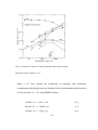
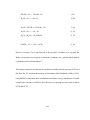
The photofragments produced from photodissociation or photoionization depart with a
fixed amount of kinetic energy (KE) as given in equations (2.1) and (2.2) respectively1:
AB + hv → A + B + KE
(2.1)
AB + hv → AB+ +e- + KE
(2.2)
The kinetic energy is portioned among photofragments according to the conservation of
momentum, as given in equations (2.3) and (2.4):
⎛ M ⎞
KE A = ⎜⎜ B ⎟⎟ × KE
⎝ M AB ⎠
(2.3)
⎛ M ⎞
KE B = ⎜⎜ A ⎟⎟ × KE
⎝ M AB ⎠
(2.4)
According to the mass portioning factor, the lighter particles carry the larger fraction of
kinetic energy. Hence, in a photoionization reaction the electrons carry most of the kinetic
energy, and in the photodissociation of a homonuclear diatomic such as H2 the total
kinetic energy is shared equally between the two H fragments produced.1 According to
conservation of momentum, each photodissociation reaction produces two partner
fragments with equal momentum, flying in the opposite direction of the center-of-mass
frame. These fragments are then able to create scattering patterns with a spherical
distribution known as Newton spheres. For a diatomic molecule with the transition dipole
moment that is aligned parallel to the polarization of the photolysis laser beam, the spatial
distribution of photofragments assumes a cos 2 θ distribution, whereas a sin 2 θ
distribution is produced if the transition dipole moment lies perpendicular to the bond. A
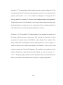
45
single photodissociation event AB + hv → A + B where mass A > mass B creates the
Newton spheres shown in Figure 8. Over time, the photodissociation will produce two
nested spheres with a radii ratio of
RA m A
=
RB m B
(2.5)
where the radius of each sphere is given by
R=
2 KE
t
m
(2.6)
when t is the time-of-flight.
z
Event 2’
θ
Event 1
RA
Event 1’
φ
RB
Event 2
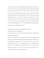
FIG.8. Nested Newton spheres photofragments A and B where mA > mB. The polar angle θ is
defined with respect to the z axis, the azimuthal angle is φ , and the radius is given by R.
Reproduced from Whitaker.1
46
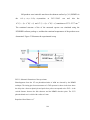
Eppink and Parker13 improved the original technique significantly in terms of
spatial resolution when they replaced the conventional grid electrode assembly used in ion
imaging with a three-plate electrostatic lens with open electrodes. They also introduced an
additional extractor electrode to the ion optics assembly. Additionally, this lens system
could be tuned so that the ions with the same initial velocity are mapped onto the same
point on the detector, regardless of their initial spatial position.13 Hence, this technique of
ion lens optics and 2D imaging became known as “Velocity Map Imaging”.13 and has
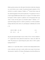
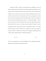
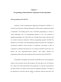
become an essential tool in many different fields. The typical imaging setup includes a
pulsed molecular beam source; an ion optics assembly comprised of repeller, extractor,
and ground electrodes; and an image detector as represented in Figure 9. The images
produced using the ion optics assembly in ion imaging and velocity map imaging are
compared in Figure 10. Furthermore, VMI improves ion imaging by magnifying the radii
of the ion images. Eppink and Parker13 defined this radius (R) as:
R=Nvt
(2.7)
where v is the expansion speed, t is the time-of-flight, and N is a magnification factor that
depends on the experimental setup and electric fields.
47
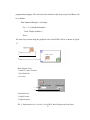
Ion optics
Assembly
Drift Region
Molecular Beam
Detector
CCD
Laser Beam
FIG.9. Schematic representation of the instrument set up in velocity map imaging.
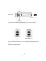
Ion imaging
Velocity map imaging
FIG.10. Comparison between images of O+ ions from the photolysis of molecular oxygen at
225 nm.
Reproduced from Eppink and Parker. 25
48
Chang et al.14 made a significant contribution to the technique by improving the
resolution of the images further. They analyzed each spot detected by the CCD camera
where the burst of electrons created a blur in the image as a result of several pixels being
excited, and eliminated this problem by introducing real-time event counting. The highest
intensity pixel was selected and stored for each ion that struck the phosphor screen, so
that the pixel values correspond directly to the number of ions detected at each pixel
position.11
The raw images from the CCD camera are in fact 3D projections of Newton
spheres on a 2D screen. In order to extract the kinetic energy and angular distribution
information from the images, it is necessary to reconstruct the original 3D distributions.
Suits et al.15 have developed a method by which only the centre slice of the ion sphere is
recorded and thereby circumvents these mathematical reconstruction methods. His DCslicing method is used to stretch the ion sphere (rather than pancaking it) and the detector
is only turned on when the centre fraction of the sphere arrives. This necessitates the use
of additional electrodes and electric fields, but has been widely adopted, especially for
heavier fragments. In addition, there are two fundamental approaches used in literature to
reconstruct the 3D distribution from the projected full ion sphere:15 (a) inversion
methods16 and (b) forward convolution methods.1
The inversion methods assume that if the 3D distribution has an axis of cylindrical
symmetry, and if a 2D-central slice is taken through the 3D distribution, the slice contains
49
all the information required to reconstruct the original distribution.1,16 From this slice, the
3D projection is obtained by rotation around the cylindrical axis – a process known as the
Abel transformation. The inverse Abel transform can be used to obtain the slice from the
projection of the 3D distribution.
In an experimental point of view in a photodissociation process, if the polarization of the
photolysis laser is parallel to the plane of the detector, then the resulting photofragments
will always possess an axis of cylindrical symmetry.1 In such cases, the inverse Abel
transform can be used to recover a central slice from the 3D distribution.1 In cases where
cylindrical symmetry is not observed, forward convolution or basis set methods are
employed.17-19 In the onion-peeling program published by Manzhos and Loock20 , the
velocity and angular distribution is determined by the back simulation of a raw image
with user-defined parameters. Another approach based on Monte-Carlo type simulations
is presented below.
3.1 Experimental Set Up
The velocity map imaging spectrometer consists of a high vacuum chamber, a pulsed
laser system, and a particle detection system. The high vacuum chamber is typically
evacuated to 10-7 Torr. The vacuum system consists of an ionization chamber and a TOF
chamber that are evacuated using two turbo-molecular pump (Pfeiffer, TMU521 and
50
Varian TV701 navigator) backed by Edwards and Welch rotary pumps. The two
chambers are connected by a sliding gate valve.
Gaseous samples are introduced to the vacuum chamber through a molecular beam valve.
The molecular beam is expanded to the vacuum chamber with a cylindrical nozzle and is
collimated by a 0.5 mm skimmer mounted 50-60 mm downstream from the nozzle. The
molecular beam valve is powered by a pulse driver (General Valve, Iota One) that is
synchronized by a LabVIEW program. The gaseous sample is then frozen on to a sapphire
rod (Cryo industries) supported in the middle of the vacuum chamber. The sapphire rod is
attached to a helium compressor (Sumitomo, Cryo Industries HC-4E), and has an Au
(111) plated tip. The temperature of the sapphire rod is controlled in the range 8-120 K by
a temperature controller and a sensor in the cold finger assembly.
Photofragments are produced from the frozen gas sample by laser photolysis of the ice
matrix. They are detected through the (2+1) REMPI process using a second, delayed
probe laser. The probe laser is a tunable and frequency doubled dye laser (Lambda
Physik, Scanmate 2E: Dye Laser) that is pumped by a XeCl Excimer Laser (Lambda
Physik, LPX-200,160-200 mJ/pulse) operating at 308 nm. The output beam from the dye
laser in the probe laser system is frequency doubled using β-BaB2O4 crystal. Photolysis
can be performed using either another dye laser (Lambda Physik, Scanmate 2E) pumped
by an Nd: YAG laser (Continuum Powerlite Precision 8000, 532 nm), or by using an
Optical Parametric Oscillator (OPO) unit pumped by an Nd: YAG laser (Spectra Physics,
51
355 nm). The output of the OPO unit can be tuned between 214-354 nm. The laser beams
are perpendicular to the TOF axis and meet the molecular beam between the repeller and
extractor electrodes.
Infrared spectra will be collected before and throughout the photolysis of the frozen gas
sample with a commercial FT-IR spectrometer (Thermo Scientific Nicolet 6700). The FTIR spectra allow the characterization of the ice matrix. Since FT-IR is used to study the
water ice surfaces, the beam path has to be free of water vapor in the air. This has been
achieved by using an acrylic housing for the beam path that is filled by gas from a purge
gas generator.
The produced photoions are accelerated in a VMI field and drift through a flight tube (74
cm) onto the charged particle detection system. The charged particle detection system
consists of a MCP (Chevron, Burle-Electro Optics Inc.) with a diameter of 75 mm, and a
phosphor screen. Voltages are applied to the MCP to gate-selected ions using highvoltage power supply (Keithley Instruments 245 and 246). The images of the ions that
strike the phosphor screen are detected using a CCD camera (Optikon, 12 bit, 1280 x
1024 resolution) and the images are read out and are stored in the lab computer. The
schematic of the experimental set up is given in Figure 11.
52
Turbo-molecular
FT-IR
pump 1
Cold Tip
OPO
Dye Laser
Dye Laser
Nd: YAG Laser
UV Scan
Nd: YAG
Laser
BBO
Excimer Laser
Turbo-molecular
pump 2
MCP
CCD
FIG.11. Top view of the experimental set up.
53
The studies on physical properties of cryogenic ices, especially related to ice surfaces, the
phase transitions of ice, and the studies of matrix effects on the vibrational spectra of
molecules have received significant attention in the recent years.21-25 However, the
properties of surfaces and the states of the adsorbed species have not been studied
simultaneously. The combination of velocity map imaging to determine the kinetic energy
and the angular distribution of the photoproducts, and FT-IR spectroscopy to determine
the chemical composition of the ice matrix before and throughout photolysis, provide an
optimized method to investigate the photochemistry of water ice and its constituents. The
characteristics of the velocity map imaging spectrometer are important when acquiring the
velocity profile of a photofragment.
In the following section, the characteristics of the velocity map imaging spectrometer are
discussed through a simulation using the Simion 7.0 software package. The dependence
of the resolution on the ion optics voltage is explored through this simulation.
Additionally, a software program written using Microsoft Visual Basic 6.0 to simulate the
experimental pattern observed on the position sensitive detector from the photoproducts is
discussed in detail. These simulations provide useful information for estimates of
resolution for experiments with other photoproducts.
54
3.2 SIMION Simulations
The mapping of the 3D distributions of the desorbed photofragments onto the 2D detector
plane is dependent on the configuration of the electrostatic lens system in the TOF and the
voltages applied to them. The TOF consists of three electrodes, namely repeller (R),
extractor (E) and ground (G). These are used to accelerate the desorbed and resonantly
ionized photofragments into a field-free drift region. Upon ionization, charged particles
form one or several nested Newton spheres which collapse into two dimensions along the
TOF axis for each particular mass.13 In conventional TOF-mass spectrometers, ions of the
same kinetic energy but with velocities in different directions arrive at the detector at
different times. When the velocity map focusing conditions are met, ions of the same
mass that were formed at a given time, with the same velocity, converge on the same
point on the detector, regardless of their position of origin. Since the drift region of the
TOF chamber is of fixed length, the convergence of the beam depends on the ratio of the
voltages applied on the extractor and repeller (VE/VR).
The SIMION 7.0 software package26 allows the calculation of ion trajectories that fly
through 3D electrostatic fields that assume cylindrical symmetry. The SIMION virtual
optics bench was used to simulate the three open-hole electrodes, each 11.4 cm in
diameter, and a TOF chamber that is 74 cm long. The electrode geometries and potentials
at each point in geometry are stored in a potential array, and the voltages applied to the
55
electrodes were then manipulated as required. The modeled spectrometer is given in
Figure 12.
z
y
x
FIG.12. 3D TOF simulated by SIMION 7.0 with repeller, extractor, ground electrodes and
detector.
Five ions of equal mass and without initial kinetic energy were generated in the region
between the repeller and the extractor by first defining the position of the first ion and
then incrementing the position of the others by 1 mm in the y direction, i.e., perpendicular
to the TOF axis. The simulation was repeated for different voltage settings until the
trajectories with the same initial velocity, but different initial positions, were converged to
a single point on the detector. This is the “velocity mapping” condition. The optimal
focusing voltage for VE/VR was found to be 0.55075. After setting the extractor voltage
division “in focus” the setup is ready to collect ion and electron images that do have
56
kinetic energy release.13 If the laser position and VE/VR ratio are kept the same, the only
variable is the repeller voltage (VR) to obtain images in the size that is desired. Now
images of any ion mass can be obtained without having to change the VE/VR ratio.13 This
simulation is illustrated in Figure 13.
R
E
G
Detector
y
x
FIG.13. The xy plane view of the simulated TOF. When VE/VR meets the focusing condition, all
ionized species with the same mass and the same velocity reach the MCP detector regardless of
the location they were formed.
In the next simulation, given in Figure 14, the magnification factor for the image was
calculated. The magnification factor is the factor by which the total image size is larger
than expected, based upon the initial expansion speed and the time of flight.13
57
FIG. 14. The trajectories originate at y=0 mm with one ion ejected with a 90° elevation angle and
other at 0 ° elevation angle.
The empirical relation between magnification factor N, expansion speed v, time of flight t
and the radius R of the ring appearing on the image is described by
R=Nvt
(2.7)
Two ion trajectories originating at the same point with elevation angles of 0° and 90°
were projected onto the detector, and the radius of the ring was obtained. With this
parameter the magnification factor of the image was calculated to be 1.27. The radius of
the image obtained for different voltages applied to the electrodes are given in Table 1.
58
TABLE 1. Results for the radius of the image and magnification factor based on different
voltages applied to the electrodes, using ions with 15 amu mass and 1 eV of kinetic
energy.
VE (Volts)
VR (Volts)
Radius of Image (mm) Magnification Factor
500
275.37
58.33
1.27
750
413.06
41.51
1.27
1000
550.75
36.09
1.27
1250
688.43
32.33
1.28
1500
826.12
29.51
1.28
3.3 Monte-Carlo Image Creation
To simulate an image that is close to the image expected from experiments, a software
program was written in Microsoft Visual Basic 6.0. An 8-bit 512 × 512 pixel image was
obtained by simulating 1,000,000 trajectories with the extractor electrode voltage
calculated from the SIMION simulation, kinetic energy of ions, amplitude of channels,
magnification factor of the image and the anisotropy parameter as inputs.
The photofragments desorbed from the ice matrix will be ionized using the 2+1 REMPI
process and the resulting photofragments are accelerated through the ion optics assembly
before being projected on to the MCP.27 The (y, z) coordinates of the photofragments at
59
the detector can be expressed as follows. This section is related to the back projection
method published by Whitaker.1
z
Z
θ
o
x
O’
φ
y
L
FIG.15. Schematic for the projection of ionized photoproducts (originating at point O) on to the
detector.
As shown in Figure 15, the point of origin of the photofragments, which corresponds to
the REMPI ionization region, is defined as origin (x = y = z =0). The initial velocity
distribution of the photofragments can be written using spherical polar coordinates θ , φ
and the initial velocity v0 as:
vo x = v0 sin θ cos φ
voy = v0 sin θ sin φ
(2.8)
voz = v0 cos θ
60
The ionized fragments will then be accelerated through a homogenous electric field E,
along the TOF axis Ox with a force of
Fx = Eq
(2.9)
where q is the elementary charge.
The co-ordinates (x, z) at the detector are calculated as
y=
z=
2 L cos φ sin θ
ρ
2 L cos θ
ρ
( sin φ sin θ + ρ − sin φ sin θ )
2
2
( sin φ sin θ + ρ − sin φ sin θ )
2
2
(2.10)
(2.11)
where ρ is the ratio between electrostatic energy acquired in the field and the initial
kinetic energy in the particle
ρ=
qEL
1 2
mvo
2
(2.12)
and L is the distance between the region where the desorbed products are ionized and
detected.
Since the initial kinetic energy of the desorbed products are estimated to be less than 1
eV, and since the kinetic energy gained through the accelerating field is extremely large,
the equations for positions (y, z) are reduced to:
y=
2L cos φ sin θ
(2.13)
ρ
61
z=
2L cos θ
(2.14)
ρ
The fragments from photodissociation are ejected parallel or perpendicular to the
polarization direction of the light with an angular distribution given by
I (θ ) = (1 + β P2 (cos θ ) ) / 4π
(2.15)
where θ is the angle between the fragment velocity vector and light polarization direction,
and P2 (x ) = (3x 2 − 1) / 2 is the second-order Legendre polynomial. The (y,z) co-ordinates
are calculated by the Visual Basic program as stated below. The program generates three
random numbers, R1, R2 and R3, which are distributed evenly between zero and one. From
R3 one can calculate φ = 2πR3 . However, θ is not calculated directly as θ = πR2 in the
program, since even for an isotropic distribution this equation would bias towards
intensity at the “poles” of the image. For an anisotropic distribution the intensity is given
by equation (2.15).
Using a random number generator it is possible to construct random numbers taken from
a variety of distributions. If there are equal distributions of random numbers R1, R2 and R3
the random number generator can be used to generate the numbers. If the random
numbers are of a linear distribution, they can be generated by the von Neumann
algorithm. The von Neumann algorithm generates non-linearly distributed random
numbers using a biased condition statement as follows.
62
This algorithm generates an even distribution of random numbers in the range (x1, x3).
To generate a random number R uniformly on (x1, x2) assuming we can generate randomly
on the range (x1, x3).
x1
x2
x3
To generate a linearly distributed array of random numbers the algorithm is modified to
(a) Generate R1 uniformly on (x1, x3) and generate R2 uniformly on (x1, x3)
(b) If R1< R2 then take R1 as the random number on the distribution
(c) If not, go to (a).
The expression for θ is still more complicated and given in (2.15). We can then generate
the random angular distribution in θ from:
(a) generate R1 uniformly on (x1, x3) and generate R2 uniformly on (x1, x3)
(b) if ( β 2 × 0.5 × (3 × Cos(R1 × π ) 2 – 1)+1) < R2 then take R1 as the random number
on the distribution. The angle θ = arcos (R2).
(c) if not, go to (a).
If the value obtained from the conditional statement is greater than R2, then the value is
kept without being discarded. The Visual Basic program therefore contained the
following code:
63
If ( β 2 × 0.5 × (3 × Cos(R1 × π ) 2 – 1)+1) / (1 - β 2 × (-0.25 - Sgn( β 2 × 0.75))) > R2
Then
θ = arccos(R1)
φ = 2πR3
Y =
Z =
2 LCos (φ ) Sinθ
ρ
2 LCos (θ )
ρ
The expression (1 - β 2 × (-0.25 - Sgn( β 2 × 0.75))) is a normalization factor for the
anisotropy parameter. In Visual Basic the “Sgn” function returns an integer that indicates
the sign of the operation. The Visual Basic code has been included in the appendix
section.
The calculated co-ordinates of each ion are stored in an array. An image is calculated as
counts of the number of events falling within each pixel. The code given below illustrates
how binning into an image with a resolution of res × res pixels, can be used to increase
the intensity of the pixels if two ions with the same co-ordinates are generated in a binned
image. Rmax is the maximum radius of the image.
Yimage = Int((Y / Rmax + 1) * res / 2
Zimage = Int((Z / Rmax + 1) * res / 2
IntImage(Yimage, Zimage) = IntImage(Yimage, Zimage) + 1
64
To verify that the simulation code actually works, the 3D simulated image was then
inverted with the onion-peeling program20 to obtain a 2D slice through the center of the
image. The 2D image provides information about velocity profiles and spatial anisotropy
parameters and is expected to recover the input parameters from the simulation.
The program calculates angular distribution at a given radius. The angular distributions
resulting from an ionization process can be expressed as a sum over Legendre polynomial
components:
N
I (θ ) = c ∑ β n Pn (cos θ )
(2.16)
n =0
Where N depends on the number of photons driving the process, and θ is the angle
between the axis of polarization of the photolysis light and the velocity of the fragments.
If the normalization coefficient c is chosen so that β 0 = 1 , the remaining coefficients β n
are known as the spatial anisotropy parameters. 20
The onion-peeling program transforms the image from Cartesian coordinates to polar
coordinates28-30, and by fitting the angular distribution to the above function and the
anisotropy parameter , β 2 is determined for each radius.
The values for the spatial anisotropy parameters that were used to construct the simulation
and those recovered from the onion-peeling program and the Abel transform were then
65
compared. A discrepancy between the simulation input and the output were observed
because the velocity distributions are set very narrow during the inversion process and
that throws off the program. Therefore the simulation was repeated with velocity
broadened distributions and the spatial anisotropy parameters were recovered. The results
are given in Table 2 while the inverted images are given in Figure 16.
66
Simulated Image from the
Visual Basic Program
Inverted Image from the
Onion Peeling Program
Inverted Image from the Abel
transform
FIG.16. Typical image simulated by the Visual Basic program (top) using broadened velocity
distributions, the Inverted image from the Onion Peeling Program (middle), and the Inverted
image from the Abel Transform (bottom).
67
TABLE 2. Anisotropy parameters for simulated image and inverted image from the
velocity broadened distribution.
β 2 used for the
simulation
β 2 recovered
from the Onion Peeling
Program
β 2 recovered
from the Abel transform
1.8
1.77
1.82
-1
-1.03
-0.94
0
0.08
0.1
0.5
0.5
0.5
-0.5
-0.51
-0.52
3.4 Conclusion
A significant amount of information about the ice matrix and the desorbed species from
the ice surface can be extracted by combining the REMPI spectroscopy and FT-IR
spectroscopy. In this section, the principle of the velocity map imaging spectrometer has
been discussed, together with the inversion procedure to extract physical information
from the acquired images. Resolution characteristics of the velocity map imaging
spectrometer have been investigated with the ion trajectories simulation using Simion 7.0
software package. The results from this simulation provided an understanding of the
voltages that can be applied to the ion optics assembly to optimize the resolution of the
68
experimental image of photoproducts. With the Visual Basic program discussed in this
section, it is possible to simulate the images of the desorbed species from the ice surface.
However, the expected image would be a semi-circle, as desorbed species are only
directed to the space above the cold tip. These simulations will aid in acquiring the
velocity profile of the photoproducts, and provide more accurate energy distributions to
propose mechanisms for reactions in water ice and its constituents.
69
References for Chapter 3
1
B. J. Whitaker, Imaging in Molecular Dynamics (Cambridge University Press,
Cambridge, 2003).
2
B. J. Whitaker, Image Reconstruction: The Abel Transform, in: A. G. Suits, R. E.
Continetti (Eds.), ACS Symposium Series, Vol. 68, Oxford University Press, 2000.
3
A. Heck, Europ. Mass. Sectr. 3, 171 (1997).
4
P. L. Houston, Acc. Chem. Res. 28, 458 (1995).
5
P. L. Houston, J. Phys. Chem. 100, 12757 (1996).
6
S. H. Lee, H. I. Lee, and Y. T. Lee, J. Chem. Phys. 121, 11053 (2004).
7
J. Solomon, J. Chem. Phys. 47, 889 (1967).
8
D. W. Chandler, and P. L. Houstan, J. Chem. Phys. 87, 1445 (1987).
9
W. C. Wiley, I. H. McLaren, Rev. Sci. Instrum. 26, 1150 (1955).
10
A. J. R. Heck, and D. W. Chandler, Annu. Rev. Phys. Chem. 46, 335 (1995).
11
C. Vallance, Philos. Trans. R. Soc. London, A, 362, 2591 (2004).
12
D. M. Sonnefroh, and K. Liu, Chem. Phys. Lett. 176, 183 (1991).
13
A. T. J. B. Eppink, and D. H. Parker, Rev. Sci. Instrum. 68, 9 (1997).
14
B. Y. Chang, R. C. Hoetzlein, J. A. Mueller, J. D. Geiser, and P. L. Houston, Rev. Sci.
Instrum. 69, 1665 (1998).
15
A. S. Bracker, E. R. Wouters, A. G. Suits, and O. S. Vasyutinskii, J. Chem. Phys. 110,
14 (1999).
16
G. A. Gracia, L. Nahon, and I. Powis, Rev. Sci. Instrum. 75, 4989 (2004).
70
17
C. Bordas, F. Pauling, H. Helm, and D. L. Huestis, Rev. Sci. Instrum. 67, 6 (1996).
18
M. J. Bass, M. Brouard, A. P. Clark, and C. Vallence, J. Chem. Phys. 117, 19 (2002).
19
M. J. Bass, M. Brouard, A. P. Clark, B. Martinez-Haya, and C. Vallence, Phys. Chem.
Chem. Phys. 5, 856 (2003).
20
S. Manzhos and H.-P. Loock, Comp. Phys. Commun.,154, 76(2003).
21
R. H. Brown and D. P. Cruikshank, Annu. Rev. Earth Planet Sci. 25, 243 (1997).
22
J. E. Schaff and J. T. Roberts, J. Phys. Chem. 100, 14151 (1996).
23
A. Susa and S. Koda, Meas. Sci. Technol. 15, 1230 (2004).
24
S. Malyk, G. Kumi, H. Reisler, and C. Witting, J. Phys. Chem. 111, 13365 (2007).
25
D. L. Cocke, J. A. G. Gomes, J. L. Gossage, K. Li, C.-J. Lin, S. Tandel, App. Spec. 58,
528 (2004).
26
D. A. Dahl, J. E. Delmore, and A. D. Appelhans, Rev. Sci. Instrum. 61, 607 (1990).
27
C. Romanescu, S. Manzhos, D. Boldovsky, J. Clarke, H.-P. Loock, J. Chem. Phys., 120,
767 (2004).
28
J. Winterhalter, D. Maier, J. Honerkamp, V. Schyja, and H. Helm, H. J. Chem. Phys.,
110, 11187 (1999).
29
V. Dribinski, A. Ossadtchi, V. A. Mandelshtam, and H. Reisler, Rev. Sci. Instrum. 73,
2634 (2002).
30
O. Ghafur, W. Siu, P. Johnson, M. F. Kling, M. Drescher, and M. J. J. Vrakking, Rev.
Sci. Instrum. 80, 033110 (2009).
71
Chapter 4
Programming of Instrumental Components in the Experiment
4.0 Programming with LabVIEW
Laboratory Virtual Instrumentation Engineering Workbench (LabVIEW) is a
powerful tool developed by National Instruments (NI) that enables computerized control
of instruments. The building blocks used in LabVIEW programming are known as
Virtual Instruments (VIs). The programming approach in VIs is the utilization of
graphical programming code, which makes use of graphs, charts, gauges, and meters that
are created to emulate an instrument.1 With this programming approach LabVIEW has
introduced a user-friendly visual programming technique that allows the controlling of
experimental conditions, remote operation of instruments, and analysis of data. In
comparison to traditional instruments, the VIs created in LabVIEW provide more userdefined and more application-oriented solutions.1 This chapter illustrates the
programming of the instrumental components of the experiment using LabVIEW 8.6.
The graphical development environment in LabVIEW has two main components,
which are the front panel and the block diagram. The front panel is the User Interface
(UI), which is the visual representation of the application. It is typically characterized by
the knobs, buttons, and controls which emulate the traditional instrument.1 The inputs to
the application are provided, and the outputs are displayed using the front panel. The
72
block diagram contains the graphical source code and reflects a flow chart rather than the
usual lines of code seen in computer programs. LabVIEW supports modularity and
breaks down tasks to manageable sub-tasks, such as nodes and sub-VIs. Nodes in
LabVIEW represent functions, operators, and subroutines in standard programming
languages.1 Structures are type of nodes that are commonly used in LabVIEW to execute
code repeatedly or conditionally. They are comparable to the loops, conditional
statements, and case structures used in text-based programming. These nodes and subVIs can also make use of the libraries available for the instrument. Terminals in the block
diagram serve as entry and exit points for data between the front panel and the block
diagram. The terminals, nodes, and sub-VIs are connected to each other to perform a task,
using virtual wire connections. Wires serve as data paths between source and destination
terminals. They are comparable to variables in text-based programming languages.1 In
text-based programming languages, different data types are used to eliminate the
confusion of variables. LabVIEW implements the same principle in graphical
programming by using different colors and styles in its wiring.1 Hence, the block diagram
is a visual representation of the inputs, functions, sub-VIs, wired connections, and
outputs. The functionality of a LabVIEW program in comparison to a text-based program
is illustrated in the following example. Let us suppose that a user would like to specify
the number of measurements he wants from a certain device, and would like to see how
many measurements the device has taken while he is running the experiment. This
repetitive cycle of measurements can be implemented using a “for loop” in a standard
73
programming language. The text based code written for this loop using Visual Basic will
be as follows:
Dim NumberOfSamples, i As Integer
For i = 1 To NumberOfSamples
Print "Display Number", i
Next i
The same loop written using the graphical code in LabVIEW will be as shown in Figure
17.
1
Display
Count Number
2
3
Block Diagram Icons:
1- Numeric Control Terminal
2- Wire Data Path
3- For Loop
1
2
Front Panel Icons:
1- Digital Control
2- Digital Indicator
FIG.17. Implementation of a “for loop” in LabVIEW- Block Diagram and Front Panel.
74
The principle followed in the source code of the LabVIEW program is similar to the textbased programming languages. However, LabVIEW is advantageous in terms of not
having to declare or initialize variables as opposed to most programming languages. An
additional advantage is that LabVIEW simultaneously creates the front panel as the
programming on the block diagram takes places.1
LabVIEW also allows the utilization of built-in tools such as Measurements Automation
Explorer for programming the Data Acquisition Devices (DAQ). The standard I/O
language for instrumentation programming is Virtual Instrumentation Software
Architecture (VISA). VISA is a capable of controlling General Purpose Interface Bus
(GPIB) and serial instruments, and call lower level drivers.1 VISA resources, operations,
and attributes commonly used in LabVIEW programming. The VI communicates with a
device by establishing a VISA session. The basics of this process are used in LabVIEW
programming as shown in Figure 18.
Open Session
Write
Close Session
FIG.18. Communicating with an instrument.
75
Report Error
The instrument I/O tools in LabVIEW create the components required to communicate
with an external device attached to a serial or a GPIB port and provides the ability to
switch between interfaces.
This chapter discusses the programming of the instruments used in the experiment
by using LabVIEW 8.6. The experimental details of velocity map imaging have been
discussed in detail in chapter 3. An overview of the experimental section will be
presented in the following section in light of the programming process.
The main elements of the programming environment are a pulsed laser system, a
Molecular Beam Valve (MBV), and a charged particle detection system. The pulsed laser
system is comprised of a photolysis laser (Lambda Physik, LPX200, Excimer Laser) and
a probe laser (Scanmate, Lambda Physik, Dye Laser) pumped by a Nd:YAG Laser
(Continuum). The timing of the photolysis and probe lasers is achieved through a delay
generator (DG 535, Stanford Research Systems) and a PCI6602 timing board via the
DG535 VI and the PCI6602 VI. The latter is used to control the MBV as well. The ions
generated in the vacuum chamber are accelerated through an ion optics assembly and
pass through a time-of-flight (TOF) region before hitting the MCP. The high voltage
applied to the ion optics assembly and the MCP (Chevron configuration, Burle ElectroOptics, Inc) is controlled by the PS350 High Voltage Power Supply VI. The MCP is gated
with a high voltage pulse to allow only ions of interest to be detected. The TOF profile of
these ions is observed through a digital oscilloscope (Tektronix, DPO3034 series) and
76
recorded as a function of the probe laser wavelength via the Stepper Motor Scope REMPI
VI. The cascade of electrons that strike the phosphor screen creates an ion image which is
recorded by a CCD camera (Sensicam, Optikon, 12 bit, 1280 x 1024 resolution)
controlled by the Imaging VI. Figure 19 shows the layout of the VIs for data acquisition.
77
Nd:YAG
Laser
Fig.19. Schematic for the data acquisition system using VIs.
78
4.1 PS 350 series High Voltage Power Supply
The four PS 350 series High Voltage Power Supplies are used to control the
voltages applied to the repeller plate, back MCP, extractor plate, and the phosphor screen.
The PS 350 series High Voltage Power Supply is remotely manipulated by the Lab
VIEW program via the GPIB interface. In order to communicate with the GPIB interface,
the address of the PS 350 device must be configured. This is achieved by selecting the
appropriate GPIB name from the VISA resource drop-down menu. The VISA resource
name is unique to an instrument I/O session. It specifies which device to communicate
with and all the configuration information to perform the I/O. This prompts the opening
of a session with the selected device specified by the VISA resource name and the
program returns a session identifier that can be used to call any other operations in the
power supply. This process is shown in Figure 2.
FIG.20. Communication with the device.
79
The front panel in Figure 21 allows the user to specify the exact voltages required
using the “start” and “end” controls. The ability to change the voltage in small increments
is important to prevent damage to the assembly, and also to observe the changes in the
image when the repeller and extractor voltages are adjusted. The “step” and
“increase/decrease” controls allow this manipulation. The output voltage is displayed in
the “VCurrent” box. The output voltage cannot be set higher than the voltage limit.1
FIG.21. Front panel of power supply.
80
In addition, if the output exceeds 10% of the full scale, the unit trips and the high
voltage is disabled. If this occurs, a ‘VTRP’ (voltage trip) message appears in the panel.
The “Source Setting” sliding switch allows the user to specify the source before setting
up its limit. The default has been set to voltage and the switch manipulates the voltage
setting, provided that the front panel switch is turned on the instrument. If the switch is in
the OFF position while trying to set the high voltage, the high voltage is left off and an
execution error is reported. The “Enable Voltage Inversion” control changes the voltage
from positive to negative. All of the above-mentioned inputs are directed to the VISA
Write Function in LabVIEW and the data is then written into the device.
4.2 DG 535 Digital Delay and Pulse Generator
The DG 535 can produce four digitally controlled time intervals. These time
intervals can be controlled by using a LabVIEW program through the GPIB connector.
The IEEE-488.2 connector allows the computer to control the DG 535. The DG 535
consists of five delay out BNCs named T0, A, B, C, and D.5 T0 sets the start time for the
timing interval when the DG 535 receives a pulse from the master trigger. The LabVIEW
program allows the manipulation of the delays in the channels A, B, C, and D. The delay
outputs A, B, C, and D can then be set with respect to T0 or each other from 0 to 1000 s
with increments of 5 ps. 5 For example, the delay menu can be set as:
81
A = T0+ 4 ns
B = A + 5 ns
C = T0+ 2 μs
D=C+0
where channel A is referenced to T0 and channel B is set to A’s delay plus 5 ns. This
allows the program to specify the start time and the pulse width. The program allows the
user to control the each channel through the “Time Base Menu” in the front panel and the
“Delay Menu.”
The DG 535 can be triggered internally or externally. The external trigger port on
the DG 535 is connected to the Excimer laser (Lambda Physik LPX 200i). The four pulse
outputs are labeled A∪B, A∩B, C∪D, and C∩D. The pulse output A∩B is connected to
the high voltage gate and A∪B displays the same pulse on the oscilloscope. The pulse
output C∪D is connected to the “Trig-in” port for the CCD camera on the computer, in
order to control the CCD exposure time and C∩D displays the same pulse on the
oscilloscope. The front panel of the DG535 VI is shown in Figure 22.
82
FIG.22. DG 535 front panel.
The front panel allows the internal trigger mode to be manipulated by setting the trigger
rate; the external trigger mode can be controlled by specifying the threshold trigger level,
slope and termination impedance of the external trigger input. The burst mode can be
controlled by specifying the trigger rate, the burst period, and number of pulses per burst.
83
4.3 Data Acquisition with LabVIEW
The primary Data Acquisition (DAQ) processes used in this section generate signals,
analysis, and presentations on the computer.2 This process is implemented by utilizing the
main components of DAQ which are data signals, DAQ hardware and driver
applications.2 Using these components, it is possible to use counters and timers to
generate pulses and pulse trains with LabVIEW. Virtual channels for data acquisition,
triggering and synchronization can be created with LabVIEW palettes and Sub-VIs.
4.3.1 Triggering
The triggering of events in data acquisition can occur in three possible ways:1
1. External triggering
2. Internal triggering
3. Software-generated triggering
External triggering occurs when an interface uses digital pulses from specialized
hardware or equipment to synchronize events. Internal triggering is common in DAQ
devices and occurs when an inbuilt-comparator detects the signal crossing of a specified
signal level and in turn triggers an event.1 In software-generated triggering, a software
program is responsible for the occurrence of event such as data acquisition.
In this section, a LabVIEW program is used for data acquisition through NI-PCI 6602E
card which is plugged into a computer through a connector block (CB-68LP). NI-PCI
84
counter / timer devices can be easily used across multiple hardware devices as they are
equipped with a Real Time System Integration (RTSI) bus line.1
4.3.2 Triggering with PCI 6602E VI
This VI has been written using the DAQ features in order to synchronize
instrument components in the experiment such as the Nd : YAG laser, Delay Generator,
and Pulsed Valve. The synchronization process is performed by the “Master Device” and
“Slave Device” panels seen in the front panel of the VI. Hardware synchronization is
achieved through the RTSI cable, which is a high-speed digital bus that exchanges timing
signals between NI boards. In the LabVIEW programming environment, the NI-DAQ
driver is responsible for routing and driving the RTSI bus automatically via the Route
Signal VI. The LabVIEW program written for the PCI-6602 makes use of this feature by
generating a pulse in counter 0 and then translating that pulse to all the counters through
the RTSI bus, thereby synchronizing the connected devices.2,6
The pulse for the master device was programmed by using the classes of the DAQ
Create Virtual Channel. The numerous classes of the DAQ Create Virtual Channel are
able to perform functions such as temperature measurement, voltage generation, event
counting, and corresponding with I/O channels.1 The instance of this channel employed
in programming PCI 6602 is “CO Pulse Time.” The CO Pulse Time Channel creates a
digital pulse defined by the pulse width and initial delay specified by the user. The initial
85
state of the pulse was defined as “low.”3 The basic implementation of DAQ features to
generate a pulse is shown in Figure 23.
FIG.23. DAQ in the PCI 6602E VI.
4.3.2.1 Implementation of the PCI 6602E VI
The input “task in” is then provided to the Timing Implicit VI, which in turn,
configures the duration of the pulse generation and the number of pulses to generate.2 The
Export Signal VI then routes the control signal to the terminal specified by the user.3 The
Start VI initiates pulse generation, and the Is Task Done VI queries the status of the task
and indicates the completion of the execution cycle.3 Once the execution cycle has been
86
completed, the Clear Task VI stops the task, releases the resources reserved, and clears
the task.3
Similarly, the digital pulses for all the slave devices are generated by the CO Pulse Time
Channel. The I/O counter denotes the names of the counters to create the virtual channels.
The DAQmx physical channel constant provides all the counters and devices installed in
the system, and they can be selected from the drop-down menu in the front panel.3
4.3.2.2 Front Panel of the PCI 6602E VI
The front panel is comprised of two main panels for master and slave devices as
shown in Figure 24. In the master device panel, the user is able to input the amount of
time the pulse must be high, and the amount of time (in seconds) to wait before
generating the first pulse by using the digital controls for “width” and “initial delay”,
respectively. The initial delay in the master device is defined as T0.
87
FIG.24. Front Panel of PCI 6602 VI.
In the slave device panel, the counters 1-4 have been assigned to the following devices:
Counter 1 – Nd: YAG laser flash lamp
Counter 2 – Nd: YAG laser Q switch
Counter 3 – DG 535
Counter 4 – Pulsed Valve
88
The names of the counters for each of the devices can be selected from the DAQphysical-channel-constants drop-down menu. The user is also able to specify the pulse
width and initial delay for each counter using the respective digital controls. The time
base indicator displays the reference for the delay in each counter. The default setting for
the time base indicator in all the counters has been set to T0. However, the user is able to
change this reference using the time base digital indicator. The delay indicator displays
the calculated total delay for each counter based on the initial delay and time base. The
delay is set with reference to the rising edge from the pulse in counter 0. Total delay for
each counter is displayed in the “Show Relative Delay” wave graph. Any errors that
occur during operation will be displayed in the “Error out” panel.
4.4 Collecting TOF and REMPI spectra using LabVIEW
The following section discusses details of the VI written to collect TOF and
REMPI spectra. The TOF spectra were collected using an oscilloscope and were
transferred to the computer for analysis. The REMPI spectrum for each species is then
calculated from the TOF spectrum. Since the TOF profiles are recorded as a function of
the probe laser wavelength, a stepper motor unit was utilized to manipulate the probe
laser wavelength using the computer. Hence, the VI described in this section has three
panels:
89
1. Stepper motor panel to control probe laser
2. Oscilloscope panel to store TOF spectra
3. TOF and REMPI spectra panels
Each of these components will be discussed in the following section.
4.4.1 Stepper motor panel to control probe laser
The ability to control the probe laser wavelength is important in aligning the
probe laser and when collecting the TOF spectrum. This is achieved through a stepper
motor (NEMA 17 Unipolar) that controls the grating of the laser. The stepper motor, in
turn, is controlled via a data acquisition device (Measurements Computing, USB1208FS)
that triggers the stepper motor driver (QK179). These devices are shown in Figure 25.
FIG.25. Stepper motor controller and data acquisition device.
90
4.4.1.1 Implementation of the stepper motor controller
The address of the driver port and the direction of rotation in the stepper motor
have been configured using VIs for the data acquisition device from Measurements
Computing, as given in Figure 11. These VIs allow the port to be configured as an output
port and to set the direction bit. The stepper motor program can be used from a standalone VI to align the probe laser or from the QK179 panel on the Stepper Motor Scope
REMPI VI to collect TOF spectra.
FIG.26. Block diagram to change direction of rotation in the stepper motor.
4.4.1.2 Front panel of the stepper motor controller
The front panel of the sub VI is given in Figure 27. In it the user can specify the
direction of rotation for the motor and the start wavelength. The default settings for the
pulse width have been set to 5, the delay has been set to 0, and the number of steps per
91
loop has been set to 200. Upon execution, the current wavelength of the probe laser will
be indicated in the panel.
FIG.27. Front Panel of the Stepper motor sub VI.
4.4.2 Oscilloscope panel to store TOF spectra
4.4.1.3 Front panel of the oscilloscope
The TOF spectrum is observed in the digital phosphor oscilloscope as shown in
Figure 28. The “Remote Control” button starts the execution of the DPO3034 panel. The
VISA resource name of the oscilloscope can be selected from the drop-down menu. By
specifying the VISA resource name, the user allows the computer to acquire data from
the oscilloscope through the USB cable.7 The digital control for channels allows the user
to display the waveform in the desired channel. The “Maximum Time” control specifies
92
the amount of time to wait for the acquisition of data. The default is set to 10000 ms. The
“Save” button saves the spectrum into the path specified by the user.
4.4.1.4 Implementation of the oscilloscope
The DPO3034 panel has been programmed with the following sequence of
operations: Initializing the session with the instrument; sequentially acquiring data;
waiting until the operation is complete; acquiring the waveform; and closing the session.7
The Single Waveform VI initiates acquisition based on the configuration information,
waits for the acquisition to complete, and returns the requested waveform. The Close VI
runs an instrument error query before closing the session.3,10
FIG.28. Front panel of the Stepper Motor Scope REMPI VI.
93
4.4.3 TOF and REMPI spectra panels
When the voltage applied to the MCP exceeds 1500 V, the MCP turns into the
gain mode and can be used to gate ions of interest.8,9 The TOF profiles are used to record
ions as a function of wavelength of the probe laser. The TOF spectrum is then exported
from the oscilloscope to the computer using the DPO3034 sub-VI and is displayed in the
“Waveform” graph on the front panel in the Stepper Motor Scope REMPI VI. The
waveform graph has a pair of horizontal cursors and four vertical cursor units. Each
vertical cursor unit is comprised of a start and end cursor. In order to form the REMPI
spectrum, the user must select the desired peak for analysis by positioning the cursors.
The execution of this program can be initialized by the “REMPI Collect” button. The
REMPI spectrum is produced by calculating the area of the TOF peaks of interest as a
function of wavelength. The REMPI spectrum will then be displayed in the “REMPI
Waveform” panel, and the spectrum can be saved to a user-specified location with the
“REMPI save” button.
4.5 Imaging VI
The SensiCam system consists of two major components, which are the PCI
interface board and the camera head.11 LabVIEW communicates with the PCI interface
board by using the SENNTPCI.DLL libraries. The PCI board communicates with the
camera through a high-speed serial link. Camera control is performed by sending the
94
Camera Operation Code (COC) to the camera head.12 Once the COC is uploaded to the
camera head, exposure commences. COC will specify the parameters required to create
an exposure. These parameters include trigger mode, delay from trigger to start exposure,
region of interest, and binning. These parameters are included in the front panel of the
Imaging VI.12 The procedure used in this VI is as follows:
ƒ
Initialize the camera
ƒ
Upload the COC
ƒ
Start the exposure
ƒ
Wait until exposure terminates
ƒ
Retrieve imaging data
The front panel allows the user to specify the board number, run mode, mode of
operation, and the read out mode. The board number inputs the board ID to the VI, the
run mode controls single or continuous trigger exposure, the mode of operation initializes
the code, and the read out mode specifies if the read out is upright or inverted. The CCD
temperature should be approximately -13˚C and the temperature of the electronics should
be maintained at 33˚C. These temperatures are displayed on the respective thermometers
on the front panel.
The camera controls panel allows the user to specify the programmable controls.
The “Camera Type” digital control allows the user to select the model of the camera
connected. The choice of the camera model determines the behavior of the other
95
parameters. “Horizontal binning” combines pixels horizontally and “Vertical binning”
combines pixels vertically for increased sensitivity. The four digital controls of ROI Left,
ROI Right, ROI Top, and ROI Bottom specify the region of interest.
The camera information panel displays the specifications such as resolution, camera ID,
CCD type, and temperature control. The image size status is used to display error codes
along with the error out panel. The horizontal and vertical size indicators display the
number of pixels in the image. The “image grab” can be used to save data to a user
specified location.
The “Image 12 bit” panel shows each image shot at any given time, the “Count 12 bit”
panel shows the sum of several shots, and the “Image 16 bit” panel scales the 0-4096
grayscale values of the 12 bit images up to 0-65535 and displays it as a 16 bit file. The
front panel for the Imaging VI is given in Figures 29 and 30.
4.5.1 Implementation of the Imaging VI
The Imaging VI has been programmed using several sub VIs made for SensiCam.12 For
example, the SCSetBoard VI controls the communication with the board, SCSetMode VI
sets the mode of operation for subsequent camera function calls, the SCGetStatus VI
interrogates the camera for configuration and temperature information, and the
SCGetImageSize VI determines the number of horizontal and vertical pixels in the current
96
image configuration. The scaling of the 12 bit image to a 16 bit image and normalizing it,
has been implemented using a two dimensional array. Part of the block diagram is shown
in Figure 31.
FIG.29. Imaging VI, front panel 1 for user inputs.
FIG.30. Imaging VI, front panel 2 to display images.
97
FIG.31. Imaging VI, block diagram.
4.6 Conclusion
The synchronization of the elements in the apparatus is important in the experimental
procedure. This has been achieved by the virtual instruments created using LabVIEW
8.6.The programs written allow the user to set the experimental parameters, and collect
data using the data acquisition system. Since the programs support modularity, it is also
possible to add other components to the same programs in the future without disrupting
the existing modules.
98
References for Chapter 4
1
S. Sumathi and P. Surekha, LabVIEW based advanced instrumentation systems,
Springer (2007).
2
http://www.ni.com
3
LabVIEW help menu
4
Stanford Research Systems, Series PS 300, User Manual (1998).
5
Stanford Research Systems, DG 525, User Manual (1999).
6
National Instruments, DAQ 6023E/6024E/6025E, User Manual, January (1999).
7
MSO3000 and DPO3000 Series Digital Phosphor Oscilloscopes User Manual, Tektronix
8
D. M. Bolodovsky, Photodissociation dynamics of bromine chloride probed by velocity
map imaging, M. Sc. thesis, Queen’s University (2006).
9
C. Romanescu, Velocity imaging of the photodissociation and photoionization dynamics
of hydrogen chloride and hydrogen bromide, Ph. D. thesis, Queen’s University (2007).
10
C. Elliott, V. Vijayakumar, W. Zink, and R. Hansen, National Instrument LabVIEW: A
programming environment for laboratory automation and measurement, The association
for Laboratory Automation, (2007).
11
SensiCam Optikon, Operating Instructions (1999).
12
LabVIEW drivers for Sensicam Version 3.0.
99
Chapter 5
Photolysis of Amorphous Solid Methanol at 157 nm
5.0 Background
During the period from November 2008 – December 2008 I had the opportunity to work
with Prof. Masahiro Kawasaki’s research group in Kyoto University, Japan under an
Ontario Centre for Excellence fellowship. During this period I became involved in
experiments on the photochemistry of methanol ice as part of the preliminary
experiments required for the development of the VMI apparatus at Queen’s University.
Upon my return I was able to perform simulations of the photofragments using
PGOPHER software (by C. M. Western, University of Bristol) with the help of
postdoctoral fellow, Wei Guo. This chapter is based on the experiments performed in
Kyoto. The figures used in the experimental and results sections in this chapter have been
reproduced from a publication co-authored by my collaborators and myself.
5.1 Introduction
Interstellar dust grains, with ice mantles coating their surface are rich with numerous
chemical compounds such as H2O, NH3, CH4, O2, N2, CO, CO2 and H2CO. As interstellar
dust grains are continuously exposed to a low flux of UV photons, molecular bonds are
broken within femtoseconds and the photofragments recombine, giving rise to complex
100
molecules. The production pathways of such molecules have been of great astrophysical
interest.1–4
Methanol is also known to be a primordial constituent found abundantly on the icy
mantle of dust grains, comets and other solar bodies.2 Mumma et al.5 reported that the
abundance of methanol in Oort cloud comets is 1 – 3% relative to water. The
photochemistry of the methanol–rich interstellar medium is expected to form large
organic molecules.
Various dissociation mechanisms at 157 nm for methanol in the gas phase have been
reported.6,7 Lee et al.8 suggested that the detected photoproducts were formed through the
channels given in reactions (3.1–3.5) and that secondary dissociation occurs from CH3O
and H2CO.
CH3OH + hυ → CH3O + H
(3.1)
CH3OH + hυ → H2CO + 2H
(3.2)
CH3OH + hυ → H2CO + H2
(3.3)
CH3OH + hυ → CO+ 2H2
(3.4)
CH3OH + hυ → CH3 + OH
(3.5)
101
Satyapal et al.9 investigated the possible bond cleavage in gas phase methanol at 157 nm
and reported that the O–H cleavage channel through reaction (3.1) was dominant with a
quantum yield of (0.86 ± 0.1). The remainder was thought to be through the C–O
cleavage channel via reaction (3.5). However, this contribution had not been quantified.1
The photodissociation of solid methanol is more complex than in the gaseous phase since
the photofragments are trapped in the site of production. Hence, the photochemistry of
solid methanol has received much attention during the recent years.
Gerakines et al.2 have studied the UV photochemistry of pure methanol ice samples at 10
K through infrared absorption spectroscopy. They reported the formation of carbon
monoxide (CO), methyl formate (H3COHCO), carbon dioxide (CO2), methane (CH4),
formyl radical (HCO), formaldehyde (H2CO), and hydrogen (H2), as given in Figure 32,
which was indicative of a complex photochemistry for methanol.1,2 However, they could
not detect the primary CH3 and OH fragments. The possible reaction pathways for the
products obtained from photodissociated solid methanol are given in reactions (3.6 –
3.14).1,2,4 The primary photo products from the photodissociation of solid methanol may
further react with the solid methanol matrix to produce secondary photoproducts.
102
FIG.32. Evolution of features in CH3OH irradiation. MF= methyl formate.
Reproduced from Gerakines et al.2
Hama et al.10 have reported the mechanisms for hydrogen atom abstraction,
recombination and hydrogen molecule elimination from solid methanol photodissociation
at 90 K (reactions 3.6 – 3.9), using REMPI technique.
CH3OH + hυ → H2CO + H2
(3.6)
CH3OH + hυ → CH2OH + H
(3.7)
CH3OH + hυ → CH2O+ H2
(3.8)
103
CH3OH + H → CH2OH + H2
(3.9)
H2CO + hυ → CO+ H2
(3.10)
H2CO + HCOH → CH3OH + CO
(3.11)
H2CO + hυ → CO + H2
(3.12)
H2CO + H2CO → H3COHCO
(3.13)
CH3OH + hυ → CH4 + O(1D)
(3.14)
However, reaction (3.14) is not observed in the gas phase. Gerakines et al. reported that
further investigation was required to determine if methane was a primary photo product
of photodissociated solid methanol.1,2
This chapter reports the mechanisms for production and the possible reactions of CH3 and
OH from the 157 nm photodissociation of Amorphous Solid Methanol (ASM) at 90 K,
using REMPI to determine their translational and internal energy distributions. Possible
second order reactions on ASM are also discussed. An attempt was also made to detect
O(1D) and O(3P).
104
5.2 Experimental
The photodissociation of solid methanol was performed in a high vacuum chamber,
equipped with two turbo molecular pumps operating in tandem (Shimadzu 800 and 50 Ls1
), a pulsed molecular beam, an excimer laser and two dye lasers.11-13 The base pressure
of the vacuum chamber was maintained at 5×10-7 Torr, using the two turbo molecular
pumps. An optically flat sapphire substrate, sputter–coated with a thin polycrystalline
film of Au (111), was mounted in the center of the chamber by a liquid nitrogen–cooled
manipulator. The substrate temperature was controlled by heating a tantalum filament,
attached to the substrate.
ASM films were prepared by backfilling the deposition of methanol vapor on to the gold
substrate at 90 K for 60 min with an exposure of 1500 L (1 L = 1×10-7 Torr ). UV
photoirradiation and multiphoton ionization detection of CH3 and OH were performed at
a substrate temperature of 90 K. A 157 nm laser (Lambda Physik, OPTexPro) with a
pulse duration of 10 ns was incident on the ASM surface at an angle of 80º to the surface
at a fluence, F < 0.1 mJ cm-2pulse-1. CH3 products were ionized at a distance of 2 mm
from the substrate surface by (2+1) REMPI through the 4 p z 2 A2" (v ' = 0) ← X 2 A2" (v " = 0)
transition at 285–287 nm, and collected with a small mass spectrometer aligned
perpendicular to the ice surface.14
105
OH products were ionized 4 mm above the substrate surface by (2+1) REMPI via
the
D 2 Σ − (v ' = 0 ) ← X 2 Π (v " = 0) transition
at
243.5–244.5
nm
and
also
the
D 2 Σ − (v ' = 1) ← X 2 Π (v " = 0) and 32 Σ − (v ' = 0 ) ← X 2 Π (v " = 1) transitions at 237.5–237.7 nm.
15
The rotational structure of the of the measured spectra was simulated using the
PGOPHER software package16, and thus the rotational temperatures of the products were
determined. Figure 33 illustrates the experimental set up.
FIG.33. Schematic illustration of the experiment.
Photofragments from the 157 nm photodissociation of ASM are detected by the REMPI
technique. The timing plot for measurements of a TOF spectrum is shown in the inset where
the delay time t between photolysis and probe laser pulses corresponds to the TOF. r is the
vertical distance between the disk substrate and the REMPI detection point. The VUV
photoirradiated area is a disk with a radius of 6 mm.
Reproducd from Hama et al.1
106
Detection of O (1 D2 ), O (3 PJ =2,1,0 )
atoms by (2+1) REMPI via the O (1 F3 ←1D2 )
transition at 203.8 nm, O ( 3 PJ − 3PJ ) transition at 225.6 – 226.4 nm was unsuccessful as no
signal was observed.18–20 Yabushita et al.20 and Hama et al.21, 22 have previously detected
O (1 D2 ), O ( 3 PJ =2,1,0 ) atoms by the same REMPI setup from the 157 nm photolysis of
amorphous solid water at 90 K.1
The possibility of the measured photoproduct distributions being influenced by
the photoproducts that are accumulated on the surface after prolonged irradiation was
eliminated by continually refreshing the ASM surface by intermissive exposure to
CH3OH vapor. This was achieved by opening the pulsed valve to deposit a fresh layer of
ASM after each laser shot.
For the CH3OH/H2O co–deposited ice photolysis experiments, CH3OH/H2O (1:1)
mixed vapor was deposited on the gold substrate. The exposure of the CH3OH/H2O
mixture was typically 1500 L. The TOF spectra of the CH3 and OH photo fragments were
taken as a function of time delay t, between photolysis and probe laser pulses. The time
delay was controlled by a delay generator (Stanford Research) to allow the observation of
the flight time of products.
The measured TOF spectra, S(ai,t, Ttrans), was fitted to a sum of Maxwell–Boltzmann
(MB) distributions, SMB, each defined by their respective translational temperature, Ttrans.
The coefficient, ai, was used to define the relative population of each MB distribution.
107
S (ai,t, Ttrans) = Σ ai SMB (t, Ttrans),
(3.15)
SMB (t, Ttrans) = r3 t-4 exp [-mr2 / ( 2kB Ttrans t2 )]
(3.16)
where r is the flight distance of the photofragment. The MB distribution, PMB (Et), as a
function of translational energy, Et, is characterized by the averaged translational energy,
<Et> = 2kB Ttrans where kB is the Boltzmann constant.23, 24
PMB(Et) = (kBTtrans)-2 Et exp[-Et/(kBTtrans)],
(3.17)
The signals are assumed to come from a VUV photoirradiation area with a radius of 6
mm. As given in Figure 34, the flight length is defined by (r 2 + R 2 ) , and the detection
1/ 2
probability is proportional to 2πR∂R / (r 2 + R 2 ) where r=2 and 4 mm for CH3 and OH
respectively, and 0 ≤ R ≤ 6 mm.1,11 The variable R is the radius of the irradiation area.
For the angular distribution of the photofragments from the ice surface cos n θ , where
θ is the polar coordinate, n = 0 was assumed in the best fitting procedures as the parent
CH3OH molecules adsorb randomly on the ASM surface.1
108
Detection point
r
l
θ
R
FIG.34. Detection of the photofragment from the surface. A circle indicates the irradiation
area on the substrate. l is the distance between substrate and the detection point. R is the
maximum radius of the irradiation area.
Reproduced from Yabushita et al.20
5.3 Simulation of (2+1) REMPI spectra
The (2+1) REMPI spectra for the 4 p z 2A2" (v ' = 0) ← X 2A2" (v " = 0) transition of CH3
products following was simulated by the Pgopher software package16, by using the
spectral parameters reported by Black and Powis.14 The
109
(
4 p z 2 A2" v ' = 0
)
state
predissociates with a level dependent efficiency and this phenomenon affects REMPI line
intensities and line width.14 The two photon transition probability is carried by two
components ranked zero and two. The zero component contributes only to the intense
central Q branch, while the component ranked two contributes to O, P, Q, R and S
branches.
Similarly the simulation for OH products was performed using the spectral
parameters available in current literature.15,17 The two photon absorption cross section
reported by Greenslade et al.15 allows the estimation of the OH (v=1) / OH (v=0)
population ratio.1
5.4 Results
5.4.1 Kinetic energy and rotational energy distribution of CH3
Figure 35 (a) shows the REMPI rotational spectrum of CH3 (v”=0) products
following the 157 nm photolysis of freshly deposited ASM recorded at a fixed delay of t
= 6.0 μs . The spectrum is assigned to the to 4 p z 2A2" (v ' = 0) ← X 2A2" (v " = 0) transition.14,26
The spectral simulation shown in figure 35 (b ) determines the rotational temperature Trot
to be 150 ± 50 K (<Erot> = 1.2 ± 0.4 kJ mol-1). Figure 36 shows the congested Q branch
in the TOF spectrum of CH3 monitored at a REMPI wavelength of 286.0 nm.1 This
110
spectrum was reproduced by the sum of two MB distributions with Ttrans = 3000 ± 1000 K
(<Etrans> = 49.9 ± 16.6 kJ mol-1) and Ttrans = 90 ± 20 K (<Etrans> = 1.5 ± 0.3 kJ mol-1) as
shown in Table 3. The signal intensity of the Ttrans = 3000 K component was weak.
Hence, the rotationally resolved REMPI spectrum has been difficult to characterize in
terms of Trot.
FIG.35. (a) (2+1) REMPI excitation spectrum of CH3 radicals from the 157 nm photolysis of
a fresh ASM sample at 90 K, recorded at t = 6.0 μs . (b) Simulated REMPI excitation
spectrum of CH3 radicals, resonance enhanced at the two photon energy by the
(
4 p z 2 A2" v ' = 0
)
level, assuming a Boltzmann distribution rotational state population
distribution with Trot = 150 K.
111
TABLE 3. Translational and rotational temperatures and energies of CH3 (v = 0) products.
Time-of-flight component,
contributions
CH3 (Ttrans = 3000 K, 10%)
CH3 (Ttrans = 90 K, 90%)
Translational
Rotational
Translational
energy
temperature
energy
ET (kJ mol )
Trot (K)
ER
49.9 ± 2.0
a
a
1.5 ± 0.3
150 ± 50b
1.2 ± 0.4b
-1
a
The rotational spectrum could not be characterized by a specific Trot because of the weakness
of the signal intensity
b
From spectra recorded at t=6.0 μs .
FIG.36. TOF spectrum of CH3 radicals from the 157nm photolysis of a fresh ASM sample,
monitoring on the Q branch of the (2+1) REMPI spectrum shown in Fig. 35. The solid
curves are fits to the data derived assuming two MB distributions with Ttrans = 3000 K (10
%) and 90 K (90 %). The vertical flight distance used in these experiments is 2 mm.
112
5.4.2 Kinetic energy and rotational distribution of the OH radical
Figure 37 (a) shows the REMPI rotational spectrum of OH (v=0) products
following the 157 nm photolysis of freshly deposited ASM recorded at a fixed delay of t
= 2.0 μs . The spectral simulation shown in figure 37 (b) determines the rotational
temperature Trot (v=0) to be 300 ± 100 K (<Erot> = 2.5 ± 0.8 kJ mol-1). Figures 38 (a) and
38 (b) show TOF spectra for OH (v=0) and OH (v=1) obtained by monitoring the R1(1) +
R1(5) line and R1(2) line respectively, in the REMPI spectrum.1 Both spectra were
reproduced by a single MB distribution with Ttrans = 3000 ± 500 K (<Etrans> = 49.9 ± 16.6
kJ mol-1). In contrast to CH3 products the Ttrans = 90 K component was not detected. The
OH REMPI spectrum in figure 39 (a) shows the overlapping contributions from OH
(v=0) and OH (v=1) recorded at t = 2.0 μs . The spectral simulation shown in figure 38 (b)
determines the rotational temperature Trot(v=0) to be 300 ± 100 K (<Erot> = 2.5 ± 0.8 kJ
mol-1) and Trot(v=1) to be 200 ± 50 K (<Erot> = 1.7 ± 0.4 kJ mol-1) as summarized in
Table 4. The OH (v=1) / OH (v=0) population ratio is 0.2 ± 0.1.
113
TABLE 4. Translational and rotational temperatures and energies of OH (v = 0 and 1)
products.
OH(v=1)a
OH(v = 0)
Translation
Temperature
(K)
Energy (kcal/mol)
Rotation
Translation
Rotation
3000 ± 500
300 ± 100b
3000 ± 500
200 ± 50b
49.9 ± 8.3
2.5 ± 0.8
49.9 ± 8.3
1.7 ± 0.4
a
Population ratio OH (v=1) / OH (v=0) = 0.2 ± 0.1
b
time-of-flight = 2.0 μs .
114
FIG.38. TOF spectra of OH radicals from the 157 nm photolysis of a fresh ASM sample,
obtained by monitoring (a) the R1 (1) + R1 (5) line in the OH D 2 Σ − (v ' = 0 ) ← X 2 Π (v " = 0) two–
photon transition and (b) the R1 (2) line in the OH 32 Σ − (v ' = 0) ← X 2 Π (v " = 1) two–photon
transition. The solid curves are fits to the data derived assuming a MB translational energy
distribution with Ttrans = 3000 K in both cases. The vertical flight distance used in these
experiments is 4 mm.
115
FIG.39. (a) (2+1) REMPI excitation spectrum of OH radicals from the 157 nm photolysis of a
fresh ASM sample at 90 K recorded at t = 2.0 μs . (b) Simulation of relevant parts of the
overlapping D 2 Σ − (v ' = 1) ← X 2 Π (v " = 0) and 32 Σ − (v ' = 0 ) ← X 2 Π (v " = 1) two-photon transitions of
OH assuming Boltzmann rotational state population distribution with Trot (v″ = 0) = 300 K (blue
line) and Trot (v″ = 1) = 200 K (red line). The black line is the sum of the spectral simulations. The
arrow indicates the R1 (2) line used when measuring the TOF spectrum.
116
5.4.3 Additional 157 nm photolysis experiments on ASM
The effect of the secondary photoprocesses on the ASM surface and in the bulk, on the
desorbing CH3 and OH were assessed by measuring the TOF spectra of these species
after 30 min of photoirradiation without intermissive injection of CH3OH vapor into the
chamber. No disparities in TOF or REMPI spectra were observed between the CH3 or
OH products for fresh or photoirradiated ASM samples. This implies that the desorbed
CH3 and OH species are formed through the C–O cleavage channel and that the
secondary photoprocesses on the ASM surface and in the bulk make no contribution to
their formation.
REMPI signals for O(1D) and O(3P) atoms were not observed in the TOF range at 0.5 μs
≤ t ≤ 30 μs.1 Hama et al. have previously detected O(1D) and O(3P) following the 157 nm
photodissociation of H2O and H2O2.21,22 The lack of detectable O(1D) and O(3P) atoms
from ASM is in agreement with methanol photolysis in the gas phase reported by Hariach
et al.7 and Lee et al.8
They reported that formation of methane and O(1D) or O(3P)
atoms through reactions (3.14) and (3.18) is insignificant in the photolysis of methanol.
CH3OH + hυ → CH4 + O(1D)
(3.14)
CH3OH + hυ → CH4 + O(3P)
(3.18)
In order to ensure that the CH3 distribution was not effected by the background water
vapor deposition, the TOF signal was measured from a photoirradiated 1:1 mixture of
117
CH3OH/ H2O ice. The TOF intensities for CH3 in both components at Ttrans = 3000 and 90
K decreased. Additionally, similar to the fresh ASM sample, a majority of the CH3
fragments are accommodated to the substrate temperature of 90 K. The effects on the OH
distribution could not be determined in a similar manner as the photolysis of H2O
contributes to the OH distribution.32,33
5.5 Discussion
The photodissociation of methanol in the condensed phase through the C–O bond
cleavage channel is given in reaction (3.19) where (“ads”) is the condensed or the
adsorbed species and (‘i’) is the ASM vacuum interface.1
CH3OH(ads) + hν → CH3(i) + OH(i)
ΔH= 422.6 kJ mol-1 (3.19)
The photonic energy provided for the reaction at 157 nm is 757.3 kJ mol-1 and the energy
available for this reaction has been calculated as 334.7 kJ mol-1.1,27,28
In the gas phase photolysis of CH3OH at 157 nm, Lee et al.8 and Harich et al.6,7 have
shown that the distribution of the total kinetic energy for CH3 and OH is 217.6 kJ mol-1.
The translational kinetic energy partitioned between CH3 and OH, according to the
conservation of momentum, is calculated respectively as 117.2 and 100.4 kJ mol-1.
118
In the condensed phase, the average center of mass translational energy for the
photodesorbed CH3 and OH products is only 99.8 kJ mol-1. This reduction in partitioning
of E avail (3.19) could be due to the dissipation of energy into the ASM bulk.
5.5.1 CH3 radical formation from the photolysis of fresh ASM
The TOF spectrum of CH3 products measured at 157 nm was attributed to the sum of
two MB components. They are distinguished as a high–temperature, fast component at
Ttrans = 3000 K and a surface–accommodated, slow component at Ttrans = 90 K, with
respective contributions of 10% and 90%. A majority of the CH3 fragments are
accommodated to the substrate temperature of 90 K and, as given in Table I, the
translational and rotational energies are considerably lower than Eavail(19). Hence, the
dominance of the surface–accommodated component is accredited to nascent CH3
products formed in the ASM bulk losing a substantial amount of energy, as a
consequence of undergoing collisions within the porous ASM structure before they are
detected at the surface. A fraction of the nascent CH3 is produced directly at the ASM
surface and desorbs without interacting with neighboring molecules while sustaining a
high translational temperature of 3000 K. The formation of these two components of
nascent CH3 is given in reactions (3.20) and (3.21).
CH3OH + hν → CH3 (Ttrans = 3000 K) + OH
(3.20)
CH3 (3000 K) ⎯collision
⎯ ⎯→ CH3 (90 K)
(3.21)
119
In addition to this, CH3 photoproducts that partake in secondary photoprocesses in the
ASM bulk may remain undetected.2 Jodkowski et al.29 have reported the activation
energies Ea, available for hydrogen abstraction reactions by CH3 photoproducts in the gas
phase (reactions 3.22, 3.23).1
ΔH
Ea (kJ mol-1)
CH3(i) + CH3OH(ads) → CH4(i) + CH2OH(i)
4.2
58.6
(3.22)
CH3(i) + CH3OH(ads) → CH4(i) + CH3O(i)
33.5
56.9
(3.23)
Hence, the high temperature component of nascent CH3 with E trans = 49.9 kJ mol-1 may
participate in this secondary photoprocess. However, a major fraction of nascent CH3
molecules is accommodated to the surface temperature, and their average energy (~ 2.7
kJ mol-1) is insufficient to overcome the activation barrier of hydrogen abstraction.
Consequently, the thermally equilibrated CH3 will be detected as primary
photodissociation product.
At high photon fluxes CH3 may be further removed through the recombination reactions
with H–atom photoproducts to produce methane.
CH3(i)+ H(i) + M → CH4(i) + M
ΔH = -439.3 kJ mol-1
120
(3.24)
The H atoms formed on amorphous ice are known to move between 6 – 60 Ǻ leading to
an efficienct recombination process.30 The formation of H atoms on ASM at 90 K
following the 157 nm photodissociation through reactions (3.1) and (3.7) has been
reported by Hama et al.
10
In studies on the ultraviolet processing of ASM at 10 K,
Gerakines et al.2 detected the IR absorption feature for CH4, but the absorption feature for
CH3 was not detected. It can be inferred that this was a consequence of the CH3 radicals
being recombined with the mobile H atoms via reaction (3.24).
In the CH3OH/H2O experiment, the intensities of both 3000 and 90 K CH3 components
were reduced. This can be attributed to the reduction in the CH3OH density on the surface
or to the recombination of CH3 radicals via reaction (3.24), or to the reaction of CH3
radicals with OH radicals produced from the photolysis of H2O. The possibility of the
reaction between CH3 radicals and solid water can be eliminated due to the large
activation energy requirement in reaction (3.25). 31
CH3(i) + H2O(ads) → CH4(i) + OH(i)
(3.25)
ΔH = 104.6 kJ mol-1 Ea = 138.1kJ mol-1
The ratio of the 3000 and 90 K components in the TOF profile of CH3 products from the
mixed ice of CH3OH/ H2O was found to be similar to that from the fresh ASM samples,
with a dominant fraction of the CH3 radicals being accommodated to the substrate
121
temperature (90 K). This implies that the CH3 products desorbed without reaction with
solid water.1
5.5.2 OH radical formation from the photolysis of fresh ASM
The translational energies of OH (v = 0 and 1) from fresh ASM are characterized by the
temperature Ttrans = 3000 ± 500 K ( E trans
= 49.9 ± 8.3 kJ mol-1). The OH rotational
temperatures, Trot(v=0) = 300 ± 100 K and Trot(v=1) = 200 ± 50 K, are not accommodated
to the substrate temperature of 90 K.1 This implies that the nascent OH photofragments
originate from the ASM surface. The lack of a thermally equilibrated OH component also
suggests that OH formed in the bulk may be trapped or reacts with molecules in the bulk
as given in reactions (3.20) and (3.26).1,32,33 Andersson et al. reported that the desorption
probability of OH was less than 3% per monolayer in the top 3 monolayers of water ice at
10 K.34,35
CH3OH + hν (157 nm) → CH3 + OH(Ttrans=3000 K)
(3.20)
OH (3000 K) ⎯collision
⎯ ⎯→ trapped or reacted with ASM
(3.26)
The OH radicals originating in the bulk may progress to a maximum distance of 5 Ǻ at 10
K in bulk water ice and more than 60 Ǻ in the top 3 monolayers.32,33 The presumable
hydrogen abstraction reactions are given in reactions (3.27) and (3.28).36 The activation
energies for the same reactions in the gas phase have been reported by Jodkowski et al. 29
122
ΔH
Ea(kJ mol-1)
OH(i) + CH3OH(ads) → H2O(i) + CH2OH(i)
-50.2
3.8
(3.27)
OH(i) + CH3OH(ads) → H2O(i) + CH3O(i)
-25.1
14.6
(3.28)
Considering the translational energies for nascent OH given in Table II, it can be inferred
that the activation barrier for the hydrogen abstraction reactions from ASM is easily
overcome.
5.5.3 Other possible secondary photoprocesses
Jasper et al.37 have reported the formation of a variety of reactive radicals and
molecules, such as CH3OH, CH2 +H2O, HCOH + H2, H2CO + H2, CH3O + H and CH2OH
+ H, through the bimolecular reaction of CH3 and OH radicals in the gas phase. In a study
on the ultraviolet photolysis of methane–water ice mixtures at 20 K, Hodyss et al.38
reported that OH radicals produced from the photodissociation of water react with
methane to form CH3 radicals, which in turn recombine with OH to form methanol, as
given in reaction (3.29).
CH3(i) + OH(i) + M → CH3OH(ads) + M
ΔH= -422.6 kJ mol-1
123
(3.29)
In addition to these reactions Hodyss et al.38 detected the formation of ethane through the
recombination of CH3 radicals via reaction (3.30) where CH3 resided in adjacent sites in
the solid water matrix.
CH3(i) + CH3(i) + M → C2H6(i) + M
(3.30)
ΔH= -376.6 kJ mol-1
Since ethane was not detected by Gerakines et al.2 in the ultraviolet processing of solid
CH3OH at 10 K, it can be inferred that reaction (3.30) would only arise, if nascent CH3 is
less likely to encounter other reactive species, such as H, OH or CH3OH.
5.6 Conclusion
The formation of photofragments CH3 (v=0) and OH (v=0 and 1) from the C–O
bond cleavage channel has been investigated through the 157 nm irradiation of
amorphous solid methanol at 90K. The low internal energies of the CH3 photofragments
suggest that the majority of the CH3 photofragments are accommodated to the substrate
temperature, and diffuse to the vacuum interface through the ASM bulk phase. However,
the detected OH photofragments originated entirely from the ASM surface, and any OH
formed in the bulk phase of amorphous solid methanol is trapped or reacts with
molecules in the bulk. The TOF spectra of CH3 photofragments from CH3OH –H2O ice
sample suggest that the reactivity of solid water with CH3 products is small.
124
As discussed in the literature review on chapter 2, similar reactions take place in
amorphous solid water when dissociated species react to react further with water
molecules.39 Incident UV photons ( λ ≤ 0.28μm ) can cause the primary dissociation of
water ice, yielding H + OH.40,41 The photodissociation of trapped OH can produce O +
H.2 H atoms may further react with the water ice molecules to produce H2 molecules
through H abstraction, or the H atoms may recombine to produce H2 (reactions 3.6 and
3.7).30 This process is relevant to the formation of H2 by the photolysis of water ice on
dust grains in the warmer regions of the interstellar medium.30
HAB : H + HOH → H2 + OH
(3.6)
HR : H + H → H2
(3.7)
More over, the OH photoproducts formed by the 157 nm photodissociation of ASW at 90
K, can recombine to produce H2O2 or may produce HO2 as given in reactions (3.9) and
(3.10).2
OH + OH → H2O2
(3.9)
OH + H2O2→ H2O + HO2
(3.10)
A majority of the studies on the photolysis of ASW, and its constituents have been
directed towards investigating the products and the yields of reactions. The photolysis in
the condensed phase is more complicated than in the gas phase, as a result of the
secondary photo processes that take place in the ice matrix. Therefore, it is important
125
investigate the possible reaction channels in the energetic process. An understanding of
the kinetic energy and internal energy distribution of the photoproducts would be
imperative to provide a complete understanding of the reaction mechanisms.
126
References for Chapter 5
1
T. Hama, M. Yokohama, A. Yabushita, M. Kawasaki, P. Wickramasinghe, W. Guo, H.
–P. Loock, M. N. R. Ashfold, and C. M. Western, J. Chem. Phys. 131, 224512 (2009).
2
P. A. Gerakines, W. A. Schutte, and P. Ehrenfreund, Astron. Astrophys. 312, 289
(1996).
3
G. A. Baratta, G. Let, and M. E. Palumbo, Astron. Astrophys. 384, 343 (2002).
4
C. J. Bennett, S.–H. Chen, B.–J. Sun, A. H. H. Chang, and R. I. Kaiser, Astron.
Astrophys. 660, 1588 (2007).
5
M. J. Mumma, M. A. DiSanti, K. Magee–Sauer, B. P. Bonev, G. L. Villanueva, H.
Kawakita, N. D. Russo, E. L. Gibb, G. A. Blake, J. E. Lyke, R. D. Campbell, J. Aycock,
A. Conrad, and G. M. Hill, Science 310, 270 (2005).
6
S. Harich, J. J. Lin, Y. T. Lee and X. Yang, J. Chem. Phys. 111, 5 (1999).
7
S. Harich, J. J. Lin, Y. T. Lee and X. Yang, J. Chem. Phys. 103, 10324 (1999).
8
S. H. Lee, H. I. Lee, and Y. T. Lee, J. Chem. Phys. 121, 11053 (2004).
9
S. Satyapal, J. Park, R. Bersohn, and B. J. Katz, J. Chem. Phys. 91, 6873 (1989).
10
T. Hama, M. Yokoyama, A. Yabushita, and M. Kawasaki, J. Chem. Phys. 30, 164505
(2009).
11
A. Yabushita, Y. Inoue, T. Senga, M. Kawasaki, and S. Sato, J. Phys. Chem. B 106,
3151 (2002).
12
A. Yabushita, Y. Hashikawa, A. Ikeda, M. Kawasaki, and H. Tachikawa, J. Chem.
Phys. 120, 5463 (2004).
13
S. M. Dounce, J. Mundy , and H. L. Dai, J. Chem. Phys. 126, 191111 (2007).
14
J. F. Black and I. Powis, J. Chem. Phys. 89, 3986 (1988).
15
M. E. Greenslade, M. I. Lester, D. C. Radenovic, A. J. A. van Roij, and D. H. Parker, J.
Chem. Phys.123, 074309 (2005).
16
C. M. Western, PGOPHER, a program for simulating rotational structure, University of
Bristol, available at http://pgopher.chm.bris.ac.uk.
127
17
K. P. Huber and G. Herzberg (data prepared by J. W. Gallagher and R. D. Johnson, III),
“Constants of Diatomic Molecules,” in NIST Chemistry WebBook, NIST Standard
Reference Database Number 69, P. J. Linstrom and W. G. Mallard, National Institute of
Standards and Technology, Gaithersburg, MD, 20899, see http://webbook.nist.gov/
(retrieved 2009).
18
S. T. Pratt, P. M. Dehmer, and J. L. Dehmer, Phys. Rev. A 43, 4702 (1991).
19
Y. Matsumi, N. Shafer, K. Tonokura, M. Kawasaki, Y.– L. Huang, and R. J. Gordon, J.
Chem. Phys. 95, 7311 (1991).
20
A. Yabushita, T. Hama, M. Yokoyama, M. Kawasaki, S. Andersson, R. N. Dixon, M.
N. R. Ashfold, and N. Watanabe, Astrophys. J. 699, L80 (2009).
21
T. Hama, A. Yabushita, M. Yokoyama, M. Kawasaki, and N. Watanabe, J. Chem. Phys.
131, 114510 (2009).
22
T. Hama, A. Yabushita, M. Yokoyama, M. Kawasaki, and N. Watanabe, J. Chem. Phys.
131, 114511 (2009).
23
F. M. Zimmermann and W. Ho, J. Chem. Phys. 100, 7700 (1994).
24
F. M. Zimmermann and W. Ho, Surf. Sci. Rep. 22, 127 (1995).
25
A. Yabushita, Y. Inoue, T. Senga, M. Kawasaki, and S. Sato, J. Phys. Chem. A 108,
438 (2004).
26
P. Quintana, R. F. Delmdahl, D. H. Parker, B. Martinez–Haya, F. J. Aoiz, L. Banares,
and E. Verdasco, Chem. Phys. Lett. 325, 146 (2000).
27
Y.–P. Kuo, H.–C. Lu, Y.–J. Wu, B.–M. Cheng, and J. F. Ogilvie, Chem. Phys. Lett.
447, 168 (2007).
28
B.–M. Cheng, C.–P. Liu, W.–J. Lo, and Y.–P. Lee, Nucl. Instrum. Methods Phys. Res.
A 467, 1461 (2001).
29
J. T. Jodkowski, M.–T. Rayez, J.–C. Rayez, T. Bérces, and S. Dóbé, J. Phys. Chem. A
103, 3750 (1999).
30
A. Yabushita, T. Hama, D. Iida, N. Kawanka, M. Kawasaki, N.Watanabe, M. N. R.
Ashfold and H. –P. Loock, J. Chem. Phys. 129, 044501 (2008).
128
31
G. Bravo–Pérez, J. R. Alvarez–Idaboy, A. G. Jiménez, and A. Cruz–Torres, J. Chem.
Phys. 310, 213 (2005).
32
A. Yabushita, T. Hama, D. Iida, and M. Kawasaki, J. Chem. Phys. 129, 014709 (2008).
33
T. Hama, A. Yabushita, M. Yokoyama, M. Kawasaki, and S. Andersson, J. Chem.
Phys. 131, 054508 (2009).
34
S. Andersson, A. Al–Halabi, G.–J. Kroes, and E. F. van Dishoeck, J. Chem. Phys. 124,
064715 (2006).
35
S. Andersson and E. F. van Dishoeck, Astron. Astrophys. 491, 907 (2008).
36
M. C. Akin, N. G. Petrik, and G. A. Kimmel, J. Chem. Phys. 130, 104710 (2009).
37
A. W. Jasper, S. J. Klippenstein, L. B. Harding, and B. Ruscic, J. Phys. Chem. A 111,
3932 (2007).
38
R. Hodyss, P. V. Johnson, J. V. Stern, J. D. Goguen, and I. Kanik, Icarus 200, 338
(2009).
39
S. C. Schwentner, R. M. Schriever, and M. Chegui, J. Chem. Phys. 95, 6124 (1991).
40
I. H. Piette, R. C. Rempel, and H. E. Weaver, J. Chem. Phys. 30, 1623 (1959).
129
Chapter 6
Summary
6.0 Summary
In the interstellar medium and in the polar regions of earth, water ice is a medium for
chemical reactions when exposed to ultraviolet radiation. Amorphous solid water not only
has fascinating photochemistry leading to the formation of photoproducts such as H2, OH,
H2O2 but it also can change the photochemistry of adsorbed species.
In experimental studies it has been found that the photo initiated reaction mechanisms
between water ice and adsorbed species are dependent on the morphology of water ice.
The morphology of water ice may be changed by modifying deposition conditions such as
the temperature of the substrate, the incidence angle and the flux. Therefore it is necessary
to be very specific about the ice matrix created in experimental studies. The morphology
of the water ice matrix can be characterized by FT-IR spectroscopy as described in section
2.2.
The experimental studies conducted in Kyoto University on the 157 nm photolysis of the
methanol- ice matrix probed by 2+1 REMPI demonstrates that many secondary photo
processes take place in the ice matrix. Using the apparatus under development at Queen’s
University a significant amount of information about the ice matrix and the primary and
130
secondary photoproducts from the ice surface can be extracted through the combination of
the REMPI spectroscopy and FT-IR spectroscopy. These studies will be valuable in
illustrating the structural changes that take place in the ice matrix and will allow the
reaction mechanisms for the secondary photoprocesses to be explored comprehensively.
The addition of VMI spectroscopy expands this investigation further by providing
information about kinetic and internal energy distributions of the desorbed species, and
the dynamics taking place during photodissociation.
The present work involves the design and development of the VMI apparatus together
with the development of software components required for experimental studies.
Resolution characteristics of the apparatus were studied with ion trajectories simulations
using the Simion 7.0 software package. These computations investigate the dependence of
the resolution of the image on the ion optics voltage. Additionally, a software program
written using Microsoft Visual Basic 6.0 was employed to simulate the experimental
pattern observed on the position sensitive detector from the photoproducts desorbed from
the ice matrix. This simulation will aid in predicting the velocity profile of the
photoproducts, and thereby will be valuable in proposing mechanisms for reactions in
water ice and its constituents.
The synchronization of the instrumental components is a vital aspect of the experiment.
Therefore, virtual instruments have been created using LabVIEW 8.6 to control the main
elements of the experiment such as the Molecular Beam Valve, triggering of photolysis
131
and probe laser pulses, and high voltages power supplies. Additionally, software
components were developed to record the TOF spectra of the ionized photoproducts, to
record the REMPI spectra, and to acquire the image of the ion cloud.
Finally, the preliminary work for the development of the VMI apparatus conducted
through the photolysis of methanol ice at 157 nm photolysis using a different apparatus at
the Kyoto University have been described. This experiment provides an appreciation of
the experimental parameters and exemplifies the capabilities of the state selective
detection of photoproducts following the photolysis of the ice matrix. Following this
preliminary study it will be possible to simulate the water ice matrices in polar regions of
the earth containing contaminants such as nitrates and sulfates using the VMI apparatus.
132
Appendix
Private Sub cmdReadFile_Click()
Dim Ekin(500), a(500), beta2(500), beta4(500)
pi = 3.141592
sumofa = 0
Dim R2 As Double
ChDir ("c:\Data\Piyumie\Monte Carlo Image Creation\") ' Change this path to where ever
you want you work environment to be
Open "inputfile.txt" For Input As #1
Input #1, NumberofIons
Input #1, Field
Input #1, length
i=0
Do While Not EOF(1)
Input #1, Ekin(i), a(i), beta2(i), beta4(i)
sumofa = sumofa + a(i)
i=i+1
Loop
Close #1
txtNumberofIons.Text = NumberofIons
' Text1.Text = beta2
' Text2.Text = beta4
numberofchannels = i - 1
s = NumberofIons / sumofa
Q = 96800
133
Counter = 0
End Sub
Private Function acos(y As Double)
Dim v As Double
v = (y * 2 - 1)
acos = (Atn(-v / Sqr(-v * v + 1)) + 2 * Atn(1))
End Function
Private Sub Command1_Click()
Dim Ekin(500), a(500), beta2(500), beta4(500)
Dim IntImage(1050, 1050) As Integer
Dim image(1050, 1050) As Byte
Dim R2, R1, R3 As Double
pi = 3.141592
sumofa = 0
maxEkin = 0
res = Val(Text3.Text)
For i = 0 To res
For j = 0 To res
image(i, j) = 0
IntImage(i, j) = 0
Next j
Next i
ChDir ("c:\Data\Piyumie\Monte Carlo Image Creation\")
134
Open "inputfile.txt" For Input As #1
Input #1, dummy
Input #1, Field
Input #1, length
NumberofIons = Val(txtNumberofIons.Text)
'
beta2 = Val(Text1.Text)
'
beta4 = Val(Text2.Text)
i=0
Do While Not EOF(1)
Input #1, Ekin(i), a(i), beta2(i), beta4(i)
sumofa = sumofa + a(i)
If Ekin(i) > maxEkin Then maxEkin = Ekin(i)
i=i+1
Loop
Close #1
numberofchannels = i - 1
s = NumberofIons / sumofa
Q = 96800
Counter = 0
maxrho = Q * length * Field / maxEkin
maxRad = 1.1 * (2 * length / Sqr(maxrho)) ' add 10% to the radius to create frame
around image
Open "outputfile.txt" For Output As #2
135
Print #2, NumberofIons, Field, length
For i = 0 To numberofchannels
rho = Q * length * Field / Ekin(i)
For j = 0 To a(i) * s
R1 = Rnd()
R2 = Rnd()
R3 = Rnd()
If ((beta2(i) * 0.5 * (3 * (Cos(R1 * pi) ^ 2) - 1) + 1/ 4 *pi) / (1 - beta2(i) * (-0.25 Sgn(beta2(i)) * 0.75))) > R2 Then
theta = acos((R1))
Counter = Counter + 1
phi = R3 * 2 * pi
X = 2 * length * Cos(phi) * Sin(theta) / Sqr(rho)
Z = 2 * length * Cos(theta) / Sqr(rho)
Print #2, X, Z
XI = Int((Z / maxRad + 1) * res / 2): YI = Int((X / maxRad + 1) * res / 2):
IntImage(XI, YI) = IntImage(XI, YI) + 1
If IntImage(XI, YI) > fullscale Then fullscale = IntImage(XI, YI)
End If
Next j
ProgressBar1.Value = i / numberofchannels * 100
Next i
Close #2
Label1.Caption = "Done: " + Str$(Counter) + " ions"
136
If Check1.Value = False Then fullscale = 255
Open "Monte Carlo Image.raw" For Output As #4
For i = 0 To res - 1
For j = 0 To res - 2
image(i, j) = Int(IntImage(i, j) * 255# / fullscale)
Write #4, image(i, j),
Next j
Write #4, image(i, j + 1)
Next i
Close #4
End Sub
Private Sub Command2_Click()
End
End Sub
Private Sub Command3_Click()
Call modBMP.pCreateBMPImage("BMP_Palette_bw.bny", "Monte Carlo Image.raw",
"Monte Carlo Image.bmp")
Load frmBMP_Info
frmBMP_Info.Show
End Sub
137