Download Table of contents - ComputationalCAD

ComputationalCAD
for AutoCAD
The computational geometry add-on for AutoCAD
®
USER MANUAL
ComputationalCAD for AutoCAD – USER MANUAL
Table of contents
1
Welcome to ComputationalCAD ________________________________________________ 4
2
Installation _________________________________________________________________ 5
2.1
Install ComputationalCAD for AutoCAD ........................................................................................ 6
2.2
Uninstall ComputationalCAD for AutoCAD ................................................................................... 7
3
Import and export____________________________________________________________ 8
3.1
The XYZ point format..................................................................................................................... 9
3.1.1 Import from a xyz format file ............................................................................................ 10
3.1.2 Export to an xyz format file ............................................................................................... 11
3.2
The 3d face format ...................................................................................................................... 12
3.2.1 Import a 3d face format file .............................................................................................. 13
3.2.2 Export to a 3d face format file .......................................................................................... 14
3.3
The XML format ........................................................................................................................... 15
3.3.1 Import a XML entity format file ........................................................................................ 17
3.3.2 Export to a XML entity format file .................................................................................... 18
3.4
The STL format ............................................................................................................................ 19
3.4.1 Import a STL format file .................................................................................................... 20
3.4.2 Export a STL format file ..................................................................................................... 22
4
Handling point primitives _____________________________________________________ 24
4.1
Generate points on primitives..................................................................................................... 25
4.2
Generate points on solids ........................................................................................................... 27
4.3
Eliminate duplicate points in UCS xy plane ................................................................................. 29
4.4
Blur points in UCS xy plane.......................................................................................................... 31
4.5
Project points onto a surface ...................................................................................................... 32
5
Handling line primitives ______________________________________________________ 34
5.1
Generate polylines from a set of unordered lines ...................................................................... 35
5.2
Simplify polylines......................................................................................................................... 37
5.3
Slice lines ..................................................................................................................................... 40
5.4
Project lines onto a surface ......................................................................................................... 41
5.5
Develop a polyline ....................................................................................................................... 43
6
Handling face primitives ______________________________________________________ 45
6.1
Compute contour lines ................................................................................................................ 46
6.2
Slice a surface .............................................................................................................................. 48
6.3
Convert unordered faces to mesh............................................................................................... 50
6.4
Convert unordered faces to solid ................................................................................................ 52
6.5
Compute silhouette of unordered faces ..................................................................................... 54
2
Version 1.5.0
ComputationalCAD for AutoCAD – USER MANUAL
6.6
Colorize face properties .............................................................................................................. 56
7
Delaunay Triangulations ______________________________________________________ 60
7.1
Theory.......................................................................................................................................... 61
7.2
Input data .................................................................................................................................... 63
7.3
Restrictions .................................................................................................................................. 65
7.4
CDT command ............................................................................................................................. 66
8
Surface reconstruction _______________________________________________________ 69
8.1
Reconstruct surface from wireframe command ......................................................................... 70
9
Convex Hulls and bounding entities_____________________________________________ 72
9.1
2d convex hull.............................................................................................................................. 73
9.2
Minimum area enclosing rectangle ............................................................................................. 75
9.3
Minimum perimeter enclosing rectangle .................................................................................... 77
9.4
Minimum enclosing circle ........................................................................................................... 79
9.5
3d convex hull.............................................................................................................................. 81
9.6
Principal axes bounding box ........................................................................................................ 83
Version 1.5.0
3
ComputationalCAD for AutoCAD – USER MANUAL
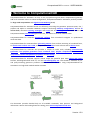
1 Welcome to ComputationalCAD
ComputationalCAD for AutoCAD is an easy to use, top-performing and robust computational geometry
add-on for AutoCAD. Due to its advanced algorithms, ComputationalCAD for AutoCAD is perfectly suitable
for large scale computations and Digital Terrain Modeling (DTM).
ComputationalCAD for AutoCAD focuses on efficiently processing the geometric primitives point, line /
polyline and 3dface in AutoCAD. Methods comprise conforming Delaunay triangulations, 2d and 3d
convex hulls, minimum enclosing rectangles and circles and 3d bounding boxes. In combination with
ComputationalCADs point-on-solid generation tool, this allows to container load 3d solids.
ComputationalCAD for AutoCAD reconstructs surfaces from unordered triangular or quadrilateral
wireframe data.
ComputationalCAD for AutoCAD allows generating meshes from surfaces consisting of unordered faces,
to convert such surfaces into a solid, to compute the silhouette of such surfaces and to colorize them.
ComputationalCAD for AutoCAD also provides a couple of useful tools, including point-on-entity
generation, fast polyline generation from unordered lines, polyline simplification, contour line
computation, surface interpolation / projection and face slicing.
ComputationalCAD for AutoCAD supports several simple but powerful plain ASCII import and export
formats, including Microsoft Excel csv, xml and stereolithography STL. This enables a workflow of preand post-processing geometric primitives outside AutoCAD and then using ComputationalCAD for
AutoCAD to run high-level methods within AutoCAD.
This document provides detailed help on all available commands, best practices and background
information. We are also looking forward to seeing you at www.computational-cad.com.
4
Version 1.5.0
ComputationalCAD for AutoCAD – USER MANUAL
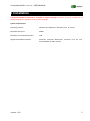
2 Installation
ComputationalCAD for AutoCAD is available in English language. However, it can be installed on all
supported products regardless of the product language.
System requirements:
Operating systems:
Windows XP, Windows 7, Windows Vista, 32 / 64 bit.
Minimum disk space:
50MB
Minimum recommended memory:
1GB
Supported Autodesk products:
AutoCAD, AutoCAD Mechanical, AutoCAD Civil 3D and
AutoCAD MAP 3D 2007 to 2012.
Version 1.5.0
5
ComputationalCAD for AutoCAD – USER MANUAL
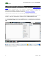
2.1 Install ComputationalCAD for AutoCAD
ComputationalCAD for AutoCAD will be installed for the current user and for all supported Autodesk
products that are currently installed on your computer. To install ComputationalCAD, double-click
computationalcad_setup.msi and follow the instructions. After the installation is complete, both
command line commands and menues will be available in all supported Autodesk products.
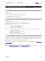
If the main menu is not visible in the current workspace, type ‘MENUBAR’ and set its value to 1.
If the toolbar is not visible, go to Tools  Toolbars  COMPUTATIONALCAD  ComputationalCAD (2010
or higher) or right-click in a docking region and directly select the COMPUTATIONALCAD toolbar.
You can manually load the customization file by typing “cuiload”. You can browse the customization file
(.cui for AutoCAD 2007-2009 or .cuix for AutoCAD 2010 and higher) in the ComputationalCAD installation
folder.
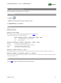
Figure 1: ComputationalCAD main menu
Figure 2: ComputationalCAD toolbar
6
Version 1.5.0
ComputationalCAD for AutoCAD – USER MANUAL
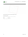
2.2 Uninstall ComputationalCAD for AutoCAD
Standard procedure
1. To uninstall ComputationalCAD for AutoCAD, you should first unload its customization file for
each installed Autodesk product. The easiest way to do this is by typing ‘CC:MENU:DELETE’ in the
command line.
2. Double-click on the file computationalcad_setup.msi and select the uninstall option.
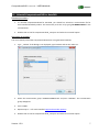
Alternative proceedure
You can manually unload the ComputationalCAD menu using AutoCAD methods.
1. Type ‘_cuiload’. If the dialog is not displayed, type ‘FILEDIA’ and set the value to 1.
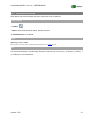
Figure 3: Unload customization file
2. Select the customization group ‘COMPUTATIONALCAD’ and press ‘UNLOAD’. The customization
group disappears.
3. Press ‘CLOSE’.
4. Repeat steps 1 – 3 for each installed supported Autodesk product.
5. Double-click on the file computationalcad_setup.msi and select the uninstall option.
Version 1.5.0
7
ComputationalCAD for AutoCAD – USER MANUAL
3 Import and export
ComputationalCAD for AutoCAD supports a couple of file formats that make it easy for standard users as
well as for developers to import data into AutoCAD and to export results for further post-processing.
The ASCII xyz and 3df formats allow to import and export point and 3dface data, respectively. Entity
coordinates are separated by comma, semicolon or blank separators and can be imported and exported
e.g. into Microsoft Excel as .csv format files.
The XML format is an easy to implement format for developers and may be a simple alternative to the
more complex dxfTM format. It allows to import and export point, line, polyline and 3dface entities with
layer and color information. Developer can download a .NET class to read and write this format at
www.computational-cad.com.
If the FILEDIA system variable is set to 1, dialogs are displayed. If the FILEDIA system variable is set
to 0, dialog boxes are not displayed. You can still request a file dialog box to appear by entering a
tilde (~) in response to the command's prompt.
8
Version 1.5.0
ComputationalCAD for AutoCAD – USER MANUAL
3.1 The XYZ point format
Provides ASCII import and export of point entities.
Input format
Arbitrary comment lines start with the character 'C', all other lines are split at the specified delimiter.
Empty lines are not feasible.
The first two terms (corresponding to the x and y coordinates, respectively) must be numerical. If a line
only contains two (numerical) terms, the z-coordinate is set to zero. An optional third term must be
numerical (the z-coordinate). Arbitrary comments can be placed after the third occurrence of the
delimiter in a line. Coordinates refer to UCS.
C Most simple format: x and y with only one delimiter. z is set to zero.
1.000, 2.000
C Also possible: x and y with two delimiters, z is set to zero
1.000, 2.000,
C x, y and z using two delimiters. Comment not possible!
1.000, 2.000, 3.000
C x, y and z, plus comment
1.000, 2.000, 3.000, Comment goes here...
Example output
The first line of the file is a comment line containing the file name and file generation date. All other lines
contain the x, y and z coordinates columnwise with the specified number of decimal digits (i.e. the
number of decimal digits after the decimal separator) and column width. The columns are separated by
the specified delimiter. Coordinates refer to UCS.
If the length of a formatted coordinate is greater than the specified column width, the respective cell is
filled with the character '*'. A warning message is displayed. In this case, increase the column width or
decrease the number of decimals.
Line four contains a y-coordinate greater than 9999.9999 or less than -999.9999, respectively.
C c:\test.pt generated
1.2345; -1.2345;
9999.9999;-999.9999;
1000.0000;*********;
Version 1.5.0
10.02.2010 15:16:10
0.0000;
0.0000;
0.0000;
9
ComputationalCAD for AutoCAD – USER MANUAL
3.1.1 Import from a xyz format file
Read UCS point coordinate data from an ASCII file.
Access methods
 Toolbar:
 Menu: ComputationalCAD  Import  Import points
 Command entry: CC:IO:XYZIN
Dialog
Specify file name:
Enter a valid file name with full path. A dialog is displayed depending on the FILEDIA settings.
Note
The coordinate delimiter is automatically detected. It must be one of comma (','), semicolon (';'), blank (' ')
or a tabulator or the method fails.
10
Version 1.5.0
ComputationalCAD for AutoCAD – USER MANUAL
3.1.2 Export to an xyz format file
Write UCS point coordinate data to an ASCII file.
Access methods
 Toolbar:
 Menu: ComputationalCAD  Export  Export points
 Command entry: CC:IO:XYZOUT
Dialog
Select points:
Select the points to export.
Specify file name:
Enter a valid file name with full path. A dialog is displayed depending on the FILEDIA settings.
If the specified file already exists, the following dialog occurs:
File already exists. Overwrite? [Yes, No]:
<Yes>:
The existing file will be irreversibly overwritten.
<No>:
Loops back (default)
Specify delimiter [Comma, Semicolon, Blank, Tab]:
<Comma>:
The coordinates will be separated by comma (',')
<Semicolon>:
The coordinates will be separated by semicolon (';') (default)
<Blank>:
The coordinates will be separated by blank (' ')
<Tab>:
The coordinates will be separated by a tabulator
Specify column width or [Fit]:
Enter the width of the column for each coordinate or 'F' for optimal width. Expects an integer value between 1 and 256 or 'F'. Default is <9>.
Specify number of decimal digits or [Float]:
Enter the number of decimal digits after the decimal separator of each coordinate or 'F' for maximum precision. Expects an integer value between
1 and 16 or ' F'. Default is <4>.
Note
Use the XML format to provide layer and color information.
Version 1.5.0
11
ComputationalCAD for AutoCAD – USER MANUAL
3.2 The 3d face format
Provides ASCII import and export of 3dface entities with layer information.
Input format
Arbitrary comment lines start with the character 'C', all other lines are split at the specified delimiter.
Empty lines are not feasible.
The first term must be the valid AutoCAD layer name of the 3d face. The UCS x, y and z coordinates of
each vertex follow. Note that an AutoCAD 3dface entity has always four vertices. To describe a triangular
face, the third and fourth vertex must be identical.
C Arbitrary comments
C Format: Layername,
tri, 1.0, 2.0, 3.0,
quad, 1.0, 2.0, 3.0,
go after ‘C’
x1, y1, z1, x2, y2, z2, x3, y3, z3, x4, y4, z4
4.0, 5.0, 6.0, 7.0, 8.0, 9.0, 7.0, 8.0, 9.0,
4.0, 5.0, 6.0, 7.0, 8.0, 9.0,10.0,11.0,12.0,
Example output
The first line of the file is a comment line containing the file name and file generation date. The second
line is a comment line containing format information. All other lines are data lines containing the x, y and
z coordinates of all four vertices columnwise using the specified number of decimal digits (i.e. the number
of decimal digits after the decimal separator) and column width. The columns are separated by the
specified delimiter. Coordinates refer to UCS.
If the length of a formatted coordinate is greater than the specified column width, the respective cell is
filled with the character '*'. A warning message is displayed. In this case, increase the column width or
decrease the number of decimals.
C c:\tmp\faces.3df generated 01.09.2010 13:55:59
C Format: Layername, x1, y1, z1, x2, y2, z2, x3, y3, z3, x4, y4, z4
tri, 1.0, 2.0, 3.0, 4.0, 5.0, 6.0, 7.0, 8.0, 9.0, 7.0, 8.0, 9.0,
quad, 1.0, 2.0, 3.0, 4.0, 5.0, 6.0, 7.0, 8.0, 9.0,10.0,11.0,12.0,
12
Version 1.5.0
ComputationalCAD for AutoCAD – USER MANUAL
3.2.1 Import a 3d face format file
Read 3dface UCS coordinate data with layer information from an ASCII file.
Access methods
 Toolbar:
 Menu: ComputationalCAD  Import  Import 3d faces
 Command entry: CC:IO:3DFIN
Dialog
Specify file name:
Enter a valid file name with full path. A dialog is displayed depending on the FILEDIA settings.
.
Note
The coordinate delimiter is automatically detected. It must be one of comma (','), semicolon (';'), blank (' ')
or a tabulator or the method fails.
Version 1.5.0
13
ComputationalCAD for AutoCAD – USER MANUAL
3.2.2 Export to a 3d face format file
Write 3dface UCS coordinate data with layer information to an ASCII file.
Access methods
 Toolbar:
 Menu: ComputationalCAD  Export  Export 3d faces
 Command entry: CC:IO:3DFOUT
Dialog
Select faces:
Select the 3d faces to write in the file.
Specify file name:
Enter a valid file name with full path. A dialog is displayed depending on the FILEDIA settings.
.
If the specified file already exists, the following dialog occurs:
File already exists. Overwrite? [Yes, No]:
<Yes>:
The existing file will be irreversibly overwritten.
<No>:
Loops back (default)
Specify delimiter [Comma, Semicolon, Blank, Tab]:
<Comma>:
The coordinates will be separated by comma (',')
<Semicolon>:
The coordinates will be separated by semicolon (';') (default)
<Blank>:
The coordinates will be separated by blank (' ')
<Tab>:
The coordinates will be separated by a tabulator
Specify column width or [Fit]:
Enter the width of the column for each coordinate or ‘F’ for optimal fit. Expects an integer value between 1 and 256 or ‘F’. Default is <9>.
Specify number of decimal digits or [Float]:
Enter the number of decimal digits after the decimal separator of each coordinate or ‘F’ for floating point precision. Expects an integer value
between 1 and 16 or ‘F’. Default is <4>.
Note
Use the XML format to provide layer and color information.
14
Version 1.5.0
ComputationalCAD for AutoCAD – USER MANUAL
3.3 The XML format
The XML format supports point, line, polyline and 3dface entities, each with color index and layer name.
Developer can download a .NET class with XML serializer / deserializer for this format at
www.computational-cad.com.
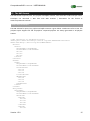
Example input and output
The XML scheme for point, line, polyline and 3dface entities is given below. Coordinates refer to UCS. The
polyline export supports 2d and 3d polylines. Imported polylines are always generated as 3d polyline
entities.
<?xml version="1.0" encoding="utf-8"?>
<EntityList xmlns:xsi="http://www.w3.org/2001/XMLSchema-instance"
xmlns:xsd="http://www.w3.org/2001/XMLSchema">
<Points>
<Point>
<LayerName></LayerName>
<ColorIndex></ColorIndex>
<X></X>
<Y></Y>
<Z></Z>
</Point>
</Points>
<Lines>
<Line>
<LayerName></LayerName>
<ColorIndex></ColorIndex>
<StartVertex>
<X></X>
<Y></Y>
<Z></Z>
</StartVertex>
<EndVertex>
<X></X>
<Y></Y>
<Z></Z>
</EndVertex>
</Line>
</Lines>
<Polylines>
<PolyLine>
<LayerName></LayerName>
<ColorIndex></ColorIndex>
<Vertices>
<Vertex>
<X></X>
<Y></Y>
<Z></Z>
</Vertex>
<Vertex>
<X></X>
Version 1.5.0
15
ComputationalCAD for AutoCAD – USER MANUAL
<Y></Y>
<Z></Z>
</Vertex>
<Vertex>
<X></X>
<Y></Y>
<Z></Z>
</Vertex>
</Vertices>
</PolyLine>
</Polylines>
<Faces>
<Face>
<LayerName></LayerName>
<ColorIndex></ColorIndex>
<Vertex1>
<X></X>
<Y></Y>
<Z></Z>
</Vertex1>
<Vertex2>
<X></X>
<Y></Y>
<Z></Z>
</Vertex2>
<Vertex3>
<X></X>
<Y></Y>
<Z></Z>
</Vertex3>
<Vertex4>
<X></X>
<Y></Y>
<Z></Z>
</Vertex4>
</Face>
</Faces>
</EntityList>
16
Version 1.5.0
ComputationalCAD for AutoCAD – USER MANUAL
3.3.1 Import a XML entity format file
Read UCS point, line, polyline and 3dface data with layer and color information from an XML file.
Access methods
 Toolbar:
 Menu: ComputationalCAD  Import  Import xml
 Command entry: CC:IO:XMLIN
Dialog
Specify file name:
Enter a valid file name with full path. A dialog is displayed depending on the FILEDIA settings.
.
Note
Polylines will be inserted as 3d polyline entities.
Version 1.5.0
17
ComputationalCAD for AutoCAD – USER MANUAL
3.3.2 Export to a XML entity format file
Write UCS point, line, polyline and 3dface data with layer and color information to an XML file.
Access methods
 Toolbar:
 Menu: ComputationalCAD  Export  Export xml
 Command entry: CC:IO:XMLOUT
Dialog
Select objects:
Select the point, line, polyline and 3d face objects to write to the file.
Specify file name:
Enter a valid file name with full path. A dialog is displayed depending on the FILEDIA settings.
.
If the specified file already exists, the following dialog occurs:
File already exists. Overwrite? [Yes, No]:
<Yes>:
The existing file will be irreversibly overwritten.
<No>:
Loops back (default)
Note
Polylines can be 2d or 3d polylines. However, polylines will always be imported as 3d polyline entities.
18
Version 1.5.0
ComputationalCAD for AutoCAD – USER MANUAL
3.4 The STL format
Provides import and export of ASCII and binary STL files.
Format
STL is a file format native to the stereolithography CAD software created by 3D Systems. This file format is
it is widely used for rapid prototyping and computer-aided manufacturing. STL files describe only the
surface geometry of a three dimensional object without any representation of color, texture or other
common CAD model attributes. The STL format specifies both ASCII and binary representations. Binary
files are more common, since they are more compact. Both formats are non-proprietary and can be
studied in detail e.g. at http://en.wikipedia.org/wiki/STL_(file_format).
Version 1.5.0
19
ComputationalCAD for AutoCAD – USER MANUAL
3.4.1 Import a STL format file
Read 3dfaces defined in an ASCII or binary format STL file.
Access methods
 Toolbar:
 Menu: ComputationalCAD  Import  Import STL
 Command entry: CC:IO:STLIN
Dialog for ASCII format
Insert on layer [Current/specify Name/by STL] <by STL>:
Specify the layer the faces will be inserted.
<Current>:
The points will lie on the current layer.
<by STL>:
The points will lie on a layer named by the solid name in the ASCII STL file header. If the layer does not exist, it will be
created. (Default)
<specify Name>:
The following dialog is displayed:
Specify layer name:
Enter the name of the layer the points shall be added to. If the layer does not exist, it will be generated.
Dialog for binary format
Insert on layer [Current/specify Name] <Current>:
Specify the layer the faces will be inserted.
<Current>:
The points will lie on the current layer. (Default)
<specify Name>:
The following dialog is displayed:
Specify layer name:
Enter the name of the layer the points shall be added to. If the layer does not exist, it will be generated.
Note
ASCII or binary format STL will be detected automatically.
Some elder STL formats may only accept positive coordinates. ComputationalCAD for AutoCAD accepts
both positive and negative XYZ coordinates. However, you will be warned if negative coordinates have
been detected during read.
In both ASCII and binary versions of STL, the facet normal should be a unit vector pointing outwards from
the solid object (“right hand rule”). ComputationalCAD for AutoCAD ignores facet normal vectors.
However, you will be warned if inconsistent facet normals have been detected.
In binary STL, ComputationalCAD for AutoCAD accepts color information in VisCAM / SolidView format
(RGB information in the attribute byte count, see http://en.wikipedia.org/wiki/STL_(file_format) ).
20
Version 1.5.0
ComputationalCAD for AutoCAD – USER MANUAL
Coordinates always refer to the WCS.
Example ASCII STL format command line output
STL solid name
:
Number of triangles read
:
Number of degenerate triangles:
Has negative coordinates
:
Inconsistent facet normals
:
Solid inserted on layer surface
surface
126523
0
False
True
Example binary STL format command line output
Number of triangles read
:
Number of degenerate triangles:
Has negative coordinates
:
Inconsistent facet normals
:
File contains colors
:
Version 1.5.0
126523
0
False
True
True
21
ComputationalCAD for AutoCAD – USER MANUAL
3.4.2 Export a STL format file
Writes 3dfaces in an ASCII or binary format STL file.
Access methods
 Toolbar:
 Menu: ComputationalCAD  Export  Export to STL
 Command entry: CC:IO:STLOUT
Dialog for ASCII format
Specify STL type [Binary/Ascii] <Binary>:
Specify the STL format type.
<Binary>: Output format will be STL binary. (Default)
<ASCII >: Output format will be STL ASCII.
Specify STL solid name <0>:
Specify the name of the solid. Default is the layer name of the first selected face.
Dialog for binary format
Specify STL type [Binary/Ascii] <Binary>:
Specify the STL format type.
<Binary>:
Output format will be STL binary. (Default)
<ASCII >:
Output format will be STL ASCII.
Note
Some elder STL formats may only accept positive coordinates. ComputationalCAD for AutoCAD accepts
both positive and negative XYZ coordinates to write. However, you will be warned if negative coordinates
have been detected during write.
ComputationalCAD for AutoCAD, the facet normal is always a unit vector pointing outwards from the solid
object (“right hand rule”). ComputationalCAD for AutoCAD cant not write degenerate faces (i.e faces with
collinear or identical vertices where a face normal can not be computed). You will be warned if
inconsistent facet normals have been detected.
In binaly format STL, ComputationalCAD for AutoCAD automatically writes color information in VisCAM /
SolidView
format
(RGB
information
in
the
attribute
byte
count,
see
http://en.wikipedia.org/wiki/STL_(file_format) ).
Coordinates always refer to the WCS.
22
Version 1.5.0
ComputationalCAD for AutoCAD – USER MANUAL
Example command line output
Number of triangles written
: 126401
Number of degenerate triangles: 0
Has negative coordinates
: False
STL file in binary format written to
C:\Users\Christian\Documents\entities_col.stl
Version 1.5.0
23
ComputationalCAD for AutoCAD – USER MANUAL
4 Handling point primitives
ComputationalCAD for AutoCAD provides a couple of methods to generate and modify point data to
generate input for other methods. Available methods allow to

reengineer point data from a surface consisting of 3dface entities,

generate point data from text entities,

reduce the amount of point data,

generate point data by subdivision of spline, line, polyline, circle or arc entities,

eliminate duplicate points with identical xy-coordinates in UCS within a specified range,

blur the xy-coordinates of points in UCS,

project points onto a surface consisting of 3dface entities.
Influence the appearance of points by setting the AutoCAD _ddptype value.
24
Version 1.5.0
ComputationalCAD for AutoCAD – USER MANUAL
4.1 Generate points on primitives
Generate equidistant points on various AutoCAD primitives.
Access methods
 Toolbar:
 Menu: ComputationalCAD  Generate points on primitives
 Command entry: CC:POINTS:GENERATE
Dialog
Select entity type <Lines, Texts, Circles, Ellipses, Arcs, Splines,
3dFaces, Polylines, ALL>:
<Lines>:
Generates equidistant points on lines.
<Texts>:
Reads the text property of a single line text and generates a point at the insertion point of the text
if the text is numerical.
<Circles>:
Generates equidistant points on the perimeter of circles.
<Ellipses>:
Generates equidistant points on the perimeter of ellipses.
<Arcs>:
Generates equidistant points on the perimeter of arcs.
<Splines>:
Generates equidistant points on splines.
<3dFaces>:
Generates points at the vertices of 3d faces.
<Polylines>:
Generates equidistant points on linear 2d and 3d polylines.
<ALL>:
Generates points on all available entities. (default)
For all entity types except <Texts> and <3dFace>, the following dialog will be displayed:
Enter maximum subdivision distance or 0 for no subdivision:
Enter the maximum distance between two equidistant points generated on the specified entities. Expects a value greater than 0. Default is <1>.
Insert on layer [Current/specify Name] :
<Current>:
The points will lie on the current layer. (Default)
<specify Name>:
The following dialog is displayed:
Specify layer name:
Enter the name of the layer the points shall be added to. If the layer does not exist, it will be generated.
Insert as block? <Yes, No> :
<Yes>:
The following dialog is displayed:
Specify block name:
Enter the name of the block the points shall be added to. If the block does not exist, it will be generated.
<No>:
The points will be inserted in the model space. (Default)
Summary
On each entity, equidistant points are generated so that the distance between two points is not greater
than the specified subdivision distance. Duplicate points will be eliminated. A zero subdivision distance
does not affect <Texts> and <3dFaces> entities. For all other entities, it has the following effect:
Version 1.5.0
25
ComputationalCAD for AutoCAD – USER MANUAL
<Lines> and <Splines>: points are generates at start and end points only.
<Circles>, <Ellipses> and <Arcs>: points are generated at the center points only.
<Polylines>: points are generates at each vertex of a polyline.
Example
Figure 4: 107k 3dface entities
Figure 5: 54k corner vertices of above faces generated using the Generate points command
26
Version 1.5.0
ComputationalCAD for AutoCAD – USER MANUAL
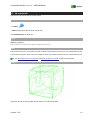
4.2 Generate points on solids
Generate points on AutoCAD Solid3D entities. This method is only available for AutoCAD versions 2010
or higher.
Access methods
 Toolbar:
 Menu: ComputationalCAD  Generate points on solids
 Command entry: CC:SOLIDS:TESSELATE
Dialog
Select 3d solids:
Select one or more Solid3d entities.
Specify maximum node spacing:
Enter the maximum distance between two points generated on the solid(s). Expects a value greater than 0. Default is 1/100 of the maximum
diagonal of the geometric extends of all selected solids.
Insert on layer [Current/specify Name] :
<Current>:
The points will lie on the current layer. (Default)
<specify Name>:
The following dialog is displayed:
Specify layer name:
Enter the name of the layer the points shall be added to. If the layer does not exist, it will be generated.
Insert as block? <Yes, No> :
<Yes>:
The following dialog is displayed:
Specify block name:
Enter the name of the block the points shall be added to. If the block does not exist, it will be generated.
<No>:
The points will be inserted in the model space. (default)
Summary
The solid may be arbitrary complex. The generated points are the corner vertices of the tessellation of the
solid. Due to AutoCAD internals, the actual distance between two points on a solid may be significantly
smaller than the maximum node spacing.
Version 1.5.0
27
ComputationalCAD for AutoCAD – USER MANUAL
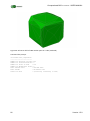
Example
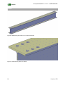
Figure 6: 9008 points generated on an I-beam with holes
Figure 7: Detail view of points on I-beam
28
Version 1.5.0
ComputationalCAD for AutoCAD – USER MANUAL
4.3 Eliminate duplicate points in UCS xy plane
Eliminate duplicate points with identical x and y coordinates in UCS.
Access methods
 Toolbar:
 Menu: ComputationalCAD  Eliminate 2d identical points
 Command entry: CC:POINTS:ELIM2D
Dialog
Select points:
Select the points to eliminate duplicates from.
Specify snap radius:
Enter the snap radius. Expects a value greater or equal 0. Default is <0>.
Point to keep [Highest/Lowest]:
<Highest>:
The point with the highest z-coordinate within the snap radius is kept. (default)
<Lowest>:
The point with the lowest z-coordinate within the snap radius is kept.
Summary
If the UCS z-coordinate of point p1 is greater than the z-coordinate of point p2, p2 will be eliminated if
<Highest> was specified. Otherwise, p1 will be eliminated. If the UCS z-coordinates of both points are
identical, any of the points will be eliminated. All coordinates refer to UCS.
Figure 8: Two points and respective snap circles
Use the native AutoCAD command overkill to eliminate identical 3d points.
Version 1.5.0
29
ComputationalCAD for AutoCAD – USER MANUAL
Example
Figure 9: 54k vertices reduced to 28k vertices using the Elim2d command
30
Version 1.5.0
ComputationalCAD for AutoCAD – USER MANUAL
4.4 Blur points in UCS xy plane
Blur the x and y coordinates of a point in UCS.
Access methods
 Toolbar:
 Menu: ComputationalCAD  Blur points
 Command entry: CC:POINTS:BLUR
Dialog
Select points:
Select the points to blur.
Specify blur radius:
Enter the blur radius. Expects a value greater than 0. Default is 1e-9.
Summary
This command randomly offsets the UCS x and y coordinates within the specified blur radius. Blurring
rastered point data creates biunique data for a triangulation.
Example
Figure 10: 85 points on an equidistant raster (black) and blurred points (blue)
Version 1.5.0
31
ComputationalCAD for AutoCAD – USER MANUAL
4.5 Project points onto a surface
Project points onto a surface consisting of 3dface entities.
Access methods
 Toolbar:
 Menu: ComputationalCAD  Project points
 Command entry: CC:POINTS:PROJECT
Dialog
Select faces:
Select the 3dfaces defining the surface
Select points:
Select the points to project.
Specify projection direction [X/Y/Z/Ucs/2Points]:
Select the projection direction.
<X>:
The points are projected in global X-direction
<Y>:
The points are projected in global Y-direction.
<Z>:
The points are projected in global Z-direction. (default)
<Ucs>:
The points are projected in UCS z-direction.
<2Points>:
The points are projected in a user defined projection direction. The following dialog occurs:
Specify first point
Select the first point of the projection direction.
Specify second point
Select the second point of the projection direction.
Insert on layer [Current/by Face/by Point]:
Select the layer assignment for the projected points.
<Current>:
The projected points will be inserted on the current layer.
<by Face>:
The projected points will be inserted on the layer of the 3dface the point was projected onto. (default)
<by Point>:
The projected points will be inserted on the layer of the original point.
Delete original points [Yes/No]:
Specify if the original points shall be deleted.
<Yes>:
The original points will be erased.
<No>:
The original points will not be erased. (default)
Point to keep [Highest/Lowest]:
<Highest>:
The point with the highest z-coordinate is kept. (default)
<Lowest>:
The point with the lowest z-coordinate is kept.
32
Version 1.5.0
ComputationalCAD for AutoCAD – USER MANUAL
Example
Figure 11: 54k vertices (black) projected onto a surface consisting of 104k faces (not shown for clarity)
Version 1.5.0
33
ComputationalCAD for AutoCAD – USER MANUAL
5 Handling line primitives
ComputationalCAD for AutoCAD provides several methods to process line entities. Available methods
allow to
34

generate polylines from unordered lines

simplify polylines by reducing the number of vertices

slice multiple lines on a 3d slicing plane

project lines onto a surface consisting of 3dface entities.
Version 1.5.0
ComputationalCAD for AutoCAD – USER MANUAL
5.1 Generate polylines from a set of unordered lines
Generate 3d polylines from a set of unordered lines.
Access methods
 Toolbar:
 Menu: ComputationalCAD  Convert lines to polylines
 Command entry: CC:LINES:TOPLINE
Dialog
Select lines:
Select the lines to convert into 3d polylines
Specify number of relevant decimal digits:
Specify the number of relevant decimal digits after the decimal separator. All coordinates will be rounded to the specified value. Expects an
integer value between 0 and 12. Default is <8>.
Eliminate zero length segments [Yes/No]:
With r being the number of relevant decimal digits, specify if segments with a length smaller then
10
r
<Yes>:
Polyline segments shorter than
<No>:
The polyline will contain all segments.
10 r
shall be eliminated.
will be eliminated. (default)
Delete original lines [Yes/No]:
Specify if the original lines shall be deleted.
<Yes>:
The original lines will be deleted.
<No>:
The original lines will not be deleted. (default)
Summary
The command converts all selected lines into POLY3D entities and joins adjoining lines if
1. the lines lie on the same layer
2. the lines have the same color
3. the lines have a common start or endpoint, respectively, within the precision specified.
The number of relevant decimal digits specifies how many decimal digits after the decimal separator have
to be identical in order to consider start or end vertex, respectively, of two adjoining line segments to be
identical. The coordinates of all vertices will be rounded to the specified value.
Branching is not feasible for AutoCAD polyline objects. The layer and color properties of incident lines are
used to decide which lines to connect at a branching point. However, if multiple options exist, the result
will be arbitrary.
Version 1.5.0
35
ComputationalCAD for AutoCAD – USER MANUAL
Example
Figure 12: Four 3d polylines (one highlighted), generated from 10 line segments. Since all lines have the
same layer and color properties, the behavior at the branching points is arbitrary.
Command line prompt:
Number of segments added
Number of zero-length segments
Number of polylines generated
: 10
: 0
: 4
Figure 13: 201 polylines (one selected), generated at once from 35330 individual (contour) line segments
Command line prompt:
Number of segments added
Number of zero-length segments
Number of polylines generated
36
: 35330
: 0
: 201
Version 1.5.0
ComputationalCAD for AutoCAD – USER MANUAL
5.2 Simplify polylines
Reduce the number of AutoCAD 3d polyline vertices so that the maximum spatial distance between any
points on the original polyline to the simplified polyline is smaller than specified.
Access methods
 Toolbar:
 Menu: ComputationalCAD  Simplify polylines
 Command entry: CC:LINES:SIMPLIFYPLINE
Dialog
Select polylines:
Select the polylines to simplify. This may be 2d or 3d polylines.
Specify epsilon range:
Specify the maximum spatial distance between any point on the original polyline to the simplified polyline. Expects a positive value or zero.
Keep original polylines [Yes/No]:
Specify if the original polylines shall be deleted.
<Yes>:
The original lines will not be deleted. (default)
<No>:
The original lines will be deleted.
Summary
The command creates a new 3d polyline sharing start and end vertex with the original polyline.
Successively going through the intermediate vertices of the original polyline, an intermediate vertex will
only be added to the simplified polyline if necessary to ensure that the maximum spatial distance
between any points on the original polyline to the simplified polyline is smaller than specified.
Version 1.5.0
37
ComputationalCAD for AutoCAD – USER MANUAL
Example
Figure 14:203 vertices in one polyline (black) reduced to 23 vertices in a simplified polyline (red)
Command line prompt:
Number
Number
Number
Number
of
of
of
of
vertices before
:
vertices after
:
polylines processed:
polylines failed
:
203
23
1
0
Figure 15: A polyline with 1682 vertices (left) reduced to a polyline with 182 vertices (right)
Command line prompt:
Number
Number
Number
Number
38
of
of
of
of
vertices before
:
vertices after
:
polylines processed:
polylines failed
:
1682
182
1
0
Version 1.5.0
ComputationalCAD for AutoCAD – USER MANUAL
Figure 16: 37832 vertices in 307 polylines (one selected) reduced to 5851 vertices
Command line prompt:
Number
Number
Number
Number
of
of
of
of
vertices before
:
vertices after
:
polylines processed:
polylines failed
:
Version 1.5.0
37832
5851
307
0
39
ComputationalCAD for AutoCAD – USER MANUAL
5.3 Slice lines
Slice 3d line entities.
Access methods
 Toolbar:
 Menu: ComputationalCAD  Slice lines
 Command entry: CC:LINES:SLICE
Dialog
Select lines:
Select the lines to slice.
Specify origin point of plane:
Specify the origin point of the slicing plane.
Specify point on positive x-axis:
Specify a point on the x-axis of the slicing plane.
Specify third point on plane:
Specify a third point on the slicing plane.
Specify point on side to keep or [keep Both sides]:
Specify a point on the side to keep or enter ‘B’ to keep both sides. Default is <B>
Summary
The command slices an arbitrary number of 3d line entities on a 3d slicing plane.
Example
Figure 17: A couple of lines sliced along a vertical slicing plane (red)
40
Version 1.5.0
ComputationalCAD for AutoCAD – USER MANUAL
5.4 Project lines onto a surface
Project lines onto a surface consisting of 3dface entities.
Access methods
 Toolbar:
 Menu: ComputationalCAD  Project lines
 Command entry: CC:LINES:PROJECT
Dialog
Select faces:
Select the 3dfaces defining the surface
Select lines:
Select the lines to project.
Specify projection direction [X/Y/Z/Ucs/2Points]:
Select the projection direction.
<X>:
The lines are projected in global X-direction
<Y>:
The lines are projected in global Y-direction.
<Z>:
The lines are projected in global Z-direction. (default)
<Ucs>:
The lines are projected in UCS z-direction.
<2Points>:
The lines are projected in a user defined projection direction. The following dialog occurs:
Specify first point
Select the first point of the projection direction.
Specify second point
Select the second point of the projection direction.
Insert on layer [Current/by Face/by Line]:
Select the layer assignment for the projected lines.
<Current>:
The projected lines will be inserted on the current layer. The colour of each line will be the colour of its 3dface.
<by Face>:
The projected line will be inserted on the layer of the 3dface the line was projected onto. (default)
<by Line>:
The projected lines will be inserted on the layer of the original lines.
Delete original lines [Yes/No]:
Specify if the original lines shall be deleted.
<Yes>:
The original lines will be erased.
<No>:
The original lines will not be erased. (default)
Summary
The lines will be projected onto faces lying above and below the line in projection direction. For each line,
start and end point are projected onto the surface. If a line crosses an edge of a face in projection
direction, it will be split at the projected intersection point of edge and line. Consequently, there will be
more projected lines than original lines in a general case.
Version 1.5.0
41
ComputationalCAD for AutoCAD – USER MANUAL
The projection onto a specific face fails if the normal vector of the face is perpendicular to the projection
vector or if the line to be projected runs parallel to the projection direction.
If the lines are inserted in the current layer, the colour of each line will be the colour of the face it is
projected onto.
Example
Figure 18: Four lines in the xy plane and their projection onto a surface
Command line prompt:
Number of lines projected
: 850
Number of failed faces
: 0
Faces parallel to projection direction: 0
Lines parallel to projection direction: 0
42
Version 1.5.0
ComputationalCAD for AutoCAD – USER MANUAL
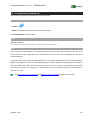
5.5 Develop a polyline
Compute the development (profile) in the xy plane of a 3d polyline.
Access methods
 Toolbar:
 Menu: ComputationalCAD  Develop polyline
 Command entry: CC:LINES:DEVELOP
Dialog
Select polyline:
Select a polyline, 2d polyline or 3d polyline consisting exclusively of line segments.
Reverse polyline [Yes/No]:
Specify if the development shall be computed for the reverse order of polyline vertices.
<Yes>:
Compute the development for the reverse order of polyline vertices.
<No>:
Compute the development for the normal order of polyline vertices. (default)
Specify range [Yes/No]:
Specify if you want to develop a specific arc length range of the polyline.
<No>:
Compute the development for entire polyline. (default)
<Yes>:
Compute the development for an arc length range of the polyline. The following dialog is displayed:
Specify start arc length
Specify the arc length of the polyline from where to start to compute the development. Default is 0.
Specify end arc length
Specify the arc length of the polyline where to stop to compute the development. Expects a positive double value. If greater
than the maximum length of the polyline, the development will be computed until the maximum length of the polyline.
Specify z-scaling <1>:
Specify a scaling for the z-heights of the polyline. Expects a positive double value. Default is 1.
Include first derivative (slope) [Yes/No]:
Specify if the first derivative (profile slope) shall be drawn too.
<Yes>:
The first derivative will be drawn together with the development.
<No>:
The first derivative will not be drawn. (default)
Specify outfile type [DWG/DXF]:
Specify if the output file type.
<DWG>:
The output file will be saved in the current dwg format.
<DXF>:
The original lines will be saved in the current dxf format. (default)
Depending on the FILEDIA setting, either a file dialog is displayed or the outfile name must be entered directly.
Version 1.5.0
43
ComputationalCAD for AutoCAD – USER MANUAL
Summary
The profile of a polyline is the development of the Z-height over the XY length of the polyline. The
command draws the XY projection of the polyline on the X-axis and the Z-height of the polyline on the Yaxis. The development is saved either in AutoCAD dwg or dxf format.
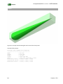
Example
Figure 19: A 3d polyline (red), its development (black) and the first derivative of the development (cyan)
Command line prompt:
Number of vertices :
Start arc length
:
End arc length
:
Delta arc length
:
Start ground length:
End ground length :
Delta ground length:
Minimum slope [%] :
at ground length:
Maximum slope [%] :
at ground length:
Minimum elevation :
Maximum elevation :
Delta elevation
:
44
701.0000
0.0000
9425.7085
9425.7085
0.0000
8736.6754
8736.6754
-201.0726
4468.3306
383.3087
4814.5793
5691.0948
6345.7523
654.6575
Version 1.5.0
ComputationalCAD for AutoCAD – USER MANUAL
6 Handling face primitives
ComputationalCAD for AutoCAD provides several methods to process 3dface entities. Available methods
allow to

compute contour lines of a surface consisting of 3dface entities

slice a surface consisting of 3dface entities
Version 1.5.0
45
ComputationalCAD for AutoCAD – USER MANUAL
6.1 Compute contour lines
Compute contour lines of a surface consisting of 3dface entities.
Access methods
 Toolbar:
 Menu: ComputationalCAD  Compute contour lines
 Command entry: CC:FACES:CONTOUR
Dialog
Select faces:
Select the 3dfaces defining the surface
Specify reference plane [Wcs/Ucs/3Point]:
Specify the plane to refer the elevation.
<Wcs>:
The elevation refers to the z-axis of the global coordinate system. (default)
<Ucs>:
The elevation refers to the z-axis of the UCS coordinate system.
<3Point>:
The elevation refers to the z-axis of a user defined coordinate system
Specify start elevation:
Enter the start elevation. The elevation refers to the z-axis of the reference plane specified above. Expects any numeric value. Default is <0>.
Specify end elevation:
Enter the start elevation. The elevation refers to the z-axis of the reference plane specified above. Expects any numeric value. Default is <0>.
Specify spacing:
Specify the spacing between two contour lines. The spacing refers to the z-axis of the reference plane specified above. Expects a positive, nonzero value. Default is <1>.
Insert on layer [Current/by Face/by Elevation/by Index]:
Specify on which layer the contour lines shall be inserted.
<Current>:
The contour lines will be inserted on the current layer.
<by Face>:
The contour lines will be inserted on the layer of the respective face.
<by Elevation>:
The contour lines will be inserted on a layer with the layer name containing the elevation of the contour line. The layer will be
created it if it does not exist. (default) Following dialog is displayed:
<by Index>:
The contour lines will be inserted on a layer with the layer name containing the index of the contour line, starting from 1.
The layer will be created it if it does not exist. Following dialog is displayed:
Specify prefix string
Specify the prefix of the layer name if <by Elevation> or <by Index> has been selected. Default is ‘Contour_line_’.
Summary
The contour lines will be inserted as AutoCAD 3d polyline entities. Regardless of the selected layer
insertion method, the color of a segment is always set to the color of the respective face. The contour
lines are computed in planes parallel to the specified reference plane.
46
Version 1.5.0
ComputationalCAD for AutoCAD – USER MANUAL
Example
Figure 20: App. 180k contour lines in 2045 polylines computed from app. 107k faces.
Command line prompt:
Failed intersections
:
Degenerate intersections :
Total number of segments :
Total number of polylines:
Version 1.5.0
0
0
180439
2045
47
ComputationalCAD for AutoCAD – USER MANUAL
6.2 Slice a surface
Slice a surface consisting of 3dface entities.
Access methods
 Toolbar:
 Menu: ComputationalCAD  Slice surface
 Command entry: CC:FACES:SLICE
Dialog
Select faces:
Select the 3dfaces defining the surface.
Specify origin point of plane:
Select the origin point of the slicing plane.
Specify point on positive x-axis:
Select a point on the positive x-axis of the slicing plane.
Specify third point on plane:
Select a third point on the slicing plane.
Specify point on side to keep or [keep Both sides]:
Select a point on the side of the slicing plane to keep or ‘B’ to keep both sides. Default is <B>.
Keep coplanar faces [Yes/No]:
Select if faces coplanar to the slicing plane shall be kept. Default is <Yes>.
Summary
The command slices a surface consisting of AutoCAD 3dface entities analogously to the AutoCAD slice
solid command. Faces that intersect the slicing plane will be erased and replaced by two or three faces
that respect the slicing plane. The orientation of the faces will be maintained.
48
Version 1.5.0
ComputationalCAD for AutoCAD – USER MANUAL
Example
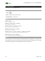
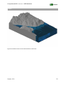
Figure 21: A sliced surface. Faces below slicing plane coloured blue, faces above slicing plane coloured
green
Command line prompt:
Failed faces
: 0
Faces sliced
: 2170
Faces remaining: 109647
Figure 22: Sliced surface – detail (top view)
Version 1.5.0
49
ComputationalCAD for AutoCAD – USER MANUAL
6.3 Convert unordered faces to mesh
Convert a surface consisting of unordered 3dface entities into a 3d mesh. This method is only available
for AutoCAD versions 2010 or higher.
Access methods
 Toolbar:
 Menu: ComputationalCAD  Convert faces to mesh
 Command entry: CC:FACES:TOMESH
Dialog
Select faces:
Select the 3dfaces defining the surface.
Delete original faces [Yes/No]:
Select if the original faces shall be deleted. Default is <Yes>.
Summary
A mesh is an advanced data structure that has several advantages over unordered faces:
1. The visualization performance for a mesh is several magnitudes better than for unordered faces.
A mesh easily allows orbiting millions of faces with full shading in real time.
2. Bitmap textures can be applied on a mesh in a whole allowing to produce high quality renderings
e.g. of landscapes.
3. A mesh can be smoothed.
4. A mesh is stored with app. 25% less disk space than unordered triangular faces.
A mesh can simply be exploded into its underlying faces again. The command combines unordered
AutoCAD 3d faces with identical layer and color properties to an AutoCAD mesh. Consequently, the
command creates as much meshes as there are faces with different layer and color properties.
50
Version 1.5.0
ComputationalCAD for AutoCAD – USER MANUAL
Example
Figure 23: Two meshes generated from 107k faces
Command line prompt:
Mesh
0:
Layer name
:
Number of vertices:
Number of faces
:
Mesh
1:
Layer name
:
Number of vertices:
Number of faces
:
Version 1.5.0
water
23605
45457
ground
32139
62255
51
ComputationalCAD for AutoCAD – USER MANUAL
6.4 Convert unordered faces to solid
Convert a surface consisting of unordered 3dface entities into a 3d solid by extrusion.
Access methods
 Toolbar:
 Menu: ComputationalCAD  Convert faces to solid
 Command entry: CC:FACES:TOSOLID
Dialog
Select faces:
Select the 3dfaces defining the surface.
Specify reference plane [Wcs/Ucs/3Point]:
Specify the extrusion reference plane. Default is <Wcs>.
Extrusion height in actual Z:
Specify the extrusion height with respect to the global z-axis. Default is <-1>.
Minimum projected edge length:
Specify the minimum length of the projection of the faces onto the reference plane. Default is <0.01>.
Union solids [Yes/No]:
Select if the extruded solids shall be united. Default is <Yes>.
Summary
This method extrudes each face in z-direction and unites the resulting solids. In order to do this, the
projection of the input faces onto the reference plane must not be degenerate. In order to achieve this,
the projected faces will be healed so that no projected edge will be shorter than specified.
Converting faces to solids allows for numerous advanced operations, including Boolean operations and
mass property computation. While extrusion is computationally not costive, AutoCAD solids are not
optimized for Boolean union operation performance of tens or hundreds of thousands of sub-entities.
Thus, being theoretically unbound in the number of input faces, this method does practically not support
extremely large input with the unite solids option. 5000 to 10000 faces may be united in about a minute.
52
Version 1.5.0
ComputationalCAD for AutoCAD – USER MANUAL
Example
Figure 24: Rendered view on two solids build from 107k faces
Version 1.5.0
53
ComputationalCAD for AutoCAD – USER MANUAL
6.5 Compute silhouette of unordered faces
Compute the silhouette region of a surface consisting of unordered 3dface entities on a reference plane.
Access methods
 Toolbar:
 Menu: ComputationalCAD  Compute silhouette
 Command entry: CC:FACES:SILHOUETTE
Dialog
Select faces:
Select the 3dfaces defining the surface.
Specify reference plane [Wcs/Ucs/3Point]:
Specify the reference plane of the silhouette. Default is <Wcs>.
Minimum projected edge length:
Specify the minimum length of the projection of the faces onto the reference plane. Default is <0.01>.
Summary
The silhouette of a surface is the visible outer bound of all faces. In order to do this, the projection of the
input faces onto the reference plane must not be degenerate. In order to achieve this, the projected faces
will be healed so that no projected edge will be shorter than specified.
54
Version 1.5.0
ComputationalCAD for AutoCAD – USER MANUAL
Example
Figure 25: 45k faces and silhouette region thereof (below)
Version 1.5.0
55
ComputationalCAD for AutoCAD – USER MANUAL
6.6 Colorize face properties
Colorize various properties of a surface consisting of 3d faces.
Access methods
 Toolbar:
 Menu: ComputationalCAD  Colorize faces
 Command entry: CC:FACES:COLORIZE
Dialog
Select faces:
Select the 3dfaces defining the surface.
Specify target property [ARea/Center Z/minimum ANgle/MINimumZ/MAXimumZ]
<ARea>:
Specify the property to colorize. Default is <ARea>.
Specify number of colors <6>:
Specify the number of colors to use Expects an integer between 2 and 32768. Default is <6>.
Specify lower cutoff percentage <0>:
Specify the the lower cutoff percentage. Default is <0>.
Specify upper cutoff percentage <100>:
Specify the the upper cutoff percentage. Default is <100>.
Note
The faces will be colorized in the order blue – cyan – green – yellow – red – magenta where the blue color
value is assigned to the face(s) with the smallest selected target property value and the magenta color
value is assigned to the face(s) with the highest selected target property value. The cutoff percentages
allow specifying the color of the minimum and maximum target property values as shown in the first
example.
The center Z, minimum Z and maximum Z target properties are best applicable to a terrain surface.
The minimum Angle property allows visualizing the triangulation quality.
The area property visualizes areas with high “density” of the faces defining a surface (densit plot).
56
Version 1.5.0
ComputationalCAD for AutoCAD – USER MANUAL
Example
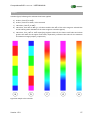
In below figure, following color schemes have been applied:
a) 6 colors, from 0% to 100%
b) 6 colors, from 0% to 100%, colors reversed
c) 100 colors, from 0% to 100%
d) 100 colors, from 20% to 80% (i.e. all values smaller than 20% of the value range are colored blue
and all values greater than 80% of the value range are colored magenta)
e) 100 colors, from -20% to 140%. Specifying negative values for the lower cutoff value and values
greater than 100% for the upper cutoff value, respectively, influences the colors for the minimum
and maximum target property, respectively.
Figure 26: Sample color schemes
Version 1.5.0
57
ComputationalCAD for AutoCAD – USER MANUAL
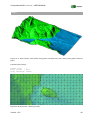
Figure 27: Top view on a terrain with colored minimum z-height property.
Figure 28: Perspective view on a terrain with colored minimum z-height property.
58
Version 1.5.0
ComputationalCAD for AutoCAD – USER MANUAL
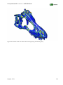
Figure 29: Dinosaur skull scan with colored area property (face density plot).
Version 1.5.0
59
ComputationalCAD for AutoCAD – USER MANUAL
7 Delaunay Triangulations
Conforming Delaunay triangulations (CDTs) are a key requirement for quality Digital Terrain Modeling
(DTM). In addition to just triangulating point data, a CDT allows to respect constraints and boundaries:
edges and arbitrary shaped convex or concave holes, islands and outer bounds can become part of the
triangulated surface while maintaining the Delaunay property.
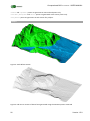
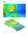
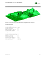
Figure 30: A Delaunay triangulated surface comprising app. 107k faces
ComputationalCAD for AutoCAD provides a Delaunay triangulation algorithm eligible for large scale Digital
Terrain Modelling (DTM). ComputationalCAD for AutoCAD allows to
60

triangulate point data

make lines part of the triangulation

consider holes and islands

reduce the number of vertices of an existing triangulation

generate contour lines of a triangulation
Version 1.5.0
ComputationalCAD for AutoCAD – USER MANUAL
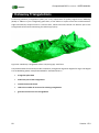
7.1 Theory
A 2d Delaunay triangulation (DT) for a set P of points in the plane is a triangulation such that no point in P
is inside the circumcircle of any triangle in the triangulation. It can be shown that for all possible
triangulations of P, a Delaunay triangulation maximizes the minimum angle of all angles of the triangles in
the triangulation.
Thus, a Delaunay triangulation tends to avoid “skinny” triangles. This property makes it the triangulation
of choice for many purposes, including Digital Terrain Modelling (DTM).
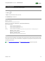
Figure 31: A Delaunay triangulation with all circumcircles and their centres. Image available under GNU
license at http://en.wikipedia.org/wiki/File:Delaunay_circumcircles_centers.png
A Delaunay triangulation is unique in a general case. It is not unique if four triangulation points lie on the
same circle.
A 2d conforming Delaunay triangulation (CDT) is a Delaunay triangulation that respects constraints
(edges). This is done by iteratively inserting additional points (called Steiner points) until no triangle
crosses a constraint.
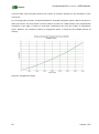
Computational power
In general, triangulating pure point data is much faster than triangulation pure constraint data. This is
because constraints are processed iteratively until no constraint crosses a triangle. Benchmarks for pure
Version 1.5.0
61
ComputationalCAD for AutoCAD – USER MANUAL
constraint data cannot be given because the number of iterations depends on the distribution of the
constraints.
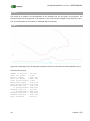
On an average 32bit machine, ComputationalCAD for AutoCAD triangulates about 0.5M to 1M points in
about one minute. This may extend to several millions of points on a 64bit machine. The computational
complexity is On  logn , resulting in near-linear computation time over the number of triangulation
points. However, the maximum number of triangulation points is limited by the available amount of
memory.
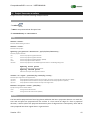
Figure 32: Triangulation timings
62
Version 1.5.0
ComputationalCAD for AutoCAD – USER MANUAL
7.2 Input data
ComputationalCAD for AutoCAD can process the following input data:

Triangulation points are defined as arbitrarily spaced AutoCAD 3d point entities. All triangulation
points will be vertices of the triangles in the CDT.
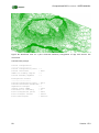
Figure 33: 54k triangulation points

Constraints are defined as an unordered set of non self-intersecting, non-overlapping AutoCAD
3d line entities. The CDT will insert additional points so that no constraint will cross an edge of a
triangle. Thus, spatial constraints become part of the triangulated surface.
Figure 34: 35k contour lines (constraints)

Boundaries are defined as a set of closed, linear AutoCAD polyline entities. Boundary regions may
overlap. Boundaries are not exactly part of the triangulation but will be projected on the
triangulated surface after the triangulation process. The CDT will insert additional points so that
no projected boundary will cross an edge of a triangle. Boundaries allow defining arbitrary shaped
convex or concave holes, islands and outer bounds of the triangulated surface.
Version 1.5.0
63
ComputationalCAD for AutoCAD – USER MANUAL
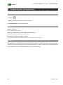
Figure 35: Two closed linear polylines forming two boundary regions
64
Version 1.5.0
ComputationalCAD for AutoCAD – USER MANUAL
7.3 Restrictions
There are following general restrictions:

The triangulation points and constraints must be projectable: a 2d CDT can intrinsically not
triangulate points with identical xy-coordinates or recessing caves. Therefore, triangulation points
with identical xy-coordinates will be removed during the triangulation process. The point with the
highest z-coordinate is kept.
General rule: the CDT can only “see” the xy-projection of the triangulation points and
constraints in UCS. It has no height information during the triangulation process.
Use the CC:POINTS:ELIM2D command to eliminate points with identical xy-coordinates
before triangulating. This keeps your input data clean.

Constraints must not overlap and must not be self-intersecting. Constraints may have identical
start or end points and may be collinear. However, they must not overlap, be self-intersecting or
coincident: since the CDT operates in the UCS xy-plane only, degenerate constraints define overdetermined points along their intersection (i.e. possibly different z-heights at the same xycoordinate).
Use the AutoCAD command _overkill to eliminate overlapping or coincident lines.

Boundaries must be closed and linear. The CDT only accepts closed linear polyline objects as
boundaries. The polylines must exclusively consist of line segments.
Use the AutoCAD command _decurve to linearize a polyline if it does not exclusively consist
of line segments.

Boundaries must lie inside the convex hull of triangulation points and constraints. Boundaries
allow defining arbitrary shaped convex and concave shaped holes, islands and bounds in the
triangulated surface. This implies that boundaries can only be defined where a triangulated
surface exists, precisely being the area inside the convex hull of triangulation points and
constraints.

A Delaunay triangulation is not unique over an evenly spaced rectangular raster. As a
consequence, the direction of the diagonal in a raster may alter when triangulating identical point
data twice depending on the insertion order of the triangulation points.
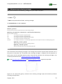
Figure 36: Two valid Delaunay triangulations over a rectangular raster
Version 1.5.0
65
ComputationalCAD for AutoCAD – USER MANUAL
7.4 CDT command
Perform a 2d conforming Delaunay triangulation on a selection of triangulation points, constraints and
boundaries.
Access methods
 Toolbar:
 Menu: ComputationalCAD  Triangulate
 Command entry: CC:CDT
Dialog
Select triangulation points:
Select the triangulation points. This is optional if constraints will be selected. Expects a selection of AutoCAD 3d point entities.
Select constraints:
Select the constraints. Optional if triangulation points have been selected. Expects a selection of non-overlapping AutoCAD 3d line entities. If lines
have been selected, the following dialog occurs:
Number of feasible constraint violations:
Specify the number of feasible edge violations to stop the edge insertion iteration. Expects an integer greater or equal 0.
Default is 0.
Select boundaries:
Select the boundaries (optional). Expects a selection of closed AutoCAD 2d polyline entities.
[The triangulation starts.]
Insert on layer [Current/specify Name] :
<Current>:
The triangles will lie on the current layer. (Default)
<specify Name>:
The following dialog is displayed:
Specify layer name:
Enter the name of the layer the triangles shall be added to. If the layer does not exist, it will be generated.
Insert as block? <Yes, No> :
<Yes>:
The following dialog is displayed:
Specify block name:
Enter the name of the block the triangles shall be added to. If the block does not exist, it will be generated.
<No>:
The triangles will be inserted in the model space. (Default)
Notes
Please read the comments on the input data and the general restrictions.
66
Version 1.5.0
ComputationalCAD for AutoCAD – USER MANUAL
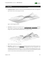
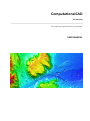
Example
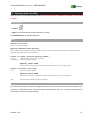
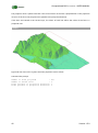
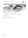
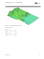
Figure 37: Rendered view on a pure point data Delaunay triangulation of app. 54k points
Command line prompt:
Initial triangulation:
---------------------Initial triangulation points
Initial constraints
Number of boundary regions
Initial boundary segments
:
:
:
:
Triangulation results
--------------------Invalid triangulation points :
Invalid constraints/boundaries:
Degenerate triangles
:
Steiner points added
:
Iterations for conformity
:
Total triangulation points
:
Total triangles created
:
Total time elapsed
:
Version 1.5.0
54327
0
0
0
0
0
0
0
0
54327
107712
2234 ms
67
ComputationalCAD for AutoCAD – USER MANUAL
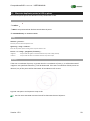
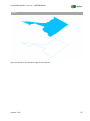
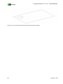
Figure 38: Wireframe view on a pure constraint Delaunay triangulation of app. 45k contour line
constraints
Command line prompt:
Initial triangulation:
---------------------Initial triangulation points
Initial constraints
Number of boundary regions
Initial boundary segments
:
:
:
:
Triangulation results
--------------------Invalid triangulation points :
Invalid constraints/boundaries:
Degenerate triangles
:
Steiner points added
:
Iterations for conformity
:
Total triangulation points
:
Total triangles created
:
Total time elapsed
:
68
0
45347
0
0
45073
2
0
17900
13
63521
126523
12460 ms
Version 1.5.0
ComputationalCAD for AutoCAD – USER MANUAL
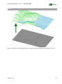
8 Surface reconstruction
ComputationalCAD for AutoCAD allows reconstructing a surface consisting of 3d faces from a wireframe
model consisting of millions of unordered lines.
Version 1.5.0
69
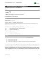
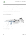
ComputationalCAD for AutoCAD – USER MANUAL
8.1 Reconstruct surface from wireframe command
Reconstruct a surface consisting of triangular and quad 3d faces from a wireframe consisting of unordered
lines.
Access methods
 Toolbar:
 Menu: ComputationalCAD  Reconstruct faces from wireframe
 Command entry: CC:LINES:TOFACES
Dialog
Select lines:
Select the lines
Insert on layer [Current/by Line]:
<Current>:
The faces will lie on the current layer.
<by Line>:
The faces will lie on the layer of the defining lines. (default)
Specify output entity type [All/Triangles only/Quads only]:
<All>:
Both triangular and quad faces will be reconstructed (default).
<Triangles only>:
Only triangular faces will be reconstructed.
<Quads only>:
Only quad faces will be reconstructed.
Specify number of relevant decimal digits <6>:
Specify the number of relevant decimal digits of the coordinates of the start and end point of the lines. Expects an integer between 0 and 12.
Default is 6.
Summary
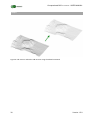
This method identifies all triples and quadruples of connected lines that form a closed triangular or quad
face (“wireframe”). The lines may be completely unordered. The direction of the line may be arbitrary. It
then creates a triangular or quadrilateral AutoCAd 3d face for each identified tuple.
If the insertion layer is ‘byLine’, subsets of lines with the identical layer and colour are built before
reconstructing the surface. Surfaces are then reconstructed for each subset one after another.
The output entity type allows specifying if only triangular, quadrilateral or all identified tuples shall be
considered.
Before reconstructing the surface, the vertex coordinates will be internally rounded to the number of
relevant decimal digits specified.
70
Version 1.5.0
ComputationalCAD for AutoCAD – USER MANUAL
Example
Figure 39: Surface consisting of 3d faces reconstructed from unordered lines
Version 1.5.0
71
ComputationalCAD for AutoCAD – USER MANUAL
9 Convex Hulls and bounding entities
ComputationalCAD for AutoCAD provides several methods to compute 2d and 3d convex hulls of point
clouds. Related to this, it also provides methods to compute minimum enclosing bounding rectangles,
circles and boxes of the convex hulls. This is identical to computing the minimum enclosing bounding
rectangles, circles and boxes of the entire point cloud.
72
Version 1.5.0
ComputationalCAD for AutoCAD – USER MANUAL
9.1 2d convex hull
Compute the 2d convex hull of a point cloud in the plane.
Access methods
 Toolbar:
 Menu: ComputationalCAD  2d convex hull
 Command entry: CC:HULL:2D
Dialog
Select points:
Select the points for which to compute the 2d convex hull.
Specify projection direction [X/Y/Z/Ucs/2Points]:
Select the projection direction.
<X>:
The hull is computed in the global YZ-plane
<Y>:
The hull is computed in the global XZ-plane.
<Z>:
The hull is computed in the global XY-plane (default).
<Ucs>:
The hull is computed in the UCS XY-plane.
<2Points>:
The hull is computed in a user defined plane perpendicular to the projection direction. The following dialog occurs:
Specify first point
Select the first point of the normal vector defining the plane.
Specify second point
Select the second point of the normal vector defining the plane.
Notes
The 2d convex hull is the planar convex polygon that encloses all points with minimum perimeter length.
If the points are 3d points, the 2d convex hull is computed for the projection of these points onto the
specified projection plane.
Use Generate points on primitives and Generate points on solids to generate input data.
Version 1.5.0
73
ComputationalCAD for AutoCAD – USER MANUAL
Example
Figure 40: A 2d convex hull of 24 points
Command line prompt:
Number of vertices on hull : 10
Hull perimeter length
: 2156.6425
Enclosed area in hull plane: 337976.7258
74
Version 1.5.0
ComputationalCAD for AutoCAD – USER MANUAL
9.2 Minimum area enclosing rectangle
Compute the minimum area enclosing rectangle of a point cloud in the plane.
Access methods
 Toolbar:
 Menu: ComputationalCAD  Min. enclosing rectangle
 Command entry: CC:HULL:MINAREA
Dialog
Select points:
Select the points for which to compute the minimum area enclosing rectangle.
Specify projection direction [X/Y/Z/Ucs/2Points]:
Select the projection direction.
<X>:
The rectangle is computed in the global YZ-plane
<Y>:
The rectangle is computed in the global XZ-plane.
<Z>:
The rectangle is computed in the global XY-plane. (default)
<Ucs>:
The rectangle is computed in the UCS XY-plane.
<2Points>:
The rectangle is computed in a user defined plane perpendicular to the projection direction. The following dialog occurs:
Specify first point
Select the first point of the normal vector defining the plane.
Specify second point
Select the second point of the normal vector defining the plane.
Notes
The 2d minimum area enclosing rectangle is the rectangle that encloses all points with minimum area. If
the points are 3d points, the 2d minimum area enclosing rectangle is computed for the projection of
these points onto the specified projection plane. Note that the minimum area enclosing rectangle is not
necessarily identical with the minimum perimeter enclosing rectangle.
Use Generate points on primitives and Generate points on solids to generate input data.
Figure 41: 2d convex hull (green), minimum area enclosing rectangle (red) and minimum perimeter
enclosing rectangle (blue)
Version 1.5.0
75
ComputationalCAD for AutoCAD – USER MANUAL
Example
Figure 42: Minimum area enclosing rectangle of 24 points
Command line prompt:
Minimum perimeter
Width
:
Height
:
Area
:
Perimeter length:
76
enclosing rectangle properties:
682.4514
623.1447
425265.9925
2611.1923
Version 1.5.0
ComputationalCAD for AutoCAD – USER MANUAL
9.3 Minimum perimeter enclosing rectangle
Compute the minimum perimeter enclosing rectangle of a point cloud in the plane.
Access methods
 Toolbar:
 Menu: ComputationalCAD  Min. perimeter rectangle
 Command entry: CC:HULL:MINPERIMETER
Dialog
Select points:
Select the points for which to compute the minimum perimeter enclosing rectangle.
Specify projection direction [X/Y/Z/Ucs/2Points]:
Select the projection direction.
<X>:
The rectangle is computed in the global YZ-plane
<Y>:
The rectangle is computed in the global XZ-plane.
<Z>:
The rectangle is computed in the global XY-plane. (default)
<Ucs>:
The rectangle is computed in the UCS XY-plane.
<2Points>:
The rectangle is computed in a user defined plane perpendicular to the projection direction. The following dialog occurs:
Specify first point
Select the first point of the normal vector defining the plane.
Specify second point
Select the second point of the normal vector defining the plane.
Notes
The 2d minimum perimeter enclosing rectangle is the rectangle that encloses all points with minimum
perimeter length. If the points are 3d points, the 2d minimum area enclosing rectangle is computed for
the projection of these points onto the specified projection plane.
Note that the minimum perimeter enclosing rectangle is not necessarily identical with the minimum area
enclosing rectangle.
Use Generate points on primitives and Generate points on solids to generate input data.
Version 1.5.0
77
ComputationalCAD for AutoCAD – USER MANUAL
Example
Figure 43: Minimum perimeter enclosing rectangle of 24 points
Command line prompt:
Minimum perimeter
Width
:
Height
:
Area
:
Perimeter length:
78
enclosing rectangle properties:
682.4514
623.1447
425265.9925
2611.1923
Version 1.5.0
ComputationalCAD for AutoCAD – USER MANUAL
9.4 Minimum enclosing circle
Compute the minimum enclosing circle of a point cloud in the plane.
Access methods
 Toolbar:
 Menu: ComputationalCAD  Min. enclosing circle
 Command entry: CC:HULL:MINCIRCLE
Dialog
Select points:
Select the points for which to compute the minimum enclosing circle.
Specify projection direction [X/Y/Z/Ucs/2Points]:
Select the projection direction.
<X>:
The circle is computed in the global YZ-plane
<Y>:
The circle is computed in the global XZ-plane.
<Z>:
The circle is computed in the global XY-plane. (default)
<Ucs>:
The circle is computed in the UCS XY-plane.
<2Points>:
The circle is computed in a user defined plane perpendicular to the projection direction. The following dialog occurs:
Specify first point
Select the first point of the normal vector defining the plane.
Specify second point
Select the second point of the normal vector defining the plane.
Notes
The 2d enclosing circle is the circle that encloses all points with minimum diameter. If the points are 3d
points, the 2d minimum enclosing circle is computed for the projection of these points onto the specified
projection plane.
Use Generate points on primitives and Generate points on solids to generate input data.
Version 1.5.0
79
ComputationalCAD for AutoCAD – USER MANUAL
Example
Figure 44: Minimum enclosing circle of 24 points
Command line prompt:
Minimum enclosing
Radius
:
Area
:
Perimeter length:
80
circle properties:
369.4109
428715.4949
2321.0769
Version 1.5.0
ComputationalCAD for AutoCAD – USER MANUAL
9.5 3d convex hull
Compute the 3d convex hull of a point cloud.
Access methods
 Toolbar:
 Menu: ComputationalCAD  3d convex hull
 Command entry: CC:HULL:3D
Dialog
Select points:
Select at least four non-coplanar points for which to compute the 3d convex hull.
Notes
The 3d convex hull of a set of point encloses all points with minimal surface area. The computation of the
3d convex hull requires at least four non-coplanar points (for which the convex hull is a tetrahedron then).
Use Generate points on primitives and Generate points on solids to generate input data.
Example
Figure 45: 3d convex hull of 1000 random points in a cube (wireframe)
Version 1.5.0
81
ComputationalCAD for AutoCAD – USER MANUAL
Figure 46: 3d convex hull of 1000 random point in a cube (rendered)
Command line prompt:
3d convex hull properties:
-------------------------Number of vertices on hull:
Number of invalid vertices:
Number of faces on hull
:
Number of degenerate faces:
Hull surface area
:
Hull volume
:
Center of mass
:
82
140
0
276
0
2487444.0086
287626283.7002
(2114.3216, 1094.4953, 0.0000)
Version 1.5.0
ComputationalCAD for AutoCAD – USER MANUAL
9.6 Principal axes bounding box
Compute the principal axes bounding box of a point cloud.
Access methods
 Toolbar:
 Menu: ComputationalCAD  Principal axes bounding box
 Command entry: CC:HULL:PABB
Dialog
Select points:
Select at least four non-coplanar points for which to compute the principal axes bounding box.
Notes
The principal axes bounding box is the bounding box along the principal axes of inertia of the 3d convex
hull of the point cloud. Along these axes, the minimum extents of the convex hull define the extents of
the bounding box.
In a general case, the principal axes bounding box is a very tight bounding box of a point cloud. However,
tighter bounding boxes may exist. The quality (tightness) of the principal axes bounding box is the better
the more distinct the values of the mass moment of inertia are. In contrast, the principal axes bounding
box may be very poor for example for a cube, which has the same mass moment of inertia about its
centre for any axis.
Use Generate points on primitives and Generate points on solids to generate input data.
Version 1.5.0
83
ComputationalCAD for AutoCAD – USER MANUAL
Example
Figure 47: Principal axes bounding box and convex hull of 195 points
Command line prompt:
Principal axes bounding box properties:
--------------------------------------Width
: 695.3335
Length
: 2144.3264
Height
: 730.5104
Volume
: 1089207088.4633
Center
: (2619.7359, 1095.8920, 0.0000)
First basis vector : (1.0000, 0.0000, 0.0000)
Second basis vector: (0.0000, 1.0000, 0.0000)
Third basis vector : (0.0000, 0.0000, 1.0000)
84
Version 1.5.0
ComputationalCAD for AutoCAD – USER MANUAL
Autodesk, AutoCAD and AutoCAD Mechanical are registered trademarks or trademarks of Autodesk, Inc.,
and/or its subsidiaries and/or affiliates in the USA and/or other countries. All other brand names, product
names, or trademarks belong to their respective holders. Autodesk reserves the right to alter product and
services offerings, and specifications and pricing at any time without notice, and is not responsible for
typographical or graphical errors that may appear in this document. © 2010 Autodesk, Inc. All rights
reserved.
ceometric UG and the ComputationalCAD for AutoCAD software is not affiliated with, endorsed by,
sponsored by, or supported by Autodesk, Inc., and/or its affiliates and/or subsidiaries.
© 2010 ceometric UG. All rights reserved.
Version 1.5.0
85