Download ANTENNA TEST RANGE - Colorado State University

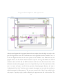
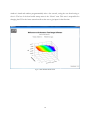
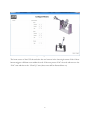
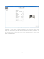
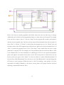
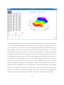
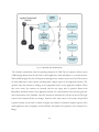
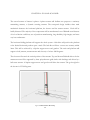
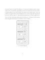
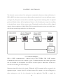
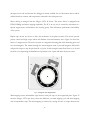
ANTENNA TEST RANGE
First Semester Report
Fall 2009
By
Aaron Kim, Ryan Koenig, Michael Turner
Prepared to partially fulfill the requirements for ECE401
Department of Electrical and Computer Engineering
Colorado State University
Fort Collins, Colorado 80523
Report Approved: ________________________________________________________________
Dr. Branislav Notaros
________________________________________________________________
Olivera Notaros
ABSTRACT
Antenna research has progressed significantly over the past decade, however to conduct any research,
there needs to be one common resource: an antenna test range. This is because of the need to
experiment on physical antennas due to the mathematical complexity of analyzing such antennas
numerically. Such systems that are offered commercially are very expensive and may not come
packaged with features that are important. The primary goal of this project is to create an antenna test
range without the expensive price tag of commercial systems.
For this project, we utilize numerous advanced research tools and knowledge from electromagnetic
theory, antenna measurement theory, RF/microwaves, electronics, communications, computer
hardware, control theory, power analysis, mathematics, computational algorithms, and programming.
Beyond the research required for this project, we will be working on developing a design, analyzing the
design, modeling and simulating our system, programming, building, testing, budgeting, installing, and
assessing on the management and design levels. The design level includes work on the system,
hardware, electronics, and processor levels.
The work that has been done sets the stage for the actual building and testing of the planar scanner
system next semester (Spring 2009). In conjunction with last year’s project, we hope to create a fully
functional antenna test range for use with research and for enhancing curriculum in academic courses.
TABLE OF CONTENTS
Contents
Table of Contents .......................................................................................................................................................i
List of figures ..............................................................................................................................................................ii
Chapter 1: Introduction ........................................................................................................................................... 1
Applications ........................................................................................................................................................ 1
Antenna Measurement Theory ....................................................................................................................... 2
Reflection Ranges ............................................................................................................................................ 2
Free-Space Ranges .......................................................................................................................................... 4
Measurement Methods ................................................................................................................................... 7
Basic System ..................................................................................................................................................... 9
Chapter 4: Antenna Test Software ...................................................................................................................... 11
Initial Development ........................................................................................................................................ 11
Program Architecture ..................................................................................................................................... 12
Program Development and Operation ....................................................................................................... 15
Chapter 3: Test Chamber Monitoring ................................................................................................................ 21
Chapter 4: Planar Scanner ..................................................................................................................................... 24
Chapter 5: Electronics............................................................................................................................................ 26
Chapter 6: Future Work ........................................................................................................................................ 29
Programming .................................................................................................................................................... 29
Mechanical Design and Analysis................................................................................................................... 29
Electronics ........................................................................................................................................................ 29
Appendix 1: Budget ................................................................................................................................................ 30
Bibliography ............................................................................................................................................................. 31
i
LIST OF FIGURES
Figure 1:
Figure 2:
Figure 3:
Figure 4:
Figure 5:
Figure 6:
Figure 7:
Figure 8:
Figure 9:
Figure 10:
Figure 11:
Figure 12:
Figure 13:
Figure 14:
Figure 15:
Figure 16:
Figure 17:
Figure 18:
Figure 19:
Figure 20:
Figure 21:
Figure 22:
Figure 23:
Figure 24:
Figure 25:
Figure 26:
Figure 27:
Near Field Radiation of Cell Phone Near Human Head ............................................................ 1
Geometrical Arrangement for a Reflection Range ....................................................................... 3
Geometrical Arrangement of an Elevated Range ......................................................................... 4
Geometrical Arrangement of a Slant Range .................................................................................. 5
Configuration of a CATR.................................................................................................................. 6
Inside an Anechoic Chamber ........................................................................................................... 7
Field Regions ....................................................................................................................................... 8
Example Test System ......................................................................................................................... 9
Scanning Methods............................................................................................................................. 10
Antenna Software Prototype ...................................................................................................... 12
Program functions and states ..................................................................................................... 13
State Diagram ................................................................................................................................ 14
Initialize State ................................................................................................................................ 15
User interface home screen ........................................................................................................ 16
Configure motors screen ............................................................................................................. 17
Configure VNA screen ................................................................................................................ 18
Run Measurement Sub-VI .......................................................................................................... 19
Display data screen ....................................................................................................................... 20
Flowchart of the Camera System............................................................................................... 22
Example Image from Camera Software ................................................................................... 23
Planar Scanner Sketch Up ........................................................................................................... 24
Polarization Sketch Up ................................................................................................................ 25
Flowchart of Electronics ............................................................................................................. 26
Diagram of the Stepper Motor .................................................................................................. 27
Two Possible Types of Outputs From Motor Driver ........................................................... 28
Graph of PWM Signal ................................................................................................................. 28
Expected Budget........................................................................................................................... 30
ii
CHAPTER 1: INTRODUCTION
Due to the high saturation of electronics in today’s society, antenna research is an immensely hot
topic. Just in one day, the number of times an average person uses an antenna is staggering. This is all
the motivation needed to foray into antenna research. This chapter discusses the need for antenna
research and presents current applications of such research.
Applications
One recent application of antenna research that has received a dosage of media coverage is the cell
phone and brain tumor link. Using antenna test ranges as well as simulation software, this topic has
been researched extensively; however the research is still inconclusive. Using the test chamber, we can
measure the strength of the signal coming from a cell phone and deduce the possible biological effects
it may have on the human body. This can also be done for other electronics as well.
Figure 1: Near Field Radiation of Cell Phone Near Human Head
1
With consumer electronics becoming smaller and smaller yet demanding a connection to the digital
world, it is no wonder there is an emphasis on the research and development of newer, smaller, more
reliable antennas. These can be applied in almost any modern day electronic device such as Global
Positioning System (GPS) devices, smart phones, portable computing, wireless networking, Radio
Frequency Identification (RFID), and many more. Each of the antennas developed for these devices
required extensive testing to ensure the quality of the signal transmitted and received.
Antenna Measurement Theory
Oftentimes, antennas are very complex. This poses a problem for analyzing antennas as the
mathematical computations are very complex as well. It is very impractical, in terms of time spent, to
take on the analysis of an antenna. As a remedial solution, simulation software has been created to
model these antennas. Unfortunately, the software available for simulating antennas is based on theory
and because antennas are breaking new ground every few months, we are not entirely sure if the
theoretical models are accurate. Therefore, we need to test the antenna in a test range. By physically
testing the antenna and measuring the behavior, we can analyze the results more accurately and with
much more speed.
To perform an antenna test, we must have an antenna test range. Which test range we want to use is a
tricky question. There are many types of test ranges and each offer benefits as well as shortcomings.
Determining which test range to use is crucial to getting a good test. Below, you will find two main
types of ranges and a brief analysis on their benefits and shortcomings.
REFLECTION RANGES
This is one of the two basic types of ranges. A reflection range is useful for creating a “quiet zone” in
the region of the test antenna. Figure 2 shows the geometrical arrangement for such a range. As you
can see, the signal is reflected off the ground. This is a design constraint that is unique to each
reflection range. This type of range is useful for understanding the reflective quality of antennas and
also accommodates antennas that operate in the Ultra High Frequency (UHF) range.
2
Figure 2: Geometrical Arrangement for a Reflection Range
The downside to using reflection range is choosing the right location to place one of these ranges. This
range is susceptible to inclement weather in the general area, a common problem with outdoor ranges.
Also, this type of range needs to be installed in a location with a smooth uniform ground in order to
get the intended reflection. This type of range is especially prone to interference from the surrounding
environment.
3
FREE-SPACE RANGES
Unlike the reflection range, a free-space range aims to decrease contributions from the environment.
This accomplished through several methods which vary.
Elevated Ranges
This type of range is very similar to a reflection range; however this type of range is used to test very
large antennas. The antennas are usually mounted atop a tall building with a clear line-of-sight to the
source antenna. Again, these types of ranges are susceptible to inclement weather as these antennas are
usually too large to place indoors. Another downside is the need for a tall tower or building and a large
test area. Figure 3 shows the geometry of this type of range.
Figure 3: Geometrical Arrangement of an Elevated Range
Slant Range
A slant range places the source antenna close to the ground while the test antenna is placed on top of a
tower. It is best to make the tower out of nonconducting materials in order to suppress reflections
from the tower. This type of system requires less real estate than an elevated range. However, it is
important to have a smooth ground surface to prevent any reflections from the ground. Again, this
type of arrangement is susceptible to outdoor weather.
4
Figure 4: Geometrical Arrangement of a Slant Range
Compact Antenna Test Range (CATR)
This type of range utilizes a reflector that reflects a signal towards the test antenna. The reflector is
specially built so the reflected signal becomes a plane wave field without having to cover a large
distance. This satisfies the far-field criteria in a small space. This is an extremely useful way to test the
far-field characteristics inside a small chamber. The downside is getting a reflector. The reflector
cannot have a smooth edge and instead must have a serrated edge. This is to suppress the diffraction
that occurs. Also, the reflector must be large and parabolic with a strong enough mount to keep it
stable.
5
Figure 5: Configuration of a CATR
Anechoic Chambers
Last, but certainly not least, is the anechoic chamber. This type of test range is kept indoors where the
walls are covered in absorber material. This material suppresses the reflected waves to keep the
measurement isolated. The absorber material is also shaped like a pyramid to prevent any diffractive
waves from reflecting. Also, to prevent any environmental noise, a layer of conductive material should
be laid out underneath the absorber material. This creates a Faraday Cage inside the chamber. An
anechoic chamber is useful for providing a silent room as well as enough space to perform far field
measurements. Unfortunately, the absorber materials are expensive along with finding a large enough
room for these experiments. Finally, it is worth mentioning that this project utilizes an anechoic
chamber and all the developments we have made are to outfit this anechoic chamber.
6
Figure 6: Inside an Anechoic Chamber
MEASUREMENT METHODS
To perform a measurement, assuming all the conditions for a measurement are satisfied, we must
choose what kind of measurement we want to perform. There are two distinct categories: near field
and far field.
Near Field
There are two subregions in the near field region: reactive near field and radiating near field.
The reactive near field region is the region in which we are interested in the reactive element of the
travelling wave. This is because the reactive element is much greater than the radiating element.
Other than the reactive field, there is the radiating field. In this region, also called the Fresnel Region,
the radiation fields dominate and angular field distribution depends on the distance from the antenna.
7
Far Field
This region is usually the region most antenna research is based around. In this region, we can assume
the radiation pattern is independent of the distance from the antenna. This is because at a large enough
distance, the travelling wave emitted from an antenna appears to look like a plane wave.
Figure 7: Field Regions
8
BASIC SYSTEM
Now that we have established a large chunk of the theory, we must now discuss the basic setup of a
system. To begin, we have to establish the basic elements: a source antenna and a test antenna.
According to the reciprocity rule, the antenna we want to test can be on the source side or the
measurement side. However, it is conventional to place the antenna under test (AUT) on the
measurement side. Figure 8 shows what we mean by source and test.
Figure 8: Example Test System
9
The test antenna positioning system is usually one of three types: a planar, spherical, or cylindrical
scanner. We want to use one of these systems so that when we analyzed the measurement results, we
can simplify the mathematics. In Figure 9, you can see the three different scanning methods. Every dot
in the picture is roughly a point where the antenna takes a measurement. Of course, the positions can
be even finer in detail, but that is entirely a decision for you to make.
Figure 9: Scanning Methods
10
CHAPTER 4: ANTENNA TEST SOFTWARE
Initial Development
To control the antenna positioning system, a complex software application needed to be developed.
The previous year’s team developed a prototype of this software using C# and Visual Studio. Shown
below is the GUI (Graphical User Interface) for this prototype, which allows the user to interface with
the system and configure measurements. However, this prototype lacked the ability to configure and
load calibration files from the VNA (Vector Network Analyzer). Additionally, the software did not
allow the user to configure sweep measurements along multiple axes. These among other small issues
lead to the software being redeveloped using National Instruments LabView 8.6. Being a test and
measurement based software; LabView was an ideal choice for this application and ultimately lead to
significant cuts in development time. So exactly what is LabView one might ask? To answer this, one
has to think of writing code in an entirely new way. Normally when a programmer sits down and
begins writing a piece of code, they begin to typing line after line of code. In LabView however, the
code is graphical not text based, so a LabView developer would sit down and begin creating a block
diagram, not lines of text. This is the fundamental difference between other languages like C# and
LabView. This difference enables the programmer to see the program visually and in many cases
increases the speed of development.
11
Figure 10: Antenna Software Prototype
Program Architecture
The first task of development is to choose a program architecture that best matches the application. In
order to accomplish this task, it is necessary to know what the desired functions of the software are to
be, what other devices or programs the software will communicate with, and what speed requirements
must the software meet. These among other requirements and specifications are important factors in
choosing the overall architecture of the software. For this application, the following factors were
important when choosing the correct architecture.




RS232 communication with the custom motor driver PCB
TCP-IP communication with the VNA
Fast enough to process gain information from the VNA while scanning
User interface with moderate functionality
o Must support user options
o Allow for data to be exported
12
Considering these factors, it was decided that the best program architecture for this system would be
an event bases state machine. A state machine allows for the code to be easily expanded upon, while
keeping it fast enough to process large amounts of data quickly. Moreover, support for events gives
the user a great amount of functionally in the GUI. The next step in the development process was to
determine what states would be necessary in order to meet the project specifications. The figure below
shows what functions the software needs to perform and what states are necessary to perform each
specified function. As seen in the figure, most of the states within the program are used in the program
utilities section which is responsible for all connections, error logging, and closing all references when
done.
Figure 11: Program functions and states
With the required states now determined, the next step is to figure out what order each of these states
should be called. This is accomplished by creating a state diagram which indicates the top level
program flow and allows the programmer to begin coding the framework of the application. Another
key aspect to consider when creating the state diagram is the GUI design. For this application we
decided to use a wizard type GUI in order to simplify measurement configuration. The wizard GUI
asks for certain parameters from the user and chooses the next screen based on those parameters. For
13
example anyone who has set up a printer on their home computer most likely encountered a wizard
asking for parameters on multiple screens. This is another key difference between the new application
and the previously developed prototype, which had a traditional GUI. Shown in the figure below is the
state diagram for the application. From the “start” position on the diagram one can trace their way
through the different states of the program. After the first four states (the yellow states) execute
automatically on program startup, the code will stop and wait for user input. When the user has
finished inputting their desired parameters and clicks for example “next” it triggers an event in the
code. When the “next” button is pushed, the code wakes up and grabs the user input parameter and
chooses the next state based on these parameters. From the state diagram, for example, in order to exit
the program it is necessary to return to the home state and then choose exit. Using the state diagram,
the software framework was then generated reflecting an equivalent program flow. The framework
within the code is the state machine itself and its supporting VI’s.
Figure 12: State Diagram
14
Program Development and Operation
Figure 13: Initialize State
After the state diagram and the program framework were complete, the real coding was ready to take
place. The figure below shows the overall frame work of the application and the “Initialize” state. As
in the state diagram the first state the code operates is the “Initialize” state. Within this state the
program retrieves the file structure location needed to open the error log and initializes the TCP-IP
connection with the VNA and the RS232 connection with the motor driver board. Once all the
information is retrieved the program moves to the “Open Error Log” state. The only function of this
state is to create and open a text file in the previously obtained program directory and name it
“Administrative Error Log.” Once that state is complete the program can now track and record errors
within the program for debug purposes. The next state executed is the “About” state, which has the
sole purpose of opening a pop-up window displaying the program name and version number. The
15
window is timed and vanishes programmatically after a few seconds, saving the user from having to
close it. The last of the hard coded startup states is the “Home” state. This state is responsible for
changing the GUI to the home screen that allows the user to give input for the first time.
Figure 14: User interface home screen
16
Figure 15: Configure motors screen
The home screen of the GUI shown below has two buttons in the lower right corner. Each if these
buttons triggers a different event within the code. If the user presses “Exit” the code with move to the
“Exit” state and then to the “Clean Up” state (these states will be discussed later on).
17
Figure 16: Configure VNA screen
Alternatively, if the user presses “Configure Measurement” the code moves to the “Motor Sweep
Setup” state. This state, among other small tasks changes the GUI to the configure motors screen. On
this screen the user has the ability to input all the necessary information needed to create a sweep
pattern for the measurement.
18
Figure 17: Run Measurement Sub-VI
Each of the boxes are already populated with default values that user can either keep or change.
Additionally, each of the boxes has programmatic limits as to what values can be entered. For example
if the user tries to input a value of -1 into the “Steps” box the program will override it and replace it
with the closest acceptable value. Once the user has entered all the information they have the option to
select “Next” or “Home.” If “Home” is selected then then program moves to the “Home” state and
the home screen of the GUI reappears upon which the user again has the choices described above. If
“Next” is pressed the program moves to the “VNA Setup” screen which allows the user to input
parameters to setup the VNA. For example, one of the parameters that the user has the ability to select
is the calibration file. For more information on calibrating the VNA for your specific measurement
please read Agilent’s user manual for the device. In the VNA setup screen is shown below, the user
has the option once again to click “Home” or if the user wishes to continue “Run Measurement.” If
the user selects “Run Measurement” the code moves to the “Run Measurement” state and changes the
GUI screen to scan in progress. Within this state is a Sub-VI containing a state machine of its own,
responsible for sending commands to the motors, moving them to the proper locations, and then
requesting a measurement from the VNA.
19
Figure 18: Display data screen
The “Run Measurement” Sub-VI receives the measurement data back from the VNA before moving
to the next measurement location. After this Sub-VI is done executing, the program moves to the
“Array to Listbox” state. In is in this state where the program transforms the 2-dimensional array of
data compiled received from the motor driver PCB and the VNA and transforms it into a MultiColumn Listbox, which is easy for the user to interact with. Additionally, at once this state is finished
executing, GUI is switched to the data display screen (shown above). This screen allows the user to see
all the data generated by the scan as well as the sweep settings previously defined. On the right is as a
three dimensional model showing the data for one particular frequency. The model is interactive,
meaning the user can zoom in or out and move it around. Additionally, the user can select the
frequency displayed on the graph by double clicking a frequency in the data table. However, most of
the time it will be for useful for the user to export the data to another analysis program such as Matlab.
These can be accomplished by selecting the “Export Data” button on the left side beneath the data
table. If the user wishes to take another measurement, the “home” button will take the program back
to the home screen where the program can either be exited or a new measurement can be started.
20
CHAPTER 3: TEST CHAMBER MONITORING
Radiation within the anechoic chamber and moving equipment create an environment that is
dangerous for humans. In order to observe the antenna testing experiments, cameras will be placed in
the test chamber. This allows the test operators to verify the orientation of the various scanners and
know if emergency shutoff is needed. Both transmitter and receiver antennas will be monitored using
two Logitech QuickCam® Orbit AF webcams. This camera was chosen because of the shaft
extension, high resolution and light management. The shaft extension is the most important feature.
The long shaft will allow the base of the camera to be shielded by anechoic foam which should reduce
the interference with the test. Once the test chamber is functional, the amount of camera interference
will be analyzed and changes with the camera mounting will be investigated and improved if needed.
The standard software provided by the camera does not support the viewing of two cameras in the
same application. This required a small application to be written that will display both camera images
on the same screen with simplified controls for turning on both cameras. This camera application will
be referred to as ATRCamApp. The programming of the application implements Microsoft
DirectShow tools and was written in C++ .NET using Microsoft Visual Studio.
21
Figure 19: Flowchart of the Camera System
The Cameras communicate with the operating computer via USB. The test operator will then open
ATRCamApp directly from the LabView Control application, which will display on a second monitor.
When ATRCamApp loads, the COM ports containing the two camera sources are found. The sources
are then initialized for video capture and designated a display panel on the application window. The
operator starts the cameras by clicking on the appropriate button on the application window. When
this event occurs, the cameras are powered and the raw image data is gathered, filtered with
DirectShow and made visible on the application window. No other functions were necessary given the
static environment of the Chamber. Once the cameras are mounted, they will not be moved. The light
source in the chamber will also not change. Because of the static nature of the system, the provided
Logitech software can be used to initially configure the cameras for enhanced capture response. This
small application with its simplicity and accessibility will enhance the operation of the Antenna Test
Range.
22
Figure 20: Example Image from Camera Software
23
CHAPTER 4: PLANAR SCANNER
The second scanner of interest is planar. A planar scanner will facilitate two purposes: a stationary
transmitting antenna, a dynamic scanning antenna. The conceptual design includes three main
mechanical elements: the horizontal platform, the elevator and the antenna mount. Each will be
briefly discussed. The majority of the components will be manufactured out of Delrin® acetal because
of its low friction coefficient, ease of precision manufacturing, long durability, high integrity and most
very low conductance.
The horizontal sliding platform will support the whole system. A belt drive will position the platform
at the desired horizontal position upon a track. The belt drive will have a worst case accuracy within
2mm. This will be achieved by a bipolar stepper motor and gearbox. The track and platform will
support a load (antenna, antenna mount and elevator) of at least 100 kilograms.
The elevator will control the vertical position of the antenna. Top and bottom Delrin® shelves for the
antenna mount will be supported by three polycarbonate guide shafts with bushings and driven by a
ball screw actuator. A bipolar stepper motor and gear box will drive the actuator. The goal weight for
the elevator is 25-30 kilograms.
Figure 21: Planar Scanner Sketch Up
24
The antenna mount will control the polarization of the antenna. The spherical scanner is using a
stepper motor to accomplish this. The drawbacks of the motor occurs when the connecting the cables
to adapter positioned on the center backside of the antenna and the stepper motor is heave and
conductive. The planar scanner will use a small plastic linear scanner to push a right angle arm that
pivots at its vertex (see Figure 13). This method will be much more cost effective, lighter and less
noisy in the system while still providing rotation for polarization up to 200 degrees. Other mounting
plates and supports will be designed to accommodate a variety of antennas.
Figure 22: Polarization Sketch Up
25
CHAPTER 5: ELECTRONICS
The electronic system consists of four main parts: communication between software and circuitry via
USB to RS232, the micro processor, motor driver and movement device i.e. motor and linear actuator.
(see Figure 23). The planar scanner will be controlled using electronics remaining from the spherical
positioned. Similar circuitry will be implemented because of the identical parts except for controlling
the electrical linear actuator for the antenna mount. The printed circuit board layout will be designed
using the freeware application CadSoft Eagle. While commercial electronic systems are available, none
will offer the custom design needed at a cost effective price.
Figure 23: Flowchart of Electronics
USB to RS232 communication is achieved using FTDI FT232RL USB UART interface.
Communication will occur as the controller is given a command and when the control reports back
that the command was accomplished. The LabView software requires a 28800 baud. ASCII will be
sent and received through a virtual serial port.
Microprocessing will be done by the Atmel ATMega168. ASCII commands will be converted to the
appropriate signals to motor driver IC and linear actuator. We continue to use the ATMega168 to
reduce writing new code for the electronics, the free application WinAVR to compile the
26
microprocessor code and because the debugger is already available for use. Movement devices will be
enabled based on counters and comparators contained in the microprocessor.
Motor driving is managed with the Allegro A3970 IC device. This motor driver is equipped with
PWM, H-Bridge and micro stepping capabilities. The IC is an easy way to control the movement of a
bipolar stepper motor and minimizes the circuitry greatly. This will increase performance and stability
of the system.
Bipolar step motors are chosen to drive the mechanics of the planar scanner. The motors provide
precise control and high torque which will eliminate some measurement error. Figure 24 shows the
basics of a stepper motor. The motor consists of a magnetized rotating plate with alternating poles and
two electromagnets. The current through the electromagnets create a powerful magnetic field which
will provide torque to step the plat from N to S poles. In this example current flows from 1a to 1b and
from 2b to 2a. Sequencing the distribution of potential to the 4 ports will make the motor rotate.
Figure 24: Diagram of the Stepper Motor
Microstepping creates intermediate steps between each pole step on the magnetized plate. Figure 25
from the Allegro A3979 spec sheet, shows the difference a normal stepping cycle and microstepping
with 4 intermediate steps. The microstepping is achieved by varying the ratio of torque between the
27
two phases in a sinusoidal cosinusoidal method. Microstepping provides a much higher resolution of
stepping, but there is a trade off of accuracy for each intermediate step.
Figure 25: Two Possible Types of Outputs From Motor Driver
Pulse width modulation (PWM) is used to accelerate the motor and then to regulate the speed of the
motor. The duration of the pulse high time will determine the average voltage applied to the motors
which the motor torque is proportional (see Figure 26). Torque determines the speed at which the
motor turns or slows down. The motor driver IC will automate this signal.
Figure 26: Graph of PWM Signal
28
CHAPTER 6: FUTURE WORK
Next semester, we plan on continuing with the progress that we have made this semester. The
following is a brief list of items we plan to accomplish.
Programming
This semester, we created a LabView program that acts as the control center, combining information
sent to and from the microprocessor and the Vector Network Analyzer. Next semester, we hope to
expand that program to give us control of the planar scanner.
We also want to reprogram the microprocessor code to decrease the size and efficiency of the code.
We also want to take a look into a finer motor movement that gives us the ability to move two motors
at once.
Mechanical Design and Analysis
We plan on creating a CAD design of the planar scanner that we plan on using to simulate stresses and
other dynamic tests on the planar scanner. Doing so will give us confidence in the design we came up
with this semester. Also, we need to order the parts needed and get them machined.
Electronics
We hope to create a new printed circuit board (PCB) next semester that will house all the motor
control electronics.
29
APPENDIX 1: BUDGET
This semester we focused on research and software design. The school provided the developmental
software used. The only expense was due to electronics research with breadboard and components.
Planar
These expenses are covered by the funding given to all senior design students.
Description
Quantity
Estimated Price
Actual Price
PCB Board
1
$50
-
PBC Components
Multi
$100
-
Machined Delrin
Multi
$1,000
-
Fasteners
Multi
$200
-
Screw Drive
1
$300
-
Belt Drive
1
$200
-
Linear Actuator
1
$100
-
Multi
$200
-
Antenna Mounting Plate
1
$10
-
Shaft Extention
1
$35
-
Anodizing Positioner
1
$150
-
Shelf Plate
1
$200
-
Breadboard
1
$0
Multi
$65
BBoard
Spherical
Misc. Costs
Breadboard Componets
Total:
$2,545
Figure 27: Expected Budget
30
$65
BIBLIOGRAPHY
Stutzman, Warren L., Thiele, Gary A.. Antenna
Theory and Design, Second Edition. John Wiley
& Sons,1998.
Balanis, Constantine. Antenna Theory: Analysis and
Design, Second Edition. John Wiley & Sons,
1997.
ORBIT/FR. Antenna Measurement Theory.
ORBIT/FR, 2003.
Allegro Microsystems. A3979: Microstepping
DMOS Driver with Translator. Allegro, 2008.
Agilent Technologies. PNA Series Programming
Information and Examples. Agilent
Technologies, 2009.
31
4