Download SandMath

SandMath_44 Manual 6$1'0$7+B
0DWK([WHQVLRQVIRUWKH+3
User’s Manual and Quick Reference Guide Written and programmed by Ángel M. Martin November 2012 (c) Ángel M. Martin Revision 44_E Page 1 SandMath_44 Manual This compilation revision 4.44.44 (really!)
Copyright © 2012 Ángel Martin
Acknowledgments.Documentation wise, this manual begs, steals and borrows from many other sources – in particular
Jean-Marc Baillard’s program collection on the web. Really both the SandMath and this manual would
be a much lesser product without Jean-Marc’s contributions.
There are multiple graphics and figures taken from Wikipedia and Wolfram Alpha, notably when it
comes to the Special Functions sections. I’m not aware of any copyright infringement, but should that
be the case I’ll of course remove them and create new ones using the SandMath function definition and
PRPLOT. Just kidding...
Original authors retain all copyrights, and should be mentioned in writing by any party utilizing this
material. No commercial usage of any kind is allowed.
Screen captures taken from V41, Windows-based emulator developed by Warren Furlow.
See www.hp41.org
SandMath Overlay © 2009 Luján García
Published under the GNU software licence agreement.
(c) Ángel M. Martin Revision 44_E Page 2 SandMath_44 Manual Table of Contents. - Revision E.
1. Introduction.
Function Launchers and Mass key assignments
Used Conventions and disclaimers
Getting Started. Accessing the functions.
Main and Dedicated Launchers: the Overlay
Appendix 1.- Launcher Maps
Function index at a glance.
7
8
9
10
11
12
2. Lower Page Functions in Detail
2.1. SandMath44 Group
Elementary Math functions.
Number Displaying and Coordinate conversions
Base Conversions
First, Second and Third degree Equations
Appendix 2.- FOCAL program listing
Additional Test Functions: rounded and otherwise
15
17
18
19
21
22
2.2. Fractions Calculator
Fraction Arithmetic and displaying
23
2.3. Hyperbolic Functions
Direct and Indirect Hyperbolics
Errors and Examples
25
26
2.4. Recall Math
Individual RCL Math functions
RCL Launcher – the “Total Rekall”
Appendix 3.- A trip down memory lane
27
28
29
3. Upper Page Functions in Detail
3.1 Statistics / Probability
Statistical Menu – Another type of Launcher
Alea jacta est…
Combinations and Permutations
Linear Regression – Let’s not digress
Ratios, Sorting and Register Maxima
Probability Distribution Function
And what about Prime Factorization?
Appendix 4. Prime Factors decomposition
Distance between two Points.
(c) Ángel M. Martin Revision 44_E 31
32
33
34
35
36
37
38
40
Page 3 SandMath_44 Manual 3.2. Factorials
A timid foray into Number Theory
Pochhammer symbol: rising and falling empires
Multifactorial, Superfactorial and Hyperfactorial
Logarithm Multi-Factorial
Appendix 5.- Primorials; a primordial view.
41
42
43
45
46
3.3. High-Level Math
The case of the Chameleon function in disguise
49
Gamma Function and associates
Lanczos Formula
50
51
52
53
53
54
55
56
56
Appendix 6. Comparison of Gamma results
Reciprocal Gamma function
Incomplete Gamma function
Logarithm Gamma function
Digamma function
Euler’s Beta function
Incomplete Beta function
Bessel Functions and Modified
Bessel functions of the 1st Kind
Bessel functions of the 2nd Kind
Getting Spherical, are we?
Programming Remarks
57
57
58
59
60
63
Riemann Zeta Function
64
66
67
Appendix 7. FOCAL program for Yn(x), Kn(x)
Appendix 8.- Putting Zeta to work: Bernoulli numbers
Lambert W Function
3.4. Remaining Special Functions in Main FAT
Exponential Integral and associates
Errare humanum est…
The unsung Hero
Appendix 9.- Inverse Error function: coefficients galore
How many logarithms, say what?
Fourier Series
Appendix 10. Fourier Coefficients by brute force
69
71
71
72
73
74
76
3.5. More Special Functions in Secondary FAT
3.5.1. Carlson Integrals and associates: The Launcher
The Elliptic Integrals
Carlson Symmetric Form
Airy Functions
Fresnel integrals
Weber and Anger Functions
(c) Ángel M. Martin Revision 44_E 77
78
79
80
81
Page 4 SandMath_44 Manual 3.5.2. Hankel, Struve and others: The Launcher
A Lambert relapse
Hankel functions – yet a Bessel 3rd. Kind
Getting Spherical, are we?
Struve Functions
Lommel functions
Lerch Trascendent function
Kelvin functions
Kummer Functions
Associated Legendre functions
Toronto Function
Poisson Standard Distribution
3.5.3. Orphans and Dispossessed.
Tackle the Simple ones First
Debye Function
Dawson Integral
Hypergeometric Functions
Integrals of Bessel functions
Appendix 11.- Looking for Zeroes
.END.
(c) Ángel M. Martin Revision 44_E 82
83
83
85
86
87
88
89
90
91
91
92
93
94
95
96
97
98
Page 5 SandMath_44 Manual Note: Make sure the revision “G” (or higher) of the Library#4 module is installed.
(c) Ángel M. Martin Revision 44_E Page 6 SandMath_44 Manual SandMath_44 Module – Revision E
Math Extensions for the HP-41 System
1. Introduction.
Simply put: here’s a compilation of (mostly MCODE) Math functions to extend the native function set of
the HP-41 system. At this point in time - way over 30 years after the machine’s launch - it’s more than
likely not realistic to expect them to be profusely employed in FOCAL programs anymore - yet they’ve
been included for either intrinsic interest (read: challenging MCODE or difficult to realize) or because of
their inherent value for those math-oriented folks.
This module is an 8k implementation. The first 4k includes more general-purpose functions, re-visiting
the usual themes: Fractions, Base conversion, Hyperbolic functions, RCL Math extensions, as well as
simple-but-neat little gems to round off the page. In sum: all the usual suspects for a nice ride time.
The second page delves into deeper territory, touching upon the special functions field and
Probability/Statistics. Some functions are plain “catch-up” for the 41 system (sorely lacking in its native
incarnation), whilst others are a divertment into a tad more complex math realms. All in all a mixedand-matched collection that hopefully adds some value to the legacy of this superb machine – for many
of us the best one ever.
I am especially thankful for the essential contributions from Jean-Marc Baillard: more than 3/4ths of
this module are directly attributable to his original programs, one way or another.
Wherever possible the 13-digit OS routines have been used throughout the module – ensuring the
optimal use of the available resources to the MCODE programmer. This prevents accuracy loss in
intermediate calculations, and thus more exact results. For a limited precision CPU (certainly per today’s
standards) the Coconut chip still delivers a superb performance when treated nicely.
The module uses routines from the Page#4 Library (a.k.a. “Library#4”). Many routines in the library
are general-purpose system extensions, but some of them are strictly math related, as auxiliary code
repository to make it all fit in an 8k footprint factor - and to allow reuse with other modules. This is
totally transparent to the end user, just make sure it is installed in your system and that the revisions
match. See the relevant Library#4 documentation if interested.
Function Launchers and Mass key assignments.
As any good “theme” module worth its name, the SandMath has its own mass-Key assignment routine.
Use it to assign the most common functions within the ROM to their dedicated keys for a convenient
mapping to explore the functions. Besides that, a distinct feature of this module is the function
launchers, used to access diverse functions grouped by categories. These include the Hyperbolic, the
Fractions, the RCL Math, and the Special Function groups. This saves memory registers for key
assignments, whilst maintaining the standard keyboard available also in USER mode for other purposes.
This is the fourth incarnation of the SandMath project, which in turn has had a fair number of revisions
and iterations on its own. The new distinct addition has been a secondary Function address Table (FAT)
to provide access to more functions, exceeding the limit per page imposed by the operating system.
Some other refinements consisted in a rationalization of the backbone architecture, as well as a more
modular approach to each of pages of the module. Gone are the “8k” vs. “12k” distinctions of the past
– as now the Matrix and Polynomial functions have an independent life of their own in separate
modules - more on that to come.
This manual is a more-or-less concise document that only covers the normal use of the functions.
(c) Ángel M. Martin Revision 44_E Page 7 SandMath_44 Manual Conventions used in this manual.
All throughout this manual the following convention will be used in the function tables to denote the
availability of each function in the different function launchers:
[*]:
[ΣF]:
[H]:
[F]:
[RC]:
[CR];
[HK]:
[ΣΣ]:
[Σ$]:
assigned to the keyboard by
direct execution from the main launcher
executed from the hyperbolics launcher
executed from the fractions launcher
executed from the RCL# launcher,
executed from the Carlson Launcher
executed from the Hankel launcher
executed from the Statistics Menu,
sub-function in the secondary FAT.
HMKEYS
ΣFL
-HYP
-FRC
-RCL
(no separate function exists)
(no separate function exists)
–ST/PRB
ΣFL$
HMKEYS uses the value in X as a flag to decide whether to assign or to remove the mass key
assignments. If x=0 the assignments will be removed, any other value will make them. There are a
total of 25 functions assigned, refer to the SandMath overlay for details.
Note for Advanced Users:
Even if the SandMath is an 8k module, it is possible to configure only the first (lower) page as an
independent ROM. This may be helpful when you need the upper port to become available for other
modules (like mapping the CL’s MMU to another module temporarily); or permanently if you don’t care
about the High Level Math (Special Functions) and Statistics sections.
Think however that the FAT entries for the Function launchers are in the upper page, so they’ll be gone
as well if you use the reduced foot-print (4k) version of the SandMath.
Upper Page:
High-Level Math, Stats,
Function Launchers
Lower Page:
SandMath_44, FRC, HYP,
RCL# Math
Note that it is not possible to do it the other way around; that is plugging only the upper page of the
module will be dysfunctional for the most part and likely to freeze the calculator– do not attempt.
Final Disclaimer.With “just” an EE background the author has had his dose of relatively special functions, from college
to today. However not being a mathematician doesn’t qualify him as a field expert by any stretch of the
imagination. Therefore the descriptions that follow are mainly related to the implementation details,
and not to the general character of the functions. This is not a mathematical treatise but just a
summary of the important aspects of the project, highlighting their applicability to the HP-41 platform.
(c) Ángel M. Martin Revision 44_E Page 8 SandMath_44 Manual Getting Started: Accessing the Functions.
There are about 160 functions in the SandMath Module. With each of its two pages containing its own
function table, this would only allow to index 128 functions - where are the others and how can they be
accessed? The answer is called the “Multi-Function” groups.
Multi-Functions ΣFL# and ΣFL$ provide access to an entire group of sub-functions, grouped by their
affinity or similar nature. The sub-functions can be invoked using either its index within the group,
using ΣFL#, or its direct name, using ΣFL$. This is implemented in such a way that they are also
programmable, and can be entered into a program line using a technique called “non-merged
functions”.
You may already be familiar with this technique, originally developed by the HEPAX programmers. In
the HEPAX there were two of those groups; one for the XF/M functions and another for the HEPAX/A
extensions. The PowerCL Module also contains its own, and now the SandMath joins them – this time
applied to the mathematical extensions, particularly for the Special Functions group.
A sub-function catalog is also available, listing the functions included within the group. Direct execution
(or programming if in PRGM mode) is possible just by stopping the catalog at a certain entry and
pressing the XEQ key. The catalog behaves very much live the native ones in the machine: you can
stop them using R/S, SST/BST them, press ENTER^ to move to the next “sub-section”, cancel or
resume the listing at any time.
As additional bonus, the sub-function launcher ΣFL$ will also search the “main” module FAT if the subfunction name is not found within the multi-function group – so the user needn’t remember where a
specific function sought for was located. In fact, ΣFL$ will also “find” a function from any plugged-in
module in the system, even outside of the SandMath module.
Main Launcher and Dedicated Launchers.
The Module’s Main launcher is [ΣFL]. Think of it as the trunk from which all the other launchers stem,
providing the branches for the different functions in more or less direct number of keystrokes. With a
well-thought out logic in the functions arrangement then it’s much easier to remember a particular
function placement, even if its exact name or spelling isn’t know, without having to type it or being
assigned to any key.
Despite its unassuming character, the ΣFL prompt provides direct access to many functions. Just press
the appropriate key to launch them, using the SandMath Overly as visual guide: the individual functions
are printed in BLUE, with their names set aside of the corresponding key. They become active when the
“ΣF _” prompt is in the display.
, or
Besides providing direct access to the most common Special Functions, ΣFL will also trigger the
dedicated function launchers for other groups, like -HYP, -FRC, CR, HK, -STAT, and ΣFL$ itself.
Think of these groupings as secondary “menus” and you’ll have a good idea of their intended use. The
following keys activate the secondary menus:
[A], activates the STAT/PRB menus.
[H], activates the HK _ launcher
[O], activates the CR _ launcher
[.] , radix activates the FRC launcher
[SHIFT] switches into the hyperbolic choices, Use [SHIFT] to toggle direct/inverse
[ALPHA] activates the ΣFL$ sub-functions launcher
[<-], back-arrow cancels it or returns to it from a secondary menu.
(c) Ángel M. Martin Revision 44_E Page 9 SandMath_44 Manual Like the native implementation, the name of the launched function will be shown in the display while
you hold the corresponding key – and NULLED if kept pressed. This provides visual feedback on the
action for additional assurance.
Typically the secondary launchers have the possible choices in their prompt, we’ll see them later on.
The STAT menu differs from the others in that it consists of two line-ups toggled with the [SHIFT] key
– providing access to 10 functions using the keys in the top-row directly below the function symbol.
This is a good moment to familiarize yourself with the [ΣF] launcher. Go ahead and try it, using it also
in PRGM mode to enter the functions as program lines. Note that when activating ΣFL$ you’ll need to
press [ALPHA] a second time to spell the sub-function name.
Direct-access function keys, in alphabetical order:
[A]:
Stat/Prob MENUS
[B]:
Euler’s Beta
[C]:
Digamma (PSI)
[D]:
Rieman’s Zeta
[E]:
Gamma Natural log
[F]:
Inverse Gamma
[G]:
Euler’s Gamma
[H]:
Hankel’s Launcher
[I]:
Bessel I(n,x)
[J]:
Bessel J(n,x)
[SHIFT]: Hyperbolics Launcher
[K]:
Bessel K(n,x)
[L]:
Bessel Y(n,x)
[M]:
Lambert’s W
[SST]: Incomplete Gamma
[N]:
FCAT, sub-functions CATalog
[O]:
Carlson Launcher
[R]:
Exponential integral
[S]:
Error Function
[T]:
Polygamma (PsiN)
[V]:
Cosine Integral
[W]:
Spherical Y(n,x)
[X]:
Incomplete Beta
[Z]:
Sine Integral
[=]:
Spherical J(n,x)
[ , ]:
Fractions Launcher
[R/S]: View Mantissa
[<-]:
Cancels out to the OS
[ALPHA]: Sub-function Launcher
[ON]:
Turns the calculator OFF
A green “H” on the overlay prefixing the function name represents the Hyperbolic functions. This also
includes the Hyperbolic Sine and Cosine integrals, in addition to the three “standard” ones. Using the
[SHIFT] key will toggle between the direct and inverse functions. Pressing [<-] will take you back to
the main ΣFL prompt.
The Fraction functions are encircled by a red line on the overlay, at the bottom and left rows of the
keyboard. They include the fraction math, plus a fraction Viewer and fraction/Integer tests.
The Hankel and Carlson launchers will present their choices in their prompts, and will be covered later
in the manual.
Note that the RCL Math functions are also linked to the main launcher, to invoke them use the [RCL]
launcher, sort of “Hyper-RCL” thus need to press: [ΣFL], [HYP] to get the “-RCL# _ _” prompt.
(c) Ángel M. Martin Revision 44_E Page 10 SandMath_44 Manual Appendix 1.- Launcher Maps.
The figures below provide a better overview, illustrating the hierarchy between launchers and their
interconnectivity. For the most part it is always possible to return to the main launcher pressing the
back arrow key, improving so the navigation features – rather useful when you’re not certain of a
particular function’s location.
The first one is the Main SandMath Launcher.
The first mapping doesn’t show all the direct execute function keys. Use the SandMath overlay as a
reference for them (names written in BLUE aside the functions).
Note that ΣFL$ will require pressing ALPHA a second time in order to type the sub-function name.
And here’s the Enhanced RCL MATH group:
Here all the prompts expect a numeric entry. The two top rows keys can be used as shortcuts for 1-10.
Note that No STK functionality is implemented – even if you can force the prompt at the IND step.
Typically you’ll get a DATA ERROR message - Rather not try it :- )
(c) Ángel M. Martin Revision 44_E Page 11 SandMath_44 Manual Function index at a glance.
And without further ado, here’s the list of functions included in the module. First the main functions:
# 0 1 2 3 4 5 6 7 8 9 10 11 12 13 14 15 16 17 18 19 20 21 22 23 24 25 26 27 28 29 30 31 32 33 34 35 36 37 38 39 40 41 42 43 44 45 46 47 48 49 50 51 Name ‐SNDMATH‐44 2^X‐1 Σ1/N ΣDGT
ΣN^X AINT ATAN2 BS>D CBRT CEIL CHSYX CROOT CVIETA D>BS D>H E3/E+ FLOOR GEU H>D HMS* HMS/ LOGYX MANTXP MKEYS P>R QREM QROOT QROUT R>P R>S S>R STLINE T>BS _ _ VMANT X^3 X=1? X=Y?R X>=0? X>=Y? Y^1/X Y^^X YX^ ‐FRC _ D>F F+ F‐ F* F/ FRC? INT? ‐HYP _ HACOS Description Displays "RUNNING…" Powers of 2 Harmonic Numbers Sum of mantissa digits Geometric Sums Alpha Integer Part Dual‐argument ATAN Base to Dec Cubic Root Ceil function CHSY by X Cubic Equation Roots Driver for CROOT Dec to Base Dec to Hex 1,00X Floor Function Euler's Constant Hex to Dec HMS Multiply HMS Divide LOG b of X Mantissa Mass Key Assgn. Complete P‐R Quotient Reminder 2nd. Degree Roots Outputs Roots Complete R‐P Rectangular to Spherical Spherical to Rectangular Straight Line from Stack Dec to Base View Mantissa X^3 Is X=1? Is X~Y? (rounded) is X>=0? is X>=Y? Xth. Root of Y Extended Y^X Modified Y^X Fraction Math Launcher Decimal to Frac Fraction Addition Fraction Subtract Fraction Multiply Fraction Divide is X fractional? Is X Integer? Hyberbolics Launcher Hypebolic ACOS # 0 1 2 3 4 5 6 7 8 9 10 11 12 13 14 15 16 17 18 19 20 21 22 23 24 25 26 27 28 29 30 31 32 33 34 35 36 37 38 39 40 41 42 43 44 45 46 47 48 49 50 51 Name ‐HL MATH _ 1/GMF ΣFL ΣFL$ ΣFL# BETA CI EI ELIPF ERF FFOUR GAMMA HCI HGF+ HSI IBS ICBT ICGM JBS KBS LINX LNGM PSI PSIN PP2 POCH SI SIBS SJBS SYBS WL0 WL1 YBS ZETA ZETAX ZOUT DECX DECY INCX INCY ‐PRB/STS _ %T CORR COV DSP? EVEN? GCD LCM LGMF LR LRY NCR (c) Ángel M. Martin Revision 44_E Description Secton Header Reciprocal Gamma (Cont..Frc.) Main Function Launcher Launcher by Name Launcher by index Beta Function Cosine Integral Exponential Integral Eliptic Integral 1st. Kind Error Function Fourier Series Gamma Function (Lanczos) Hyperbolic Cosine Integral Generalized Hypergeometric Function
Hyperbolic Sine Integral Bessel In Function Incomplete Beta Function (Lower) Incomplete Gamma Function
Bessel Jn Function Bessel Kn Function Polylogarithm Logarithm Gamma Function Digamma Function Polygamma Point‐to‐Point Dist Pochhammer Symbol Sine Integral Spherical I Bessel Spherical J Bessel Spherical Y Bessel Lambert W Function Lambert W Function Bessel Yn Zeta Function (Direct method) Zeta Function (Borwein) Output Complex to ALPHA Decrease X Decrease Y Increase X Increase Y Displays STAT menu Percentual Correlation Coefficient Sample Covariance Display Digits is X Even? Greatest Common Divisor Least Common Multiple Log Multi‐Factorial Linear Regression LR Y‐value Permutations Page 12 SandMath_44 Manual 52 53 54 55 56 57 58 59 60 61 62 63 HASIN HATAN HCOS HSIN HTAN ‐RCL _ AIRCL RCL^ RCL+ RCL‐ RCL* RCL/ Hyperbolic ASIN Hyperbolic ATAN Hyperbolic COS Hyperbolic SIN Hyperbolic TAN Extended Recall ARCL Integer Part Recall Power Recall Add Recall Subtract Recall Multiply Recall Divide 52 53 54 55 56 57 58 59 60 61 62 63 NPR ODD? PDF PFCT PRIME? RAND RGMAX RGSORT SEEDT ST<>Σ STSORT XFACT Combinations Is X Odd? Probability Distribution Function Prime Factorization in Alpha Is X Prime? Random Number Block Maximum Register Sort Stores Seed for RNDM Exchange ST & ΣREG Stack Sort Extended FACTorial Functions in blue are all in MCODE.
Functions in black are MCODE entries to FOCAL programs.
And now the sub-functions within the Special Functions Group – deeply indebted to Jean-Marc’s
contribution (and not the only section in the module). Note there are two sections within this auxiliary
FAT – you can use the FCAT hot keys to navigate the groups.
Name ‐SP FNC #BS #BS2 AIRY ALF AWL CRF CRG CRJ CSX DAW DBY ELIPF HGF HK1 HK2 HNX ITI ITJ KLV KUMR LERCH LI LNX LOML RHGF SAE SHK1 SHK2 TMNR WEBAN W0L W1L Description Author Cat header ‐ does FCAT Ángel Martin Aux routine, All Bessel Ángel Martin Aux routine 2nd. Order, Integers Ángel Martin Airy Functions Ai(x) & Bi(x) JM Baillard Associated Legendre function 1st kind ‐ Pnm(x) JM Baillard Inverse Lambert Ángel Martin Carlson Integral 1st. Kind JM Baillard Carlson Integral 2nd. Kind JM Baillard Carlson Integral 3rd. Kind JM Baillard Fresnel Integrals, C(x) & S(x) JM Baillard Dawson integral JM Baillard Debye functions JM Baillard Eliptic Integral Ángel Martin Hypergeometric function JM Baillard Hankel1 Function Ángel Martin Hankel2 Function Ángel Martin Struve H Function JM Baillard Integral if IBS Ángel Martin Integral of JBS Ángel Martin Kelvin Functions 1st kind JM Baillard Kummer Function Ángel Martin Lerch Transcendent function JM Baillard Logarythmic Integral Ángel Martin Struve Ln Function JM Baillard Lommel s1 function JM Baillard Regularized hypergeometric function JM Baillard Surface Area of an Ellipsoid JM Baillard Spherical Hankel1 Ángel Martin Spherical Hankel2 Ángel Martin Toronto function JM Baillard Weber and Anger functions JM Baillard Lambert W0 Ángel Martin Lambert W1 Ángel Martin (c) Ángel M. Martin Revision 44_E Page 13 SandMath_44 Manual The last section groups the factorial functions, circling back from the special functions into the number
theory field - a timid foray to say the most.
Name ‐FACTORIAL FFCT POCH MFCT LGMF PSD SFCT XFCT FCAT (*) Description Section Header Falling Factorial Pochhammer symbol Multi‐Factorial Logarithm Multi‐Factorial Poisson Standard Distribution Super Factorial Extended Factorial Function Catalogue Author n/a Ángel Martin Ángel Martin JM Baillard JM Baillard Ángel Martin JM Baillard Ángel Martin Ángel Martin (*) The best way to access FCAT is through the main launcher [ΣFL] , then pressing ENTER^ (“N”)
FCAT (and –SP FNC) are usability enhancements for the admin and housekeeping. It invokes the subfunction CATALOG, with hot-keys for individual function launch and general navigation. Users of the
POWERCL Module will already be familiar with its features, as it’s exactly the same code – which in fact
resides in the Library#4 and it’s reused by both modules (so far).
Its hot-keys and actions are listed below:
[R/S]:
[SST/BST]:
[SHIFT]:
[XEQ]:
[ENTER^]:
[<-]:
halts the enumeration
moves the listing one function up/down
sets the direction of the listing forwards/backwards
direct execution of the listed function – or entered in a program line
moves to the next/previous section depending on SHIFT status
back-arrow cancels the catalog
One limitation of the sub-functions scheme that you’ll soon realize is that, contrary to the standard
functions, they cannot be assigned to a key for the USER keyboard. Typing the full name (or entering
its index at the ΣFL# prompt) is always required. This can become annoying is you want to repeatedly
execute a given sub- function.
A work-around this consists of writing a micro-FOCAL program with just the sub-function as a single
pair of program lines, and then assign it to the key of choice. Not perfect but it works.
Note: Make sure the revision “G” (or higher) of the Library#4 module is installed.
(c) Ángel M. Martin Revision 44_E Page 14 SandMath_44 Manual 2. Lower-Page Functions in detail
The following sections of this document describe the usage and utilization of the functions included in
the SandMath_44 Module. While some are very intuitive to use, others require a little elaboration as to
their input parameters or control options, which should be covered here. Reference to the original
author or publication is always given, for additional information that can (and should) also be
consulted.
6$1'0$7+*5283
The Module starts with an assorted group of functions providing simple but important additions to the
native function set.
2.1.1. Elementary Math functions
Even the most complex project has its basis – simple enough but reliable, so that it can be used as
solid foundation for the more complex parts. The following functions extend the HP-41 Math function
set, and many of them will be used either as MCODE subroutines or directly in FOCAL programs.
[*]
[*]
[*]
[*]
[*]
[*]
[*]
Function
2^X-1
Σ1/N
ATAN2
CBRT
CEIL
CHSYX
E3/E+
FLOOR
GEU
LOGYX
QREM
X^3
Y^1/X
Y^^X
YX^
Author
Ángel Martin
Ángel Martin
Ángel Martin
Ángel Martin
Ángel Martin
Ángel Martin
Ángel Martin
Ángel Martin
Ángel Martin
Ángel Martin
Ken Emery
Ángel Martin
Ángel Martin
Ángel Martin
JM Baillard
Description
Self-descriptive, faster and better precision than FOCAL
Harmonic Number H(n)
Two-argument arctangent
Cubic root (main branch)
Ceiling function of a number
Multiple CHS by Y
Index builder
Floor function of a number
Euler-Mascheroni constant
Base-Y Natural logarithm of X
Quotient Remainder
Cube power of X
x-th root of Y
Very large powers of X (result >= 1E100)
Modified Y^X (does 0^0=1)
2^X-1 provides a more accurate result for smaller arguments than the FOCAL equivalents. It will be
used in the ZETAX program to calculate the Zeta function using the Borwein algorithm.
Σ1/N calculates the Harmonic number of the argument in X, as is the sum of the reciprocals of the
natural numbers lower and equal than n:
It will be used to calculate the Bessel functions of the second kind, K(n,x) and Y(n,x).
Also related to the same problem, and in general relevant to the summation of alternating series, is the
function CHSYX - an extension of CHS but dependent of the number in Y. Its expression is:
CHS(Y,X)= x*(-1)^y, returning +/- X, depending on whether the number in Y is even or odd
respectively.
(c) Ángel M. Martin Revision 44_E Page 15 SandMath_44 Manual ATAN2 is the two-argument variant of arctangent. Its expression is given by the following definitions:
E3/E+ does just what its name implies: adds one to the result of dividing the argument in x by onethousand. Extensively used throughout this module and in countless matrix programs, to prepare the
element indexes.
FLOOR and CEIL. The floor and ceiling functions map a real number to the largest previous or the
smallest following integer, respectively. More precisely, floor(x) = [x] is the largest integer not greater
than x and ceiling(x) = ]x[ is the smallest integer not less than x.
The SandMath implementation uses the native MOD function, through the expressions:
CEIL (x) = [x – MOD(x, 1)];
and
FLOOR (x) = [x – MOD(x,-1)].
GEU is a new constant added to the HP-41: the Euler-Mascheroni constant, defined as the limiting
difference between the harmonic series and the natural logarithm:
The numerical value of this constant to 10 decimal places is: γ = 0.5772156649… The stack lift is
enabled, allowing for normal RPN-style calculations. It appears in formulas to calculate the Ψ (Psi)
function (Digamma) and the Bessel functions.
LOGYX is the base-b Logarithm, defined by the expression:
where the base b is expected to be in register Y, and the argument in register X.
QREM Calculates the Remainder “R” and the Quotient “Q” of the Euclidean division between the
numbers in the Y (dividend) and X (divisor) registers. Q is returned to the Y registers and R is placed in
the X register. The general equation is: Y = Q X + R, where both Q and R are integers.
CBRT calculates the cubic root of a number. Note that this is identical to the mainframe function X^Y
with Y=1/3 for positive values of X, but unfortunately that results in DATA ERROR when X<0 – and
therefore the need for a new function. Obviously CBRT(-x) = - CBRT(x), for x>0
Y^1/X and X^3 are purely shortcut functions, obviously equivalent to 1/X, Y^X, and to X^2,
LASTx, * respectively - but with additional precision due to the 13-digit intermediate calculations.
(c) Ángel M. Martin Revision 44_E Page 16 SandMath_44 Manual Y^^X is used to calculate powers exceeding the numeric range of the calculator, simply returning the
base in X and the exponent in Y. The result is shown in ALPHA in RUN mode.- For instance calculate
85^69 to obtain:
YX^ is a modified form of the native Y^X function, with the only difference being its tolerance to the
0^0 case – which results in DATA ERROR with the standard function but here returns 1. This has
practical applications in FOCAL programs where the all-zero case is just to be ignored and not the
cause for an error.
2.1.2. Number Displaying and Coordinate Conversions.
A basic set of base conversions and diverse number displaying functions round up the elementary set:
[*]
[*]
[*]
[*]
[ΣF]
Function
ΣDGT
AINT
HMS/
HMS*
MANTEXP
P>R
R>P
R>S
S>R
VMANT
Author
Ángel Martin
Frits Ferwerda
Tom Bruns
Tom Bruns
David Yerka
Tom Bruns
Tom Bruns
Ángel Martin
Ángel Martin
Ken Emery
Description
Sum of Mantissa digits
A fixture: appends integer part of X to ALPHA
HMS Division
HMS Multiplication
Mantissa and Exponent of number
Modified Polar to Rectangular, <) in [0, 360[
Modified Rectangular to Polar, <) in [0, 360[
Rectangular to Spherical
Spherical to Rectangular
Shows full-precision mantissa
AINT elegantly solves the classic dilemma to append an index value to ALPHA without its radix and
decimal part - eliminating the need for FIX 0, and CF 29 instructions, taking extra steps and losing the
original calculator settings. Note that HP added AIP to the Advantage module, and the CCD has ARCLI
to do exactly the same.
MANTEXP and VMANT are related functions that deal with the mantissa and exponent parts of a
number. MANTEXP places the mantissa in X and the exponent in Y, whereas VMANT shows the full
mantissa for a few instants before returning to the normal display form - or permanently if any key is
pressed and held during such time interval, similar to the HP-42S implementation of “SHOW”.
R>P and P>R are modified versions of the mainframe functions R-P and P-R. The difference lies in
the convention used for the arguments in Polar form, which here varies between 0 and 360, as
opposed to the –180, 180 convention in the mainframe.
Continuing with the coordinate conversion, R>S and
S>R can be used to change between rectangular
and spherical coordinates.
The convention used is shown in the figure below,
defining the origin and direction of the azimuth and
polar angles as referred to the rectangular axis
The SandMath implementation makes use of the fact
that appropriate dual P-R conversions are equivalent
to Spherical, and vice-versa.
(c) Ángel M. Martin Revision 44_E Page 17 SandMath_44 Manual HMS* and HMS/ complement the arithmetic handling of numbers in HMS format, adding to the native
HMS+ and HMS- pair. As it’s expected, the result is also put in HMS format as well.
ΣDGT is a small divertiment useful in pseudo-random numbers generation. It simply returns the sum of
the mantissa digits of the argument – at light-blazing speed using just a few MCODE instructions.
More about random numbers will be covered in the Probability/Stats section later on.
Entering the base conversion section - The following functions are available in the SandMath:
[*]
[*]
[*]
Function
BS>D
D>BS
D>H
H>D
T>BS _ _
Author
George Eldridge
George Eldridge
William Graham
William Graham
Ken Emery
Description
Base to Decimal
Decimal to base in Y
Decimal to Hex
Hex to Decimal
Base-Ten to Base, prompting version.
The first two are FOCAL programs, taken from the PPC ROM. They are the generic base-b to/from
Decimal conversions. The Direct conversion D>BS expects the base in Y and the decimal number in X,
returning the base-b result in Alpha. The inverse function BS>D uses the string in Alpha and the base
in X as arguments. You can chain them to end with the same decimal number after the two executions.
T>BS (Ten to Base) is the MCODE equivalent to D>BS, much faster and more elegant due to its
prompt – where in RUN mode you input the destination base. The result is show in the display and also
left in ALPHA, so it could be also used by BS>D (once the base is in X). Note that the original
argument (decimal value) is left in X unaltered, so you can use T>BS repeated times changing the
base to see the results in multiple bases without having to re-enter the decimal value.
T>BS is programmable. In PRGM mode the prompt is ignored and the base is expected to be in the Y
register, much the same as its FOCAL counterpart D>BS. Obviously using zero or one for the base will
result in DATA ERROR. The maximum base allowed is 36 – and the “BASE>36” error message will be
shown it that’s exceeded (note that larger bases would require characters beyond “Z”).
The maximum decimal value to convert depends on the destination base, since besides the math
numeric factors; it’s also a function of the Alpha characters available (up to “Z”) and the number of
them (length) in the display (12). For b=16 the maximum is 9999 E9, or 0x91812D7D600
T>BS is an enhanced version of the original function, also included in Ken Emery’s book “MCODE for
Beginners”. The author added the PRGM-compatible prompting, as well as some display trickery to
eliminate the visual noise of the original implementation. Also provision for the case x=0 was added,
trivially returning the character “0” for any base. The prompt can be filled using the two top keys as
shortcuts, from 1 to 10 (A-J), or the numeric keys 0-9.
Because of its importance, the hexadecimal conversions have the dedicated MCODE functions D>H
and H>D. Use them to convert the number in X to its Hex value in Alpha, and vice-versa. The
maximum number allowed is 0x2540BE3FF or 9,99999999 E9 decimal - much smaller than with T>BS,
so there’s a price to pay for convenience. These functions were written by William Graham and
published in PPCJ V12N6 p19, enhancing in turn the initial versions first published by Derek Amos in
PPCCJ V12N1 p3.
(c) Ángel M. Martin Revision 44_E Page 18 SandMath_44 Manual 2.1.3. First, Second and Third degree Equations.
A MCODE implementation of these offers no doubt the ultimate solution, even if it doesn’t involve any
high level math or sophisticated technique. The Stack is used for the coefficients as input, and for the
roots as output. No data registers are used.
[*]
Function
STLINE
QROOT
QROUT
CROOT
CVIETA
Author
Description
Calculates straight line coefficients from two data points
Calculates the two roots of the equation
Displays the roots in X and Y
Calculates the three roots of the equation
Driver program for CROOT
Ángel Martin
Ángel Martin
Ángel Martin
Ángel Martin
Ángel Martin
STLINE is a simple function to calculate the straight line coefficients from two of its data points,
P1(x1,y1) and P2(x2,y2). The formulas used are:
Y = ax +b, with:
a= (y2-y1)/(x2 –x1),
and
b = y1 – a x 1
It is trivial to obtain the root once a and b are known, using: x0 = -b/a
Example: Get the equation of the line passing through the points (1,2) and (-1,3)
3, ENTER^, -1, ENTER^, 2, ENTER^, 1, STLINE -> Y: 2,500; X: -0,500
and to obtain its root:
/ , CHS -> X: 5,000
(*) will be shown in RUN mode only
For the second and third degree equations use functions QROOT and CROOT. The general forms are:
with a#0 .
Given the quadratic equation above, QROOT calculates its two solutions (or roots). Input the
coefficients into the stack registers: Z, Y, X using: a, ENTER^, b, ENTER^, c
The roots are obtained using the well-known formula: X1,2 = -b/2a +- sqrt[(-b/2a)^2 – c/a]
Upon execution, x1 will be left in Y and x2 will be left in X.
If the argument of the square root is negative, then the roots z1 and z2 are complex and conjugated
(symmetrical over the X axis), with Real and Imaginary parts defined by:
z1 = Re(z) + i Im(z)
z2 = Re(z) – i Im(z)
Re(Z) = -b/2a
Im(Z) = sqrt[abs((-b/2a)^2 –c/a)]
Upon execution, Im(z) will be left in Y and Re(z) will be left in X.
with a#0
For the cubic equation case, input the four coefficients in the stack registers T, Z, Y, X using:
a, ENTER^, b, ENTER^, c, ENTER^, d, ENTER^
CROOT uses the well-known Cardano-Vieta formulas to obtain the roots. The highest order coefficient
doesn’t need to be equal to 1, but errors will occur if the first term is zero (for obvious reasons).
(c) Ángel M. Martin Revision 44_E Page 19 SandMath_44 Manual The SandMath implementation does reasonably well with multiple roots, but sure enough you can find
corner-cases that will make it fail - yet not more so than an equivalent FOCAL program. Appendix 2
lists the code, as well as an equivalent FOCAL program to compare the sizes (much shorter, but surely
much slower and with data registers requirements
Both cases can return real or complex roots. If the roots are complex, the functions will flag it in the
following manners:
1. QROOT will clear the Z register, indicating that X and Y contain the real and imaginary parts of
the two solutions. Conversely, if Z#0 then X and & contain the two real roots.
2. CROOT will leave the calculator in RAD mode in CROOT, indicating that X and Y contain the
real and imaginary parts of the second and third roots. The real root will always be placed in
the Z register. Conversely, if the calculator is set in DEG mode then registers Z,Y, and X have
the three real roots.
QROUT outputs the contents of the X and Y registers to the display, interpreted by the value in Z to
determine whether there are tow real roots or the Real & Imaginary parts of the complex roots. It will
be automatically invoked by QROOT (always) and by CROOT (real roots) when they are executed in
RUN mode. Note that CROOT will not display the (first) real root, which will be located in Z.
CVIETA is a driver program for CROOT, including the prompts for the equation coefficients. The
results are placed in the stack, following the same conventions as for CROOT explained above.
Example 1:- Calculate the roots of the equation: ƒ(x) = 2x3 − 3x2 − 3x + 2.
2, ENTER^, -3, ENTER^, ENTER^, 2, CROOT -> Z: 0,500; Y: -1,000; X: 2,000
From the final prompt you know all roots
are real. The value in Z blinks briefly in the
display before the final prompt above is
presented; use RCL Z (or RDN, RDN) to
retrieve it. No user registers are used.
Example 2: Calculate the three solutions of
the equation: x3 + x2 + x + 1 = 0
1, ENTER^, ENTER^, ENTER^ , CROOT Æ Z: -1,000; Y: 1,000; X: 1 E-10
, Shown as rounded number for the real part.
(c) Ángel M. Martin Revision 44_E Page 20 SandMath_44 Manual Appendix 2.- CVIETA equivalent FOCAL program, replaced now with an all-MCODE implementation.
01
02
03
04
05
06
07
08
09
10
11
12
13
14
15
16
17
18
19
20
21
22
23
24
25
26
27
28
29
30
31
32
33
34
35
36
37
38
39
40
41
42
43
44
45
46
47
48
49
50
51
52
53
54
55
56
57
58
59
60
61
62
63
LBL "CVIETA"
‐AMC MATH
R^
ST/ T (0)
ST/ Z (1)
/
STO 00
RDN
STO 01
RDN
3
/
STO 02
X^3
ST+ X (3)
RCL 01
RCL 02
*
‐
RCL+ (00)
2
/
STO 03
X^2
RCL 01
RCL 02
X^2
3
*
‐
STO 01
3
/
X^3
+
X<=0?
GTO 01 SQRT
ENTER^
ENTER^
RCL 03
‐
CBRT
STO 01
X<>Y
CHS
RCL 03
‐
CBRT
STO 03
+
RCL 02
‐
"X1"
ARCL X (3)
AVIEW
STO 00
RCL 01
RCL 03
‐
3
SQRT
*
"Running" message
a'2/a'3 in T
a'1/a'3 in Z
a0 = a'0 / a'3
a1 = a'1 / a'3
a2 = a'2 / a'3
a2/3
a2^3/27
2*a2^3/27
a1
a2/3
a1*a2/3
2*a2^3/27 ‐ a1*a2/3
Showing off… :‐)
a0/2 + a2^3/27 ‐ a1*a2/6
(a0/2 + a2^3/27 ‐ a1*a2/6)^2 a1
a2/3
a2^2/9
a2^2/3
a1‐a2^2/3
a1‐a2^2/3
1/3 (a1 ‐ a2^2/3)
1/27 (a1 ‐ a2^2/3)^3
1/27 (a1 ‐ a2^2/3)^3 + (a0/2 + a2^3/27 ‐ a1*a2/6
yes, all real roots
complex roots
RPLX
a0/2 + a2^3/27 ‐ a1*a2/6
cbrt(+x‐R3/2)
a0/2 + a2^3/27 ‐ a1*a2/6
cbrt(‐x‐R3/2)
a2/3
real root
cbrt(+x‐R3/2)
cbrt(‐x‐R3/2)
64
65
66
67
68
69
70
71
72
73
74
75
76
77
78
79
80
81
82
83
84
85
86
87
88
89
90
91
92
93
94
95
96
97
98
99
100
101
102
103
104
105
106
107
108
109
110
111
112
113
114
115
116
117
118
119
120
121
122
123
124
125
126
(c) Ángel M. Martin Revision 44_E 2
/
RCL 01
RCL 03
+
2
/
CHS
RCL 02
‐
,
STO T (0)
RDN
QROUT
STO 01
X<>Y
STO 02
RTN
LBL 01
DEG
LASTX
CHS
SQRT
ST+ X (3)
X#0?
1/X
RCL 03
ST+ X (3)
CHS
*
ACOS
3
/
STO 03
LASTX
E3/E+
STO 05
RCL 01
3
/
CHS
SQRT
ST+ X (3)
STO 04
LBL 08
RCL 03
COS
RCL 04
*
RCL 02
‐
"X"
AIRCL
5
"|‐="
ARCL X(3)
AVIEW
STO IND 05
120
ST+ 03
ISG 05
GTO 08 END imaginary part
cbrt(+x‐R3/2)
cbrt(‐x‐R3/2)
a2/3
real part
flag it as Complex
Z=0 indicates it
all real roots
a0/2 + a2^3/27 ‐ a1*a2/6
a0 + 2*a2^3/27 ‐ a1*a2/3
1,003
a1‐a2^2/3
a1/3‐a2^2/9
a2^2/9 ‐ a1/3
2*SQR(a2^2/9 ‐ a1/3)
a2/3
Alpha integer REG
05
Page 21 SandMath_44 Manual 2.1.4. Additional Tests: Rounded and otherwise.
Ending the first section we have the following additional test functions:
[*]
[*]
[*]
[*]
[F]
[F]
Function
X=1?
X>=Y?
X>=0?
X=YR?
FRC?
INT?
Author
Nelson C. Crowle
Ken Emery
Ángel Martin
Ángel Martin
Ángel Martin
Ángel Martin
Description
Is X (exactly) equal to 1?
Is X equal to or greater than Y?
Is X equal to or greater than zero?
Rounded Comparison
Is X a fractional number?
Is X an integer number
They follow the general rule, returning YES / NO in RUN mode, and skipping a program line if false in a
program. Their criteria are self-explanatory for the first three. These functions come very handy to
reduce program steps and improve the legibility of the FOCAL programs.
X>=Y? compares the values in the X and Y registers, skipping one line if false.
X>=0? compares with zero the value in the X register, skipping one line if false.
These functions are arguably “missing” on the mainframe set; a fact partially corrected with the indirect
comparison functions of the CX model (X>=NN?), but unfortunately not quite the same.
X=1? is a quick and simple way to check whether the value in X equals one. As usual, program
execution skips one step if the answer is false.
X=YR? establishes the comparison of the rounded values of both X and Y, according to the current
decimal digits set in the calculator. Use it to reduce the computing time (albeit at a loss of precision)
when the algorithms have slow convergence or show unstable results for larger number of decimals.
INT? and FRC? are two more test functions which criteria is the integer or fractional nature of the
number in X. Having them available comes very handy for decision branching in FOCAL programs. The
Fractions section of the module is the natural placement for them.
The remaining functions shown in the table below really are “displaced”- in that their entries are in the
upper page but certainly have nothing to do with High-Level math. Call it a misdemeanour if you want,
and allow me to include them now and get them out of the way.
Function
INCX
INCY
DECX
DECY
ZOUT
Author
Ken Emery
Ángel Martin
Ángel Martin
Ángel Martin
Ángel Martin
Description
Increases X by one
Increases Y by one
Decreases X by one
Decreases Y by one
Combines the values in Y and X into a complex result
Of these only ZOUT has been used in FOCAL programs in the SandMath, - so the others only perform a
FAT entry placeholder function, and could be removed (replaced by others) in future versions of the
module.
(c) Ángel M. Martin Revision 44_E Page 22 SandMath_44 Manual )5$&7,216
2.2.1. Fraction Arithmetic and Displaying.
A rudimentary set of fraction arithmetic functions is included in the SandMath, including the four basic
operations plus a fraction viewer and two test functions.
[*]
[F]
[F]
[F]
[F]
[F]
[F]
[F]
Function
-FCR
D>F
F+
FF/
F*
FRC?
INT?
Author
Ángel Martin
Frans de Vries
Ángel Martin
Ángel Martin
Ángel Martin
Ángel Martin
Ángel Martin
Ángel Martin
Description
Fractions Launcher
Calculates a fraction that gives the number in X
Fraction addition
Fraction subtraction
Fraction multiplication
Fraction division
Is X a fractional number?
Is X an integer number
D>F is the key function within this group. Shows in the display the smallest possible fraction that
results in the decimal number in X, for the current display precision set. Change the display precision as
appropriate to adjust the accuracy of the results.
This means the fraction obtained may be different depending on the settings, returning different
results. For example, the following approximations are found for π:
π
π
π
π
~
~
~
~
104348/33215
355/113
333/106
22/7
in
in
in
in
FIX
FIX
FIX
FIX
9, FIX 8 and FIX 7
6, FIX 5 and FIX 4
3
2, FIX 1 and FIX 0
This function was written by Frans de Vries, and published in DataFile, DF V9N7 p8. It uses the same
algorithm as the PPC ROM “DF” routine.
As per the fraction arithmetic functions, there’s not much to say about them – apart from the fact that
they use the four stack levels to enter both fractions components (the inputted values are expected to
be all integers), and return the numerator and denominator of the result fraction in registers Y and X
respectively. In RUN mode the execution continues to show the fraction result in ALPHA, according to
the currently set number of decimals (see below).
The fraction arithmetic functions can be used in chained calculations, there’s no need to re-enter the
intermediate results, and the Stack enabled makes unnecessary to press ENTER^. Notice that fractions
are entered using the Numerator first.
To re-calculate the fraction after changing the decimal settings just press the divide key, followed by
D>F to re-generate the fraction values.
For example calculate 2/7 over 4/13, then add 9/17 to the result.
2, ENTER^, 7, ENTER^, 4, ENTER^, 13, F/ , 9 ENTER^, 17, F+ Æ 347/238
(c) Ángel M. Martin Revision 44_E in FIX 6 mode.
Page 23 SandMath_44 Manual Needless to say the fractional representation display will not be produced in PRGM mode, but it’ll have
a silent execution instead.
Note that the fraction math functions operate on integer numbers in the stack, returning also the
numerator and denominator as integers. To get the decimal number just execute / to divide them.
In fact that’s exactly what the functions do in RUN mode: upon completion the fraction is “converted”
to a decimal number, then D>F presents the final output. That’s why the display settings determine the
accuracy of the conversions, even if it’s not obviously seen.
This has the advantage that the result is always reduced to the best possible fit. For instance, when
calculating 2/4 plus 18/24 in program mode – with the four values in the stack – the result will be 120
in Y and 96 in X (thus 120/96). However on RUN mode (or SST’ing the program) will show the reduced
fraction:
If you want to see the reduced result from a program execution you’ll need to add program steps to
perform the division and add a conversion to fraction after the fraction-math operation step. The code
snippet below describes this (see lines 10 and 11):
01
02
03
04
05
06
07
08
09
10
11
12
*LBL "TEST"
2
ENTER^
4
ENTER^
18
ENTER^
24
F+
/
D>F
END
INT? and FRC? are two more test functions which criteria is the integer or fractional nature of the
number in X. Having them available comes very handy for decision branching in FOCAL programs. The
Fractions section of the module is the natural placement for them.
The answer is YES / NO depending on whether the condition is true or false. In program mode the
following line is skipped it the test is false.
Note: Make sure the revision “G” (or higher) of the Library#4 module is installed.
(c) Ángel M. Martin Revision 44_E Page 24 SandMath_44 Manual <<(92%1"/,)#3<
2.3.1. Hyperbolic Functions.
Yes there are many unanswered questions in the universe, but certainly one of them is why, oh why,
didn’t HP-MotherGoose provide a decent set of hyperbolic functions in the (otherwise pathetic) MATHPAC, and worse yet -adding insult to injury- how come that error wasn’t corrected in the Advantage
ROM?
For sure we’ll never know, so it’s about time we move on and get on with our lives – whilst correcting
this forever and ever. The first incarnation of these functions came in the AECROM module; I believe
programmed by Nelson C. Crowle, a real genius behind such ground-breaking module - but it was also
somehow limited to 10-digit precision. The versions in the SandMath all use internally13-digit routines.
[*]
[H]
[H]
[H]
[H]
[H]
[H]
Function
-HYP
HSIN
HCOS
HTAN
HASIN
HACOS
HATAN
Author
Ángel Martin
Ángel Martin
Ángel Martin
JM Baillard
Ángel Martin
Ángel Martin
JM Baillard
Description
Hyperbolic Launcher
Hyperbolic Sine
Hyperbolic Cosine
Hyperbolic Tangent
Inverse Hyperbolic Sine
Inverse Hyperbolic Cosine
Inverse Hyperbolic Tangent
The use of the function launcher permits convenient access to these six functions without having to
assign them to any key in USER mode. Efficient usage of the keyboard, which can double up for other
launchers or the standard USER mode assignment if that’s also required. Combining the ΣFL and the
SHIFT keys does the trick in a clean and logical way.
and inverses:
The formulas used are well known and
don’t require any special consideration to
program.
The SINH code is also used as a
subroutine for the Digamma function.
(c) Ángel M. Martin Revision 44_E Page 25 SandMath_44 Manual The direct functions are basically exponentials,
whilst the inverses are basically logarithms.
Both cases are well covered with the mainframe
internal math routines without any need to worry
about singularities or special error handling.
For all hyperbolic functions the input value is expected in X, and the return value will also be left in X.
The original argument is saved in LASTx. No data registers are used.
Examples:
Complete the table below, calculating the inverses of the results to compare them with the original
arguments. Use FIX 9 to see the complete decimal range.
HMKEYS assigns -HYP to the [SHIFT] key for convenience
x
1
1,001
0.01
0.0001
10
HSIN
1,175201194
1,176744862
0,010000167
0,000100000
11013,23287
HASIN
1,000000000
1,001000000
0,010000000
0,000100000
10,00000000
HCOS
1,543080635
1,544256608
1,000050000
1,000000005
11013,23292
HACOS
1,000000000
1,001000000
0,009999958
0,000100000
10,00000000
HTAN
0,761594156
0,762013811
0,009999667
0,000100000
0,999999996
HATAN
0,761594156
1,001000000
0,010000000
0,000100000
10,00271302
By now you’ve become an expert in the HYP launcher and for sure appreciate its compactness – lots of
keystrokes!
With a couple of exceptions it’s a100% accuracy – and really the only sore point is in the point 0.001
for the HACOS. But don’t worry, there’s no bugs creating havoc here – it’s just the nature of the beast,
bound to occur with the limited precision used (even 13-digits) in the Coconut CPU.
No wonder you’re going to repeat the same table for the trigonometric functions and see how it stacks
up, right?
While you’re at it, go ahead and calculate the power of two of the square root, pressing:
FIX
9
, 2 , SQRT ,
X^2 , but don’t call HP to report a bug!
For very small arguments the accuracy of SINH and COSH will also start to show incorrect digits.
However HTAN (and HATAN) use an enhanced formula that will hold the accuracy regardless of how
small the argument is.
Note: Make sure the revision “G” (or higher) of the Library#4 module is installed.
(c) Ángel M. Martin Revision 44_E Page 26 SandMath_44 Manual <<1#,-!4(<
The SandMath Module includes a set of functions written to extend the native RCL functionality –
mainly in the direct math operations missing when compared to the STO equivalents, but also
increasing its versatility and ease of use. There are five new RCL Math functions, plus a launcher to
access them in a convenient and useful way:
[*]
[RC]
[RC]
[RC]
[RC]
[RC]
[RC]
Function
RCL” _ _
RCL+ _ _
RCL- _ _
RCL* _ _
RCL/ _ _
RCL^ _ _
AIRCL _ _
Author
Ángel Martin
Ángel Martin
Ángel Martin
Ángel Martin
Ángel Martin
Ángel Martin
Ángel Martin
Description
RCL Math Launcher
RCL Plus
RCL Minus
RCL Multiply
RCL Division
RCL Power
ARCL integer Part of number in Register nn
2.4.1. Individual Recall Math functions.
The five RCL Math new functions cover the range of four arithmetic operations (like STO does) plus a
new one added for completion sake. The functions would recall the number in the register specified by
the prompt, and will perform the math using the number in register X as first argument and the
recalled number as the second argument.
Design criteria for these were:
1. should be prompting functions
2. should support indirect addressing (SHIFT)
3. should utilize the top 2 rows for index entry shortcut
The first condition is easy to implement in RUN mode, as it’s just a matter of selecting the appropriate
prompting bits in the function MCODE name. But gets very tricky when used under program mode. This
has been elegantly resolved using a method first used by Doug Wilder, by means of using the program
line following the instruction as the index argument. Somewhat similar to the way the HEPAX
implemented it, although here there’s some advantages in that the length of the index argument
doesn’t need to be fixed, dropping leading zeroes and even omitting it altogether if it’s zero (assuming
the following line isn’t a numeric one which could be misinterpreted).
The indirect addressing is actually quite simple, as it simply consists of an offset added to the register
number in the index. All the function code must do is remove it from the entry data provided by the
OS, and the task is done. The offset value is hex 80, or 128 decimal. We’ll revisit this when discussing
the RCL launcher.
And the third objective is provided “for free” by the OS as well, no need for extra code at all – just
using the appropriate prompting bits in the function’s name.
(c) Ángel M. Martin Revision 44_E Page 27 SandMath_44 Manual Stack arguments are more involved than the indirect addressing. No attempt has been made to use the
mainframe internal routines to accommodate this case, so stack prompts are excluded. Note that even
if the Stack arguments are not directly allowed (controlled by the prompting bits), it is unfortunately
possible to use the decimal key in an indirect register sequence; that is after pressing the SHIFT key.
This won’t work properly in the current design so must be avoided.
2.4.2. RCL Launcher – the Total Rekall.
The basic idea of a launcher is a function capable of calling a set of other functions. The grouping in
this case will be for the five RCL Math functions described above, plus logically the standard RCL
operation – inclusive its indirect registers addressing. Other enhancements include the prompt
lengthener to three fields for registers over 99 (albeit this is de-facto limited to 128 as we’ll see later
on).
The keyboard mapping for [RCL] is as follows:
•
•
•
•
•
Numeric keypad (or Top rows) to perform the standard RCL
[SHIFT] for Indirect register addresses
[EEX] for the prompt lengthener to three places
Math keys (+, -, / , *, and ^) to invoke the RCL Match functions
Back arrow to cancel out to the OS
Note that [RCL] is not programmable. This is done by design, so that it can be used in a program to
enter any of the RCL Math functions directly as a program line (ignoring the corresponding prompt).
The drawback is of course that the standard RCL operation won’t be registered in a program; you must
use the standard RCL function instead.
Notice also that indirect addressing is indeed supported by this scheme: just add hex 80 (that
is decimal 128) to the register number you want to use as indirect register. As simple as that! So RCL+
IND 25 will be entered as the following two program lines: RCL+, followed by 153.
This however effectively limits the usefulness of the prompt lengthener to the range R100 to R127 –
because from R128 and on the index is interpreted as an indirect register address instead. However,
the function will allow pressing SHIF and EEX, for a combination of IND and prompt lengthener
which will work as expected provided that the 128 limit isn’t reached – enough to make your head spin
a little bit!?
Example: Store 5 in register R101, and 55555,000 in register R5.
This requires some indirect addressing as well; say using register Y the sequence would be:
101, ENTER^, 5, STO IND Y, and then: 55555, STO 5
Then execute RCL” IND 101 (press RCL”, SHIFT, EEX , 0 , 1 )--> to obtain 55555,00 in X
Note: general-purpose prompt lengtheners are a better alternative to the [EEX] implementation used
here. Their advantage of course is that they are applicable to all mainframe prompting functions, not
only to the enhanced RCL. Thus for instance, you could use it with STO as well, removing the need for
indirect addressing to store 5 in R101. The AMC_OS/X module has a general-purpose prompt
lengthener, activated by pressing the [ON] key while the function prompt is up.
(c) Ángel M. Martin Revision 44_E Page 28 SandMath_44 Manual Pressing [ALPHA] at the RCL prompt will invoke function AIRCL _ _. This will in turn prompt for a data
register number, and once filled it’ll append the integer part of the value stored in that register to the
ALPHA register – thus equivalent to what AINT does with the x register.
Note that AIRCL _ _ is fully programmable. When entered in a program you’d ignore the prompts,
and the program step following it will be used to hold the register number to be used by ARCLI when
the program runs. This technique is known as “non-merged” functions, to work-around the limitation of
the OS – Too bad we can’t use the Byte Table locations wasted by eG0bEEP and W” instead! This
method is used in several functions of the SandMath module, like the RCL math functions just
described.
Appendix 3.- A trip down to Memory Lane. From the HP-41 User’s Handbook.-
(c) Ángel M. Martin Revision 44_E Page 29 SandMath_44 Manual Note: Make sure the revision “G” (or higher) of the Library#4 module is installed.
(c) Ángel M. Martin Revision 44_E Page 30 SandMath_44 Manual 3. Upper-Page Functions in detail.
It’s time now to move on to the second page within the SandMath – holding the Special Functions and
the Statistical and Probability groups. Let’s see first the Statistical section – easier to handle and of
much less extension; and later on we’ll move into high-level math, taking advantage of the extended
launchers and additional functionality described in the introduction of this manual.
<<34!421/".
The following functions are in this general group: Some of them are plain catch-up, with the aim to
complete the set of basic functions. Some others are a little more advanced, reaching into the high
level math as well.
[*]
[*]
[*]
[*]
[*]
[*]
[*]
[*]
Function
%T
DSP?
EVEN?
GCD
LCM
MFCT
NCR
NPR
ODD?
PDF
PFCT
PRIME?
RAND
RGMAX
RGSORT
SEEDT
ST<>Σ
STSORT
Author
Ángel Martin
Ángel Martin
Ángel Martin
Ángel Martin
Ángel Martin
JM Baillard
Ángel Martin
Ángel Martin
Ángel Martin
Ángel Martin
Ángel Martin
Jason DeLooze
Håkan Thörgren
JM Baillard
Hajo David
Håkan Thörgren
Nelson C. Crowle
David Phillips
Description
Compound Percent of x over y
Number of decimal places
Tests whether x is an even number
Greatest Common Divider
Least Common Multiple
Multifactorial
Combinations of N elements taken in groups of R
Permutations of N elements taken in groups of R
Tests whether x in an odd number
Normal Probability Density Function
Prime Factorization
Primality Test – finds one factor
Random Number from Seed (in buffer)
Maximum in a register block
Sorts a block of registers
SEED with Timer
ΣREG exchange with Stack
Stack Sort
Statistical Menu - Another type of Launcher.
Pressing [ΣFL] twice will present the STAT/PROB functions menu, allowing access to 10 functions using
the top row keys [A]-[J]. Two line-ups are available, toggled by the [SHIFT] key:
[ΣΣ] Default Lineup: Linear Regression
[ΣΣ] Shifted Lineup: Probability
Note the inclusion of the mainframe functions MEAN and SDEV in the menus, for a more rounded
coverage of the statistical scope. With the manus up you just select the functions by pressing the key
under the function abbreviated name. Use [SHIFT] to toggle back and forth between both lineups, and
the back arrow key to cancel out to the OS.
Obviously the data pairs must be already in the ΣREG registers for these functions to operate
meaningfully.
(c) Ángel M. Martin Revision 44_E Page 31 SandMath_44 Manual Alea jacta est…
It’s a little known fact that the SandMath module also uses a buffer to store the current seed used for
random number generation. The buffer id# is 9, and it is automatically created by SEEDT or RAND
the first time any of them is executed; and subsequently upon start-up by the Module during the
initialization steps using the polling points.
SEEDT will take the fractional part of the number in X as seed for RNG, storing it into the buffer. If
x=0 then a new seed will taken using the Time Module – really the only real random source within the
complete system.
RAND will compute a RNG using the current seed, using the same popular algorithm described in the
PPC ROM - and incidentally also used in the CCD module’s function RNG)
Both functions were written by Håkan Thörngren, an old-hand and MCODE expert - and published in
PPC V13N4 p20
PRIME? Determines whether the number in the X register is Prime (i.e. only divisible by itself and
one). If not, it returns the smallest divisor found and stores the original number into the LASTX
register. PRIME? Also acts as a test: YES or NO are shown depending of the result in RUN mode.
When in a program, the execution will skip one step if the result is false (i.e. not a prime number),
enabling so the conditional branching options.
This gem of a function was written by Jason DeLooze, and published in PPCCJ V11N7 p30.
Example program:- The following routine shows the prime numbers starting with 3, and using diverse
Sandbox Math functions.
01
02
03
04
LBL “PRIMES”
3
LBL 00
RPLX
05
06
07
08
PRIME?
VIEW X <yes>
X#Y?
<no>
LASTX
09 INCX
10 GTO 00
11 END
See other examples later in the manual, relative to prime factorization programs.
(c) Ángel M. Martin Revision 44_E Page 32 SandMath_44 Manual Combinations and Permutations – two must-have classics.
Nowadays would be unconceivable to release a calculator without this pair in the function set – but
back in 1979 when the 41 was designed things were a little different. So here there are, finally and for
the record.
NPR calculates Permutations, defined as the number of possible different arrangements of N different
items taken in quantities of R items at a time. No item occurs more than once in an arrangement, and
different orders of the same R items in an arrangement are counted separately. The formula is:
NCR calculates Combinations, defined as the number of possible sets or N different items taken in
quantities or R items at a time. No item occurs more than once in a set, and different orders of the
same R items is a set are not counted separately. The formula is:
The general operation include the following enhanced features:
•
•
•
•
•
•
•
Gets the integer part of the input values, forcing them to be positive.
Checks that neither one is Zero, and that n>r
Uses the minimum of {r, (n-r)} to expedite the calculation time
Checks the Out of Range condition at every multiplication, so if it occurs its determined as soon
as possible
The chain of multiplication proceeds right-to-left, with the largest quotients first.
The algorithm works within the numeric range of the 41. Example: nCr(335,167) is calculated
without problems.
It doesn't perform any rounding on the results. Partial divisions are done to calculate NCR, as
opposed to calculating first NPR and dividing it by r!
Provision is made for those cases where n=0 and r=0, returning zero and one as results respectively.
This avoids DATA ERROR situations in running programs, and is consistent with the functions
definitions for those singularities.
Note as well that there is no final rounding made to the result. This was the subject of heated debates
in the HP Museum forum, with some good arguments for a final rounding to ensure that the result is an
integer. The SandMath implementation however does not perform such final “conditioning”, as the
algorithm used seems to always return an integer already. Pls. Report examples of non-conformance if
you run into them.
Example: Calculate the number of sets from a sample of 335 objects taken in quantities of 167:
Type:
335, ENTER^, 167, XEQ “NCR“
->
3,0443587 99
Example: How many different arrangements are possible of five pictures which can be hung on the
wall three at a time:
Type:
5, ENTER^, 3, XEQ “NPR“
->
60,00000000
The execution time for these functions may last several seconds, depending on the magnitude of the
inputs. The display will show “RUNNING…” during this time.
(c) Ángel M. Martin Revision 44_E Page 33 SandMath_44 Manual Linear Regression – Let’s not digress.
The following four functions deal with the Linear Regression, the simplest type of the curve fitting
approximations for a set of data points. They complement the native set, which basically consists of
just MEAN and SDEV.
[ΣΣ]
[ΣΣ]
[ΣΣ]
[ΣΣ]
Function
CORR
COV
LR
LRY
Author
Description
Correlation Coefficient of an X,Y sample
Covariance of an X,Y sample
Linear Regression of an X,Y sample
Y- value for an X point
JM Baillard
JM Baillard
JM Baillard
JM Baillard
Linear regression is a statistical method for finding a straight line that best fits a set of two or more
data pairs, thus providing a relationship between two variables. By the method of least squares, LR will
calculate the slope A and Y-intercept B of the linear equation: Y = Ax + B.
The results are placed in Y and X registers respectively. When executed in RUN mode the display will
show the straight-line equation, similar to the STLINE function described before:
,
COV will calculate the sample covariance. CORR will return the correlation coefficient, and YLR the
linear estimate for a given x.
Example: find the y-intercept and slope of the linear approximation od the data set given below:
X
0
20
40
60
80
Y
4.63
5.78
6.61
7.21
7.78
Assuming all data pairs values have been entered using Y-value, ENTER^, X-value , Σ+ ; we type:
XEQ “LR” -> 0,038650000 and X<>Y -> 0,038650000 producing the following output in FIX 2:
(c) Ángel M. Martin Revision 44_E Page 34 SandMath_44 Manual Ratios, Sorting and Register Maxima.
%T is a miniature function to calculate the percent of a number relative to another one (its reference).
The formula is %T(y,x) = 100 x / y
Example: the relative percent of 4 over 25 is 16%.
GCD and LCM are fundamental functions also inexplicably absent in the original function set. They are
short and sweet, and certainly not complex to calculate. The algorithms for these functions are based
on the PPC routines GC and LM – conveniently modified to get the most out of MCODE environment.
If a and b are not both zero, the greatest common divisor of a and b can be computed by using least
common multiple (lcm) of a and b:
Examples: GCD(13,17) = 1 (primes),
Examples: LCM (13,17) = 221;
GCD(12,18) = 6;
LCM(12,18) = 36;
GCD(15,33) = 3
LCM(15,33) = 165
RGSORT sorts the contents of the registers specified in the control number in X, defined as: bbb,eee,
where “bbb” is the begin register number and “eee” is the end register number. If the control
number is positive the sorting is done in ascending order, if negative it is done in descending order.
This function was written by HaJo David, and published in PPCCJ V12N5 p44.
STSORT sorts in descending order the contents of the four stack registers, X, Y, Z and T. No input
parameters are required. This function was written by David Phillips, and published in PPCCJV12N2 p13
RGMAX finds the maximum within a block of consecutive registers – which will be placed in X,
returning also the register number to Y. The register block is defined with the control word in X as
input, with the same format as before: bbb.eee. It was written by Jean-Marc Baillard.
ST<>Σ exchanges the contents of the statistical registers and the stack. Use it as a convenient method
to review their values when knowing their actual location is not required.
ODD? And EVEN? are simple tests to see is the number in X is odd or even. The answer is YES / NO,
and in program mode the following line is skipped it the test is false. The implementation is based on
the MOD function, using MOD(x,2) = 0 as criteria for evenness.
INCX, DECX, INCY and DECY are convenient substitutes for 1,+ and 1,- These functions will
decrement or increment by one the current content of the X or Y registers. Also used instead of ISG X
and DSE X, when there’s no desire to branch the program execution even if the boundary condition is
reached: this saves a NOP line placed right after the conditional instruction.
DSP? returns in X the number of decimal places currently set in the display mode 0 regardless
whether it’s FIX, SCI , or END. Little more than a curiosity, it can be used to restore the initial settings
after changing them for displaying or formatting purposes.
(c) Ángel M. Martin Revision 44_E Page 35 SandMath_44 Manual (Normal) Probability Distribution Function.
In probability theory, the normal (or Gaussian) distribution is a continuous probability distribution that
has a bell-shaped probability density function, known as the Gaussian function or informally as the bell
curve:
The parameter μ is the mean or expectation (location of the peak) and σ 2 is the variance. σ is known
as the standard deviation. The distribution with μ = 0 and σ^2 = 1 is called the standard normal
distribution or the unit normal distribution
The figure above shows both the density functions as well as the cumulative probability function for
several cases. The Error function ERF in the SandMath can be used to calculate the CDF – no need to
apply brute force and use PFD in an INTEG-like scenario, or course. The relation to use is:
Example program: The routine below calculates CDF. Enter μ, σ, and x values in the stack.
01
02
03
04
05
06
07
LBL “CDF”
RCL Z
X<>Y
/
2
SQRT
08
09
11
12
13
14
/
ERF
INCX
2
/
END
PDF expects the mean and standard deviation in the Z and Y stack registers, as well as the argument x
in the X register. Upon completion x will be saved in LASTx, and f(μ,σ,x) will be placed in X. It has an
all-MCODE implementation, using 13-digit routines for increased accuracy.
PDF is a function borrowed from the Curve Fitting Module, which contains others for different
distribution types. With the Normal distribution being the most common one, it was the logical choice
to include in the SandMath.
(c) Ángel M. Martin Revision 44_E Page 36 SandMath_44 Manual And what about prime factorization?
Function PFCT will do a very fast and simple prime factorization of the number in X, using PRIME? To
look for the successive divisors until 1 is found. PFCT uses the ALPHA registers to present the results,
grouping the repetitions of a given factor in its corresponding exponent.
For example, for x=126 the three prime factors are 2, 3, and 7, with 3 repeated two times:
For large numbers or when many prime factors exist, the display will scroll left to a maximum length of
24 characters. This is sufficient for the majority of cases, and only runs into limiting situations in very
few instances, if at all – remember that exceeding 24 characters will shift off the display the left
characters first, that is the original number - which doesn’t result into any data loss.
Obviously prime numbers don’t have any other factors than themselves. For instance, for x=17777
PFCT will return:
, which indeed is hardly debatable.
Note that only the last two prime factors found will be stored in Y and Z, and that the original number
will remain in X after the execution terminates. A more capable prime factorization program is available
in the ALGEBRA module, using the matrix functions of the Advantage and Advanced Matrix ROMs to
save the solutions in a results matrix. See the appendices for a listing of the program used in the
SandMath and the more comprehensive one.
Shown on the left there’s an even simpler version, that doesn’t
consolidate the multiple factors – which will aggravate the length
limitation of the ALPHA registers of 24-chrs max. The core of the action
is performed by PRIME?, therefore the fast execution due to the
MCODE speed.
See the appendix in the next pages, with both the actual code for PFCT
in the SandMath , and for PRMF - a more capable implementation using
the Matrix functions from the HP Advantage to store the prime factor
and their repetition indexes – really the best way to present the results.
For that second case the function PF>X restores the original argument
from the matrix values. Also function TOTNT is but a simple extension,
using the same approach.
(c) Ángel M. Martin Revision 44_E Page 37 SandMath_44 Manual Appendix 4. Prime factor decomposition.
The FOCAL programs listed below are for PFCT – included in the SandMath – and PRMF, a more
capable implementation that uses the Matrix functions from the HP Advantage (or the AVD_MATRIX
ROM).
PRMF stores all the different prime factors and their repetition indices in a (n x 2) matrix. The matrix is
re-dimensioned dynamically each time a new prime factor is found, and the repetition index is
incremented each time the same prime factor shows up.
A matrix is a much better place than the ALPHA register for sure – as is done in PFCT. The drawback is
of course the execution speed, much faster in PFCT.
PF>X is the reverse function that restores the original number from the values stored in the matrix.
TOTNT (Totient function) is but a simple extension, also shown in the listings below.
PRMF, PC>X and TOTNT are included in the Advanced MATRIX ROM.
Below is the program listing implemented in the SandMath:
(c) Ángel M. Martin Revision 44_E Page 38 SandMath_44 Manual Below is the Enhanced version, allowing for any number of different prime factors and repetition indices
– all stored in a (n x 2) matrix file in extended memory, “PRMF”.
Note how the program structure is basically the same, despite the addition of the matrix handling.
Since the Advantage module is required we’ve used AIP instead of AINT, totally interchangeable as
they’re basically the same function.
1
2
3
4
5
6
7
8
9
10
11
12
13
14
15
16
17
18
19
20
21
22
23
24
25
26
27
28
29
30
31
32
33
34
35
36
37
38
39
40
41
42
43
44
45
LBL "PRMF"
"PRMF"
2
E3/E+
MATDIM
CLX
MSIJA
RDN
CF 00
INT
ABS
PRIME?
SF 00
MSR+
X=1?
GTO 01
FS?C 00
GTO 01
STO 01
ST/ L
LASTX
LBL 05
E STO 00
RDN
LBL 00
RCL 01
X<>Y
PRIME?
SF 00
X#Y?
GTO 02
ISG 00
NOP
FS?C 00
GTO 03
ST/ L
LASTX
GTO 00
LBL 03
RCL 00
MSR+
GTO 01
LBL 02
STO 01
if prime, we're done
save for grouping
reduced number
reset counter
previous prime factor
different PF?
YES
increase counter
SAME pf
was it prime?
skip if Prime
NEW pf
(c) Ángel M. Martin Revision 44_E 46
47
48
49
50
51
52
53
54
55
56
57
58
59
60
61
62
63
64
65
66
67
68
69
70
71
72
73
74
75
76
77
78
79
80
81
82
83
84
85
86
87
88
89
90
RCL 00
MSR+
RDN
ST/ L
LASTX
DIM?
INCX
MATDIM
X<> Z
MSR+
FS?C 00
GTO 01
X<>Y
GTO 05
LBL "PF>X "
SF 04
SF 10
"PRMF"
LBL 01
E FC? 10
MSR+
STO 00
MSIJA
CLA
LBL 06
MRR+
FC? 04
AIP
MRR+
FC? 04
X=1?
GTO 04
"|‐^"
AIP
LBL 04
Y^X
ST* 00
FC? 10
"|‐*"
FC? 10
GTO 06
RCL 00
PROMPT
END
was it prime?
yes, wrap up
no, swap things
and do next PF
re‐build the number
Page 39 SandMath_44 Manual Distance between two points.
The Euclidean distance between points p and q is the length of the line segment connecting them. In
the Euclidean plane, if p = (p1, p2) and q = (q1, q2) then the distance is given by
PP2 expects the coordinates of the two points stored in the stack, (y1,x1), (y2,x2) in T,Z,Y, and X (or
vice-versa). The distance will be placed in X upon completion.
Example: Calculate the distance between the points a(-3,5) and b(6,-2) from the figure below:
Type: 5, ENTER^, -3, ENTER^, -2, ENTER^, 6, ENTER^,
XEQ “PP2” -> 9,899494937
Note: A similar function exists in the 41Z module –
ZWDIST, which basically calculates the same thing, albeit
done in a complex-number context.
Note: PP2 is the only geometry function within the SandMath. The VECTOR ANALYSIS module
contains many more, as well as a full-featured 3D-Vector Calculator (see overlay below). It is a 4kmodule that can be used independently from the SandMath, but sure it is a powerful complement for
these specific subjects.
(c) Ángel M. Martin Revision 44_E Page 40 SandMath_44 Manual <&!#4/1)!,3
Quick recap: a summary table of the different factorial functions available in the SandMath.-
[Σ$]
[Σ$]
[Σ$]
Function
MFCT
LGMF
SFCT
XFCT
POCH
FFACT
Author
JM Baillard
Ángel Martin
JM Baillard
JM Baillard Ángel Martin
Ángel Martin
Description
Multifactorial
Logarithm Multifactorial
Superfactorial
Extended FACT
Pochhammer symbol
Falling factorial
Large numbers in a calculator like the HP-41 represent a challenge. Not only the numeric range
represents a problem, but also the reduced accuracy limits the practical application of the field.
Nevertheless the few functions that follow contribute to add further examples of the ingenuity and
what’s possible using this venerable platform.
This was the last section added to the SandMath, in revision “E”. It also required compacting the few
gaps available, and transferring some code to the last available space in the Library#4 module. Make
sure you have matching revision of those two!
The functions in the table above operate only on integers, i.e. no extension to real numbers using
GAMMA. Below one of such extensions, the Hyperfactorial in a 3D visualization from WolframWorld:
The figure on the left shows a plot of the four
functions on the real line (Fibonacci in blue,
double factorial in red, superfactorial in green,
hyperfactorial in purple).
Don’t expect quantum leaps in number theory
here; it is after all one of the most difficult
branches of math.
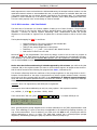
(c) Ángel M. Martin Revision 44_E Page 41 SandMath_44 Manual Pochhammer symbol: Rising and falling empires.
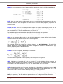
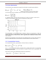
In mathematics, the Pochhammer symbol introduced by Leo August Pochhammer is the notation (x)n,
where n is a non-negative integer. Depending on the context the Pochhammer symbol may represent
either the rising factorial or the falling factorial as defined below. Care needs to be taken to check
which interpretation is being used in any particular article.
(n)
is used for the rising factorial (sometimes called the "Pochhammer function",
The symbol x
"Pochhammer polynomial", "ascending factorial", "rising sequential product" or "upper factorial"):
The symbol (x)n is used to represent the falling factorial (sometimes called the "descending
factorial",[2] "falling sequential product", "lower factorial"):
These conventions are used in combinatory. However in the theory of special functions (in particular
the hypergeometric function) the Pochhammer symbol (x)n is used to represent the rising factorial.
Extreme caution is therefore needed in interpreting the meanings of both notations !
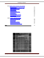
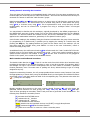
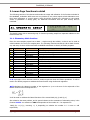
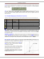
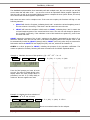
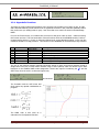
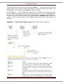
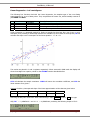
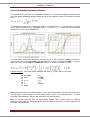
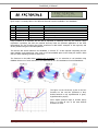
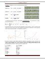
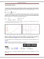
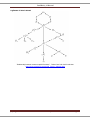
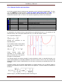
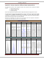
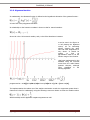
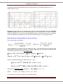
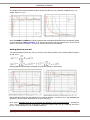
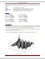
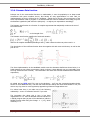
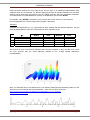
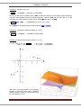
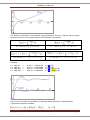
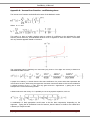
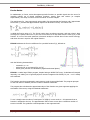
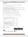
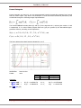
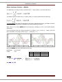
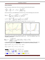
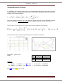
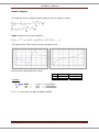
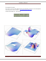
The figures below show the rising (left) and falling factorials for n={0,1,2,3,4}, and -2<x<2
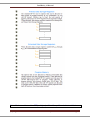
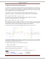
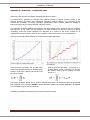
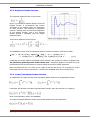
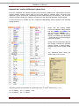
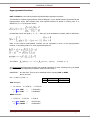
Function POCH calculates the rising factorial. It expects n and x to be in the Y and X registers
respectively (i.e. the usual convention). For large values of n the execution time may be very long – you
can hit any key to stop the execution at any time.
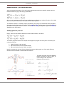
The falling factorial is related to it (a.k.a. Pochhammer symbol) by :
(n)
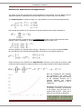
The usual factorial n! Is related to the rising factorial by:
n!=1
Whereas for the falling factorial the expression is:
n ! = (n)n
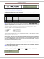
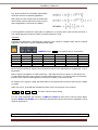
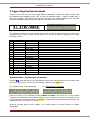
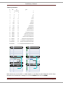
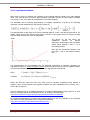
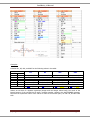
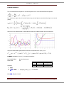
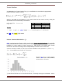
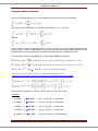
Examples: Calculate the rising factorial for n=7, x=4, and the falling factorial for n=7, x=7
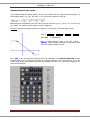
7, ENTER^, 4, XEQ “POCH”
7, ENTER^, 7, CHS, XEQ “POCH”, 7, XEQ “CHSYX”
-> 604.800,0000,
-> 5.040,000000
(c) Ángel M. Martin Revision 44_E Page 42 SandMath_44 Manual Multifactorial, Superfactorial and Hyperfactorial.
This section covers the main extensions and generalizations of the factorial. There are different ways to
expand the definition, depending on the actual sequences of numbers used in the calculation.
The double factorial of a positive integer n is a generalization of the usual factorial n!, defined by:
Even though the formulas for the odd and even double factorials can be easily combined into:
The double factorial is a special case of the multifactorial, which uses the same formula but with
different “steps”: subtracting “k” (instead of “2”) from the original number, thus:
where the products run through positive integers. Obviously for k=1 we have the standard FACT.
(k)
One can define the k-th factorial, denoted by n! recursively for non-negative integers as:
Another extension to the factorial is the Superfactorial. It doesn’t use any step-size as variant, rather
it follows a similar formula but using the factorial of the numbers instead of the numbers themselves:
Both the multifactorial and (specially)
the superfactorial will exceed the
calculator numeric range rather quickly,
so the SandMath functions use a
separate
mantissa
and
exponent
approach, using registers X and Y
respectively.
Nevertheless the functions will put up a
consolidated (combined) representation
in the display, using the letter “E” to
separate both amounts. Make sure to
adjust the FIX settings as approriate:
(c) Ángel M. Martin Revision 44_E Page 43 SandMath_44 Manual Examples:
Calculate the multi- and superfactorials given below:
2345 !! !! !!
type: 6, ENTER^, XEQ “MFCT”
->
1234 !! !! !
type: 5, ENTER^, XEQ “MFCT”
->
Sf(41)
type: 41, ΣFL$ "SFCT"
->
Sf(100)
type: 100, ΣFL$ "SFCT"
->
To complete this trinity of factorials – Occasionally the hyperfactorial of n is considered. It is written
as H(n) and defined by:
The figures below show a plot for both the hyperfactorial and its logarithm – itself a convenient scale
change very useful to avoid numeric range problems. Note that they’re extended to all real arguments,
and not only the natural numbers – also called the “K-function”.
See below a couple of simple FOCAL program to calculate the hyperfactorial (which runs beyond the
numeric range dramatically soon!) and its logarithm written by JM Baillard. Understandably slow and
limited as these programs are, you can visit his web site for a comprehensive treatment using
dedicated MCODE functions for the many different possible cases.
01
02
03
04
05
06
07
08
09
10
LBL "HFCT"
1
LBL 01
RCL Y
ENTER^
Y^X
*
DSE Y
GTO 01
END
01
02
03
04
05
06
07
08
09
10
11
LBL "LOGHF"
0
LBL 01
RCL Y
ENTER^
LOG
*
+
DSE Y
GTO 01
END
(c) Ángel M. Martin Revision 44_E Page 44 SandMath_44 Manual Logarithm Multi-Factorial.
The product of all odd integers up to some odd positive integer n is often called the double factorial of
n (even though it only involves about half the factors of the ordinary factorial, and its value is therefore
closer to the square root of the factorial). It is denoted by n!!. For an odd positive integer n = 2k - 1, k
≥ 1, it is
A common related notation is to use multiple exclamation points to denote a multifactorial, the product
of integers in steps of two (n!!), three (n!!!), or more. The double factorial is the most commonly used
variant, but one can similarly define the triple factorial (n!!!) and so on. One can define the k-th
factorial, denoted by n!(k), recursively for non-negative integers as:
The figures below show the plots for X!! (right), a comparison with log(abs(gamma)) (red)
versus log(abs(doublegamma)) (green). – left.
Using the Logarithm is helpful to deal with large arguments, as these functions go beyond the
calculator numeric range very quickly. Also ran out of space in the module to have more than one
function on this subject, thus LGMF was chosen given its more general-purpose character.
The implementation is thru an all-MCODE function, yet execution times may be large depending on the
arguments.
LGMF may also be used to compute factorials, use n=1 and then E^X on the result. Obviously the
accuracy won’t be the greatest, but it’s a reasonable compromise
Examples:
2 ENTER^ , 100
XEQ "LGMF"
999 ENTER^,
123456 XEQ "LGMF"
Stack
Y
X
Input
n
x
Output
/
LGMF(x)
-> Log ( 100 !! ) = 79.53457468
-> Log ( 123456 ! ..... ! ) = 578.0564932
And now lets move to something completely unrelated: Fourier Series representation of a given
function, f(x).
(c) Ángel M. Martin Revision 44_E Page 45 SandMath_44 Manual Appendix 5.- Primorials – a primordial view.
Welcome to the intersection between factorials and prime numbers...
In number theory primorial is a function from natural numbers to natural numbers similar to the
factorial function, but rather than multiplying successive positive integers, only successive prime
numbers are multiplied. The name "primorial", attributed to Harvey Dubner, draws an analogy to
primes the same way the name "factorial" relates to factors.
There are two conflicting definitions that differ in the interpretation of the argument: the first interprets
the argument as an index into the sequence of prime numbers (so that the function is strictly
increasing), while the second interprets the argument as a bound on the prime numbers to be
multiplied (so that the function value at any composite number is the same as at its predecessor).
The figures below plot both definitions, comparing their shape and slopes:-
Prime primorial (left plot): For the nth prime
number pn the primorial pn# is defined as the
product of the first n primes (where pk is the
kth prime number):
Natural primorial (right plot): In general, for a
positive integer n such a primorial n# can also
be defined, namely as the product of those
primes ≤ n.
The FOCAL programs below can be used to calculate both flavors of primorials. Note the primordial
(pun intended) role of function PRIME?, which effectively makes this a simple application as opposed
to a full-fledge program from the scratch.
Examples: Calculate both primorials for the first 20 natural numbers.
(c) Ángel M. Martin Revision 44_E Page 46 SandMath_44 Manual Table of primorials
n
n#
pn#
pn
0
1 no prime
1
1
1
2
2
2
2
3
6
3
6
5
30
4
6
7
210
5
30
11
2310
6
30
13
30030
7
210
17
510510
8
210
19
9699690
9
210
23
223092870
10
210
29
6469693230
11
2310
31
200560490130
12
2310
37
7420738134810
13
30030
41
304250263527210
14
30030
43
13082761331670030
15
30030
47
614889782588491410
16
30030
53
32589158477190044730
17 510510
59
1922760350154212639070
18 510510
61
117288381359406970983270
19 9699690
67
7858321551080267055879090
20 9699690
71 557940830126698960967415390
01
02
03
04
05
06
07
08
09
10
11
12
13
14
15
16
17
18
19
LBL "NPRML"
ABS
INT
E
X>Y?
RTN
X<>Y
LBL 00
PRIME?
GTO 01
X<> L
GTO 03
LBL 01
ST* Y
LBL 03
DSE X
GTO 00
X<>Y
RTN
01
02
03
04
05
06
07
08
09
10
11
12
13
14
15
16
17
18
19
LBL "PPRML"
ABS
INT
E
X>Y?
RTN
STO Z
LBL 00
INCX
PRIME?
GTO 01
X<> L
GTO 00
LBL 01
ST* Z
DSE Y
GTO 00
RCL Z
END
Both routines only use the stack – no data registers or user flags are used. Clearly the numeric range
will again be the weakest link, reaching it for n=54 for PPRML and n=251 for NPRML.
(c) Ángel M. Martin Revision 44_E Page 47 SandMath_44 Manual A glimpse of what’s ahead:
“Relationship between common special functions”. Taken from John Cook’s web site:
http://www.johndcook.com/special_function_diagram.html
(c) Ángel M. Martin Revision 44_E Page 48 SandMath_44 Manual <<()'(,%6%,-4(.
A word about the approach. The Hyper-Geometric Function as a generic function generator
(or “the case of the chameleon function in disguise”).
Special functions are particular mathematical functions which have more or less established names and
notations due to their importance in mathematical analysis, functional analysis, physics, or other
applications, frequently as solutions to differential equations. There is no general formal definition, but
the list of mathematical functions contains functions which are commonly accepted as special. Some
elementary functions are also considered as special functions.
The implementations described in this manual do nothing but scratching the surface (or more
appropriately, “gingerly touching it”) of the Special Functions field, where one can easily spend several
life-times and still be just half-way through.
Implementing multiple special functions in a 41 ROM is clearly challenged by the available space in
ROM, the internal accuracy and the speed of the CPU. It is therefore understandable that more
commonality and re-usable components identified will make it more self-contained and powerful,
overcoming some of the inherent design limitations.
The Generalized Hyper-geometric function is one of those rare instances that works in our favor, as
many of the special functions can be expressed as minor variations of the general case. Indeed there
are no less than 20 functions implemented as short FOCAL programs, really direct applications of the
general case - saving tons of space and contributing to the general consistency and common approach
in the SandMath.
We have Jean-Marc Baillard to thank for writing the original HGF+, the Generalized Hyper-geometric
function - real cornerstone of the next two sections. The SandMath has an enhanced MCODE
implementation that optimizes speed and accuracy thanks again to internal usage of 13-digit OS
routines. The reuse made of it more than pays off for its lengthy code.
A few examples will illustrate this:-
Naturally this is not the case for any special function, and even it there’s such an expression it may be
more appropriate to use the direct definition instead – or an alternative one – for the implementation.
This is the case of the Bessel functions, which use the series definition in the SandMath; the Gamma
function using the Lanczos formula, etc.
With that said, let’s delve into the individual functions comprising the High-Level Math group. First off
come those more frequently used so that they have gained their place in the ROM’s main FAT. Looking
at the authorship you’ll see the tight collaboration between JM and the author, as stated in the opening
statements of this manual.
(c) Ángel M. Martin Revision 44_E Page 49 SandMath_44 Manual 3.3.1. Gamma function and associates.
Let’s further separate these by logical groups, depending on their similarities and applicability. The first
one is the GAMMA and related functions: 1/GM, PSI, PSIN, LNGM, ICGM, BETA, and ICBT – all of
them a Quantum leap from the previous functions described in the manual, both in terms of the
mathematical definition and as it refers to the required programming resources and techniques.
[ΣF]
[ΣF]
[ΣF]
[ΣF]
[ΣF]
[ΣF]
[ΣF]
[ΣF]
Function
1/GMF
BETA
GAMMA
ICBT
ICGM
LNGM
PSI
PSIN
Author
JM Baillard
Ángel Martin
Ángel Martin
JM Baillard
JM Baillard
Ángel Martin
Ángel Martin
JM Baillard
Description
Reciprocal Gamma (Continuous fractions)
Euler’s Beta function
Euler’s Gamma function (Lanczos)
Incomplete Beta function
Incomplete Gamma function
Logarithm Gamma function
Digamma (Psi) function
Polygamma function
In mathematics, the Gamma function (represented by the capital Greek letter Γ) is an extension of the
factorial function, with its argument shifted down by 1, to real and complex numbers.
If n is a positive integer, then
showing the connection
factorial function.
to
the
For a complex number z with positive
real part, the Gamma function is
defined by
Things
become
much
more
interesting in the negative semiplane, as can be seen in the plot on
the right for real arguments.
The Gamma function has become standard in pocket calculators, either as extended factorials or as
proper gamma definition. It’s already available in the HP-11C and of course on the 15C, and that has
continued to today’s models. Implementing it isn’t the issue, but achieving a reasonable accuracy is the
challenge.
A popular method uses the Stirling approximation to compute Gamma. This is relatively simple to
program, but its precision suffers for small values of the argument. A version suitable for calculators is
as follows:
Valid for Re(z)>0, and with reasonable precision when Re(z)>8.
(c) Ángel M. Martin Revision 44_E Page 50 SandMath_44 Manual For smaller values than that it’s possible to use the recurrence functional equation, taking it to the
“safe” region and back-calculating the result with the appropriate adjusting factor:
Incidentally, this method can be used for any approximation method, not only for Stirling’s.
The method used on the SandMath is the Lanczos approximation, which lends itself better to its
implementation and can be adjusted to have better precision with careful selection of the number of
coefficients used. For complex numbers on the positive semi-plane [Re(z)>0], the formula used is as
follows:
q0 =
q1 =
q2 =
q3 =
q4 =
q5 =
q6 =
75122.6331530
80916.6278952
36308.2951477
8687.24529705
1168.92649479
83.8676043424
2.5066282
Although the formula as stated here is only valid for arguments in the right complex half-plane, it can
be extended to the entire complex plane by the reflection formula,
An excellent reference source is found under http://www.rskey.org/gamma.htm, written by Viktor T.
Toth.
Let’s mention that this method yields good enough a precision that doesn’t require using the functional
equation to adjust it for small values of the argument. The obvious advantage is that without the
required program loop, the execution time is shorter and constant for any input. This becomes of
extreme importance when Gamma is used as a subroutine of more complex cases, like the Bessel J and
I functions – where the cumulative additional time is very noticeable.
(c) Ángel M. Martin Revision 44_E Page 51 SandMath_44 Manual Appendix 6.- Accuracy comparison of different Gamma implementations.
The tables below provide a clear comparison between three methods used to calculate the Gamma
function:
1. Lanczos formula, with k=6
2. Continuous fractions, and
3. Windschitl (Stirling).
Each of them implemented using both standard 10-digit and enhanced 13-digit precision routines.
The results clearly show that the best implementation is Lanczos, and that the 13-digit routines provide
a second order of magnitude improvement to the accuracy, or in other words: that it cannot
compensate for the deficiencies of the used method. We’re lucky in that the more accurate method is
faster that the second best, albeit not as fast as Stirling’s.
Obviously the extrapolation from integer case to the general case for the argument is assumed to
follow the same trend, albeit not shown in the summary tables.
Standard 10-digit Implementation
Reference
(x-1) !
Lanczos (k=6)
Continuous Fractions
Windschitl (Stirling)
x
Result
error
Result
Result
err
1
1
1,000000001
1E-09
1,000000001
1
2
1
0
1,000000001
1E-09
1,000000012
1,2E-08
1E-09
1,000000012
1,2E-08
2
3
2
0
2,000000001
5E-10
2,000000024
1,2E-08
6
4
5,999999999
-1,66667E-10
6,000000002
3,33333E-10
6,000000071
1,18333E-08
error
24
5
24,00000001
4,16667E-10
24
0
24,00000028
1,16667E-08
120
6
120
0
120
0
120,0000014
1,16667E-08
720
7
720,0000008
1,11111E-09
720,0000001
1,38889E-10
720,0000087
1,20833E-08
5040
8
5040,000002
3,96825E-10
5040
0
5040,00006
1,19048E-08
40320
9
40320,00003
7,44048E-10
40319,99999
-2,4802E-10
40320,00048
1,19048E-08
362880
10 362880,0002
5,51146E-10
362879,9998
-5,5115E-10
362879,9988
-3,30688E-09
3628800
11 3628800,001
2,75573E-10
3628800,018
4,96032E-09
3628800,05
1,37787E-08
39916800
12 39916799,99
-2,50521E-10
39916800,01
2,50521E-10
39916800,9
2,25469E-08
479,001,600
13 479001599,5
-1,04384E-09
479001598,3
-3,549E-09
479001580,2
-4,1336E-08
4,81771E-10
6227020798
-3,2118E-10
6227020957
2,52127E-08
6,227,020,800 14
6227020803
Enhanced 13-digit Implementation
Reference
Lanczos (k=6)
Continuous Fractions
Result
Windschitl (Stirling)
(x-1) !
x
Result
error
error
Result
error
1
1
1
0
1
2
1
0
1
0
1
0
1,000000001
1E-09
1
0
2
3
2
0
2
0
1.999999999
-5E-10
6
4
6
0
6.000000004
6,66667E-10
5.999999997
-5E-10
24
5
24
0
24
0
23.99999999
-4,16667E-10
120
6
120
0
120
0
120,0000014
1,16667E-08
720
7
720
0
720
0
719.9999996
-5,55556E-10
5040
8
5040
0
5039,9999990
-1,9841E-10
5,039.999998
-3,96825E-10
40320
9
40320
0
40,320.00001
2,48016E-10
40,319.99998
-4,96032E-10
362880
10
362880
0
362880
0
362,880
0
3628800
11
3628800
0
3628800
0
3,628,800
0
39916800
12
39916800
0
39916800
0
39,916,799.99
-2,50521E-10
479,001,600
13
479001600
0
479001600
0
479,001,599.8
-4,17535E-10
6,227,020,800 14
6227020800
0
6227020800
0
6,227,020,800
0
(c) Ángel M. Martin Revision 44_E Page 52 SandMath_44 Manual 3.3.2. Reciprocal Gamma function.
The reciprocal Gamma function is the function
where Γ(z) denotes the Gamma function. Since the
Gamma function is meromorphic and nonzero
everywhere in the complex plane, its reciprocal is
an entire function. The reciprocal is sometimes
used as a starting point for numerical computation
of the Gamma function, and a few software
libraries provide it separately from the regular
Gamma function.
Taylor series expansion around 0 gives
The SandMath however uses the expression based in continuous fractions, according to which:
Γ(x) = [x^(x-1/2)] sqrt(2π) exp [ -x + (1/12)/(x +
+ (1/30)/(x + (53/210)/(x +(195/371)/(x + ...
))))]
Comparing the results obtained by GAMMA (using Lanczos) and continuous fractions it appears that
the precision is generally better in the Lanczos case – which also happens to be faster due to its
polynomial-like form and the absence of loops to adjust the result for smaller arguments.
Note the special case for x=0, which is not a pole for this function but it is a singularity for all the
others that used the common subroutines – therefore the dedicated check in the routine listing.
3.3.3. (Lower) Incomplete Gamma function.
In mathematics, the upper and the lower incomplete gamma functions are respectively as follow:
Connection with Kummer's confluent hypergeometric function, when the real part of z is positive,
which is the expression used in the SandMath.
The Upper incomplete Gamma function can be easily obtained from the relationship:
(c) Ángel M. Martin Revision 44_E Page 53 SandMath_44 Manual 3.3.4. Log Gamma function.
Many times is easier to calculate the Logarithm of the Gamma function instead of the main Gamma
value. This could be due to numeric range problems (remember that the 41 won’t support numbers
over E100), or due to the poles and singularities of the main definition.
The SandMath uses the Stirling approximation to compute LogGamma, as given by the following
expression (directly obtained from the formula in page 27):
This approximation is also good to more than 8 decimal digits for z with a real part greater than 8. For
smaller values we’ll use the functional equation to extend it to the region where it’s accurate enough
and then back-calculate the result as appropriate.
The picture on the left shows the
LogGamma
function
for
positive
arguments. Interestingly it has a negative
results region between 1 and 2 – so it
isn’t always positive.
Note also the asymptotic behavior near
the origin – due to the Gamma function
pole.
The implementation on the SandMath uses the analytical continuation to calculate LogGamma for
arguments less than 9, including negative values. Obvious problems (like the poles at negative integer)
will yield DATA ERROR messages, but outside that the approximation should hold.
since:
Γ (z+n) = Γ(z) * Σ(z+i) |
it follows:
Ln Γ (z+n) = Ln Γ(z) + Ln [Σ(z+i) |
i=1,2..n
i=1,2..n]
Notice also that the same error will occur when trying to calculate LogGamma when Gamma is
negative, which occurs between even-negative numbers and their immediately lower (inferior) one –
see the plot in page 27).
See the following link for a detailed description of another implementation (using Lanczos for both
cases) to calculate Gamma and LogGamma on the 41 by Steven Thomas Smith:
http://www.hpmuseum.org/cgi-sys/cgiwrap/hpmuseum/articles.cgi?read=941
An excellent implementation of Gamma and related functions for the 41 is available on the following
link, written by Jean-Marc Baillard (very complete and detailed):
http://www.hpmuseum.org/software/41/41gamdgm.htm
(c) Ángel M. Martin Revision 44_E Page 54 SandMath_44 Manual 3.3.5. Digamma function.
In mathematics, the digamma function is defined as the logarithmic derivative of the gamma function:
It is the first of the polygamma functions.
Its relationship to the harmonic numbers is shown in that for natural numbers:
where Hn is the n'th harmonic number, and γ is the Euler-Mascheroni constant.
As can be seen in the figure on
the left plotting the digamma
function, it’s an interesting
behavior showing the same
poles and other singularities to
worry about. It should be
possible
to
find
an
approximation valid for all the
definition range of the function.
It has been implemented on the
SandMath using the formulas
derived from the called Gauss
digamma theorem, although
further
simplified
in
the
following algorithm:
programmed as: u^2{[(u^2/20-1/21)u^2 + 1/10]u^2 –1}/12 – [Ln u + u/2],
The implementation also makes use of the analytic continuation to take it to arguments greater than 9
(same as it’s done for LogGamma), using the following recurrence relation to relate it to smaller values:
Which naturally can be applied for negative arguments as well.
(c) Ángel M. Martin Revision 44_E Page 55 SandMath_44 Manual 3.3.6. Euler’s Beta function.
The beta function, also called the Euler integral of the first kind, is a special function defined by
The beta function was studied by Euler and Legendre and was given its name by Jacques Binet.
The most common way to formulate it refers to its relation to the Gamma function, as follows:
As a graphical example, the picture below shows B(X,0.5) for values of x between –4 and 4. As it’s
expected, the same Gamma problem points are inherited by the Beta function.
The implementation on the SandMath makes no attempt to discover new approaches or utilize any
numeric equivalence: it simple applies the definition formula using the Gamma subroutine. Obvious
disadvantages include the reduced numeric range – aggravated by the multiplication of gamma values
in the numerator.
Execution time corresponds to three times that of the Gamma function, plus the small overhead to
perform the Alpha Data checks and the arithmetic operations between the three gamma values.
3.3.7. Incomplete Beta Function.
The incomplete beta function, a generalization of the beta function, is defined as:
For x = 1, the incomplete beta function coincides with the complete beta function. The relationship
between the two functions is like that between the gamma function and its generalization the
incomplete gamma function.
And it’s given in terms of the Hypergeometric function the expression by:
(c) Ángel M. Martin Revision 44_E Page 56 SandMath_44 Manual 3.3.8. Bessel functions and Modified.
The next logical group would be the Bessel functions – with special guests Riemann’s ZETA and
Lambert’s W (both branches).
[ΣF]
[ΣF]
[ΣF]
[ΣF]
[ΣF]
[ΣF]
[ΣF]
[ΣF]
Function
IBS
JBS
KBS
SIBS
SJBS
SYBS
WL0
WL1
YBS
ZETA
ZETAX
Author
Ángel Martin
Ángel Martin
Ángel Martin
Ángel Martin
Ángel Martin
Ángel Martin
Ángel Martin
Ángel Martin
Ángel Martin
Ángel Martin
JM Baillard
Description
Bessel I(n,x) of the first kind
Bessel J(n,x) of the first kind
Bessel K(n,x) of the second kind
Spherical Bessel i(n,x)
Spherical Bessel j(n,x)
Spherical Bessel y(n,x)
Lambert’s W - main branch
Lambert’s W – secondary branch
Bessel Y(n,x) of the second kind
Riemann’s Zeta – direct method
Riemann’s Zeta – Borwein algorithm
The SandMath Module includes a set of functions written with the harmonic analysis in mind,
specifically to facilitate the calculation of the Bessel functions in their more general sense: for any real
number for order and argument.
Bessel functions of the First kind – I(n,x) and J(n,x)
The formulae used are as follows:
Where Γ denotes the Gamma function.
These expressions are valid for any real number as order, although there are issues for negative
integers due to the singularities in the poles of the gamma function - as there’s always a term for which
(m+n+1) equals zero or negative integers, all of them being problematic.
To avoid this, we use the following expression for negative integer orders:
Whilst:
I-α(x) = Iα(x),
for every real number order.
This definition is also valid for negative values for X, as there’s no singularity for any x value.
The SandMath implementation uses a recurrence formula instead of the one shown above. It has the
clear advantage of not having to calculate Gamma for each term in the sum, contributing to a much
faster and robust algorithm.
The iterative relationships are as follows:
J(n,x) = Σ{U(k)|k=1,2…} * (x/2)n / Γ(n+1),
U(k) = - U(k-1) * (x/2)^2 / k(k+n),
where:
with U(0) = 1.
(c) Ángel M. Martin Revision 44_E Page 57 SandMath_44 Manual The graphics below plot the Bessel functions of the first kind, Jα(x), and their modified, Iα(x), for
integer orders α=0,1,2,...
Note that for large values of the argument, the order or both these algorithms will return incorrect
results for J(n,x). This is due to the alternating character of the series, which fools the convergence
criteria at premature times and fouls the intermediate results. Unfortunately there isn’t an absolute
criteria for validity, but a practical rule of thumb is to doubt the result if (n+x) it greater than 20.
Bessel functions of the Second kind – K(n,x) and Y(n,x)
The formulae used are as follows:
These expressions are valid for any real number as order – with the same issues as the first kind
functions above when the order is integer. To avoid the singularities and to reduce the calculation time,
the following expressions are used for integer orders:
π Yn(x) = 2[γ + Ln x/2] Jn(x) – Σ{(-1)k fk(n,x)} – Σ{gk(n,x)}
2 Kn(x) = (-1)n+1 2 [γ + Ln x/2] In(x) + (-1)n Σ{ fk(n,x)} + Σ{(-1)k gk(n,x)}
where γ is the Euler–Mascheroni constant (0.5772...), and:
gk(n,x) = (x/2)2k-n (n-k-1)! / k! ; k=0,1,2,…(n-1)
fk(n,x) = (x/2)2k+n [H(k) + H(n+k)] / [k! (n+k)!] ; k=0,1,2,…..
and H(n) is the harmonic number, defined as:
Where:
H(n) = Σ(1/k) | k = 1,2,.. n
Y–n(x) = (-1)nY n (x), and K–n (x) = Kn(x)
(*) note that for x<0, Y(n,x) and K(n,x) are complex numbers.
(c) Ángel M. Martin Revision 44_E Page 58 SandMath_44 Manual The graphics below plot the Bessel functions of the second kind, Yα(x), and their modified, Kα(x), for
integer orders α=0,1,2,...
Note that KNBS and YNBS are FOCAL programs that use dedicated MCODE functions specially written
for the calculations (#BS and #BS2). Their entries are located in the sub-functions FAT, thus won’t be
shown in the main CAT listings – in case you wonder about their whereabouts.
Getting Spherical, are we?
The spherical Bessel functions jn and yn, and are (very closely) related to the ordinary Bessel functions
Jn and Yn by:
Which graphical representation (naturally very JBS-ish looking) is show below:
Notice that there really isn’t any Spherical i(n,x) properly defined – but there’s one in the SandMath just
the same, using the same relationship as for j(n.x) and y(n,x).
Once again, remember than as (n+x) increases the accuracy of the results decreases – specially for
J(n,x), Y(n,x) and the spherical counterparts, where the returned value can be completely incorrect if
(n+x) > 20 (a practical rule, not an absolute criterion).
(c) Ángel M. Martin Revision 44_E Page 59 SandMath_44 Manual Programming Remarks.
The basic algorithms use the summation definition of the functions, calculating the successive values of
the sum until there’s convergence for the maximum precision (10 decimal places on the display).
Therefore the execution time can take a little long – a fact that becomes a non-issue on the CL. Or
when using 41-emulator programs, like V41, setting the turbo mode on.
There are different algorithms depending on whether the order is integer or not. This speeds up the
calculations and avoids running into singularities (as mentioned before).
Note that for integer indexes the gamma function changes to a factorial calculation, which benefits
from faster execution on the calculator. Non-integer orders utilize the special MCODE function,
GAMMA, with shorter execution times than equivalent FOCAL programs – but still longer than FACT
when integers.
Besides that, for integer orders the execution time is further reduced by calculating simultaneously
the two infinite sums involved in the first kind and the second kind terms. This assumes that the
convergence occurs at comparable number of terms, which fortunately is the case - given their relative
fast convergence.
Note that in order to obtain similar expressions for both Yn and Kn – and so getting simpler program
code - we can re-write Kn as follows:
(-1)n+1
2 Kn(x) = 2 [γ
+ Ln x/2] In(x) – Σ{ fk(n,x)} – (-1)n Σ{(-1)k gk(n,x)}
Dedicated MCODE Functions.
To further decrease the execution time of the programs, two dedicated functions have been written,
implemented as MCODE routines as follows:
Function
Flag 00 Clear
Flag 00 Set
--------------------------------------------------------------------------------Σ Uk(n,x), |k=0,1,2 where Uk =- Uk-1 * (x/2)^2 / k(k+n)
#BS
#BS2
Σ{fk(n,x)} |k=0,1,2… or:
Σ{gk(n,x)} |k=0,1,…(n-1)
The first function #BS is used equally in the calculation of the first kind and the second kind of noninteger orders.
Function
JBS
IBS
YBS
KBS
Integer
Non-integer
#BS
2x #BS2
#BS
As it was said before, the summation will continue until the contribution of the newer term is negligible
to the total sum value. All calculations are done using the full 13-digit precision of the calculator. No
rounding is made until the final comparison, which is done on 10-digit values.
From the definition above it’s clear that #BS coincides with either Jn(x) or In(x) depending on the
status of the CPU flag 9, and for positive orders. The functions JBS and IBS are just MCODE
extensions of #BS that set up the specific settings prior to invoking it, and (depending on the signs of
the orders and the arguments) possibly adjust the result after it’s completed.
(c) Ángel M. Martin Revision 44_E Page 60 SandMath_44 Manual The second function #BS2 is only used for second kind functions with integer orders. It’s a finite sum,
and not an infinite summation. Its contribution to the final result grows as the function order increases.
Its main goal was to reduce execution time as much as possible, derived from the speed gains of
MCODE versus FOCAL.
The definition of fk(n,x) is as follows:
f k(n,x) = {(x/2)2k+n / [k! (n+k)!] } [H(k) + H(n+k)] ;
k=0,1,2…
The definition of gk(n,x) is as follows:
gk(n,x) = (x/2)2k-n (n-k-1)! / k! ; k=0,1,…(n-1)
The calculation of Gamma uses the Lanczos approximation implemented in the GAMMA function of the
SandMath. Despite being reasonably fast, its execution time is noticeably longer than that of the
Factorial for integer indexes – therefore #BS2 will use FACT instead for integer orders.
The Harmonic Numbers H(n) are obtained using another SandMath function as subroutine, Σ1/N. You
see that the internals of #BS2 perform quite an involved procedure, utilizing multiple resources within
the SandMath module.
Furthermore, #BS2 is called twice within the FOCAL program to calculate KBS or YBS – once for the
first, infinite summation and a second time for the second, finite sum. The status of User Flag 00
controls the calculation made. That was done to save one FAT entry, when the limiting factor was the
maximumm nuber of functions per page (i.e. 64 functions). Now they have been pushed eveh further
off, to the secondary FAT used for the sub-functions group.
Bessel Function
Yn(x)
Kn(x)
Summed Functions by #BS2
gk(n,x)
fk(n,x)
(-1)k * gk(n,x)
(-1)k * fk(n,x)
Flag 00
Set
Clear
Set
Clear
Flag 01
Set
Clear
Note also that for this case (integer orders) there’s two infinite summations involved for the Bessel
functions of the second kind. This is done simultaneously within #BS2 when user flag 02 is set, as
both series converge in very similar conditions (i.e. with the same number of terms).
Main functions: IBS, JBS, KBS, and YBS.
The first kind pair (IBS and JBS) are 100% written in MCODE – including exception handling and
special cases. This is the only version known to the author of a full-MCODE implementation on the 41
platform, and it is however a good example of the capabilities of this machine.
No data registers are used for IBS and JBS – but both the stack and the Alpha registers are used. The
number of terms required for the convergence is stored in register N upon termination.
The second kind pair (KBS and YBS) is implemented using a FOCAL driver program for #BS and
#BS2. Notably more demanding than the previous two, their expressions require additional
calculations that exceed the reasonable MCODE capabilities.
Although they’re not normally supposed to be used outside of the Bessel program, #BS and #BS2
could be called independently. Both use the same input parameters: index in Y and half of the
argument in X. Pay close attention to the status of user flags 00 and 01 as they directly influence their
result.
(c) Ángel M. Martin Revision 44_E Page 61 SandMath_44 Manual Other functions used in the Bessel calculations, which aren’t part of the native HP-41 function set, are
as follows:
GEU
CHSYX
INT? and FRC?
E3/E+
Euler’s constant = 0,577215665
CHS repeated n times (in X register) multiplied by Y register.
Conditional based on value in X being integer or fractional
Self-explanatory: divides X by 1,000, then adds one.
Examples:
J(1,1) = 0,440050586
J(-1,-1) = 0,440050586
J(0.5,0.5) = 0,540973790
J(-0.5, 0.5) = 0,990245881
I(1,1) = 0,565159104
I(-1,-1) = -0,565159104
I(0.5,0.5) = 0,587993086
I(-0.5,0.5) = 1,272389647
Y(1,1) = -0,781212821
Y(-1,2) = 0,107032431
Y(0.5,0.5) = -0,990245881
Y(-0.5,0.5) = 0,540973790
K(1,1) = 0,601907230
K(-1,2) = 0,139865882
K(0.5,0.5) = 1,075047604
K(-0.5,0.5) = 1,075047604
Error Messages:
Note that the functions will return a “DATA ERROR” message when the solution is a complex number,
like J(-0.5, -0.5) or I(-0,5, -0.5). There’s no way around that save in some particular cases of the order.
You can always use the versions available in the 41Z Module for a full complex range.
“OUT OF RANGE”, when the calculator numeric range is exceeded. This typically occurs for large
indexes, during the power exponentiation step.
“ALPHA DATA” indicates alphabetic data in registers X or Y. May also trigger “DATA ERROR”.
(c) Ángel M. Martin Revision 44_E Page 62 SandMath_44 Manual Appendix 7.- FOCAL program used to calculate the Bessel Functions of the second kind. As you can
see it’s just a simple driver of the MCODE functions, with the additional task of orchestrating the logic
for the different cases.
Note the usage of the sub-functions from the auxiliary FAT , as well as other SandMath functions.
01
02
03
04
05
06
07
08
09
10
11
12
13
14
15
16
17
18
19
20
21
22
23
24
25
26
27
28
29
30
31
32
33
34
35
36
37
38
39
40
41
42
43
44
45
46
47
48
49
50
LBL "KBS"
SF 01
GTO 00
LBL "YBS"
CF 01
LBL 00
X=0?
RTN
2
/
STO 03
X<>Y
STO 01
INT?
GTO 02
CHS X<>Y
RAD
SPFC#
1
CHS STO 02
RCL 01
RCL 03
SPFC#
1
STO 00
FC? 01
GTO 01
RCL 01
PI
*
COS
*
LBL 01
RCL 02
+
RCL 01
PI
*
SIN
/
FS? 01
GTO 03
2
/
PI
*
CHS GTO 03
single case x=0
HALFX
x/2
s wa p thi ngs n
is it integer order?
yes, divert to section
‐n
x/2
Multi‐Function Launcher
Recurrence Sum #BS
‐J(‐n,x)
pa rti a l res ul t
n
x/2
Multi‐Function Launcher
Recurrence Sum #BS
save J(n,x) here ‐ used by Hankel
i s KBS?
yes , s ki p
n
pa rti a l res ul t
n
i s YBS?
HALFX
(c) Ángel M. Martin Revision 44_E 51
52
53
54
55
56
57
58
59
60
61
62
63
64
65
66
67
68
69
70
71
72
73
74
75
76
77
78
79
80
81
82
83
84
85
86
87
88
89
90
91
92
93
94
95
96
97
98
99
100
101
LBL 02
CF 02
X<0?
SF 02
ABS
STO 01
,
STO 00
STO 02
RDN
X=0?
GTO 06
CF 00
SPFC#
2
CHS
STO 02
RCL 01
LBL 06
RCL 03
SF 00
SPFC#
2
ST‐ 02
RCL 03
LN
GEU
+
RCL*
ST+ X(3)
ST+ 02
RCL 02
FS? 01
GTO 04
RCL 01
E
+
CHSYX
2
/
GTO 03
LBL 04
PI
/
FC? 02
GTO 03
RCL 01
CHSYX
LBL 03
STO 02
END orden,argument swapped
defa ul t ca s e
is it negative?
negative order
remember this fact!
abs(n)
res et counter
and partial sum
s ki p i f n=0
selects #B2
Σ[gk(n,x)] |k=0,1…(n‐1)
#BS2
abs(n)
x/2
selects #B1
Σ[fk(n,x)] |k=0,1,2…
#BS2
partial result
showing off ! :‐)
partial result
i s i t YBS?
yes , cut the cha s e
abs(n)
INCX
(‐1)^n+1 * result
HALFX
was negative order?
no, skip correction
abs(n)
final result
Page 63 SandMath_44 Manual 3.3.9. Riemann Zeta function.
Perhaps one of the most-studied functions in mathematics, it owes its popularity to its deep-rooted
connections with prime numbers theory. Not having an easy approximation to work with, its
implementation on the 41 will be a bit of a challenge – mainly due to the very slow convergence of the
series representation used to program it. Be assured that this numeric calculation won’t help you prove
the Riemann hypothesis (and collect the $1M prize) – so adjust your expectations accordingly.
The Riemann zeta function is a function of complex argument s that analytically continues the sum of
the infinite series
or the integral form:
The Riemann zeta function satisfies the functional equation
valid for all complex numbers s (excluding 0 and 1), which relates its values at points s and 1−s.
The plots below of the real Zeta function show the negative side with some trivial zeros, as well as the
pole at x=1.
The direct implementation in the SandMath module uses the alternative definitions shown below, in a
feeble attempt to get a faster convergence (which in theory it does although not very noticeably given
the long execution times involved). The summations are called the Dirichlet Lambda and Eta functions
respectively.
Go ahead and try ZETA with FIX 9 set in the calculator – you’ll see the successive iterations being
shown for each additional term, until the final result doesn’t change. Be aware than MCODE or not, it’ll
take a very long time for small arguments, approaching infinite as x approaches zero.
For values lower than 1 we make use of the following
relationship – a sort of “reflection formula” if you wish.
The interesting fact about this is how it has been
implemented: if x<1 then the MCODE function branches to
a FOCAL program that (as part of the calculations) calls the
MCODE function after doing the change: x = (1-x), which
obviously is >1.
(c) Ángel M. Martin Revision 44_E Page 64 SandMath_44 Manual Really the direct method isn’t very useful at all, and it’s more of an anecdotal implementation with
academic value but not practical. The Borwein algorithm provides an iterative alternative to the direct
method, with a much faster convergence even as a FOCAL program, and more comfortable treatment.
It is implemented in the SandMath as a courtesy of JM Baillard, in the function ZETAX.
For example, using ZETAX to calculate Ζ(1.001) returns the correct solution is a few seconds!
See the appendices for a FOCAL listing of the program if interested.
Examples.Complete the table below for ζ(x), using both the direct method and the Borwein algorithm. Use the
result in WolframAlfa as reference to also determine their respective errors.
x
-5
5
3
2
1,1
ζ(x) -0,0039682539682
1,036927755
1,202056903
1,6449340668482
10,58444846
Direct
-0,003968254
1,03692775
1,20205676
n/a
n/a
error
Borwein
error
8,0136E-09 -0,003968254 8,0136E-09
-4,96019E-09 1,036927755 -1,38255E-10
-1,19096E-07 1,202056903 -1,32764E-10
n/a
1,644934066 -5,15644E-10
n/a
10,58444847 4,77115E-10
We see that not only is the Borwein algorithm faster and more capable in range, but also their results
are more accurate than the direct approach; MCODE or not, 13-digit internal subroutines
notwithstanding.
Note: The following links to the MAA and the (now defunct) Zetagrid make fascinating reading on the
Zeta zeros current trends and historic perspective – make sure you don’t miss them!
http://www.maa.org/editorial/mathgames/mathgames_10_18_04.html
http://www.zetagrid.net/
(c) Ángel M. Martin Revision 44_E Page 65 SandMath_44 Manual Appendix 8.- Putting Zeta to work: Bernoulli numbers.
In mathematics, the Bernoulli numbers Bn are a sequence of rational numbers with deep connections
to number theory. The values of the first few Bernoulli numbers are
B0 = 1, B1 = ±1⁄2, B2 = 1⁄6, B3 = 0, B4 = −1⁄30, B5 = 0, B6 = 1⁄42, B7 = 0, B8 = −1⁄30.
If the convention B1=−1⁄2 is used, this sequence is also known as the first Bernoulli numbers; with the
convention B1=+1⁄2 is known as the second Bernoulli numbers. Except for this one difference, the first
and second Bernoulli numbers agree. Since Bn=0 for all odd n>1, and many formulas only involve
even-index Bernoulli numbers, some authors write Bn instead of B2n.
The Bernoulli numbers were discovered around the same time by the Swiss mathematician Jakob
Bernoulli, after whom they are named, and independently by Japanese mathematician Seki Kōwa.
Seki's discovery was posthumously published in 1712 in his work Katsuyo Sampo; Bernoulli's, also
posthumously, in his Ars Conjectandi of 1713. Ada Lovelace's note G on the analytical engine from
1842 describes an algorithm for generating Bernoulli numbers with Babbage's machine. As a result, the
Bernoulli numbers have the distinction of being the subject of the first computer program.
There are several (or rather many!) algorithms and approaches to
the calculation of Bn. In this particular example we’ll use the
expression based on the Riemann’s Zeta function, according to
which the values of the Riemann zeta function satisfy
n ζ(1 − n) = −Bn
for all integers n≥0. The expression n ζ(1 − n) for n = 0 is to be
understood as the limit of x ζ(1 − x).) when x->0.
The FOCAL program on the right is a super-short application of the
ZETA function, even if it’s used for negative arguments, Obviously
we’ve single-cased the troublesome points to avoid execution times
unreasonably long, but apart from that it’s quite generic in its
approach. It also uses a few others SandMath functions as additional
bonus.
(c) Ángel M. Martin Revision 44_E Page 66 SandMath_44 Manual 3.3.10. Lambert W function.
The last function deals with the implementation of the Lambert W function. Oddly enough its definition
is typically given as the inverse of another function, as opposed to having a direct expression. This
makes it a bit backwards-looking initially but in fact it is significantly easier to implement than the
Riemann Zeta seen before.
The Lambert W function, named after Johann Heinrich Lambert, also called the Omega function or
product log, is the inverse function of f(w) = w exp(w) where exp(w) is the natural exponential
function and w is any complex number. The function is denoted here by W.
For every complex number z:
The Lambert W function cannot be expressed in
terms of elementary functions. It is useful in
combinatory, for instance in the enumeration of
trees.
It can be used to solve various equations
involving exponentials and also occurs in the
solution of delay differential equations.
The Taylor series of W0 around 0 can be found using the Lagrange inversion theorem and is given by:
where n! is the factorial. However, this series oscillates between ever larger positive and negative
values for real z>~0.4, and so cannot be used for practical numerical computation.
The W function may be approximated using Newton's method, with successive approximations to w =
W(z) (so z = w ew) being:
The implementation in the SandMath uses this iterative method to solve for W(z) the roots of its
functional equation, given the functions argument z. An important consideration is the selection of the
initial estimations. For that the general practice is to start with Ln(x) as lower limit, and 1+Ln(x) as
upper value.
Another aspect of the W function is the existence of two branches. The second branch is defined for
arguments between –1/e and 0, with function values between –1 and –infinite.
The “lower” branch is also available in the SandMath as the function WL1. In fact the MCODE
algorithm is the same one, with just different initial estimations depending on the branch to calculate!.
(c) Ángel M. Martin Revision 44_E Page 67 SandMath_44 Manual Example 1: calculate W for x=5
5, WL0 -> “RUNNING…”, followed by 1,326724665
We can use the inverse Lambert function AWL to check the accuracy of the results, simply executing it
after WL0 and comparing with the original argument. Note the AWL will be seen later on, in the
Secondary FAT (Sub-functions) group. This it requires ΣFL$ to call it, not XEQ.
5, WL0 , ΣFL$ “AWL” -> 4,999999998; an error of err= 4 E-10
where ΣFL$ can be called using the main launcher: [ΣFL], [ALPHA]
Example 2.- calculate the Omega constant, ω = W(1)
1, WL0 => “RUNNING…” , followed by 0,567143290
Example 3: Calculate both branches of W for x=-1/2e
1, E^X, CHS, ST+ X, 1/X, WL0
LASTX, XEQ “WL1“
-> W0 (-1/2e) = -0,231960953
-> W-1(-1/2e) = -2,678346990
And here’s a 3D representation of the complex
Lambert to end this section with a graphical
splash. Enough to make you want to start using
your 41Z Module, isn’t it?
(c) Ángel M. Martin Revision 44_E Page 68 SandMath_44 Manual 3.4. Remaining Special Functions in the Main FAT.
The third and last chapter of the Special functions in the main FAT comprises other Hyper-geometric
derived functions, plus a couple of notable exceptions not easy to associate: FFOURN and LINX
[ΣF]
[ΣF]
[RF]
[ΣF]
[H]
[H]
[ΣF]
Function
CI
EI
ELIPF
ERF
FFOUR
HCI
HGF+
HSI
LINX
SI
Author
JM Baillard
JM Baillard
Ángel Martin
JM Baillard
Ángel Martin
JM Baillard
JM Baillard
JM Baillard
Ángel Martin
JM Baillard
Description
Cosine Integral
Exponential Integral
Eliptic Integral
Error Function
Fourier coefficients for (x)
Hyperbolic Cosine Integral
Generalized Hyper-geometric Function
Hyperbolic Sine Integral
Dilogarithm function
Sine Integral
Notable examples of “multi-purposed function” are also the Carlson Integrals, themselves a generator
for several other functions like the Elliptic Integrals. More about this in the corresponding paragraphs
later on.
Exponential Integral and associates.
The first sub-section covers the Exponential, Logarithmic, Trigonometric and Hyperbolic integrals.
They’re all calculated using their expressions using the Generalized Hyper-geometric function, in a clear
demonstration of the usefulness or the adopted approach.
For real nonzero values of x, the exponential integral Ei(x) is defined as:
Integrating the Taylor series for exp(t) and extracting the logarithmic singularity, we can derive the
following series representation for real values:
where we substitute the series by its Hyper-Geometric representation:
Σ{ x^k / k k!} = x * 2F2( 1, 1 ; 2, 2; x )
The logarithmic integral has an integral representation defined for all positive real numbers by the
definite integral:
The function li(x) is related to the exponential integral Ei(x) via the equation:
which is the one used to program it in the SandMath module.
(c) Ángel M. Martin Revision 44_E Page 69 SandMath_44 Manual The different trigonometric and hyperbolic integral definitions and their relations with the HyperGeometric funcion (for the relevant integral in the definition) are as follows:
x * 1F2(1/2; 3/2, 3/2; -x2/4 )
x * 1F2( 1/2 ; 3/2 , 3/2 ; x2/4 )
-(x2/4) 2F3( 1, 1 ; 2, 2, 3/2 ; -x2/4 )
(x2/4) 2F3( 1, 1 ; 2, 2, 3/2 ; x2/4 )
Examples:
1.4
1.4
1.4
1.4
XEQ
XEQ
XEQ
XEQ
"SI"
"CI"
"SHI"
"CHI"
->
->
->
->
Si(1.4) = 1.256226733
Ci(1.4) = 0.462006585
Shi(1.4) = 1.561713390
Chi(1.4) = 1.445494076
- or: [ΣF], [Z]
- or: [ΣF], [V]
- or: [ΣF], [SHIFT], [Z]
- or: [ΣF], [SHIFT], [V]
Even if it’s not covered by the SandMath, the following relation between the Exponential and
Trigonometric Integrals is available:
(c) Ángel M. Martin Revision 44_E Page 70 SandMath_44 Manual Errare humanum est.
In mathematics, the error function (also called the Gauss error function) is a special function (nonelementary) of sigmoid shape which occurs in probability, statistics and partial differential equations. Its
definition and the expression based on the Hyper-geometric function (via ascending series) are given in
the table below:
erf x = (2x/π1/2) exp(-x2) 1F1( 1, 3/2 ; x2 )
The complementary error function, denoted erfc, is defined as :
erfc = 1 – erf (x)
Both functions are shown below for an overview.
The unsung hero: HGF+
If we’re to believe that behind a great man there is often an even greater woman, then the greatest
idea behind all these functions is the implementation of the Generalized Hyper-geometric function. A
general-purpose definition requires the use of data registers for the parameters (a1... am) and (b1, ...
bn) , and expects the argument x in the X register, and the number of parameters m and n is stored in
Z and Y, for the generic expression:
mFp(a1,a2,....,am ;
b1,b2,....,bp ; x ) =
=
•
•
•
•
•
•
Σk=0,1,2,..... [(a1)k(a2)k.....(am)k] / [(b1)k(b2)k.....(bp)k] . xk/k!
If m = p = 0 , HGF+ returns exp(x)
The program doesn't check if the series are convergent or not.
Even when they are convergent, execution time may be prohibitive: press any key to stop
Stack register T is saved and x is saved in L-register.
R00 is unused.
The alpha "register" is cleared.
The original HGF+ was written by Jean-Marc Baillard. Only small changes have been made to the
version in the SandMath, optimizing the code and checking for ALPHA DATA in all registers used, as
well as for the argument x.
(c) Ángel M. Martin Revision 44_E Page 71 SandMath_44 Manual Appendix 9.- Inverse Error Function.- coefficients galore…
The inverse error function can be defined in terms of the Maclaurin series
Where c0 = 1 and
This really is a bear to handle, requiring quite a number of coefficients to be calculated for good
accuracy result. Moreover, that calculation involves a lot of registers to store the values – since there
isn’t any iterative approach based on recursion.
The expression below is definitely too inaccurate (only three or four digits are correct) to deserve a
dedicated MCODE function:
A paper from 1968 by A. Strecok lists the first 200 coefficients of a power series that represents the
inverse error function. While using this approach it became clear that at least 30 of them are needed for
a 10-digit accuracy for 0< x < 0,85. This only gets worse as x approaches 1, getting into a clear
example of the “law of diminishing results”.
A better method for the vicinity of 1 is probably to use an asymptotic expansion, such as:
A combination of both approaches would seem to be the best compromise, depending on the
argument. . Typing the 30 coefficients is not fun however, thus the best is no doubt to use a data file in
X-Memory to keep them safe.
(c) Ángel M. Martin Revision 44_E Page 72 SandMath_44 Manual How many logarithms, say again?
LINX calculates the polylogarithm function, (also known as Jonquière's function) a special function
defined by the infinite sum, or power series:
Only for special values of the order s does the polylogarithm reduce to an elementary function such as
the logarithm function. The above definition is valid for all complex orders s and for all complex
arguments z with |z| < 1; it can be extended to |z| ≥ 1 by the process of analytic continuation.
For particular cases, the polylogarithm may be expressed in terms of other functions (see below).
Particular values for the polylogarithm may thus also be found as particular values of these other
functions. For integer values of the polylogarithm order, the following explicit expressions are known:
The SandMath implementation is a direct series summation, adding terms until their contribution to the
sum is negligible. Convergence is very slow, especially for small arguments. Its usage expects n to be
in register Y and x in register X. The result is saved in X, and X is moved to LastX.
The program below gives a FOCAL equivalent – note the clever programming done by JM Baillard to
only do one Y^X to reduce the execution times significantly.
01
02
03
04
05
06
07
08
09
10
11
12
LBL "LIN"
STO 01
X<>Y
STO 02
1
STO 03
CLX
STO 00
LBL 01
RCL 01
RCL 03
*
13
14
15
16
17
18
19
20
21
22
23
STO 03
ISG 00
CLX
RCL 00
RCL 02
Y^X
/
+
X#Y?
GTO 01
END
(c) Ángel M. Martin Revision 44_E Page 73 SandMath_44 Manual Fourier Series.
In mathematics, a Fourier series decomposes periodic functions or periodic signals into the sum of a
(possibly infinite) set of simple oscillating functions, namely sines and cosines (or complex
exponentials). The study of Fourier series is a branch of Fourier analysis.
The partial sums for ƒ are trigonometric polynomials. One expects that the functions ΣN ƒ approximate
the function ƒ, and that the approximation improves as N tends to infinity. The infinite sum
is called the Fourier series of ƒ. The Fourier series does not always converge, and even when it does
converge for a specific value x0 of x, the sum of the series at x0 may differ from the value ƒ(x0) of the
function. It is one of the main questions in harmonic analysis to decide when Fourier series converge,
and when the sum is equal to the original function.
FFOUR Calculates the Fourier coefficients for a periodic function F(x), defined as:
with the following characteristics:
-
centered in x = x0
with period 2L on an interval [x0, x0+2L]
with a given precision for calculations (significant decimal places)
FFOUR is a rather large FOCAL program, despite having a MCODE FAT entry. It calculates all integrals
internally, not making use of general-purpose numeric integrators like INTEG, IG, etc – so it’s totally
self-contained.
The function must be programmed in main memory under its own global label. The program prompts
for the first index to calculate, and the number of desired coefficients.
The program also calculates the approximate value of the function at a given argument applying the
summation of the terms, using the obtained coefficients:
To use it simply enter the value of x and press “A” (XEQ A) in user mode on – this assumes that no
function is assigned to the key. The approximation will be more correct when a sufficient number of
terms is included. The goodness is also dependent on the argument itself.
(c) Ángel M. Martin Revision 44_E Page 74 SandMath_44 Manual Example: calculate the first six coefficients for F(x) = x^ 2, assuming:
a period T=2pi, centered in x0 = 0. As it’s known,
X^2 = 4/3 π^2 +
Σ{ 4 cos(nx) /n^2 - 4π sin(nx) /n } |n=0,1,…
Using an accuracy of 6 decimal places the program returns the following results:
a0 = 13,1595
a1 = 4
a2 = 1
a3 = 0,4444
a4 = 0,250
a5= 0,160
b0 = 0
b1 = -12,566
b2 = -6,5797
b3 = -4,1888
b4 = -3,1415
b5 = -2.513
Pressing [A] will calculate an estimation of the function for the argument in X, using the fourier temrs
calculated previously. In this case:
X=5, XEQ [A] -> f(x) = 23,254423
X=1, XEQ [A] -> f(x) = -0,154639, which obviously misses the point.
Typically the functions used are related to the harmonic analysis though. Here’s an nteresting one, the
“Christmas-Tree” function and its Fourier representation for different number of terms.
(c) Ángel M. Martin Revision 44_E Page 75 SandMath_44 Manual Appendix 10.- Fourier Coefficients by brute force.
Since the coefficients are basically integrals of the functions combined with trigonometric functions,
nothing (besides common sense) stops us from using INTEG to calculate them. This brute force
approach is just a work-around, considering the time requirements for the execution – but it can be
useful to calcuate a single term randomly, as opposed to the sequential approach used by FFOUR.
So here the idea is to calculate the n-th. Coefficient independently, which responds to the following
definig equation:
Notice that the module SIROM
(‘Solve and Integrate” ROM) contains
not only FROOT and FINTG, but
also the program FOURN in its “APPLIED” section – so you can use
that 4k rom instead of the Advantage
– that’ll also save you from having to
type in the program.
Simply enter the information asked at
the prompts, including the precision
desired (number of decimal digits),
function name and its chosen period
(2π).
The screenshot below shows the
ILPER output of the process:
Using this program we’ll calculate the coeffcients for the 7th and 9th terms for f(x) = x^2.
a7 = 0.081633,
a9 = 0,049383,
b7 = -1,795196;
b9 = -1,396263
and:
(c) Ángel M. Martin Revision 44_E Page 76 SandMath_44 Manual 3.5.- More Special Functions in the Secondary FAT
We’ve finally come to the last part of the manual, covering those functions included in the Subfunctions group with entries in the secondary (hidden) FAT. Go ahead and review the accessibility
information from the introduction for a quick refresher if needed.
Let’s divide and conquer – using the Carlson and Hankel launchers as grouping criteria.-
3.5.1. Carlson Integrals and associates.
The first sub-function launcher is the Carlson group. It’s loosely centered on the Carlson’s integrals,
plus related functions. The launcher prompt is activated by pressing [O] at the main ΣFL prompt, and
offers the following seven choices:
The table below shows in the first column the letter used for each of the functions within this group:
[CR]
[E]
[F]
[G]
[J]
[C]
[W]
[Y]
Function
ELIPF
CRF
CRG
CRJ
CSX
WEBAN
AIRY
Author
Ángel Martin JM Baillard JM Baillard JM Baillard JM Baillard JM Baillard JM Baillard Description
Elliptic Integral
Carlson Integral 1st. Kind
Carlson Integral 2nd. Kind
Carlson Integral 3rd. Kind
Fresnel Integrals, C(x) & S(x)
Weber and Anger functions
Airy Functions Ai(x) & Bi(x)
The Elliptic Integrals.
In integral calculus, elliptic integrals originally arose in connection with the problem of giving the arc
length of an ellipse. They were first studied by Giulio Fagnano and Leonhard Euler. Modern
mathematics defines an "elliptic integral" as any function f which can be expressed in the form
where R is a rational function of its two arguments, P is a polynomial of degree 3 or 4 with no repeated
roots, and c is a constant.
The most common ones are the incomplete Elliptic Integrals of the first, second and third kinds.
Besides the Legendre form given below, the elliptic integrals may also be expressed in Carlson
symmetric form – which has been the basis for the implementation in the SandMath – completely
based on the JMB_MATH ROM.
The incomplete elliptic integral of the first kind F is defined as:
which in terms of the Carlson Symmetric form RF, it results:
(c) Ángel M. Martin Revision 44_E Page 77 SandMath_44 Manual ELIPF is implemented as a MCODE function which simply calls CRG with the appropriate input
parameters. All the heavy lifting is thus performed by CRG, which together with CRJ do all the hard
work in the calculation for the Elliptic Integrals if first, second and third kinds.
The figure below shows the first and third kinds in comparison
This is a perhaps a good moment to define the Carlson symmetric forms. The Carlson symmetric forms
of elliptic integrals are a small canonical set of elliptic integrals to which all others may be reduced.
They are a modern alternative to the Legendre forms. The Legendre forms may be expressed in terms
of the Carlson forms and vice versa.
The Carlson Symmetric Elliptic integrals of the First and Third kinds are defined as:
CRF and CRJ are the functions in the SandMath that calculate their values. The arguments are
expected to be in the stack registers, and the result will be placed in x upon completion.
The term symmetric refers to the fact that in contrast to the Legendre forms, these functions are
unchanged by the exchange of certain of their arguments. The value of RF is the same for any
permutation of its arguments, and the value of RJ is the same for any permutation of its first three
arguments.
The Carlson Symmetric Elliptic integral of the 2nd. Kind is defined as:
And is calculated using the following expression involving CRF and CRJ:
2.RG(x;y;z) = z.RF(x;y;z) - (x-z)(y-z)/3 RD(x;y;z) + ( x.y/z )1/2
(c) Ángel M. Martin Revision 44_E Page 78 SandMath_44 Manual Airy Functions.
For real values of x, the Airy function of the first kind is defined by the improper integral
which converges because the positive and negative parts of the rapid oscillations tend to cancel one
another out (as can be checked by integration by parts).
The Airy function of the second kind, denoted Bi(x), is defined as the solution with the same amplitude
of oscillation as Ai(x) as x goes to −∞ which differs in phase by π / 2:
The expressions used to program them are again based on HGF+, as follows:
Ai(x) = [3 -2/3 / Γ(2/3) ] 0F1( ; 2/3; x3/9 ) - x [ 3 -1/3 / Γ(1/3) ] 0F1( ; 4/3; x3/9 )
Bi(x) = [ 3 -1/6 / Γ(2/3) ] 0F1( ; 2/3 ; x3/9 ) + x [ 3 1/6 / Γ(1/3) ] 0F1( ; 4/3 ; x3/9 )
The figure below shows Ai and Bi plotted for -15 < x < 5
REGISTERS:
FLAGS:
R00 thru R04
none
Stack
Y
X
Input
n/a
x
Output
Bi(x)
Ai(x)
Example:
0.4 ΣFL$ "AIRY" -> Ai(0.4) = 0.254742355 ; or: [ΣFL], [H], [Y]
X<>Y -> Bi(0.4) = 0.801773001
(c) Ángel M. Martin Revision 44_E Page 79 SandMath_44 Manual Fresnel Integrals.
Fresnel integrals, S(x) and C(x), are two transcendental functions named after Augustin-Jean Fresnel
that are used in optics. They arise in the description of near field Fresnel diffraction phenomena, and
are defined through the following integral representations:
The function CSX will calculate both S(x) and C(x) for the argument in X, returning the results in Y and
X respectively. It is a short FOCAL program that uses (yes you guessed it) the Generalized Hypergeometric function, according to the expressions:
S(x) = ( π x3/6 ) 1F2( 3/4 ; 3/2 , 7/4 ; -π2 x4/16 ),
and
C(x) = x 1F2( 1/4 ; 1/2 , 5/4 ; -π2 x4/16 )
The figure below shows both functions plotted for 0<x<5
REGISTERS:
FLAGS:
R00 thru R04
none
Examples:
1.5 ΣFL$ "CSX" ->
4 ΣFL$ "CSX" ->
Stack
Y
X
C(1.5) = 0.445261176
C(4) = 0.498426033
Input
n/a
x
X<>Y,
X<>Y,
Output
S(x)
C(x)
S(1.5) = 0.697504960
S(4) = 0.420515754
Or: [ΣFL], [H], [C]
(c) Ángel M. Martin Revision 44_E Page 80 SandMath_44 Manual Weber and Anger functions – WEBAN.
In mathematics, the Anger function, introduced by C. T. Anger (1855), is a function defined as
The Weber function introduced by H. F. Weber (1879), is a closely related function defined by:
If ν is an integer then Anger functions Jν are the same as Bessel functions Jν, and Weber functions
can be expressed as finite linear combinations of Struve functions (Hn and Ln).
With n and x in the stack, WEBAN will return both J(n,x) and E(n,x) in the Y and X stack registers
respectively.
The figures below show four of these functions for 4 orders( 0, 0.5, 1, and 1,5) – Anger on the left
plots, and Weber on the right. [Check: J(0,0) = 1, and E(0,0) = 1]
Note that WEBAN will return both values to the stack.
REGISTERS:
FLAGS:
R00 thru R06
none
Example:
2 , SQRT, PI, ΣFL$ "WEBAN" ->
X<>Y ->
Stack
Y
X
Input
n
x
Output
J(n,(x)
E(n,x)
E(sqrt(2), π) = - 0.315594385
J(sqrt(2), π) = 0.366086559
Or: [ΣFL], [H], [W]
(c) Ángel M. Martin Revision 44_E Page 81 SandMath_44 Manual 3.5.2. Hankel, Struve, and similar functions.
The second sub-function launcher is the Hankel group. It’s loosely centered on the Hankel functions,
plus related sort. The launcher prompt is activated by pressing [H] at the main ΣFL prompt, and offers
the following 14 choices – in two line-ups controlled by the [SHIFT] key. Note the different leadings on
each screen, keeping the choices constant regardless:
The table below shows in the first column the letter used for each of the functions within this group:
[HK]
[1]
[2]
[W]
[H]
[L]
[R]
[K]
Function
HK1
HK2
W0L
HNX
LOML
LERCH
KLV
Author
Ángel Martin Ángel Martin Ángel Martin JM Baillard JM Baillard JM Baillard JM Baillard Description
Hankel1 Function
Hankel2 Function
Lambert W0
Struve H Function
Lommel s1 function
Lerch Transcendental function
Kelvin Functions 1st kind
[1]
[2]
[W]
[H]
[L]
[R]
[K]
SHK1
SHK2
W1L
LNX
ALF
TMNR
KUMR
Ángel Martin Ángel Martin Ángel Martin JM Baillard JM Baillard JM Baillard Ángel Martin Spherical Hankel1
Spherical Hankel2
Lambert W1
Struve Ln Function
Associated Legendre function 1st kind - Pnm(x)
Toronto function
Kummer Function
Here we finally find both branches of the Lambert W function, W0L and W1L, described previously in
thie manual. Observant users would have noticed that the name in the previous section was WL0
instead – this is not a dyslexya-induced error, but an intended difference to tell both FAT entries apart.
- That and also the limitation in the secondary FAT to have function names ending with numeric
characters, but that’s another story.
So your several choices in terms of launchers are as follows:a) Function WL0 in main FAT
XEQ “WL0”, the ordinary method
[ΣFL], [M],
shortcut using the main launcher
ΣFL$ “WL0”, since ΣFL$ also finds functions in the main FAT
[ΣFL], [ALPHA], “WL0”
b) Functions W0L and W1L in secondary FAT
[ΣFL], [H], [W]
ΣFL# 032,
ΣFL$ “W0L”
[ΣFL], [ALPHA], “W0L”
[ΣFL], [H], [SHIFT], [W]
ΣFL# 033
ΣFL$ “W1L”
[ΣFL], [ALPHA], “W1L”
Now that’s what I’d call both a digression and multiple ways to skin this cat.
(c) Ángel M. Martin Revision 44_E Page 82 SandMath_44 Manual Hankel functions – yet a Bessel third kind.
Another important formulation of the two linearly independent solutions to Bessel's equation are the
Hankel functions Hα(1)(x) and Hα(2)(x), defined by:
where i is the imaginary unit. These linear combinations are also known as Bessel functions of the third
kind, and it’s just an association of the previous two kinds together.
This definition allows for relatively simple programming only using the real-domain Bessel programs –
assuming the individual results for J and Y are not complex. The small program in the next page shows
the FOCAL code to just drive the execution of both JBS and YBS, piercing them together via ZOUT (or
ZAWIEW in the 41Z module).
Getting Spherical, are we?
Finally, there are also spherical analogues of the Hankel functions, as follows:
The FOCAL programs below list the simple code snippets to program the three pairs of functions just
covered, as follows:
1. Hankel functions, HK1 and HK2
2. Spherical Bessel functions, SJBS and SYBS
3. Spherical Hankel functions, SHK1 and SHK2.
Note the symmetry in the code for the spherical programs, making good use of the stack efficiency
derived from the utilization of the MCODE JBS function.
The plots on the left show the Spherical
Hankel-1 function for orders 1 and 2, for
a short range of the argument x.
Explicitly, the first few are
(c) Ángel M. Martin Revision 44_E Page 83 SandMath_44 Manual Examples.Calculate H1, H2, SH1, and SH2 for the following values in the table:
Arguments
n
x
1
1
1
-1
0.5
1
0.5
0.5
-0.5
1
-0.5
-1
Shortcut:
H1
H2
Z=0,440-J0,781
Z=0,671-J0,431
Z=0,541-J0,990
Z=0,431+J0,671
[ΣFL],[H], [1]
SH1
SH2
Z=0,440+J0,781
Z=0,301-J1,382
Z=0,301+J1,382
Z=0,671+J0,431
Z=0,541+J0,990
Z=0,431-J0,671
Z=0,552-J0,979
Z=0,429-J2,608
Z=0,959+J0,111
Z=0,552+J0,979
Z=0,429+J2,608
Z=0,959-J0,111
DATA ERROR
DATA ERROR
[ΣFL],[H], [2]
[ΣFL],[H],[SHIFT],[1]
[ΣFL],[H],[SHIFT],[2]
Where we see that for negative arguments (integer and non-integer orders both), the result of the
Bessel function of the second kind is itself a complex number, therefore the DATA ERROR message.
Note also the symmetric nature of the values for each of the function pairs, H1 with H2, and SH1 with
SH2.
(c) Ángel M. Martin Revision 44_E Page 84 SandMath_44 Manual Struve functions.
Struve functions are solutions y(x) of the non-homogenous Bessel's differential equation:
Struve functions H(n,x), and Modified Struve Functions L(n,x), have the following power series forms:
The figure below shows a few Struve functions or integer order, n=1 to 5; for –10<x<10
Struve functions of any order can be expressed in terms of the Generalized Hypergeometric function
1F2 (which is not the Gauss Hypergeometric function 2F1). – This is the expression used in the
SandMath implementation:
in other words, referred to the Rationalized Generalized Hypergeometric function (which with such a
long name it definitely must be a formidable function… but it’s just the same divided by Gamma)
Hn(x) = (x/2)n+1 1F~2( 1 ; 3/2 , n + 3/2 ; - x2/4 )
Ln(x) = (x/2)n+1 1F~2( 1 ; 3/2 , n + 3/2 ; x2/4 )
Examples:
Compute H(1.2 , 3.4 ) and L(1.2 , 3.4 )
1.2 ENTER^ , 3.4 ΣFL$ "HNX" -> H(1.2 , 3.4 ) = 1.113372657
1.2 ENTER^ , 3.4 ΣFL$ "LNX" -> L(1.2 , 3.4 ) = 4.649129471
Or: [ΣFL], [H], [H] for HNX,
and: [ΣFL], [H], [SHIFT], [H] for LNX
(c) Ángel M. Martin Revision 44_E Page 85 SandMath_44 Manual Lommel functions.
The Lommel differential equation is an inhomogeneous form of the Bessel differential equation:
Two solutions are given by the Lommel functions sμ,ν(z) and Sμ,ν(z), introduced by Eugen von Lommel
(1880),
where Jν(z) is a Bessel function of the first kind, and Yν(z) a Bessel function of the second kind.
Using the Generalized Hypergeometric function the expressions for s1(m,n,x) is:
s(1)m,n(x) = xm+1 / [ (m+1)2 - n2 ] 1F2 ( 1 ; (m-n+3)/2 , (m+n+3)/2 ; -x2/4 )
LOMMEL calculates s1 (m,n,x) = here are the specifics:
DATA REGISTERS:
Flags Used:
R00 thru R09: temp
F01
Example:
Stack
Z
Y
X
Input
m
n
x
Output
/
/
s1(x)
2 SQRT
3 SQRT
PI ΣFL$ "LOML" -> s1[sqrt(2), sqrt(3), π) = 3.003060384
Or: [ΣFL], [H], [L] instead
(c) Ángel M. Martin Revision 44_E Page 86 SandMath_44 Manual Lerch (Transcendent) Function.
In mathematics, the Lerch zeta-function, sometimes called the Hurwitz–Lerch zeta-function, is a special
function that generalizes the Hurwitz zeta-function and the polylogarithm. It is named after Mathias
Lerch.
The Lerch zeta-function L and a related function, the Lerch Transcendent Φ, are given by:
Special cases.- The Lerch Transcendent generates other special functions as particular cases, as it’s
shown in the table below:
The Hurwitz zeta-function
The Legendre chi function
The Riemann zeta-function
The polylogarithm
The Dirichlet eta-function
The figures below depict the representation for x, given the other two constant.
The SandMath implementation LERCH is for the Lerch Transcendent function. It is a short MCODE
routine originally written by Jean-Marc Baillard, which calculates the series terms and adds them until
they don’t have a contribution to the final result. It is a slow converging series, and therefore the
execution time can be rather long (at normal CPU speeds).
Data input follows the usual conventions for the stack registers, entering x as the last parameter (in
register X) – despite the written form:
Stack
Input
Output
Z
s
T
Y
a
T
X
x
Φ(x,s,a)
Examples:PI ENTER^ , 0.6 ENTER^ , 0.7 ΣFL$ "LERCH" - > Φ ( 0.7 ; π ; 0.6 ) = 5.170601130
3 ENTER^, -4.6 ENTER^ , 0.8 ΣFL$ "LERCH" -> Φ ( 0.8 ; 3 ; -4.6 ) = 3.152827048
Or: [ΣFL], [H], [R] instead
(c) Ángel M. Martin Revision 44_E Page 87 SandMath_44 Manual Kelvin Functions. In applied mathematics, the Kelvin functions of the first kind -Berν(x) and Beiν(x) - and of the Second
kind - Kerν(x) and Keiν(x) - are the real and imaginary parts, respectively, of
for the 1st. Kind
for the 2nd. Kind.
These functions are named after William Thomson, 1st Baron Kelvin
For integers n, Bern(x) and Bein(x) have the following series expansion
and
The figure below shows Ber(n,x) and Ker(n,x) for the first 4 integer orders and real arguments:
Ber(n,X) and Bei(n,x) are available in the SandMath, implemented as FOCAL programs written by JM
Baillard. Both values are calculated simultaneously by KLV, and left in X,Y registers as follows:
Example:
Stack
Y
X
Input
n
x
Output
bei(n,x)
ber(n,x)
2 SQRT , PI ΣFL$ "KLV" -> ber (sqrt(2), π) = -0.674095951
X<>Y -> bei (sqrt(2), π) = -1.597357210
Or: [ΣFL], [H], [K] instead
(c) Ángel M. Martin Revision 44_E Page 88 SandMath_44 Manual Kummer Function.
Kummer's equation has two linearly independent solutions M(a,b,z) and U(a,b,z).
Kummer's function of the first kind M (also called Confluent Hypergeometric function) is a generalized
hypergeometric series introduced in (Kummer 1837), given by
Where a
(n)
is the rising factorial, defined as:
The figures below depict two particular cases for {a=2, b=3} and {a=-2, b=-3}
The SandMath implementation is got to be one of the simplest application ot HGF+ possible, which
renders acceptable accuracy to the results
DAT REGISTERS:
a – R00; b – R01
Examples:
Stack
X
L
Input
x
/
Output
M(a;b;x)
x
Compute M(2;3;-π) and M(2;3;-π)
2 STO 01 , 3 STO 02 , PI CHS, ΣFL$ "KUMR" -> M(2;3;-π) = 0.166374562
2 STO 01 , 3 STO 02 , PI ΣFL$ "KUMR"
-> M(2;3;π) = 10,24518011
Or: [ΣFL], [H], [SHIFT], [K] instead
(c) Ángel M. Martin Revision 44_E Page 89 SandMath_44 Manual Associated Legendre Functions.
In mathematics, the Legendre functions P(λ), Q(λ) and associated Legendre functions Pμ(λ) and Qμ(λ)
are generalizations of Legendre polynomials to non-integer degree. Associated Legendre functions are
solutions of the Legendre equation:
where the complex numbers λ and μ are called the degree and order of the associated Legendre
functions respectively. Legendre polynomials are the associated Legendre functions of order μ=0.
These functions may actually be defined for general complex parameters and argument:
The figures below give a couple of graphical plots for the Legendre Polynomials:
REGISTERS:
FLAGS:
R00 thru R05
/
Stack
Z
Input
m
Y
n
X
x
Output
/
/
P(n,m.x)
Examples:
0.4 ENTER^, 1.3 ENTER^ , 0.7 ΣFL$ "ALF" -> P1.3|0.4(0.7) = 0.274932821
-0.6 ENTER^ , 1.7 ENTER^ , 4.8 ΣFL$ "ALF" - > P1.7|-0.6(4.8) = 10.67810281
Or: [ΣFL], [H], [SHIFT], [L] instead
(c) Ángel M. Martin Revision 44_E Page 90 SandMath_44 Manual Toronto Function.
In mathematics, the Toronto function T(m,n,r) is a modification of the confluent hypergeometric
function defined by Heatley (1943) as
Which to untrained eyes just appears to be a twisted cocktail of the Kummer function, adding the
exponential tot he mix and scaling it with Gamma.
DATA REGISTERS: R00 thru R04:
Flags: none.
Example:
Stack
Z
Input
m
Y
n
X
r
Output
/
/
Τ (m,n,r)
2 SQRT, 3 SQRT , PI, ΣFL$ "TMNR" >>>> T( sqrt(2),sqrt(3), π) = 0.963524225
Or: [ΣFL], [H], [SHIFT], [R] instead
Poisson Standard Distribution. (*)
PSD is another Statistical function, which calculates the Poisson Standard Distribution. In probability
theory and statistics, the Poisson distribution is a discrete probability distribution that expresses the
probability of a given number of events occurring in a fixed interval of time and/or space if these
events occur with a known average rate and independently of the time since the last event
A discrete stochastic variable X is said to have a Poisson distribution with parameter λ>0, if for k = 0,
1, 2, ... the probability mass function of X is given by:
Its inputs are k and λ in stack registers
Y and X. PSD’s result is the probability
corresponding to the inputs.
(*) Note that this function is not in the Hankel launcher, technically it belongs to the Statistics section.
(c) Ángel M. Martin Revision 44_E Page 91 SandMath_44 Manual 3.4.3. Orphans and dispossessed.
The last group of sub-functions include those not belonging to any particular launcher – for no other
particular reason that there’s no more available space in the ROM. – Keep in mind that the only way to
execute them is using the ΣFL# and ΣFL$ launchers.
Function
-SP FNC
#BS
#BS2
AWL
DAW
DBY
HGF
ITI
ITJ
LI
PSD
RHGF
SAE
FCAT
Author
Ángel Martin Ángel Martin Ángel Martin Ángel Martin JM Baillard JM Baillard JM Baillard Ángel Martin Ángel Martin Ángel Martin Ángel Martin JM Baillard JM Baillard Ángel Martin Description
Cat header - does FCAT
Aux routine, All Bessel
Aux routine - 2nd. kind, Integer orders
Inverse Lambert
Dawson integral
Debye functions
Hyper-geometric function
Integral if IBS
Integral of JBS
Logarithmic Integral
Poisson Standard Distribution
Regularized Hyper-geometric function
Surface Area of an Ellipsoid
Function Catalogue
Let’s tackle the simpler ones on the list first.
FCAT (and –SP FNC) are usability enhancements for the admin and housekeeping. It invokes the subfunction CATALOG, with hot-keys for individual function launch and general navigation. Users of the
POWERCL Module will already be familiar with its features, as it’s exactly the same code – which in fact
resides in the Library#4 and it’s reused by both modules (so far).
#BS and #BS2 are auxiliary functions used in the FOCAL programs for the Bessel functions of 2nd
Kind, KBS and YBS. They were explained in more detail in the Bessel Functions paragraph.
AWL is the Inverse Lambert W function, an immediate application of the W definition involving just the
exponential – but with additional accuracy when using the 13-digit routines in MCODE.
AWL = W * exp(W)
LI is the Logarithm Integral, also a quick application of the EI function, using the formula: Li(x) = Ei
[(ln(x)] (see description for EI before). Note how LI starts as a MCODE functions that transfers into
the FOCAL code calculating EI, so strictly speaking it’s a sort of “hybrid” natured function.
SAE is a direct application of th Carlson Symmetric Integral of second kind, RG to calculate the surface
aerea of an escalene ellipsoid (i.e. not of revolution):
which formula is:
Area =
4π.RG( a2b2 , a2c2 , b2c2 )
(c) Ángel M. Martin Revision 44_E Page 92 SandMath_44 Manual Let’s now continue with the not-so-simple functions left, where some of them will – not surprisingly –
be based on the Hyper-geometric functions again.
Debye Function.
The family of Debye functions is defined by:
The functions are named in honor of Peter Debye, who came across this function (with n = 3) in 1912
when he analytically computed the heat capacity of what is now called the Debye model.
The formula used for n positive integers and X>0 is:
db(x;n) = Σ k>0 e-k.x [ xn/k + n.xn-1/k2 + ..... + n!/kn+1 ]
Despite being a FOCAL program, DEBYE pretty much behaves like an MCODE function: no data
registers are used (only the stack and ALPHA), and the original argument preserved in LASTx. – credit
is due to JM Baillard once more.
Example:
3 ENTER^, 0.7 , ΣFL$ "DEBYE" ->
Stack
Y
X
L
Input
n
x
-
Output
n
db(n,x)
x
DB( 0.7 ; 3 ) = 6.406833597
(c) Ángel M. Martin Revision 44_E Page 93 SandMath_44 Manual Dawson Integral.
The Dawson function or Dawson integral (named for John M. Dawson) is either:
or:
DAW computes F(x) by a series expansion:
F(x) = e -x^2 [ x + x3/3 + x5/(5 2!) + x7/(7 3!) + ..... ]
The figures below show both functions in graphical form:
Here as well no data registers are used (!)
Stack
X
L
Examples:
1.94, ΣFL$ "DAW" ->
10,
R/S ->
15,
R/S ->
Input
x
-
Output
D+(x)
e-x^2
F(1.94 ) = 0.3140571659
F(10)
= 0.05025384716
F(15)
= 0.03340790676
For x > 15 , there will be an OUT OF RANGE condition.
(c) Ángel M. Martin Revision 44_E Page 94 SandMath_44 Manual Hyper-geometric Functions.
HGF and RHGF are the ordinary and the Regularized Hyler-geometric functions.
The Gaussian or ordinary hypergeometric function 2F1(a,b;c; z) is a special function represented by the
hypergeometric series, that includes many other special functions as specific or limiting case. It is
defined for |z| < 1 by the power series:
provided that c does not equal 0, −1, −2, ... Here (q)n is the Pochhammer symbol, which is defined by:
Many of the common mathematical functions can be expressed in terms of the hypergeometric
function, or as limiting cases of it. Some typical examples are:
The relation
F (a,b,c,x) = ( 1 - x ) -a 2F1 (a, c-b, c ; -x/(1-x))
2 1
is used if x < 0
The Regularized Hypergeometric function has a similar expression for each summing term, just divided
by Gamma of the corresponding Pochhamer symbol plus the index n.
REGISTERS:
R01 thru R03. They are to be initialised before executing HGF or RGHF.
R00 is not used.
R01 = a, R02 = b, R03 = c
Stack
X
Input
X< 1
Output
2F1 (a,b,c,x)
HGF Examples:
• 1.2 STO 01,
2.3 STO 02 , 3.7 STO 03
0.4 ΣFL$ "HGF"
-3 ΣFL$ "HGF"
->
->
1.435242953
0.309850661
RHGF Examples:
• 2 STO 01,
3 STO 02,
0.4 , ΣFL$ "RHGF" - >
-3, ΣFL$ "RHGF" ->
-7 STO 03
5353330.290
2128.650875
(c) Ángel M. Martin Revision 44_E Page 95 SandMath_44 Manual Integrals of Bessel Functions.
One of the usual approaches is to use the following recurrent relations for the calculation
With Re(n)>0. More specifically, for positive integer orders n=1,2,.... we have
and also
There’s however another approach based (yes, here as well!) on the Generalized Hypergeometric
function HGF+. In fact the applicability of this method extends to the Integro-Differential forms of the
Bessel functions, and so could be used to calculate second primitives or derivatives as well.
The expressions used in the SandMath for functions ITJ and ITI are as follows:
Dµ In(x) = K xn-µ Γ(n+1) 2F~3[(n+1)/2, (n+2)/2 ; (n+1-µ)/2, (n+2-µ)/2, n+1 ; x2/4 ]
Dµ Jn(x) = K xn-µ Γ(n+1) 2F~3[(n+1)/2, (n+2)/2 ; (n+1-µ)/2, (n+2-µ)/2, n+1 ; -x2/4 ]
Where
K = 2µ-2n sqrt(π); and µ = -1 for the integral (primitive)
Just in case you don’t believe it, take a look at this WolframAlpha’s link:
http://www.wolframalpha.com/input/?i=integrate+%28besselI%28n%2Cx%29%29
Nothing short of magical if you ask me – what I’d call “going out with a bang”.
Examples:
1.4 ENTER^, 3, ΣFL$ "ITJ" -> §|0,3 J(1.4,x).dx = 1.049262785
1.4 ENTER^, 3, ΣFL$ "ITI" -> §|0,3 I(1.4,x).dx = 2.918753200
1 ENTER^, 3, ΣFL$ "ITJ" -> §|0,3 J(1,x).dx = 1.260051955
0 ENTER^, 10, ΣFL$ "ITJ” -> §|0,10 J(0,x).dx = 1.067011304
50 ENTER^, 30, ΣFL$ "ITJ” -> §|0,30 J(50,x).dx =1.478729947 E-8
(c) Ángel M. Martin Revision 44_E Page 96 SandMath_44 Manual Appendix 11- Looking for Zeros.
Once again just connecting the dots: a brute-force crude implementation of a root finder for Bessel
functions, made possible once the major task (i.e. calculating the function value) is reduced to a single
MCODE function.
The following trivial-looking program (it really can’t get any simpler!) uses SOLVE within the Advantage
Pack, no less. Starting with zero, obvious guess values are the previous root and the root incremented
by one. Successive repetitions will unearth all those roots; just make sure you have the “turbo” mode
enabled on V41 (or equivalent emulator). Enjoy!
The first few roots j(n,k) of the Bessel function Jn(x) are given in the following table for small
nonnegative integer values of n and k
See also: http://cose.math.bas.bg/webMathematica/webComputing/BesselZeros.jsp
Note that the program listing also includes code to calculate the Integral of JBS, defined as incomplete
function with the argument in the upper integration limit. Granted it isn’t the fastest one in town but
such isn’t an issue on a modern-day emulator, and the economy of code cannot be stronger!
x
Which allegedly satisfies the equation: §0 Jn(t).dt = 2 ( Jn+1(x) + Jn+3(x) + Jn+5(x) + ........ )
(c) Ángel M. Martin Revision 44_E Page 97 SandMath_44 Manual This completes this manual.
Don’t forget to check Jean-Marc Baillard extensive and authoritative references on the web (despite its
unassuming web site name), located at: http://hp41programs.yolasite.com/
A treasure chest awaits you... enjoy the ride!
(c) Ángel M. Martin Revision 44_E Page 98