Download m U msI Use Qu er ua Ma nt an 1. nua 2 al

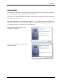
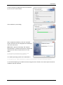
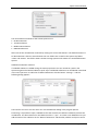
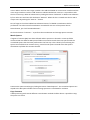
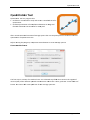
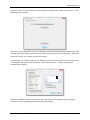
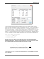
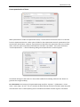
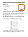
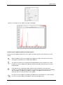
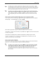
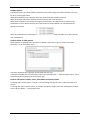
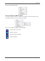
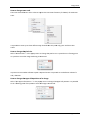
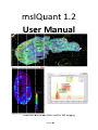
msIQu
m
uant 1.2 U er Maan
Use
nuaal CA1‐3 Cx TH
SN CP
Pu Evaaluation aand quanntitation tool for MS Imagging
Version A
AB Table of Contents Table of Contents Table of Contents .................................................................................................................................... 2 Legal and Regulatory Notices .................................................................................................................. 4 Protocol for Data Analysis ....................................................................................................................... 5 Conditions............................................................................................................................................ 5 Process flow......................................................................................................................................... 5 Spectra folder definition ..................................................................................................................... 6 Pixel definition ..................................................................................................................................... 6 Associated files .................................................................................................................................... 6 Installation ............................................................................................................................................... 7 Spectra Processing .................................................................................................................................. 9 Parameters ........................................................................................................................................ 10 Baseline correction with first quartile ........................................................................................... 10 Baseline subtraction and baseline denoising: Transform parameters .......................................... 10 Savitzky‐Golay filter for smoothing and differentiation ................................................................ 10 Noise calculation ........................................................................................................................... 10 Peak Picking ................................................................................................................................... 10 Recalibration ................................................................................................................................. 11 Processing .......................................................................................................................................... 12 Acquisition properties… ................................................................................................................ 12 Processing single fid file… .............................................................................................................. 12 Process spectra… ........................................................................................................................... 13 Spectra Normalization ........................................................................................................................... 14 Normalize Spectra ............................................................................................................................. 14 Match Spectra ................................................................................................................................... 16 Copy Structure ................................................................................................................................... 16 Create Structure ................................................................................................................................ 17 Quantitation Tool .................................................................................................................................. 18 Create standard curve ....................................................................................................................... 18 Create quantitation of tissue............................................................................................................. 22 XML Evaluation ...................................................................................................................................... 23 Perform xml evaluation ..................................................................................................................... 23 Pixel analysis ...................................................................................................................................... 24 msIQuant 1.2 User Manual Version AB Page 2 of 39 Table of Contents Spectra View .......................................................................................................................................... 25 How to open mass spectrum files ..................................................................................................... 25 How to zoom in and out and how to move spectra .......................................................................... 26 How to select a specific m/z and intensity range or set axis and spectra offset .............................. 27 How to measure m/z and intensity ................................................................................................... 27 Display options .................................................................................................................................. 28 How to delete or hide spectra ........................................................................................................... 28 How to edit spectra names, colors, line widths and spectra order .................................................. 28 How to edit the graph colors ............................................................................................................. 29 How to copy the image ..................................................................................................................... 30 How to copy the spectra within a specific m/z range ....................................................................... 30 How to select specific spectra peaks ................................................................................................. 30 How to set peak picking parameters ................................................................................................. 30 Image View ............................................................................................................................................ 31 How to open image xml files ............................................................................................................. 31 How to select different interpolation methods ................................................................................ 32 How to change color scale ................................................................................................................ 33 How to change the pixel size ............................................................................................................. 33 How to change the upper left position of an image ......................................................................... 33 How to change the parameters of the color scale, title and unit ..................................................... 34 How to save an image generated by Image View ............................................................................. 34 Examples of displaying a single or multiple m/z channels ................................................................ 35 Remove msIQuant Files ......................................................................................................................... 36 Remove Spectra Processing files ....................................................................................................... 36 Remove Bruker Files .......................................................................................................................... 36 Appendix – Abbreviations ..................................................................................................................... 37 Index ...................................................................................................................................................... 38 msIQuant 1.2 User Manual Version AB Page 3 of 39 Legal and Regulatory Notices Legal and Regulatory Notices Copyright © 2013 Biomolecular Imaging and Proteomics Group (BIP), Uppsala University. All rights reserved. All other trademarks are the sole property of their respective owners All Rights Reserved Reproduction, adaptation, or translation without prior written permission is prohibited, except as allowed under the copyright laws. Document History msIQuant 1.2 User Manual, version AB (November 2013) Warranty The information in this document is subject to change without notice. BIP is not liable for errors contained herein or for incidental or consequential damages in connection with the furnishing, performance or use of this material. Use of Trademarks The names of actual companies and products mentioned herein may be the trademarks of their respective owners. License for use and distribution msIQuant 1.2 is freeware software. msIQuant 1.2 can be used on any computer, including a computer in a commercial organization. msIQuant 1.2 is developed in C++ with Microsoft VS2010, MFC and .NET framework. At present time the source code is not open source. One doesn’t need to register or pay for msIQuant 1.2, but if the software is used for publication, please cite the following article: Källback P, Shariatgorji M, Nilsson A, Andrén PE. Novel mass spectrometry imaging software assisting labeled normalization and quantitation of drugs and neuropeptides directly in tissue sections. J Proteomics. 2012 Jul 27. [Epub ahead of print]. doi:10.1016/j.jprot.2012.07.034 msIQuant 1.2 User Manual Version AB Page 4 of 39 Protocol for Data Analysis Protocol for Data Analysis Conditions Version 1.2 of msIQuant is only working together with Bruker Daltonics flexImaging™ and the data format XMass. If the new Container data format is used it must first be converted with flex Data Converter. Further, only full MS in reflectron or linear mode can be analyzed. LIFT or FAST data can’t be analyzed in current version of msIQuant. Process flow The process flow below illustrates the overall protocol for the data analysis: Vendor of MALDI IMS software Spectra View Define ROIs of calibration spots and experimental tissue. Export the Display single spectra list from regions that contains information about the ROIs. spectrum or multiple spectra. Spectra Processing Perform spectra processing such as: baseline correction, denoising and subtraction, spectra smoothing and recalibration. Spectra Normalization Normalize spectra such as: non normalization, median‐, TIC‐, RMS‐ or labeled normalization. Create folder structures from the spectra list XML files and match normalized spectra with the structures. This process will create average spectra from each ROI defined by the spectra list. Quantitation Tool Select the ROI folder structure of the calibration spots. Extract peak information from peaks of interest. Create standard curve for quantitation. The standard curve is then implemented to the normalized spectra of the experimental tissue. An image xml file from the experimental tissue is created for further evaluation and display. XML Evaluation Image View Evaluate the image xml file. Following Display an image by the information from the image xml file. Information is generated: number of pixels; average quantified value; SD; RSD; min value; max value; pixel deviation analysis; pixel ratio calculation. msIQuant 1.2 User Manual Version AB Page 5 of 39 Protocol for Data Analysis Spectra folder definition To be able to use the programs in MALDI Tools the user has to understand the overall data structure. There are two different expressions that are used: spectra top folder and spectra folder. In the spectra folder are all the spectra for regions of interest (ROI) or spectra from different experiments. The spectra top folder though, contains one or several spectra folders. See the structure below. … DATA Spectra top folder Spectra folder 1 0_R00X006Y053 0_R00X006Y054 0_R00X006Y055 0_R00X006Y056 0_R00X006Y057 Spectra folder 2 0_R00X010Y077 0_R00X010Y078 0_R00X010Y079 0_R00X010Y080 0_R00X010Y081 Spectra folder 3 Spectra folder 4 The manual is also referring to spectrum folder. Spectrum folders are those that are contained in a spectra folder e.g. folder 0_R00X006Y053 is a spectrum folder. When the data analysis with the program suite in MALDI Tools has been performed there are three new folders in the spectra top folder: AVG, PeakList and StDev folders. … DATA Spectra top folder Spectra folder 1 Spectra folder 2 Spectra folder 3 Spectra folder 4 AVG PeakList StDev The AVG folder will contain the average spectra for each spectra folder. The StDev folder will contain the standard deviation spectra for each spectra folder and a noise calculation for each average spectra that includes local noise and average spectrum noise. The PeakList folder will contain the peak list for each average spectrum and extracted peak information file for a specific spectrum peak. Pixel definition The definition of a pixel in this user manual is the same as sampling position where a mass spectrum is acquired. Associated files List of file extensions and their associated programs:  *.cal – Mass spectrum recalibration file, associated with Spectra Processing  *.par – Labeled normalization parameter file, associated with Spectra Normalization  *.dat – Mass spectrum data file, associated with Spectra View msIQuant 1.2 User Manual Version AB Page 6 of 39 Installation Installation The installation of msIQuant is very simple and the whole package comes with a single self‐extracting file. The installation file can be downloaded at www.maldi.ms. The latest version of the installation is msIQuant 1.2.0.10 and the computer requirement is Windows operating system XP or higher. After downloading the file (current file name: msIQuant_1_2_0_10.exe) and store it on a place in the computer, double click on the file and it will self‐extract. A security warning dialog may appear since no valid digital signature is attached with the installation file. When the self‐extracting file starts the installation is prepared. A welcome screen appears. Click the “Next >” button to continue. msIQuant 1.2 User Manual Version AB Page 7 of 39 Installation Current settings are displayed. Start the installation by click on the “Install” button. The installation is proceeding. After completed installation, click the “Finished” button. Shortcut icons are displayed on the desktop and in the start menu. Note: When “Spectra Processing” and “Spectra Normalization” is used for the first time, look for the calibration list and/or the parameter list in the folder: <C:\Program Files\Biomolecular Imaging and
Proteomics Group\ProcessingParameters>
or in 64‐bit operating system such as Windows 7: <C:\Program Files (x86)\Biomolecular Imaging and Proteomics Group\ProcessingParameters> To uninstall msIQuant go into Add or Remove Programs that is found in the control panel. Search for msIQuant and then uninstall. msIQuant 1.2 User Manual Version AB Page 8 of 39 Spectra Prrocessing Specctra Pro
ocessin
ng Spectra Processing iss a program that perform
ms general sp
pectra ulting spectru
um is stored in each specctrum processing. The resu
with a name ccalled <xy.dat> and is loccated in the ssame folder folder w
hierarchy as the <fid
d> file. Below
w is an exampple of the hie
erarchy: 0_R00X0111U062 1 11Ref pdata acqu acqus fid SpectraProceessing.xml sptype xy.dat are: The specctrum processsing steps a
 Baselline correctio
on  Baselline subtracttion and denoising  Specttrum smooth
hing  Peak picking and Recalibration msIQuan
nt 1.2 User M
Manual Version A
AB
Pagge 9 of 39 Spectra Processing Parameters Baseline correction with first quartile The baseline correction is an algorithm that straightens out the baseline when the baseline of a spectrum is drifting. The method that is used to create a baseline is the simple moving first quartile (SMQ1). The only parameter to set in this function is the length of the moving frame. The value of this frame can be 0 – 20% of the total m/z channels and the default value is set to 10%. After creation of the baseline the baseline is subtracted with the spectrum. To avoid negative spectrum values the modulus of the largest negative value is added to all intensities for all m/z channels. Baseline subtraction and baseline denoising: Transform parameters The baseline subtraction and baseline denoising is performed with an algorithm called sorted mass spectrum transform (SMST). The noise part in the SMST transform is determined by three parameters, Cutoff, Cutoff intensity and Denoising level. If the intensity is higher than the Cutoff intensity at the Cutoff of the SMST transform, the transform is scaled down from 0 to the Cutoff to be equal as the set Cutoff intensity. The peak part of the SMST transform is subtracted by a value so the transform fits the Cutoff intensity. If the intensity is smaller at the Cutoff than the Cutoff intensity no processing is performed. If a more aggressive denoising shall be done the Denoising level is set higher than 1. The derivative at the Cutoff is calculated and is multiplied by the Denoising level. A new Cutoff is determined where this calculated derivative is located and the denoising is performed as described above. Savitzky‐Golay filter for smoothing and differentiation The spectrum smoothing is done with Savitzky‐Golay smoothing filter. The smoothing method can be with either average or 2nd degree polynomial. The frame of data points must also be defined and must consist of an odd number. The default value is set to smoothing of 2nd degree polynomial with a frame of 9 data points. Noise calculation The noise calculation is based on the SMST transform. In this part the SMST transformed is the m/z channels normalized from 0 to 1. The intensity is also normalized from 0 – 1. The transform is then derived. The parameter in the noise calculation, Noise cutoff, is the value of the derivative until the noise is considered to be localized. The default value of the derivative (Noise cutoff) is set to 0.05. All values after this cutoff is set to zero and the SMST is retransformed. The noise is then calculated as the root mean square (RMS) of all peaks in the noise. Peak Picking The peak picking algorithm is calculated as the signal to noise ratio (SNR) and the default value is set to 2. The reason to do the peak picking is to be able to do recalibration of the spectrum. The peak picking is done by deriving the spectrum. When the derivative is crossing the x‐axis from positive to negative value there might be a potential peak that is determined by the SNR. The peak itself is calculated by applying a 3d degree polynomial of the spectrum where the derivative is crossing the x‐
axis msIQuant 1.2 User Manual Version AB Page 10 of 39 Spectra Processing Recalibration When spectra are acquired during an MALDI imagine MS experiment they have to be recalibrated afterwards even if a calibration has been performed before an experiment. This is because of how some MALDI MS instrument is constructed. When a time of flight (TOF) MS is used the m/z will differ because of the difference in tissue and matrix thickness. The recalibration is performed against known peaks and the methods to this processing step are single calibrant recalibration, or multiple calibrant recalibrations with 1st or 2nd order. To do a 1st order recalibration at least two known peaks are required. For 2nd order recalibration at least three known peaks are required. For both 1st and 2nd order recalibration a calibration curve is generated with best fit against the calibrant. One point calibration can also be used if only one calibrant is in the list. The one point calibration will only shift the peaks. If a calibration before setting up an experiment has failed, it is possible to correct a spectrum if a mass shift has occurred with up to ±2 Da. This value is set in the main dialog, In the recalibration dialog it is possible to open a calibration file that contains the calibrant needed to perform the recalibration. The file extension for the calibration file is “*.cal”. To create a new calibrant list just add the name of the substance in the “Name of Substance” edit window, add the substance mass in Dalton and the tolerance in ppm. Push the “Add” button to add the calibrant in the list. It is possible to edit the list in two ways, delete all substances by clicking the button “Delete All” or delete one substance by first select one and then click the button “Remove”. When the list is created save the list with a unique name by pushing the “Save As…” button. Click the first or second order calibration and click the “OK” button. Depending on which spectra processing steps to be done one need to check the different steps to be done. The processing steps that can be selected are:  Baseline correction  Baseline subtraction/denoising  Smoothing  Peak picking  Recalibration msIQuant 1.2 User Manual Version AB Page 11 of 39 Spectra Processing Processing The different processing options are:  Acquisition properties  Processing single fid file  Process spectra Acquisition properties… To analyze the properties of a single pixel, click the button “Acquisition properties…” and select the fid file in the spectrum of interest. Below is an example of the information that is put together. Processing single fid file… To process a single spectrum, click the button “Process single fid file…” and select the fid file in the spectrum of interest. All processing steps are stored as CSV files and can be viewed by Spectra View. It is advisable to check the processed spectrum for some spots with Spectra View to confirm that the spectra processing is as expected. One can view the file SpectraProcessing.xml to check the numerical result from the different processing steps. The generated files are:  xy01_RawSpectrum.csv – Raw spectrum  xy02_Quartile1Spectrum.csv – Baseline of the raw spectrum  xy03_BaselineCorrSpectrum.csv – Corrected raw spectrum  xy04_TransformSpectrumNormMZ.csv – SMST of the corrected raw spectrum  xy05_TransformSpectrumNormMZBaselineProc.csv – SMST with cutoff  xy06_TransformNormMZNormInt.csv – SMST with cutoff and normalized intensity from 0 – 1  xy07_TransformSpectrum.csv – SMST with cutoff and the intensities corresponding masses  xy08_InvertedTransformSpectrum.csv – Retransformed SMST spectrum  xy09_GentleSmoothingSpectrum.csv – Spectrum smoothed with Savitzky‐Golay smoothing filter  xy10_DerivativeSpectrum.csv – Derivative of smoothed spectrum  xy11_SpectrumNoise.csv – Spectrum noise with removed peaks  xy12_DerivativeNoise.csv – Derivative of noise spectrum msIQuant 1.2 User Manual Version AB Page 12 of 39 






Spectra Processing xy13_PeakNoise.csv – Peak noise indication spectrum xy14_ValleyIndication.csv – Valley indication of smoothed spectrum xy15_BaselineSmooth.csv – Baseline of smoothed spectrum xy16_RecalibratedSpectrum.csv – Recalibrated spectrum PeakList.csv – Peak list before recalibration PeakListPost.csv – Peak list after recalibration SpectraProcessing.xml – The result of the spectra processing Process spectra… To process spectra in a top folder, click the button “Process spectra…” and select the top folder. During this process a xy.dat file and a SpectraProcessing.xml file are created in each spectrum folder. The progress bar will indicate how much of the spectra that have been processed. msIQuant 1.2 User Manual Version AB Page 13 of 39 S pectra Norm
malization Specctra Normaliza
ation Spectra Normalizatio
on is a progra
am that:  Norm
malize spectra with different methodss.  Makees average sp
pectra from ROI and/or ttissue experiments.  Matcches normalizzed spectra tto later definned ROI.  Copiees spectra structures whe
en different normalizatio
on method is perrformed on ssame experim
ment.  Creattes spectra structures fro
om spectra liist from regio
ons. unning this p
program, run
n Spectra Proocessing to create <xy.da
at>. Before ru
Normallize Spectraa After thee spectra pro
ocessing with
h Spectra Proocessing are performed, normalizatioon and creattion of average spectra is do
one with Spe
ectra Norma lization – No
ormalize Specctra. When tthe normalization is nsities are resstored in resspect to the n
normalizatio
on method foor each specttrum. performed the inten
Thereforre must the eexperimentss from the coontrol tissue and the experiment tissuue be norma
alized at the samee time. The sspectra top ffolder must ccontain specctra folders fo
or control tisssue and experimental tissue. When the b
button “Norm
malize Spectrra…” is presssed the follow
wing window
w appears: msIQuan
nt 1.2 User M
Manual Version A
AB
Page
e 14 of 39 Spectra Normalization The normalization methods for the overall spectrum are:  No Normalization  TIC Normalization  Median Normalization  RMS Normalization Select one of the normalization methods by clicking one of the radio buttons. The default selection is TIC Normalization. After the normalization two new folders are created in the spectra top folder: <AVG> and <StDev>. The folder <AVG> contains average spectra and <StDev> the standard deviation spectra. Labeled normalization method: If a labeled substance is added during the tissue preparation one can normalize a peak in the spectrum against this labeled substance peak. Up to 10 labeled substances can be labeled normalized in the same spectrum. To add a list of labeled substances click the button “settings…” and the following dialog appears: The interface is more or less the same as in the Recalibration dialog in the program Spectra Processing. It is possible to open a labeled ion file that contains the calibrant needed to perform the recalibration. The file extension for the labeled ion file is “*.par”. To create a new labeled ion list just add the name of the substance in the “Name of Substance” edit window, add the analyte ion center msIQuant 1.2 User Manual Version AB Page 15 of 39 Spectra Normalization mass in Dalton and the mass range in Dalton. Also add the labeled ion center mass in Dalton and the mass range in Dalton. Push the “Add” button to add the labeled ion in the list. It is possible to edit the list in two ways, delete all substances by clicking the button “Delete All” or delete one substance by first select one and then click the button “Remove”. When the list is created save the list with a unique name by pushing the “Save As…” button. Do not forget to check the labeled normalization button if a labeled normalization shall be performed. If no other overall normalization is needed for the rest of the spectra like TIC Normalization, just click “No Normalization”. Click on the button “Continue…” to perform the normalization and average spectra creation. Match Spectra If regions of interest (ROI) have been defined and the spectra are located in a new top folder contained with the different ROI spectra folders one need to match these new spectra with the normalized spectra that has been performed in the first step. This is done by first selecting the spectra source folder that contains the e.g. control tissue spectra. Second select the spectra destination top folder that contains the ROI. Continue the spectra matching by clicking the button “Match Spectra”. The normalized spectra are copied to the ROI spectra folders and an average spectrum is calculated for each ROI. Copy Structure If data processing with several different normalization methods shall be done it is possible to copy the spectra structure. msIQuant 1.2 User Manual Version AB Page 16 of 39 Spectra Normalization It is possible to copy a whole top structure or just a plain structure as a single spectrum folder. The information that is copied is just folder structure, not the underlying data. Create Structure To create folder structures containing ROI and their spectra, select first the spectra list from regions xml file (created by Bruker Daltonics flexImaging™). Select also the destination top folder where the ROI folders will be created. Click on the button Create Structure to continue. To fill the created folder structures with normalized spectra, go back to the tab Match Spectra and continue. msIQuant 1.2 User Manual Version AB Page 17 of 39 Quantita
ation Tool Quan
ntitatio
on Tool Quantitaation Tool is a program that:  Perfo
orms a conceentration study and creattes a standarrd curve for quantitation.  Perfo
orms quantitation of tissu
ue/ROI and ccreates an im
mage xml file w
with substancce concentra
ation for eachh pixel. n of average spectra the next step is tto perform sstandard curvve and After normalization aand creation
quantitaation of expeeriment tissue. unning this p
program, run
n Spectra No rmalization to create ave
erage spectrra. Before ru
Create sstandard cu
urve er that contaains the regio
ons of The first step in creation of a standard curve is to select tthe top folde
otted concenntrations. W
When this is done, push thhe “Create Pe
eak List” interest (ROI) of the different spo
will create pe
eak lists of eaach average spectrum. button. TThis action w
msIQuan
nt 1.2 User M
Manual Version A
AB
Page
e 18 of 39 Quantitation Tool The second step is to select the peak of interest by pushing the button “Select m/z of a Peak…”. The following window appears: Click on the combo box button and a list of all peaks and their centroid mass and average peak height will appear. Select the peak mass of interest and click on the button “Extract Single Mass”. After peak extraction click the “Exit” button to close the window. The third step is to create a standard curve based on the mono isotopic peak from the substance that is investigated. Continue to click the button “Create Standard Curve…” and the dialog Create Standard Curve appears: Enable the checkbox “Export Concentration Data” and then click on the big button with a graph bitmap on and the next dialog Concentration Study will appear. msIQuant 1.2 User Manual Version AB Page 19 of 39 Quantitation Tool To find the extracted peak from the second step go to the top folder and the into the <PeakList> folder, there is the extracted peak file (e.g. the file <Peak_281.2034.csv>). To make it easy to find the file the mass of the centroid peak is attached to the file name. In the list box the regions from the concentration spots appear. To edit the amount of added substance double click on the region name and edit the correct amount in the edit window that appears and enter the return key. If one spots should be an outlier single click on the region and click on the button “Remove”. The slope, intercept and R2 for the standard curve are updated simultaneously. There are three different selections that can be made to calculate the concentrations:  The amount of substance alone  The amount per mm3 tissue  The amount per mg tissue Select the concentration option in the group box “Select Type for Slope/Intercept Calculation”. Depending on the selection, measure the average spot diameter, tissue thickness and tissue density. For convenience the selected tissue volume and tissue mass will be calculated. Tip! If the whole spot is selected and the pixels in the spot are extracted, count the pixels and multiply them with the x and y resolution to calculate the area. The diameter from the average area of the spots can be calculated by the formula and is easier then predict the diameter by measuring the picture. To view the standard curve, click on the button with bitmap picture of a graph. Below is an example of how it looks like. msIQuant 1.2 User Manual Version AB Page 20 of 39 Quantitation Tool To force the standard curve to go through origin, enable the check box “Zero Intercept”. There is also another option to form a 2nd order polynomial by enable the check box “Polynomial Regression”. This might be handy if low amounts of the substance are spotted and ion suppression is present. If this option is selected the “Zero Intercept” cannot be selected in this version of the program. When all settings are done click on the “OK” button and the settings will be transferred to the previous dialog “Export Concentration Data”. It is now possible to generate an image xml file for the concentration spots. A selection that influences the image xml file is the “Region Parameters”. If a uniform concentration is required per spot, select “Average Data per Region”. Otherwise leave as is. Click the “OK” button to generate the image xml file. msIQuant 1.2 User Manual Version AB Page 21 of 39 Quantitation Tool Create quantitation of tissue When quantitation is made on experimental tissue, it can be done to the entire tissue or on the ROI from the experimental tissue. Select spectra folder for the experimental tissue if quantitation of the whole tissue shall be done. However, if quantitation of the ROI of the experiment the tissue shall be done, select the spectra top folder and enable the checkbox “Top Folder”. Then press the button “Create Quantitation ...” and the following dialog Create Quantitation of Tissue appears: The default settings are the same as in the Create standard Curve dialog. Click the “OK” button to generate the image xml file(s). For information! The naming of the generated image xml file is “ExpConc” + foldername + center mass + mass range + H or A + P or R. H is when the peak intensity has been used and A when the peak area has been used. P is when pixel by pixel is calculated and R when a whole region is calculated. msIQuant 1.2 User Manual Version AB Page 22 of 39 XML Evvaluation XMLL Evaluaation XML Evaaluation is a p
program that performs ccalculation off the generateed xml file frrom the proggram Quantittation Tool. TThe informattion and calcculation of an
n xml file aree:  Numb
ber of pixels  Averaage quantifieed value  Stand
dard deviatio
on (STD) of th
he quantifiedd value  Relattive standard
d deviation (R
RSD) of the qquantified vaalue  Min vvalue of the quantified va
alue  Max vvalue of the quantified vvalue  Pixel deviation an
nalysis (PDA)  Pixel ratio calculaation (PRC) unning this p
program, run
n Quantitatioon Tool to creeate image xxml file(s). Before ru
Perform
m xml evalu
uation Select an
n image xml file and clickk on the buttton “Evaluate
e…” to evalu
uate the file. The next dia
alog box will appeear: msIQuan
nt 1.2 User M
Manual Version A
AB
Page
e 23 of 39 XML Evaluation The information in the dialog is automatically copied to the clipboard to easily past into e.g. Microsoft Excel. Below is an example from Excel when the evaluation is pasted: Pixel analysis The program makes analysis of neighbor pixels how much they differ from each other with by Pixel Deviation Analysis and Pixel Ratio Calculation. Below is a description of the algorithms: Pixel Deviation Analysis p-2,-2
p-1,-2
p0,-2
p1,-2
p2,-2
The resolution does not matter when performing a pixel deviation analysis with quadratic pattern since the relative p-2,-1
p-1,-1
p0,-1
p1,-1
p2,-1
distance is always the same. p
p
p
p
p
-2,0
-1,0
0,0
1,0
2,0
The algorithm works in the way that the distance to all eight neighbors is the same and is represented by the dotted circle p
p
p
p
p
-2,1
-1,1
0,1
1,1
2,1
around the central pixel. p-2,2
p-1,2
p0,2
p1,2
p2,2
Each pixel is named with x and y index px,y . For each pixel there is an intensity also named with x and y index Ix,y . The abbreviation of Pixel Deviation Analysis is for short PDA. Differences for each neighbor pixel are calculated: D1,0 = I1,0 ‐ I0,0; D0,1 = I0,1 ‐ I0,0; D‐1,0 = I‐1,0 ‐ I0,0; D0,‐1 = I0,‐1 ‐ I0,0 …except for the corner pixels where the differences are divided by the square root of 2. D1,1=(I1,1 ‐ I0,0) /√2 ; D‐1,1=(I‐1,1‐ I0,0) /√2 ; D‐1,‐1=(I‐1,‐1 ‐ I0,0) /√2 ; D1,‐1=(I1,‐1 ‐ I0,0) /√2 ; The root mean square (RMS) is then calculated of the eight differences (the PDA is equal to the RMS). PDA  RMS 


1 2
D1, 0  D02,1  D21, 0  D02, 1  D12,1  D21,1  D21, 1  D12, 1 8
Pixel Ratio Calculation The Pixel Ratio of a region of interest (ROI) is the average Intensity from the pixels divided by the average PDA of the pixels. msIQuant 1.2 User Manual Version AB Page 24 of 39 Specctra View Specctra Vie
ew Spectra V
View is a pro
ogram that d
displays masss spectra file
es. It is capable to display fo
ollowing filess: dat mass speectra files.  star.d
 star.ccsv mass speectra files.  fid raaw mass specctrum files th
hat is createdd by Bruker Daltonics flexControl™. mat of the daat and csv file
es are text fi les were the
e first line can
n be a headeer that conta
ains The form
informattion like “m//z” and “Intensity”. The ffile must contain only two columns w
where the firsst column iis the mass aand the second column iss the intensity. The decim
mal separatioon must be a
a dot ‘.’ (character value 0x2e) and the co
olumn separration characcter can be a
a tab (charact
cter value 0x0
09), space ‘ ‘ (character vvalue 0x20) o
or a comma ‘‘,’ (characterr value 0x2c). The line muust end with carriage return (ccharacter vallue 0x0d) and line feed (ccharacter value 0x0a). How to open masss spectrum files Since *.d
dat files are aassociated w
with Spectra V
View it will sstart Spectra View and oppen the file d
directly when do
ouble clickingg on it in exp
plorer. Norm ally *.csv file
es are associated with W
Windows Exce
el but to open it ffrom exploreer, right click on the *.csvv mass spectrum file and click on “Se nd To” and sselect “Spectraa View” that is in the men
nu. To open a fid mass sp
pectrum raw
w file in exploorer, right click on the fid fiile and selectt “Open” in tthe menu annd select Spe
ectra View in the Program
ms list. It is also possible to sstart Spectra
a View and riight click on the window and the folloowing popup
p menu appears: Open Spectru
um…” in the popup men u or just pre
ess <Ctrl+O> to open a m ass spectrum
m. It is Select “O
also possible to open
n several spe
ectra with m ultiple selecttions. Once a
a spectrum iss opened it is possible to open onee or several m
more spectraa. If spectra have been edited it is poossible to reo
open menu. them again by selectting “Recent Spectra” in tthe system m
msIQuan
nt 1.2 User M
Manual Version A
AB
Page
e 25 of 39 Specctra View mass spectruum is displayyed: Below is an example of how a m
How to zoom in an
nd out and how to mo
ove spectra
During the zoom opeeration different cursors appear and their specific zoom operration can ta
ake action: When the ZZoom in m/z cursor appeears it is posssible to zoom
m in and out tthe m/z axis by d forth. moving thee scroll wheel on the mouuse back and
The Zoom in intensity cursor appearrs by pressin
ng <Ctrl> key on the keybboard. It is th
hen d out the inteensity axis byy moving the
e scroll wheeel on the mouse possible to zoom in and
back and fo
orth. If the Zoom
m in m/z or in
ntensity cursoors appears and the specctrum mass sspectrum is o move the sspectrum in both m/z and intensity ddirection by h
holding zoomed, it is possible to
down the leeft mouse bu
utton and moove the mou
use on the sp
pectrum areaa. Once the spectrum sttarts to movve, the Hand cursor appe
ears. The Zoom in cursor app
pears by presssing the <Alt> key on the keyboard. It is then po
ossible m by selectinng the zoom area with th
he mouse. to zoom in the spectrum
msIQuan
nt 1.2 User M
Manual Version A
AB
Page
e 26 of 39 Specctra View axis arrow cu
ursor appearss when holding the curso
or over the m
m/z axis. Dou
uble The Mass a
click with th
he left mouse button on the m/z axiss to rescale to the full m//z range. If th
he mass spectrum iss zoomed it is possible too move the spectrum in m
m/z directionn by holding down the left mouse button a
and move th e mouse on the m/z axiss. The Intensity axis arrow
w cursor appeears when holding the cu
ursor over thhe intensity a
axis. Double click with the le
eft mouse buutton on the intensity axis to rescale tto the full intensity range. If thee mass specttrum is zoom
med it is posssible to move
e the spectruum in intensity direction byy holding down the left m
mouse butto
on and move the mouse oon the intensity axis. How to select a specific m/z a
and intensitty range or set axis and spectra ooffset To set a specific m/z and intensitty range, righht click the right mouse b
button and cclick “Set m/zz and menu or just press <Ctrl+
+R>. intensityy range…” in the popup m
Set the vvalues to gett specific range of m/z annd intensity aand click the “OK” buttonn. If the speectrum is clo
ose to the zero intensity it is possible
e to set a neg
gative axis offfset value to
o be able to “lift up” the specttrum. If severaal spectra aree displayed itt is possible tto separate tthem by settting the specctra offset. If a peakk is investigatted and it is the highest iin the whole
e spectrum, itt is possible to set a new
w maximum intensity tto zoom out the spectrum
m. How to measure m
m/z and inte
ensity The information abo
out m/z and iintensity is s hown all the
e time when the mouse iss moved ove
er the measure thee m/z and inttensity differrence: graph arrea. It is also possible to m
The Measure cursor appears when pressing <Sh
hift> key on tthe keyboardd and is used
d for or to a speciffic peak, pre ss down the left measuring Δm/z and Δintensity. Moove the curso
mouse buttton and movve the cursorr to a new pe
eak and relea
ase the mousse button. A message bo
ox appears w
with the inforrmation about the Δm/z and Δintenssity. The information
n is automatically copiedd to the clipb
board to be able to paste it directly to
o e.g. Microsoft EExcel. msIQuan
nt 1.2 User M
Manual Version A
AB
Page
e 27 of 39 Spectra View Display options The display options are; Show Gridline, Show Zero Axis, Show Legend, and Show baseline. They can be all set in the popup menu. When Show Gridline is set it displays the major gridline for both intensity and m/z. When Show Zero Axis is set it displays the zero intensity axis in the spectrum. When Show Legend is set it displays the legend of the spectra. The legend can be moved in the window but is set in default position when the window is resized. Below is an example how the legend can look like. When Show baseline is set the baseline is displayed in the same color and width as its spectrum but with a dashed line. How to delete or hide spectra When spectra are opened and if one wants to delete a spectrum or spectra; select the “Delete Spectrum…” from the popup menu. Check the spectrum that is going to be removed and click “OK”. If one wants to hide one or more spectra; select the “Hide Spectrum…” from the popup menu. Check the spectrum that is going to be hid and click “OK”. How to edit spectra names, colors, line widths and spectra order To change order of the spectra, click on an item and drag and drop the item to the new position in the list. To change the spectra names, colors, line widths and spectra order; select the “Edit Spectrum Name, Color and Line Width…” in the popup menu. msIQuant 1.2 User Manual Version AB Page 28 of 39 Spectra View To change the name, color and line width of a spectrum, double click on the item and the following dialog window is shown: Edit the spectrum and click “OK”. How to edit the graph colors To customize the graph colors, select the “Edit Graph Color…” in the popup menu. To change a color, double click on the item and select a new color: msIQuant 1.2 User Manual Version AB Page 29 of 39 Spectra View How to copy the image To copy the graph image to the clipboard, select “Copy Image” in the popup menu and paste it directly to e.g. Microsoft PowerPoint. How to copy the spectra within a specific m/z range To copy the spectra in the window to the clipboard, select “Copy Spectra” in the popup menu and paste it directly to e.g. Microsoft Excel. How to select specific spectra peaks Zoom in and display the peaks of interest. To select the Peak cursor, click once on the <Tab> key. Then click on the left side of the peak and the graph will display information of the centroid m/z, centroid intensity, the peak area and the signal to noise ratio. The information about the selected peaks is automatically copied to the clipboard to be pasted to e.g. Microsoft Excel. How to set peak picking parameters To change parameters for peak picking, select the “Peak Option…” in the popup menu. Edit the signal to noise ratio for peak selection. Edit the mass frame to be able to select a group of peaks. msIQuant 1.2 User Manual Version AB Page 30 of 39 Image View Imagge View
w Image View is a proggram to displlay an imagee xml file gen
nerated on Tool. from thee Quantitatio
The Imagge View is in
n its present sstate more oor less a prottotype of displayin
ng images. Th
he goals with
h this softwaare were to investigate renderin
ng principle, interpolation
n methods, ccolor scale implemeentation and
d overlay of u
up to three ddifferent images. The image xm
ml file is com
mpatible with
h Bruker Dalttonics flexIm
maging™ and can imported ass well. The rend
dering technology is calle
ed Silk‐Screeen rendering.. The bitmap
p image that is displayed is transferrred from thee original ima
age that is veectorized. How to open imagge xml files When th
he Image Vieew has starte
ed a small im
mage with 4x4
4 pixels is vie
ewed. The im
mage comes from the article: B
Bicubic interp
polation from
m Wikipedia (http://en.w
wikipedia.org
g/wiki/Bicub ic_interpolation). It is posssible to open
n an image xm
ml file in sevveral differen
nt ways. If the program iss already ope
en one can dragg and drop an
n image xml file or open the image xml file from a popup me nu by right cclick the window.. If the imagee xml file is liisted in the eexplorer one
e can open th
he file by righht clicking on
n the file and further click on ““Send To”. msIQuan
nt 1.2 User M
Manual Version A
AB
Page
e 31 of 39 Image View Below is the popup m
menu displayyed: How to select diffe
erent interp
polation meethods The defaault interpolaation method of an imagge is nearest‐‐neighbor. To
o change thee method, click on the Interrpolation and
d select one of four interrpolation me
ethods. Below is the four diffferent interp
polation metthods displayyed: Nearesst‐neighbor interpolatioon Bilineaar interpolattion Bilineaar Color Blend interpolatiion on Bicubicc interpolatio
msIQuan
nt 1.2 User M
Manual Version A
AB
Page
e 32 of 39 Image View How to change collor scale There arre eleven diffferent color scales to exppress the intensities for o
one m/z channnel, all with
h linear scale. but only with
h red, green and blue color It is posssible to view up to three different m//z channels b
scales. How to change the
e pixel size Select “SSet Pixel Sizee…” in the po
opup menu t o change the
e pixel size. It is possible set a floating point as a pixeel size since tthe image rendering is veectorized. In present version off the softwarre a pixel is ssquared so itt is not possible to set diffferent value
es of x and y dirrection. How to change the
e upper leftt position o
of an image
Select “SSet Upper Leeft Position…” in the popuup menu to change the u
upper left poosition. It is p
possible to set a ffloating poin
nt of the posiition since thhe image is vvectorized. msIQuan
nt 1.2 User M
Manual Version A
AB
Page
e 33 of 39 Image View How to change the parameters of the color scale, title and unit To change the value of the min and max intensity, select the “Set Min & Max Intensity” in the popup menu. To return to the default intensities, check the “Set Default Intensities” and click on OK button. It is also possible to change the title and the unit of the color scale. How to save an image generated by Image View The present version of msIQuant has no export possibility of Image View. The best way to save an image is to have the focus on Image View and to press <Alt> + <PrtScn> to copy the image to the clipboard. Then paste the image to the software where you want to show the image. msIQuant 1.2 User Manual Version AB Page 34 of 39 Image View Examples of displaying a single or multiple m/z channels Below are two examples of images. The first image displays a single m/z channel. The second image displays two different m/z channels and how they are distributed in the tissue. msIQuant 1.2 User Manual Version AB Page 35 of 39 Reemove msIQu
uant Files Remove mssIQuan
nt Files
Remove msIQuant Files is a proggram that rem
moves msIQuant n they are no
ot needed anny longer. It is also generateed files when
possible to remove rredundant da
ata when it iis not needed any o save disk space. longer to
Removee Spectra Processing fiiles Spectra Processing ggenerates xy..dat files in eevery spectru
um folder. To
o remove theese files whe
en they needed any longer, selecct the spectraa top folder where they are containeed, check “Re
emove are not n
xy.dat Fiiles” and click on the “Re
emove” buttoon. The proggress bar tells when the eerase operattion is complete. on generatess normalizedd CSV files. To
o remove the
ese files wheen they are n
not Spectra Normalizatio
needed any longer, sselect the spectra top follder where they are conttained, checkk “Remove on the “Rem ove” button. The progress bar tells w
when the era
ase Normalizzed CSV Filess” and click o
operatio
on is complette. Spectra Normalizatio
on also generates the fol ders; “AVG”, “StDev” and “PeakList””. To remove these folders w
with their content, selectt the spectraa top folder w
where they a
are containedd, check “Remove Folders C
Containing A
Average Filess etc.” and cl ick on the “R
Remove” buttton. The proogress bar te
ells when the erase operation is complete. Removee Bruker Filles When RO
OI spectra arre copied all informationn including raaw files etc are copied ass well. This informattion is not neeeded when running msIIQuant, only the empty sspectrum fol ders. To reduce the disk spacce it is possib
ble to removve this underrstructure. To
o do this, select the specctra top folde
er where they are contained, ccheck “Remo
ove Understrructures” an
nd click on the “Remove”” button. The
e hen the erase
e operation is complete. progresss bar tells wh
hole experim
ment shall bee erased it is possible to d
do this by, seelecting the sspectra When a copy of a wh
emove Comp
plete” and cliick on the “R
Remove” top foldeer where thee experimentt is containe d, check “Re
button. TThe progresss bar tells wh
hen the eras e operation is complete. msIQuan
nt 1.2 User M
Manual Version A
AB
Page
e 36 of 39 Appendix – Abbreviations Appendix – Abbreviations Abbreviation Explanation CSV IMS m/z MALDI MS R2 PDA PRC RMS ROI RSD SD SMST SMQ1 SNR TIC TOF xml Comma‐Separated Values Imaging Mass Spectrometry Mass to charge ratio Matrix‐Assisted Laser Desorption/Ionization Mass Spectrometry Coefficient of determination Pixel Deviation analysis Pixel Ratio Calculation Root Mean Square Region of Interest Relative Standard Deviation Standard Deviation Sorted Mass Spectrum Transform Simple Moving First Quartile Signal to Noise Ratio Total Ion Current Time of Flight eXtensible Markup Language msIQuant 1.2 User Manual Version AB Page 37 of 39 Index L Index Labeled Normalization A M Acquisition properties Average spectra Average quantified value 12 15 23 10 10 10 32 32 32 C Centroid mass Color scale Copy structure Create structure Cutoff Cutoff intensity 19, 20, 30 32 16 17 10 10 D Denoising level Display mass spectra 10 25 19 F File extensions 6 G Gridline 28 I Image xml file Installation of msIQuant Interpolation methods msIQuant 1.2 User Manual 16 15 27 Nearest‐neighbor interpolation No Normalization Noise calculation 32 15 10 P Peak height Peak mass Peak picking Pixel Pixel Deviation Analysis Pixel Ratio Calculation Pixel Size Process flow Process spectra Processing single fid file 19 19 10 6 24 24 33 5 13 12 Q Quantitation 18, 22 R E Extracted peak Match spectra Median Normalization Measure m/z and intensity N B Baseline denoising Baseline correction Baseline subtraction Bicubic interpolation Bilinear interpolation Bilinear Color Blend interpolation 15 18, 23, 31 7 32 R2 Recalibration Region name Remove complete Remove normalized CSV files Remove understructures Remove xy.dat files RMS Normalization 20 11 18 36 36 36 36 15 S Savitzky‐Golay smoothing filter Simple moving first quartile Sorted mass spectrum transform Spectrum smoothing Version AB 10 10 10 10 Page 38 of 39 Spectrum folder Spectra folder Spectra top folder Standard curve Index 6 6 6 17, 19 T TIC Normalization 15 Z Zoom in intensity Zoom in mass 25 25 msIQuant 1.2 User Manual Version AB Page 39 of 39