1
The MetabolomeExpress User's Guide (v 1.0)
By Dr Adam J. Carroll
QUICK START Load a dataset by left-clicking or right-clicking (or control-clicking if you are using a
single-button mouse on an Apple computer) on the experiment folder and left-clicking
'Load Folder Contents'
Table of Contents 1 MetabolomeExpress: Getting started .....................................................................4 1.1 Structural overview ...........................................................................................4 1.2 Public vs. private data access ..........................................................................5 1.3 Obtaining your own MetabolomeExpress data repository: Registration ...........5 1.4 Uploading and managing your datasets via FTP..............................................6 1.4.1 Logging in ..................................................................................................6 Step 1 - Create a data folder for the experiment ....................................................6 Step 2 - Upload raw GC/MS files ...........................................................................6 Step 3 - Perform Data Import and Peak Detection .................................................7 Step 4 - Upload sample information table: .............................................................7 Step 5 - Upload a retention index calibration file .................................................. 10 1.4.2 Choosing a research area and importing sample information.................. 11 1.5 Building and using custom Mass Spectral and Retention Index (MSRI)
libraries ....................................................................................................................13 1.5.1 An overview of the MetabolomeExpress MSRI library format .................. 13 1.5.2 Creating MSRI libraries from AMDIS .MSL files ...................................... 15 1.5.3 Adding metadata to MSRI libraries .......................................................... 18 1.5.4 Displaying and Validating MSRI Libraries with MSRI Library Manager ... 20 1.5.5 Using Analyte Annotations Tables to customise data filtering ................. 20 1.6 Supported Data Formats (including example files)......................................... 22 1.6.1 The main MetabolomeExpress metadata exchange format
(*_METADATA.TXT) ............................................................................................ 22 1.6.2 Raw GC/MS data: NetCDF and the MetabolomeExpress eXtracted Ion
Chromatogram (.XIC) format ................................................................................ 27 2 1.6.3 Peak list tables (.PEAKLIST) ................................................................... 27 1.6.4 MSRI library matching report tables (.MATCHREPORT)......................... 28 1.6.5 Data matrices (.mzrtMATRIX) .................................................................. 29 Re-analysis of publicly disseminated data using Database Explorer ................... 31 2.1 Getting an overview of the database with the Database Statistics panel ....... 31 2.2 Finding experiments of interest using ResponseFinder ................................. 32 2.3 Comparing metabolite response patterns across multiple publications using
MetaAnalyser ........................................................................................................... 33 2.4 Identifying phenocopies using PhenoMeter (in development) ........................ 36 3 Processing and analysis of experimental GC/MS datasets with Experiment
Explorer ....................................................................................................................... 38 3.1 Example dataset: Timecourse metabolomic analysis of plant cells treated with
Antimycin A .............................................................................................................. 38 3.2 Loading a dataset........................................................................................... 38 3.2.1 4 5 Loading a dataset from the Navigation panel .......................................... 38 3.3 Using the Raw Data Viewer ........................................................................... 39 3.4 The raw data viewer control panel ................................................................. 40 3.5 Zooming in and out ........................................................................................ 41 3.6 Viewing mass spectral scans ......................................................................... 42 3.7 tool
Finding differentially expressed peaks using the chromatographic statistical
42 Data import and peak detection (registered users only) ....................................... 43 4.1 A Guide to the MetabolomeExpress PeakFinder Algorithm ........................... 44 4.2 The Peak Detection Control Panel ................................................................. 45 MSRI library matching .......................................................................................... 46 5.1 How to conduct an MSRI library matching process ........................................ 46 Mass-Spectral Tag (MST) reconstruction and the MSRI library matching process ..47 5.2 6 Interacting with MSRI library matching results ............................................... 47 Statistics and data exploration ............................................................................. 49 6.1 Construction of data matrices from MSRI library-matching reports ................ 50 6.1.1 Some notes on normalisation and quality control .................................... 50 6.1.2 Raw data-assisted missing value replacement ........................................ 51 6.1.3 How to build a data matrix using the Match Report to Data Matrix tool ... 51 6.2 Matrix renormalisation .................................................................................... 54 6.3 Using the interactive matrix explorer .............................................................. 55 6.4 Comparative statistics .................................................................................... 56 6.5 Principal Components Analysis (PCA) ........................................................... 58 6.6 Hierarchical Cluster Analysis (HCA) ............................................................... 60 6.7 Correlation network construction .................................................................... 63 6.8 Submitting a dataset to the main database of metabolite response statistics 65 7 APPENDIX A – Interpretation of MetabolomeExpress Metadata Validation
Templates ................................................................................................................... 67 7.1 Background .................................................................................................... 67 7.2 Interpretation of MetabolomeExpress Metadata Template Files .................... 67 7.3 Validation Codes ............................................................................................ 69 7.4 Data types and associated configuration parameters .................................... 69 1 MetabolomeExpress: Getting started 1.1 Structural overview MetabolomeExpress is comprised of three interacting layers:
1. An FTP repository where registered users may upload and manage
their own GC/MS datasets
2. A MySQL database that stores general metabolite information and
metabolite response statistics from datasets present in the qualitycontrolled MetabolomeExpress database of metabolite response
statistics.
3. A web interface to interact with data present in the FTP repository and
MySQL database
Figure 1. Structural overview of MetabolomeExpress
1.2 Public vs. private data access MetabolomeExpress houses both public and private data (including GC/MS libraries).
Public data is accessible to anonymous users (ie. users automatically logged in as
'guest') via the web interface. Private data may only be accessed by registered users
who are logged in and have permission to access the private data (see Section 1.3
below for details).
1.3 Obtaining your own MetabolomeExpress data repository: Registration In order to analyse and share your own GC/MS datasets with MetabolomeExpress,
you must first register to obtain a username and password.
Registration is FREE.
Once your application to register has been received, you will be contacted by email to
determine whether you wish to create a new repository (and if so, what you want to
call the repository) or simply to join an existing repository. If you wish to join an
existing repository, we will require authorisation (via email) from the original creator of
that repository. It IS possible for you to have your own repository and also have
access to another repository via the web-interface - we just need to receive an email
request to give you repository access permissions from the owner of the other
repository. NOTE: Each registered username will obtain FTP access to only one
repository. If you wish to upload data to another repository, you must obtain the
username and password from an FTP user of that repository or register for another
username and password for use with that FTP repository.
1.4 Uploading and managing your datasets via FTP 1.4.1 Logging in To upload and manage your datasets via FTP, you will need an FTP client program.
We use the free FTP client, FileZilla, but most FTP clients should work fine. To
connect to your FTP repository, enter the following into your FTP client program:
Hostname: www.metabolome-express.org
username: your username
password: your password
and connect.
Once connected, you should see your repository.
This screenshot below shows an example of the result of logging in as AdamC using
FileZilla:
Once connected, there are a few simple steps to create a new experiment:
Step 1 ‐ Create a data folder for the experiment: Open either your public or internal
data folder and create a new subfolder with the name of the folder being the name of
the experiment (eg. 'Nutrient supplementation timecourse 1').
Step 2 ‐ Upload raw GC/MS files: Copy all the raw NetCDF/ANDI MS/AIA GC/MS files
(.CDF) for that experiment into the folder you just created. If you don't have your files
in NetCDF format, you should be able to export them from your instrument
manufacturer's data processing software.
HINT: It will make things easier for everyone if you name your files descriptively rather
than with meaningless numbers or letters. Name your files something like
'20091015_Nutritional Regime A_Day 1_Replicate 1.CDF', '20091015_Nutritional
Regime A_Day 1_Replicate 2.CDF' etc. (where the first 8 numbers represent the date
on which the batch sequence of GC/MS runs began, in YYYYMMDD format) rather
than something like '1.CDF', '2.CDF' etc.
Step 3 ‐ Perform Data Import and Peak Detection: Now, log in to
MetabolomeExpress and you should be able to find your new experiment folder
containing your data files in the 'Database Navigation' panel on the left hand side of
the interface. To begin processing your files, right click on the experiment folder name
and left click 'Load folder contents'. Your files should now be ready for selection in the
Data Import and Peak Detection Control Panel inside the Data Import and Peak
Detection tab (see Section 3.4 - Data Import and Peak Detection). You may perform
the data import and peak detection process while completing the next two steps
required for library matching, data matrix construction and statistical analysis.
Step 4 ‐ Upload sample information table: The next step is to provide basic sample
information required for signal normalisation and statistical grouping. This information
is provided in the form of a simple tab-delimited table which must be called
MINIMET.TXT (which stands for MINImal METadata). This simple metadata file can
be used to construct a starting template of the somewhat more complex
_METADATA.TXT metadata format. This allows you to process your data and get
statistical results quickly without having to spend time completing the larger
_METADATA.TXT file. Many of the fields in the larger format are not required for data
processing, but are required for proper Metabolomics Standards Initiative (MSI)compliant public dataset dissemination.
The MINIMET.TXT format has 6 columns which must be labeled 'Sample ID',
'Genotype', 'Treatment', 'Organ or Biomaterial Type', 'Timepoint' and 'Sample Mass or
Volume'. The order of the columns is not important, but the column headings must be
exactly as shown. Each row represents a single GC/MS run.
The information to put in each column is as follows:
Sample ID - This is the name of the NetCDF GC/MS data file (without the '.CDF'
extension)
Genotype - This is the short name of the genotype of the organism that was analysed
in the sample. Make sure that all samples of the same genotype have *exactly* the
same entry here. Try to use a well established short name if there is one.
Treatment - This is a short descriptive ID for the experimental treatment applied to the
organism analysed in the sample. Different treatment durations or treatment doses are
considered different treatments and must be given different IDs. Make sure that all
samples of the same treatment have *exactly* the same entry here.
Organ or Biomaterial Type - This is the standard name of the organ/tissue/biofluid
type that was used to prepare the sample. Check reporting standards in your
biological field for the appropriate controlled vocabulary or ontology to use here. Make
sure that all samples of the same organ or biomaterial type have *exactly* the same
entry here.
Timepoint - This is the time of harvest of the sample with respect to the beginning of
the treatment period. Make sure that all samples of the same timepoint have *exactly*
the same entry here.
Sample Mass or Volume - This is the mass or volume of the biological sample that
was extracted and analysed. The units do not matter at this stage. They may be added
to the more detailed _METADATA.TXT file later. These numeric values will be used to
normalise signal intensities later during data matrix construction.
We will now run through some examples to demonstrate how you can set up
MINIMET.TXT files for different types of experiments.
The screenshot below shows an example MINIMET.TXT file being created in Microsoft
Excel. You can probably tell that the file represents an experiment where two
genotypes of animal have each been fed on two different diets and their blood has
been collected one day and two days after beginning of the diet-feeding period.
In some types of experiments, such as human clinical metabolomics experiments,
different disease states are considered different treatments. The example below
shows a dummy clinical experiment investigating the urine metabolome for
interactions between disease and drug treatment at two different time points with
respect to some starting time point which you can explain later in the more detailed
metadata format if necessary.
Sometimes, the “disease state” is more to do with genotype. For example, if you were
doing an experiment to compare the metabolomics responses of a normal mammalian
cell line and some mutated cancer cell line to a treatment like, say, hypoxia, your file
might look something like this:
Sometimes you may be interested in comparing the metabolomes of different parts of
an organism under different conditions. For example, the screenshot below shows a
MINIMET.TXT file for a hypothetical experiment comparing the metabolomes of plant
roots and shoots under normoxic and hypoxic conditions.
Once you have completed the MINIMET.TXT file, save it as a tab-delimited file and
upload it into the experiment folder by FTP.
Step 5 ‐ Upload a retention index calibration file: The next data processing step after
data import and peak detection is MSRI library matching. However, to perform MSRI
library matching, MetabolomeExpress requires a small retention index calibration file
to be present in the experiment FTP folder. The format used for this is the AMDIS
*.CAL format. This is just a small tab-delimited text file providing the retention times
and Kovats retention indices of a set of retention index (RI) calibration compounds (eg.
alkanes) spanning the retention time range of the used GC/MS method. You can
either add these compounds to your samples prior to analysis (highly recommended)
or analyse them in a separate run added to the same instrument batch sequence as
your actual biological samples - either way, you will need to determine the retention
time of each RI calibration compound in at least one representative run from your
batch. We use the MetabolomeExpress raw data viewer or the freely available AMDIS
software to identify the peaks for a series of alkanes and enter their retention times
into a template .CAL file using a text editor.
You can easily create .CAL files yourself in a spreadsheet (just be sure to save as a
tab-delimited text file with extension .cal or .CAL) or you could modify an example file.
The screenshot below shows the simple structure of the format. The file has no
column labels. The first column is the retention time in minutes (to three or more
decimal places). The second column is the Kovats RI. These first two columns need to
be filled for use with MetabolomeExpress. The third, fourth and fifth columns are used
by AMDIS but not by MetabolomeExpress. Leaving them filled is optional for use with
MetabolomeExpress.
Once you have created the .CAL file, upload it into the experiment folder by FTP.
Assuming you have uploaded an appropriate MSRI library to one of your library folders
or have used a standard GC/MS protocol that allows you to use one of the public
libraries provided by MetabolomeExpress or one of its users, you will now be ready to
perform MSRI library matching as soon as your data data import and peak detection is
complete.
NOTE: If your GC/MS data was acquired over more than one batch sequence (for
example, if 10 runs were done one week and 10 runs done the following week), there
may be significant systematic differences in retention time between the different batch
sets. Therefore, you will need to create one .CAL file per batch sequence to ensure
calibration is always correct. If you want to make direct comparisons between different
samples, it is important to run the samples to be compared in the same batch (ie. don’t
run your treatment samples one week and your control samples the next week, for
instance).
1.4.2 Choosing a research area and importing sample information Once you have uploaded basic sample information in the form of a completed
MINIMET.TXT file, you can use the file to generate a functional template
METADATA.TXT file appropriate to your research area. MetabolomeExpress provides
18 different metadata validation templates tailored to the unique metadata and
ontology requirements of different research fields and different model organisms.
To do this, go to the MetabolomeExpress interface and right click on an experiment
folder in the data tree in the Database Navigation panel. Then follow the Import
Sample Information from MINIMET.TXT menu and find your research area in the list of
options. See the screenshot below for an example:
Once you select your research field, you will be asked to confirm that you want to
create and new METADATA.TXT file and write over the old one. A backup of the
original file (if one existed) will be made under a new file name tagged with the word
‘backup’ and a timestamp.
If you click OK, you will be provided with a link from which to download your new
METADATA file.
You should open it up in Excel and have a look. You may want to add some details
such as Genotype x Environment Class Comparisons or Instrument Batch IDs which
may be important later on.
1.5 Building and using custom Mass Spectral and Retention Index (MSRI) libraries 1.5.1 An overview of the MetabolomeExpress MSRI library format While MetabolomeExpress provides public MSRI libraries built under standard GC/MS
operating protocols, many users will want to use their own GC/MS methods and/or
MSRI libraries. MetabolomeExpress uses a simple tab-delimited format for MSRI
libraries (filename extension '.MSRI', explained shortly) and these may be uploaded
into either the 'public' or 'internal' subfolder of the 'libraries' folder present in a user's
FTP repository. Libraries added to the 'public' subfolder will be made publicly
accessible to anonymous users via the MetabolomeExpress web interface. Libraries
added to the 'internal' subfolder will only be accessible to users who are logged in and
have permission to access that repository.
The MSRI format in its simplest form is a tab-delimited text file table which may
contain any number of columns provided it has a certain minimum set of 5 columns
required by MetabolomeExpress. The screenshot below shows an example of a library
with the minimum set of columns (ie. 'Name', 'RI', 'Quantifier Ions', 'ID' and 'Mass
Spectrum'):
The order of the columns is not important, as long as the column labels are exactly as
shown.
The data to put in each column is as follows:
Name - This is the name of the metabolite derivative. It does not have to
be unique to a particular entry, so having several entries with the name
'Alanine (2TMS)', for example, would be fine as long as the ID for each
entry in the library is unique.
NOTE: One important issue with naming, however, is that
certain naming styles allow MetabolomeExpress to derive
the name of the underivatised metabolite from the
derivative name. Name recognition is case insensitive. The
general syntax for naming is:
Common Name of Metabolite [space]
Derivative Information
where:
Common Name of Metabolite = any
commonly used name for the metabolite.
MetabolomeExpress has a database of over
100 000 different metabolite synonyms so if
you use a common name, it will probably be
recognised. You can check whether your
metabolite entries are being recognised later
using the MetabolomeExpress MSRI Library
Manager.
and
Derivative Information = any combination of
the following general terms in any order
(where X = any integer or is omitted
altogether):
methoxime
methoxyamine
MXX
X TMS
XTMS
(X TMS)
(XTMS)
X TBS
XTBS
(X TBS)
(XTBS)
Peak
EZ Peak X
PeakX
Peak X
major
minor
BP
{BP}
{ BP}
derivative
unknown derivative
, unknown derivative
The table below shows a few
examples:
Library Entry
Matched Metabolite
alpha-ketoglutarate (2TMS) methoxime alpha-ketoglutarate
D-Glucose MX1 (5 TMS)
D-Glucose
Alanine (2TMS)
Alanine
Glucose methoxime (5TMS) EZ Peak 1 Glucose
RI - The Kovats retention index of the analyte. Please use only true
Kovats RI values.
Quantifier Ions - One or more nominal mass quantifier ions to use,
separated by commas.
ID - A unique ID number or string for the library entry. It is recommended
that you keep these as short as possible because they will be included in
library match annotations and displayed onscreen.
Mass Spectrum - The mass spectrum of the analyte, encoded as a
series of m/z:intensity pairs, where each m/z:intensity pair is given as the
m/z followed by a space and then the intensity followed by a semicolon
and then (optionally) a space.
1.5.2 Creating MSRI libraries from AMDIS .MSL files How you build your library table is a matter of personal preference. However, we use
the freely available deconvolution tool, AMDIS, to build libraries from reference
chromatograms and then use the MetabolomeExpress MSRI Library Manager to
convert AMDIS .MSL format libraries to MetabolomeExpress .MSRI format libraries
and then use a spreadsheet to fill in the quantifier ion column. It is also possible to
convert .MSRI format libraries back into AMDIS .MSL format libraries.
To convert an AMDIS .MSL format library into an .MSRI format library, upload the
.MSL file into your 'internal' libraries folder and open the MetabolomeExpress MSRI
Library Manager in your browser by navigating to Database Explorer > MSRI Library
Manager in the MetabolomeExpress web interface. You will need to be logged in to
see the libraries in your internal libraries folder. Expand your In-house MSRI Libraries
Folder in the control panel > right click on your .MSL library > left click 'Generate
MetabolomeExpress .MSRI Format'.
The screenshot below shows an .MSL format version of the 'Q_MSRI' library (named
'mpimp.msl') from the Max Planck Institute for Molecular Plant Physiology (MPIMP)
Golm Metabolome Database being selected for conversion to .MSRI format.
Once a library is selected for conversion, wait a few moments while the library is
converted, checked and displayed in the main window of the MSRI Library Manager
as shown below.
As shown in the screenshot above, the 'Analyte Name' column shows the name of the
library entry. The 'Metabolite Name' column shows the metabolite name that the string
processing algorithm has derived from the Analyte Name after removing from it all the
strings recognised as derivative information. The 'Metabolite Name Matched' column
indicates whether the derived metabolite name was found in the MetabolomeExpress
Metabolite Name:InChI adapter database. To ensure that library entries for unknown
metabolites are never identified as known metabolites, it's a good idea to enclose their
names in square brackets as done by the clever people at MPIMP in their library. The
'Library Entry ID' column shows the IDs of the entries, which, in the case of this freshly
imported library, have not been set. The 'Quantifier Ion(s)' column shows the quantifier
ions specified for each entry. Again, these need to be carefully selected and entered
using a spreadsheet. The final column provides buttons that load the mass spectrum
of each library entry into either the top or bottom MS display window. You may need to
expand the MS Comparison window if you have already collapsed it. This is useful for
examining and comparing library spectra. Below, you can see a comparison between
the spectra of Lactic acid (2TMS) and Alanine (2TMS) being displayed.
1.5.3 Adding metadata to MSRI libraries It is possible to extend the basic MSRI library format in two ways. One way is to add
additional columns of information to the table. The other way is to add a metadata
section to the top of the library file. Adding metadata about how the library was made
is essential if it is to be publicy disemminated. To do this, add the following line to the
top of the file:
///MSRI Library Attributes
You may then add three metadata sections to the file (ie. [ADMINISTRATION],
[INSTRUMENTAL PARAMETERS] and [DATA PROCESSING PARAMETERS]). The
following screenshot shows how these sections are added to the file. Essential lines
and cells are highlighted with a light blue background and bold text (this is for
illustration purposes only - no formatting is stored in the tab-delimited file). The fields
shown below are recommended but the actual field names and their values are totally
flexible and you may add as many fields to each section as you like.
Note above how there is a blank line and then the line '///MSRI Library Entries'
before the main table starts.
1.5.4 Displaying and Validating MSRI Libraries with MSRI Library Manager The contents of an existing MSRI library may be viewed at any time by right-clicking
on the library in the MSRI Library Manager and selecting 'Display and Validate'. This
will display any metadata in the library and generate a validation and review table as
shown in the earlier screenshot. It will also provide you with a hyperlink to the MSRI
library file and automatically generate a template analyte annotations table which
annotates each library entry with its matched standard underivatised metabolite name,
its InChI structure code and its chemical class. These tables also provide four boolean
[ie. TRUE (1) or FALSE (0)] columns that allow you to specify whether each library
entry is: 1. to be used as a quantifier peak for its corresponding metabolite; 2. of
unknown structure; 3. an internal standard; or 4. an artefact analyte of non-biological
origin. These tables are important for proper filtering and display of data for statistical
analysis. Instructions for their use are given below.
1.5.5 Using Analyte Annotations Tables to customise data filtering If using custom MSRI libraries, most of the tools in the Statistics and Data Exploration
module of Experiment Explorer require that an analyte annotations table file containing
annotation information for the entries in those MSRI libraries be present either in the
'libraries' FTP folder of the repository containing the dataset of interest or in the actual
folder of the individual experiment. To generate a template analyte annotations table
file from an MSRI library, 'Display and Validate' that MSRI library in the MSRI Library
Manager as described above. You may then scroll down and use the hyperlink to
download the automatically generated analyte annotations file already containing the
following automatically assigned annotations for each library entry:
Metabolite Name: The common name of the underivatised metabolite
matched to the Analyte Name of the MSRI Library entry [most of these
common names are the same as those in the Human Metabolome
Database]
InChI Identifier: This is the unambiguous structural identifier string of
the underivatised metabolite corresponding to the library entry (if it is
known)
Chemical Class: This is the chemical class of the underivatised
metabolite (eg. Amino Acids) [most of these classes are as defined in the
HMDB].
is_unknown_structure: This is a boolean with value of either 1 (TRUE)
or 0 (FALSE). Set to 1 if the analyte is of unknown structure or has not
been verified with authentic standards. Library entries not automatically
matched to known metabolites will be automatically set to 1.
is_quant_peak: This is a boolean with value of either 1 (TRUE) or 0
(FALSE). Set to 1 if you wish peak areas for this library entry to be
considered as representative of levels of its corresponding metabolite.
Set to 0 if you want to exclude values for this peak from quantitative
analyses. This is useful for preventing highly variable or unreliable
metabolite derivatives from influencing results.
is_artefact: This is a boolean with value of either 1 (TRUE) or 0
(FALSE). Set to 1 if the library entry represents an analytical artefact
analyte of substantially non-biological origin. Otherwise, set to 0.
Quantitative data thus annotated as corresponding to artefacts will be
automatically removed from data matrices prior to multivariate analysis.
is_internal_standard: This is a boolean with value of either 1 (TRUE) or
0 (FALSE). Set to 1 if the library entry represents an internal standard
analyte of non-biological origin (eg. n-alkanes, FAMES, ribitol).
Otherwise, set to 0. Quantitative data thus annotated as corresponding
to internal standards will be automatically removed from data matrices
prior to multivariate analysis.
The screenshot below shows some example rows for different types of analytes.
Once you have appropriately edited your Analyte Annotations Table, save it as a tabdelimited text file and place it either in your 'libraries' FTP folder or in the folder of the
experiment you wish to apply the annotations to. If you put it in the 'libraries' folder, it
will be applied to all experiments in your repository except where locally overridden by
an analyte annotations table in an experiment folder. A file is recognised as an analyte
annotations table when its file name starts with the string 'analyte_annotations_table_'.
If more than one analyte annotations table is detected in a folder, then the one with
the highest alphanumeric ranking is used (eg. a file named
'analyte_anotations_table_2010.txt' would be used in the presence of another file
named 'analyte_anotations_table_2009.txt').
1.6 Supported Data Formats (including example files) 1.6.1 The main MetabolomeExpress metadata exchange format (*_METADATA.TXT) For public dissemination, it is essential that metabolomics datasets include sufficient
metadata to allow other researchers to understand the biological and technical origins
of the data in enough detail to be able to reproduce essentially the same results. The
Metabolomics Standards Initiative (MSI) has outlined minimal reporting standards and
guidelines for metabolomics metadata reporting and these guided the design of a
simple metadata exchange format for use in MetabolomeExpress. The
MetabolomeExpress metadata exchange format is tab-delimited and designed to be
readable by both humans and computers whilst retaining the flexibility and extensibility
required in the ever-changing world of data-reporting standards. The file is divided into
seven main subsections as indicated by the figure below:
The Administration, Biosource, and Chemical Analysis metadata sections are the only
ones essential for MetabolomeExpress processing. Their structures and content are
shown below:
NOTE: The structure shown above was designed for plant metabolomics.
MetabolomeExpress support customised field sets and validation schemas for 18
different research areas. To make sure your metadata file passes its corresponding
validation test, you will need to have read the section in this manual on interpreting
validation templates. You can download the latest validation templates from the
Database Explorer module.
The core format structure of the file allows a data file (ie. an 'Analytical Run') to be
traced back through the sample preparation workflow to the original biological tissue
collection. There are fields to describe the genotype of the harvested organism as well
as the growth environment and experimental treatment applied to that organism. In
addition, there are fields to describe sample preparation and analytical protocols. New
fields may be added to the file without interfering with its use by MetabolomeExpress,
which only uses certain core fields for data processing. Probably the best way to
understand the format is to read the section in this manual on interpreting validation
templates. You could also download and examine the _METADATA.txt files from
public experiments in the repository (using the Database Navigation panel on the left
of the MetabolomeExpress interface).
1.6.2 Raw GC/MS data: NetCDF and the MetabolomeExpress eXtracted Ion Chromatogram (.XIC) format The primary raw GC/MS data format used by MetabolomeExpress is the open
standard NetCDF/AIA/ANDI format (*.CDF). These may be exported from most
instrument manufacturer’s data processing software. We have successfully tested
MetabolomeExpress with GC/Quadrupole MS NetCDF files exported from Agilent's
ChemStation software and GC/TOF MS files exported from LECO's ChromaTOF
software. Slight differences do exist between the structures of CDF files exported from
different types of instruments. Please contact us if you have any problems with your
files and we will fix them.
Before you can work with your raw data in MetabolomeExpress, you must import your
CDF files through the generation, for each CDF file, a corresponding file in the custom
MetabolomeExpress eXtracted Ion Chromatogram (*.XIC) binary format. Unlike
NetCDF files which are indexed by scan number, XIC files are indexed by m/z
channel. Therefore, MetabolomeExpress rapidly retrieves scans of interest from
NetCDF files and rapidly retrieves chromatograms of interest from XIC files. Details on
how to import raw data files are given in the section in this manual called Data import
and peak detection (registered users only).
1.6.3 Peak list tables (.PEAKLIST) A peak list table (file extension ".PEAKLIST") contains information about all the
extracted ion chromatogram (EIC) peaks (the signal peaks in each nominal mass m/z
channel) in a given GC/MS chromatogram. Peak lists are simply tab-delimited tables
with the following columns:
m/z: the integer m/z value of the EIC peak
Apex Time: The retention time of the peak apex in minutes.
Integration Start Time: The retention time of the start of the peak (ie. the point at
which the rising signal first breaks threshold) in minutes
Integration End Time: The retention time at which the end of the peak is reached (in
minutes).
Total Peak Area: The total area under the peak from start to finish (in arbitrary peak
area units).
Peak Height: The height of the signal at the peak apex (in arbitrary peak area units).
Peak Start Intensity: The height of the signal at the peak start retention time (in
arbitrary peak area units).
Peak End Intensity: The height of the signal at the peak end retention time (in
arbitrary peak area units).
Peak Purity Factor: The ratio of the total peak area to the area lying under the lowest
integration point.
Peak Base Area: The total area lying under the lowest integration point.
Number of Scans: The total number of scans between the peak start retention time
and the peak end retention time.
Peak Start Scan Number: The scan number at the peak start retention time.
Peak End Scan Number: The scan number at the peak end retention time.
If you include these headers, exactly as written, at the top of the columns in your
peaklist file, MetabolomeExpress will recognise them and you may have the columns
in any order. If you omit the headers, MetabolomeExpress will assume you have used
the default column ordering (ie. the list order of the columns listed above). The
MetabolomeExpress PeakFinder algorithm automatically outputs peak lists with these
headers. For a peak list to be linked to a chromatogram, it MUST be named with the
same filename as the NetCDF file from which it was derived (eg. the peak list file
corresponding to the NetCDF file called '20091510_Wildtype_1.CDF' must be named
'20091510_Wildtype_1.PEAKLIST').
1.6.4 MSRI library matching report tables (.MATCHREPORT) MetabolomeExpress library match report tables are used to annotate chromatograms
in the Raw Data Viewer and also to construct data matrices using the ‘Match Report to
Data Matrix’ tool of the Statistics and Data Exploration component of the Experiment
Explorer. The only requirement for the naming of library match reports is that they end
with the file extension '.MATCHREPORT'. This enables them to be recognised as
library match reports by MetabolomeExpress. The file format for library match reports
is a tab-delimited table with the following columns (each row representing a single
MSRI library match):
Datafile: the name of the peak list file that was processed to generate this library
match (without any path information).
Library Hit Name: The name of the library hit. The MetabolomeExpress MSRI Library
Matching algorithm outputs the library hit name in the following syntax (variables
displayed in italics, constants displayed in bold): Name of Library Entry_IDID of Library
Entry_RIRI of Library Entry_MZm/z of Quantifier Ion. NOTE: This syntax is important,
so be sure to use it if building your own library match reports using third party
software.
Intensity: The total peak area of the quantifier ion in the matched peak (in arbitrary
peak area units).
RT (Apex): The retention time at the quantifier ion peak apex (in minutes).
RT (Start): The retention time at the integration start point of the quantifier ion peak (in
minutes).
RT (End):The retention time at the integration end point of the quantifier ion peak (in
minutes).
RI (Apex): The Kovats retention index at the apex of the peak.
Delta RI: The retention index error of the quantifier ion peak (ie. Observed RI Expected RI).
Coverage: The percentage of ion signals present in the library spectrum that are
present in the extracted MST
Match Details: A string providing details of the library match such as score/quality etc.
The MetabolomeExpress MSRI Library Matching alorithm provides information about
the number of ion signals in the extracted MST that show the expected intensity ratio
with respect to the quantifier ion (within the given % tolerance) as well as the average
deviation of all ion intensities from their expected ratios.
1.6.5 Data matrices (.mzrtMATRIX) The main data matrix format used by MetabolomeExpress has the file extension
'.mzrtMATRIX'. It is a tab-delimited format arranged with metabolite signals in rows
and runs/samples in columns. There are a number of column header rows at the top of
the table containing useful metadata about runs/samples and a number of row header
columns containing information about metabolite signals.
Column header rows include:
Data File: The name of the .PEAKLIST file (without path information)
representing the sample in that column
Tissue Mass / Volume: The mass or volume of tissue/fluid that was
extracted to produce the analytical sample
Genotype ID: The Genotype ID of the organism that was analysed (as
given in the _METADATA.TXT file for the experiment).
Organ: The standard name of the organ/tissue/biomaterial type that was
taken from the organism and processed to produce the sample.
Treatment ID: The Treatment ID of the experimental treatment applied
to organism that was analysed.
Treatment Duration: The treatment duration applied to the organism
that was analysed.
Treatment Dosage: The treatment dosage applied to the organism that
was analysed.
Replicate: The replicate number of the sample. For a given
genotype/treatment/organ combination, replicates are numbered 1-x
where x is the number of replicates.
Row header columns include:
Analyte Signal ID: The library match annotation as given in the Library
Hit Name column of the MSRI Library Match Report. It must be given in
the following syntax (variables displayed in italics, constants displayed in
bold): Name of Library Entry_IDID of Library Entry_RIRI of Library
Entry_MZm/z of Quantifier Ion.
Average Retention Time (min): The average retention time of the
matched quantifier ion signal across the entire row of the table.
Average Retention Index (Kovats): The average Kovats retention
index of the matched quantifier ion signal across the entire row of the
table.
m/z: The m/z of the quantifier ion used to quantify the analyte
represented by this row.
The layout of the mzrtMATRIX format is shown in the screenshot below:
2 Re‐analysis of publicly disseminated data using Database Explorer The Database Explorer module provides tools to interact with data in the
MetabolomeExpress database of metabolite response statistics. It currently contains
four sub-modules: Database Statistics, ResponseFinder, MetaAnalyser and MSRI
Library Manager. The latter has been described above in the section 'Building and
using custom MSRI libraries'. The other three are described below.
2.1 Getting an overview of the database with the Database Statistics panel The Database Statistics panel provides a summary of the current contents of
the MetabolomeExpress database of metabolite response statistics. It currently
displays two tables: one summarising the total amount of data in the database
and one giving some breakdown information on each of the experiments
associated with each of the publications represented in the database. Each
publication may be associated with a number of experiments investigating
different hypotheses. You can link out to articles in PubMed by clicking on the
PubMed hyperlinks. You may also load the dataset into the Experiment
Explorer module by clicking on the little green flask icon ( ) next to the
experiment name.
2.2 Finding experiments of interest using ResponseFinder The ResponseFinder module allows you to search the MetabolomeExpress
database for metabolite responses of interest based on metabolite name,
minimum fold-change, maximum p-value, metabolite response directionality,
species and organ. The screenshot below shows the ResponseFinder control
panel set up to find any results where 2-Oxoglutarate was observed to be
increased or decreased by at least 2-fold (and a p-value of 0.05 or less) in any
organ of Arabidopsis thaliana.
Clicking “GO!” retrieves the following results:
Most of the information here is self-explanatory but it is worth pointing out a few
features of this table. Firstly, you can sort the table according to any column by
clicking on its header. Secondly, you can load any of the retrieved experiments
into the Experiment Explorer module by clicking on the little green flask icon (
) next to the experiment name. Thirdly, double-clicking on any colour-coded
fold-change value will load the underlying raw GC/MS signal regions into the
Raw Data Viewer of the Experiment Explorer so that you can manually verify
the automatic signal processing results. The screenshot below shows the result
of double-clicking the top result in the result set shown above. The
chromatographic overlay shows that the m/z 288 quantifier ion of 2-Ketoglutaric
acid methoxime (2TMS) is clearly more intense in the 30 mM H2O2-treated
samples compared to the mock-treated samples and the visually determined
intensity ratio agrees quite well with the automatically-determined fold-change
of 3.92 listed in the database.
2.3 Comparing metabolite response patterns across multiple publications using MetaAnalyser The MetaAnalyser module allows you compare metabolite response patterns across
different experiments and different publications. MetaAnalyser assembles the
metabolite response profiles from selected experiments, assembles them into a data
matrix and carries out a 2-way hierarchical clustering before returning the organised
results in the form of an interactive DHTML heatmap and a PDF clustergram.
MetaAnalyser also scores metabolites according to their 'responsiveness' (ie. how
much variation they show across the selected dataset).
Using MetaAnalyser is very simple. You simply select which experimental class
comparisons you wish to include in the analysis, specify whether to include
metabolites of unknown structure and click “GO!”. The screenshot below shows the
MetaAnalyser control panel set up to compare the metabolite response patterns of 4
experimental class comparisons (one for rice seedling anoxia at a 48 h timepoint and
three for poplar root flooding at 5, 24 and 168 h timepoints.
Clicking “GO!” generates the following result in the MetaAnalyser display (only the top
few results are visible):
If you see an interesting result (like the 162-fold increase in the unknown metabolite
with MS similarity to uric acid!), you can double-click the cell containing its signal
intensity ratio and be taken to the raw GC/MS signals in the raw data viewer...
You can copy and paste the results into Excel for offline analysis if you like. You can
also download a 2D HCA clustergram in PDF format using the provided hyperlink.
Here is a thumbnail image of the clustergram from this example analysis.
2.4 Identifying phenocopies using PhenoMeter (in development) Most biologists are familiar with BLAST search algorithms which allow you to submit a
DNA, RNA or protein sequence as bait and retrieve sets of homologous sequences,
scored and ranked by similarity, from a large database. The PhenoMeter is an
analogous tool that lets you use a metabolite response (ie. a set of metabolite fold
changes and p-values for a particular class comparison) as bait and retrieve sets of
other responses from the MetabolomeExpress database that are ranked (and scored)
according to their similarity.
The interface for the PhenoMeter tool is currently exactly the same as the
MetaAnalyser. Metabolite responses in the database are represented in a tree
structure which begins at the publication level and branches down into the experiment
level and then the class comparison level. You can make selections at any level using
the check boxes provided. However, you are advised only to select one or two
class comparisons per search in order to avoid excessively long query times.
The PhenoMeter control panel is shown below:
In the above screenshot, the response of suspension-cultured Arabidopsis cells to 16
hours of rotenone treatment (inhibition of mitochondrial respiratory chain complex I)
has been selected as bait. Clicking the ‘GO!’ button yields the following results:
Retrieved metabolite responses receive 1 point towards their Phenocopy Score for
each metabolite that responds significantly (p<0.05) in the same direction in both bait
and tested response. For example, if alanine is significantly increased in the bait and it
is also increased in a response in the database, then that response will receive 1
point. The more metabolites that respond significantly in the same direction as in the
bait response, the more points a retrieved response will have. High Phenocopy Scores
may indicate that the bait and retrieved responses share a common underlying
mechanism. This notion is supported by the fact that the top scoring hits here are the
responses to rotenone at different time points and a response of rice seedlings to
anaerobic germination compared to aerobic germination.
3 Processing and analysis of experimental GC/MS datasets with Experiment Explorer 3.1 Example dataset: Timecourse metabolomic analysis of plant cells treated with Antimycin A The easiest way to learn is by example. So here we will provide a step-by-step guide
that will show you how to start exploring the example GC/MS metabolomics dataset
featured in the MetabolomeExpress publication: a 24-hour timecourse analysis of
Arabidopsis thaliana plant cells responding to pharmacological inhibition of the
mitochondrial electron transport chain with the classic respiratory inhibitor, Antimycin
A.
A brief description of the example experiment:
At the beginning of the experiment, a number of 120 ml cell suspension cultures were
sampled and immediately treated with either 25 µM Antimycin A (final concentration;
supplied as a 100 µl dose suspended in methanol), methanol (100 µl) or water (100
µl). The cultures were then re-sampled after 1, 3, 6, 12, 16 and 24 hours of treatment.
Hence, there are a total of 21 different treatments in the dataset (3 treatment groups,
each including 7 different treatment durations). Given that each treatment was
replicated 5 times, that works out to about 100 individual GC/MS runs or about 5-6 GB
of raw GC/MS data.
Now that's enough background, let's load the data...
3.2 Loading a dataset 3.2.1 Loading a dataset from the Navigation panel On the left side of the MetabolomeExpress interface, you should see a panel called
'Navigation' with a directory tree in it. This is where you browse through and load
available datasets. First, expand the root node so you can see the experiment folders
(indicated by little green flasks, ) including the folder corresponding to the example
dataset. Then, load the example dataset by left or right clicking on it to access the
context menu and then left clicking on "Load Folder Contents".
Wait a few moments while the information about the experiment is retrieved from the
server and loaded into the interface. When everything is ready, the main tab panel
should switch to the MetaData Viewer and all the standards-compliant metadata
associated with the experiment should be visible, something like this:
3.3 Using the Raw Data Viewer Now, if you click on the Raw Data Viewer tab...
You will see a screen something like this:
3.4 The raw data viewer control panel To load some raw GC/MS data into the viewer, you must first select some file(s) using
the Raw Data Viewer Control Panel. This is probably a good time to explain how the
control panel works. Here's a close-up:
Now, set
s the Raw
w Data Vie
ewer Contro
ol Panel up
p as shown
n in the image above
e by
selectin
ng the firstt chromato
ogram in the "Blue Ch
hromatogra
ams" selecction box, setting
s
the "m//z" to 147 and
a checking the "Sh
how Peak Detection Results" and "Displa
ay Library
Match Results" checkboxes
c
s. Then hitt the "Display" button. Wait a m
moment, and the
selecte
ed chromattogram sho
ould appea
ar in the vie
ewer like th
his (you may wish to collapse
or drag
g the contro
ol panel ou
ut of the wa
ay at this stage):
s
3.5 Zooming in
Z
n and outt Now, in
n this case
e, there are
e a lot of pe
eaks, makiing it hard to see wha
at's going on.
o To
zoom in, you musst first sele
ect the regiion you wis
sh to zoom
m in to by m
moving the pink
on window
w over it, move the se
election win
ndow by moving
m
the mouse currsor over
selectio
the chrromatogram
m. To resizze the sele
ection wind
dow, click once,
o
resizze to the de
esired
width and
a then click again. Then, oncce you have
e the selecction windo
ow covering the
region of interestt, hold dow
wn the 'A' ke
ey on yourr keyboard and double-click. Be
elow is
the result of zooming in to the region of alpha-ketoglutarate methoxime (2TMS) which
elutes at 23.86 minutes. Remember, to see the green peak annotation markers, you
must select the run for display of peak annotations by clicking on its name in the
bottom part of the control panel. Holding the mouse over green marker over the peak
at 23.86 min shows that it was matched to alpha-ketoglutarate methoxime (2TMS). To
zoom out again, hold the 'Z' key and double-click. The smaller your selection window,
the further you will zoom out.
3.6 Viewing mass spectral scans If you find an interesting peak, you can check out the mass spectral signal captured at
that retention time by moving the left-hand edge of the selection window over that
retention time, holding down the SHIFT key and double clicking. The mass spectral
scan will then be displayed in the "Mass Spectral View" below the "Chromatographic
View". Below is the spectrum observed at the apex retention time of the peak matched
to alpha-ketoglutarate methoxime (2TMS).
3.7 Finding differentially expressed peaks using the chromatographic statistical tool To quickly find biologically interesting peaks, you can use the chromatographic
statistical comparison tool. To see an example, set the Raw Data Viewer Control
Panel up like this (it doesn't matter which runs are selected in the bottom part) and hit
"Display":
This is what the view should look like after clicking the 'Display' button and selecting
one of the runs for display of peak annotations:
Notice the little red and blue markers at the top of the chromatogram. These indicate
scans that are statistically significantly higher in the red or blue chromatograms
respectively. If you zoom in on those peaks you will see that they are usually
biologically responsive analytes. Hint: If you are only interested in really strongly
responsive metabolites, you can increase the minimum fold change or decrease the
maximum p-value settings in the control panel.
That's about all you need to know for the Raw Data Viewer. Now let's move on...
4 Data import and peak detection (registered users only) You will notice that to the right of the Raw Data Viewer tab the next tab is called Data
Import and Peak Detection. If you click on that tab you will see a screen like this:
4.1 A Guide to the MetabolomeExpress PeakFinder Algorithm The MetabolomeExpress PeakFinder algorithm is responsible for the detection and
measurement of chromatographic peaks in extracted ion chromatograms (EICs).
When a raw data file is sent for peak detection, the PeakFinder algorithm is passed
each nominal mass (integer mass) EIC in the data file (as two equal-length vectors:
signal intensity and retention time), one by one, until peaks have been detected in all
EICs. The end result is a tab-delimited PEAKLIST table with columns for m/z, retention
time, peak area, peak height, peak width, integration start time and end time, the scan
numbers of the integration start and end points, the intensity of the signal at the
integration start and end points and peak purity factor (defined as the proportion of the
total integrated signal that lies above the lowest integration point).
The algorithm works in two phases. In the first phase, the algorithm moves from the
start of the EIC to the end, recording sections of the signal that resemble
chromatographic peaks. In the second phase, the algorithm checks each of the
recorded sections to see if it meets the user-specified criteria for being a real
chromatographic peak (min. peak area, min. peak width, min. peak height and min.
peak purity factor). These user-specified parameters should be optimised whenever
data from a new instrument type or brand is processed. Once peaks have been
detected, you can review the peak detection results by visualising the raw data in the
raw data viewer with 'Display Peak Detection Results' turned on.
The first phase begins by starting at the beginning of the EIC, taking a 3-point moving
average of the signal intensity centered around the second scan point (ie. the average
of the signal intensities at the first, second and third scan points), taking a three-point
moving average of the signal intensity centered around the second scan point (the
average of the signal intensities at the second, third and fourth scan points) and
subtracting the first average from the second average. This value will be referred to as
the 'slope' of the signal, in this case between the second and third scan points. The
algorithm then steps forward through the EIC, scan by scan, calculating the slope at
each point until it encounters a slope value that exceeds the critical slope threshold
specified by the user. When this happens, the algorithm is alerted to the fact that it
could be running into rising section at the start of a chromatographic peak and starts
recording retention time and intensity information (for later integration) until it
encounters slope events that indicate that the end of the peak (or the start of a new
peak) has been reached. If the algorithm is in the rise of a peak, it waits for the slope
to become negative, indicating that the apex of the peak has been reached and the
algorithm is now entering the falling part of the peak. As the algorithm moves down the
falling part of the peak, it keeps recording the peak until the absolute slope value
exceeds the critical threshold again. When this happens, the algorithm checks whether
the slope is negative - which tells the algorithm that it is well past the top of the peak
(where small, subcritical, but transient negative slopes might be encountered) and
should start looking for the end of the peak, or positive - which tells the algorithm that it
has encountered the rising part of a new peak that starts part of the way down the first
peak. If the rising part of a second peak is detected in the down-slope of a current
peak, the intersection point is given as the integration end time of the first peak and
integration start time of the second peak. However, in most cases, there is no second
peak rising out of the down-slope of the current peak and the algorithm continues
recording the peak until the absolute value of the negative slope falls once again
below the critical slope threshold. This event tells the algorithm that the end of the
peak has been reached and it stops recording the peak, and keeps moving along
waiting for the slope to rise above the critical slope threshold again. This process is
continued all the way to the end of the EIC until all signals resembling peaks have
been recorded.
In the second phase, each signal section recorded in the first phase is first examined
in a number of ways:
• The retention times, scan numbers and intensities of the signals at the
start and end points of the recording are recorded.
• The retention time (peak apex retention time) and intensity of the scan
having the maximum signal intensity (the peak height) are recorded
• The sum of all the recorded intensities (the peak area) is calculated
• The proportion of total signal lying above the lowest integration point
(the integration point with the lowest signal) is calculated (the peak purity
factor)
The algorithm then compares the values calculated as described above with the user
specified thresholds and if the peak meets all of the criteria, then it will be added to the
PEAKLIST file along with all of its recorded characteristics. If it fails to meet any one of
the thresholds, it is probably not a real peak and will be discarded.
4.2 The Peak Detection Control Panel The figure below explains what all the different parts of the control panel are for:
5 MSRI library matching 5.1 How to conduct an MSRI library matching process MSRI library matching is defined as the identification of mass spectral signals
corresponding to target analytes (in our case, metabolite derivatives) in a GC/MS data
set by matching detected signals to entries in library of mass-spectral and retention
index information for those target analytes (an MSRI library). If you click on the tab
entitled MSRI Library Matching, you will be presented with a screen something like
this:
To initiate a library matching process, you use the control panel to select one or more
.PEAKLIST files for library matching, set library matching criteria, choose an
appropriate MSRI library and RI calibration file, specify whether to carry out fine persample RI calibration by the finding of internal RI standard peaks, specify an
appropriately characteristic ion of the internal RI standards (m/z = 85 is good for
commonly used n-alkanes), specify a number of output options and hit the 'GO!'
button. You will need to be logged in and have write permissions on the relevant
repository if you wish to process more than one sample and generate a
.MATCHREPORT file in the experiment folder. If you aren’t logged in or don't have
write permission, you can still carry out library matching but only for a single file (the
first selected file in the list), and your results won't be stored as a .MATCHREPORT
file in the experimental folder on the server - you will just be able to review the library
matching results in the Output window.
The process used by the MSRI library matching algorithm is best described using the
following decision tree.
Mass‐Spectral Tag (MST) reconstruction and the MSRI library matching process
- Retention indices of all EIC peaks calculated relative to internal or external RI
calibrant peaks (by linear interpolation)
- All EIC peaks assigned to 0.1 RI unit bins (Mass Spectral Tags)
- MSRI library matching procedure:
Step 1: Is Mass Spectral Tag (MST) within RI tolerance window of an MSRI entry?
IF YES: Go to Step 2
IF NO: Move on to next MST and begin at Step 1
Step 2: Does the MST contain any of the MSRI library-specified quantifier ions?
IF YES: Gather the m/z:intensity pairs from all MSTs within
the user-specified MST centroid distance (+/- 1.0 RI Units by default)
and merge these temporarily with the current MST.
Count the number of other ions in the merged MST that are within
a set percentage of the expected intensity based on the
intensity of the quantifier ion and the full mass spectrum
in the MSRI library. Calculate the average % deviation of all
ions from their expected intensities. Move on to Step 3.
Repeat for each detected quantifier ion.
IF NO: Repeat Step 2 for any remaining RI matches in the MSRI
library. If no more RI matches remain, move on to next MST
and begin at Step 1.
Step 3: Based on results of Step 2, does the temporarily merged MST contain at least
the minimum
number of expected-ratio qualifier ions AND have an average ion intensity
deviation below the specified threshold?
IF YES: Add match details to tab-delimited .MATCHREPORT file
using the integrated peak area of the quantifier ion as
the reported signal intensity for the matched analyte.
IF NO: Discard MST and continue.
5.2 Interacting with MSRI library matching results When an authorised user submits one or more .PEAKLIST files for library matching,
each .PEAKLIST file gets searched for peaks matching library entries and positive
matches across the entire set of .PEAKLISTs are reported in a tab-delimited
.MATCHREPORT file which appears in the experimental folder (remember to reload
the experiment or hit the 'Refresh' button on the Statistics and Data Exploration control
panel in order to see the report in the relevant control panels). If the 'Display Results'
option is selected, you will be presented with a screen like this (for this example we
have selected the .PEAKLIST file called
'030407_ANTIA_0H_MEOH_0H_1.PEAKLIST' which corresponds to the first
biological replicate cell culture flask sampled just prior to being treated with Antimycin
A (the time-zero time-point). To try the example set the library matching control panel
up as shown below and hit the 'GO!' button:
A progress bar should appear in the lower part of the screen. Wait until progress is
complete and in a few moments, you should be presented with a large interactive
report table in the output window, like shown below (you may wish to collapse the
control panel at this point, to get it out of the way):
You can probably tell by looking at the table that each row corresponds to another 0.1
RI unit bin of EIC peaks (an MST, by our definition). None of the MSTs you can see in
the screenshot above had an RI match in the searched RI library - they are all weakintensity MSTs made up of a few tiny EIC peaks. However, if you scroll down you will
begin to see MSTs with something in the 'RI Hits' column. If the name of the RI Hit is
black, it indicates that the MST RI falls within the RI Tolerance Window (default = +/- 2
RI Units) of the corresponding library entry, but the identification wasn't supported by
either the presence of a library specified quantifier ion or by similarity between the ion
ratios of the MST and ion ratios of the library spectrum. If the name of the RI hit in the
RI Hits column is blue (rather than black), it has been positively matched to a library
entry because one or more of the library-specified quantifier ions was found (indicated
in red text) and the MST ion ratios agreed with those in the library spectrum, within the
user-specified tolerance parameters.
Below is an example of a nice, clear positive match to Glycine (2TMS):
You can see the MST containing the library-specified quantifier ions (labelled with
"Quant. ion(s) detected (m/z): 204, 147, 102"). If you click the 'Display MS' buttons
next to the list of the MSTs mass:intensity data and the name of the RI Hit, you can
display the MST spectrum and library spectrum, respectively, in the 'Mass Spectral
Comparison' window as shown in the screenshot above.
6 Statistics and data exploration Click on the tab entitled 'Statistics and Data Exploration' and we can go through the
various statistical tools. Remember, to use these tools, you must have already loaded
a dataset as described earlier.
You will then see a screen like this:
The "Statistics and Data Exploration Control Panel" is where all statistical analysis
procedures are initiated. The results are displayed in the "Output" window.
6.1 Construction of data matrices from MSRI library‐matching reports Once MSRI library matching has been carried out, the next step is to assemble a data
matrix from the MSRI library matching report. This process arranges all the results in
the match report into a table where instrument runs are represented as columns and
the various detected signals are represented as rows.
You will require write permission on the repository containing the dataset to do this. If
you are analysing someone else’s public dataset for which you don’t have write
permission, they will most likely have already created a data matrix for you.
6.1.1 Some notes on normalisation and quality control To control for pipetting errors and variations in starting sample mass/volume, data
matrix construction usually involves normalisation to some internal standard peak area
and also to tissue mass/volume. This is achieved by dividing the peak area values in
each column (ie. each sample) by the internal standard peak area measured in that
sample and then dividing that result by the mass or volume of biological sample that
was extracted to produce the sample. The MetabolomeExpress Match Report to Data
Matrix tool currently provides two different internal standard normalisation options.
One approach is to ‘normalise to a single internal standard’ that is added to each
extract at some known, constant concentration. You can specify which signal in the
data represents the internal standard by entering a unique identifier string that is
present in the name of internal standard signal in your library matching results. For
example, there is only one library entry called ‘Ribitol’ in the CPEB STANDARD
MSRI.MSRI library used to process the example dataset, so using the identifier string
‘Ribitol’ will only match the ‘Ribitol’ internal standard peak.
Normally, pipetting errors are relatively small and the internal standard peak area in
each sample should be pretty much the same. A large deviation of an internal
standard peak area from the median internal standard peak area is therefore a good
indication that something more sinister than small pipetting errors has gone wrong and
the data should therefore not be trusted. Similarly, if the internal standard peak is
unusually small or cannot be found at all, alarm bells should ring! The
MetabolomeExpress Match Report to Data Matrix tool includes options
6.1.2 Raw data‐assisted missing value replacement When a data matrix is constructed, there are almost invariably cases where a
particular metabolite has been detected in some samples but not in others. This gives
rise to ‘missing values’. As many popular multivariate analysis techniques such as
PCA and HCA cannot deal with missing values, it is necessary to fill these with some
kind of proxy value. Many tools that carry out data matrix construction will either leave
the missing values blank or will try to mathematically impute the real value.
Alternatively, some will set all the missing values in a matrix to some low number
based on the assumption that the value was missing because the compound’s signal
was below the baseline. Sometimes this is a valid assumption but with most massspectral library matching-based approaches, it is not.
Quite often, missing values arise because perfectly valid and clear signals did not, for
some reason, quite get past a stringent library matching filter. Therefore, an
increasingly popular alternative to all the previously mentioned approaches is to use
chromatographic information from cases where the library matching led to positive
matches to locate the missed signals in the raw data for which library matching failed.
This is the approach used by the MetabolomeExpress Match Report to Data Matrix
tool. When this tool encounters a missing value, it determines from the signal
annotation which m/z channel was used as the quantifier ion in that row of the matrix
and uses the integration start times and end times from positive matches in the library
match report to determine the average peak start and peak end retention times of the
signal (using only retention times from runs acquired in the same instrument batch
sequence according to the Batch Sequence ID values for the ‘Analytical Runs’ in the
_METADATA.TXT file). It then reads the raw data file showing the missing value and
integrates the appropriate m/z signal from the average start time to the average end
time and places this value in place of the missing value. Values obtained in this way
are flagged with an asterisk (*) in the resulting tab-delimited .mzrtMATRIX file. You
can always check the peaks later with the raw data viewer to convince yourself that
the numbers make sense based on manual interpretation of the raw data.
IMPORTANT NOTE: When an .mzrtMATRIX file is submitted for comparative
statistical analysis, class comparisons for which at least one class had more than 50%
missing values will be excluded from the result set and replaced with an ‘X’.
6.1.3 How to build a data matrix using the Match Report to Data Matrix tool Matrix construction is initiated using the “Match Report to Data Matrix” tab.
To build a matrix, select your .MATCHREPORT file; set your normalisation and QC
parameters and click the ‘GO!’ button. You will then be given an opportunity to select
which runs you would like to include in the matrix:
Make your selection and click the ‘Submit Sample Selection’ button.
A progress bar will then appear in the Output window while the matrix is assembled.
This process can take a little while if there are lots of files.
NOTE: If you want your peak areas to be normalised to sample mass/volume and
properly annotated with sample class information, you will need to provide this
information by having a functional *_METADATA.TXT file in the experiment folder. The
easiest way to create one of these is to import a basic set of sample information from
a MINIMET.TXT file (see Step 4 in Section 1.4 - Uploading and managing your
datasets via FTP). If no metadata is provided, samples will be assumed to have equal
mass/volumes and class attributes in the matrix column headers will be set to
“Unknown” (as in the screenshot below):
If you have a valid metadata file in the experiment folder, the result will look more like
this:
Once you have generated a matrix in this way, you can either apply another metadatabased normalisation or move straight on to some multivariate analysis, statistics or
correlation analysis.
6.2 Matrix renormalisation By default, all .mzrtMATRIX format data matrices are already normalised to internal
standard peak intensity and an appropriate biomass/volume correction factor. The
data matrix renormalisation tool let's you automatically renormalise .mzrtMATRIX
format data matrices using metadata stored in the tab-delimited metadata file kept in
the experiment folder with all the other raw and processed experimental data.
Currently, there is only one type of renormalisation available, but more will be added in
the future. The currently available method is to normalise each metabolite abundance
value to the mean of its experimental control values. Appropriate controls are defined
in the metadata file and cannot be changed except by editing that file. If you want to
see which sample classes are normalised to which other sample classes, take a look
at the table under the heading "GxE COMPARISONS". When you renormalise a
matrix, any value belonging to a sample class defined by the numerator parameters
(genotype, organ and treatment) will be divided by the mean of values from samples of
the class defined by the associated denominator parameters (genotype, organ and
treatment). If you wish to experiment with your own methods of renormalising raw
.mzrtMATRIX data matrices using local software, you can load a matrix with the Matrix
Explorer and download it as a spreadsheet-readable tab-delimited text file using the
provided hyperlink. Anyway, set the "Data Matrix Renormalisation" control panel up as
shown below and hit the "GO!" button.
Wait a few moments, and you will be presented with the renormalised matrix displayed
as an interactive heatmap, like this:
You can download the resulting matrix using the hyperlink at the top, or you can make
a note of the name of the matrix, hit the "Refresh" button on the Statistics and Data
Exploration Control Panel and it will appear in the selection boxes of all the relevant
tools.
6.3 Using the interactive matrix explorer Before we move on to the other tools, there is a feature of the matrix display that you
should be aware of. If you click on the file name headers at the top of the matrix, you
can make their background color cycle through blue, red and back to white. This
allows you to select interesting samples out of the matrix so that if you double click on
an analyte signal name (the left-most column), you can be taken straight to a
chromatographic overlay of that analyte's quantifier peak in the selected files. Whether
a column header is set to either blue or red in the matrix view will determine whether
the corresponding GC/MS signal is plotted in either blue or red in the Raw Data
Viewer. Columns with white headers will not be plotted. Below is an example:
Select the headers so they look like this... here we have set the 3 hour Antimycin A
treated samples to red and the 3 hour methanol treated control samples to blue.
Now scroll back to the analyte signal name column and double click one of the signal
names.
Now wait a moment and you will be automatically taken to the relevant
chromatographic overlay in the Raw Data Viewer like this:
This makes it really easy to compare heatmap values with the raw signals and peak
detections that underlie them.
The "Matrix Explorer" loads any data matrix into an interactive heatmap in the same
way as illustrated above without carrying out any renormalisation, so now, let's move
on to the "Comparative Statistics" tool.
6.4 Comparative statistics This tool provides you with the ability to select a data matrix and then select some
sample class comparisons to make (by Welch's t-test) before being presented with an
interactive heatmap of fold-differences and p-values. The heatmap is linked to the raw
data viewer in that if you double-click on a cell containing a fold-difference, you will be
automatically taken to the Raw Data Viewer and presented with the underlying GC/MS
signals. This is great for building up confidence in particular results!
Here is an example:
Go to the "Comparative Statistics" tool, select a data matrix and hit the "Upload"
button.
Wait a moment and you will be presented with a selection box asking you to choose
your sample class comparisons of interest, like this:
You will notice that a number of the possible options at the top of the list are marked
with the label "(Experimental Design)" on the end. These are the class comparisons
that reflect the original design of the experiment as intended by the authors (ie.
treatment vs. control). If you choose from these, you know you are looking at results
that are directly related to the original hypothesis behind the experiment.
Now, select the Experimental Design comparisons with Antimycin A sample classes
as the numerator and hit the "Submit" button. Wait a moment and you will be
presented with a heatmap statistical table like the one shown below. You can sort the
rows of the table according to the values in any column by clicking on the
corresponding column header. The image below shows the table after being sorted
first by the signal intensity ratio of Antimycin A treated cells vs Methanol treated cells
at 12 h and then by 'Chemical Class'.
You can download statistical reports in various formats using the hyperlinks at the top
of the page. If you see an interesting statistical result, try double-clicking on the
analyte abundance ratio to see the underlying GC/MS signals.
6.5 Principal Components Analysis (PCA) The Metabolome Express PCA tool provides you with the ability to very quickly find
interesting patterns in datasets on the server. The PCA tool utilises sample class
information contained in the experimental metadata file to provide publication-quality
2D and 3D PCA score plots, together with sortable, variable loadings heatmaps and
scree plots. All you have to do is select a matrix, specify whether you want to include
redundant signals (repeat measurements of the same metabolite but using different
GC/MS signals - two different quantifier ions for example) and whether to include
"unknown" metabolites that have not had there structures verified by comparison with
authentic standards. You will then be given a chance to select which samples to
include in the PCA. By default, all variables are scaled to unit variance before the PCA
is carried out.
For this example, you don't need to change anything, just hit the 'Upload' button.
You will then be given a chance to select which samples you wish to include in the
PCA:
For example, try selecting the 6-hour Antimycin A and Methanol treated samples and
then hit 'Submit'.
Wait a moment and the following items will appear in the Output window:
The table at the top provides you with hyperlinks to download the input and output
files:
A 2D PCA Score Plot in Portable Network Graphics (.PNG) format showing the first
two principal components:
This plot shows that PC2 contains most of the interesting biological variance related to
the Antimycin A treatment.
An identical copy of the plot is also provided in Scalable Vector Graphics (.SVG)
format for editing in a compatible drawing program like Adobe Illustrator.
Below these plots you will see a scree plot:
Below the scree plot, you will see a variable loadings heatmap. You can sort the
columns by clicking on the headers. Here we have sorted by the most biologically
interesting component, PC2. You will find that the metabolites with the highest
absolute loading values in principal components that give good separation between
two biological classes will also be the most significantly different ones when a t-test is
used to compare those classes.
Finally, if you have an X3D compatible virtual-reality browser plug-in installed, you will
see a 3D PCA Score Plot showing the first three PCs. Here's a screenshot showing
what the example PCA looked like when viewed using the trial version of the BS
Contact X3D viewer available for free from Bitmanagement Software. If you like, you
can download the X3D files using the hyperlink at the top of the page and edit the 3D
scene using an X3D compatible 3D editor (to create a nice powerpoint slide for
example).
6.6 Hierarchical Cluster Analysis (HCA) The HCA tool currently provides two modes of clustering:
1. Bi-clustering of the Metabolite x Sample Data Matrix, and
2. Bi-clustering of the Metabolite x Metabolite Correlation Matrix.
Both modes of clustering are performed using automatically generated R scripts that
utilise the heatmap() function freely available as part of the Bioconductor open-source
bioinformatics software package for R (see www.bioconductor.org). The output is
generated as a PDF which is displayed directly in the Output window. You will
therefore need to ensure you have installed a PDF viewer browser plugin if you wish
to view the clustering results directly in the browser. Alternatively, you may wish to
download the PDF document using the hyperlink at the top of the Output window and
view the PDF using your normal PDF viewer.
To see a nice example, set the HCA control panel as shown below and hit 'Upload'.
Then select the 24 hour Antimycin A and Methanol treated samples from the selection
box and hit 'Submit'.
Wait a moment and, if you have your PDF viewer plugin installed correctly, you will be
presented with a heatmap clustering like this:
If you choose to do biclustering on the Metabolite x Metabolite Correlation Matrix, you
will get a result like this:
6.7 Correlation network construction In addition to doing hierarchical bi-clustering of metabolite-metabolite correlation
matrices, MetabolomeExpress also has a tool for generating correlation network
graphs from data matrices. The tool is very simple. All you need to do is select a data
matrix from the drop down list, specify a minimum correlation coefficient that two
metabolites must exhibit in order for their nodes to be connected, and hit the 'Upload'
button. The selected parameters will then be sent to the server and your network
graphs will be constructed using all the values in the data matrix.
For the purposes of example, try setting the Correlation Analysis Control Panel up like
this and hit 'Upload':
Wait a few moments while the correlations are calculated and the network graphs are
constructed. You will then be presented with a page like this:
You can download the various output files using the provided hyperlinks.
To import the Cytoscape compatible file into Cytoscape, go to the File > Import >
Network from Table (Text/MS Excel) and set the dialog box up like this (HINT: be sure
to unselect 'Space' as a delimiter under 'Text File Import Options' before trying to
select columns):
Here's what the example network looks like when imported into Cytoscape (ver 2.6.0)
and laid out using the 'Organic' layout:
Here's a closeup:
Notice the classic robust correlation between Fructose-6-P and Glucose-6-P in the top
right corner.
6.8 Submitting a dataset to the main database of metabolite response statistics Once you are happy with your data processing and have possibly even published your
results, you are strongly encouraged to submit your dataset for indexing in the main
database of metabolite response statistics. This will allow other researchers to use
your data with the tools in Database Explorer.
To successfully submit your dataset, your dataset will need to be in your public
FTP repository folder and it will need to pass validation.
Validation is done automatically by a computer script. The main purpose of validation
is to check that all your raw and processed data files are present, that your dataset
has been adequately described and that you have used the correct ontologies and
string formats for your organism and research area. Therefore, you will need to
complete all the required fields in your *_METADATA.TXT metadata file in accordance
with the validation template file indicated for your area. The template applicable to
your dataset should appear in the VERSION section of the metadata file you created
during sample import.
NOTE: If you haven’t seen your *_METADATA.TXT file before, check your experiment folder for a file
with the name ‘Name of Experiment Folder_METADATA.TXT’. See the section in this manual on
supported file formats for information about these files.
You can download the current validation templates from the Help page on the
MetabolomeExpress website. You will need to refer to APPENDIX A in this manual to
understand the templates. You should also refer to any minimal metadata reporting
guidelines available for your research area to make sure the metadata values you
provide meet these guidelines.
Datasets are submitted using the ResponseFinder MySQL DB: Stats Import tab of the
Statistics and Data Exploration Control Panel (see below).
To submit your dataset, simply select the field of research corresponding to your
metadata file version and the .STATS file containing the statistical results you wish to
submit and then click the ‘Import’ button.
Your metadata file will then be checked against the appropriate template and if it
passes validation, the MetabolomeExpress curator will be emailed with a notification of
your wish to submit the dataset. A final manual security check will be conducted and, if
passed, the dataset will soon be imported into the database. You will be notified by
email as soon as this is done.
If your dataset does not pass validation, check the results panel for error messages
indicating which fields are causing failure and fix your metadata file or required data
files accordingly before trying again.
7 APPENDIX A – Interpretation of MetabolomeExpress Metadata Validation Templates 7.1 Background Systematic annotation of biological datasets with contextual metadata adds great
value to primary data by enabling the systematic analysis of relationships between
contextual variables, technical parameters and biological phenotypes. Systematic
annotation combines the use of defined data structures and controlled vocabularies
(or ontologies) to facilitate computer-based processing of annotated data.
In MetabolomeExpress, annotation of datasets is achieved through the use of tabdelimited metadata (*_METADATA.TXT) files. Each experimental dataset in
MetabolomeExpress is accompanied by a single metadata file providing answers to
the following questions:
Who did the experiment and how to contact them? What was the aim of the experiment? What were the genetic and phenotypic characteristics of the organisms studied? What environmental conditions were the organisms exposed to? What perturbations were applied to the organisms? What parts of the organisms were analysed? How were samples from the organisms processed and analysed? The specific types of contextual information pertinent to a particular experiment and
the range of possible values for each variable depend on the type of organism studied,
the type of environment they were studied in and the type of experiment carried out
with them. Minimum field sets appropriate to each research field are being determined
by the Metabolomics Standards Initiative (MSI) and some recommendations have
already been made in the form of ‘roadmaps’ for standard reporting in key
metabolomics fields (http://msi-workgroups.sourceforge.net/).
To ensure that datasets contained in the main metabolite response database are
annotated in a systematic and standardised manner that meets the recommendations
of the MSI, *_METADATA.TXT files must be checked against an appropriate validation
template before the associated datasets may be imported into the database. These
validation templates define:
The names of metadata fields Which fields are mandatory and which fields are optional The range of “allowed” values that a field may be assigned Written instructions for appropriate completion of each field. 7.2 Interpretation of MetabolomeExpress Metadata Template Files Metadata template files have essentially the same structure as the
MetabolomeExpress (*_METADATA.TXT) metadata format except special codes
appear where metadata values would normally be. These codes define the acceptable
values that may be given for their respective fields. For example, the table below
shows the ADMINISTRATION section of one metadata validation template.
MetabolomeExpress Experimental Metadata File - Mammalian
Metabolomics (v1.0)
**********ADMINISTRATION METADATA**********
[ADMINISTRATION]
Field
Experiment Name:
Project Name:
Biological Experimentalist Name:
Biological Experimentalist Email:
Metabolome Analyst Name:
Metabolome Analyst Email:
Experimental Hypothesis:
Brief Description of Experiment:
Literature Reference:
Journal:
Publication Date (YYYY-MM-DD):
PubMed ID:
Value
[v]|vwn|1///Give the name of the
experiment here
[v*]|vwn|1///Give the name of the
bigger project of which this
experiment is a part
[v]|wv|2///Give the full name of the
person who performed the
biological part of the experiment
[v]|e
[v]|vv|2///Give the name of the
person responsible for carrying out
the metabolomic analysis
[v]|e
[v]|vvn|10///Explain the hypothesis
behind the experiment in at least
10 words.
[v]|vwn|30///Describe, in at least 30
words, how the experiment was
carried out, including what other
major pieces of data were
acquired.
[v*]|vwn|5///If applicable, provide a
literature reference (including full
author list) to the article where this
experiment has been published.
[v*]|vwn|1///If applicable, give the
unabbreviated name of the journal
in which this experiment has been
published
[v*]|d
[v*]|int
You can see the validation codes in the ‘Value’ column. The different codes will be
explained below.
7.3 Validation Codes The general code format is as follows:
Validation level|data type|configuration parameters///Instructions for completion (optional)
Validation Level
Validation level may be [v] or [v*]
[v] = field value must be present and must match the assigned data type and
configuration parameters
[v*] = field value is optional. It may be blank, but if a value is present, it must match
the assigned data type and configuration parameters
If neither of these validation level codes is present in the template field, then no
validation of values for this field will occur.
7.4 Data types and associated configuration parameters Float (f)
Data Type Code: f
Validation Description: Must be a number and the number may have a decimal point.
Configuration Parameters: None
Code Example: [v]|f
Example Valid Value: 1002.3652
Example Invalid Value: 12defg
Integer (int)
Data Type Code: int
Validation Description: Must be an integer
Configuration Parameters: None
Code Example: [v]|int
Example Valid Value: 1
Example Invalid Value: 1.654
Date (d)
Data Type Code: d
Validation Description: A date in YYYY-MM-DD format
Configuration Parameters: None
Example Code: [v]|d
Example Valid Value: 2010-01-01
Example Invalid Value: Jan 01 2010
Time (t)
Data Type Code: t
Validation Description: A 24 h clock time in hh:mm:ss format
Configuration Parameters: None
Example Code: [v]|t
Example Valid Value: 11:59:59
Example Invalid Value: 30:99:76
Date/Time (dt)
Data Type Code: dt
Validation Description: A date time in YYYY-MM-DD hh:mm:ss format
Configuration Parameters: None
Example Code: [v]|dt
Example Valid Value: 2010-01-01 11:59:59
Latitude and Longitude (latlong)
Data Type Code: latlong
Validation Description: A latitude and longitude in the latitude longitude format where
latitude and longitude are each represented in the format degrees minutes
seconds where degrees may be a +ve or -ve integer between -90 (S or W) and +90
(N or E), minutes is a +ve integer between 0 and 60 and seconds may be a +ve
float between 0 and 60. For example, New York City is at around 40 42 51.36 -74
0 21.49
Configuration Parameters: None
Example Code: [v]|latlong
Example Valid Value: 40 42 51.36 -74 0 21.49
Email (e)
Data Type Code: e
Validation Description: A valid email address
Configuration Parameters: None
Example Code: [v]|e
Example Valid Value: [email protected]
Example Invalid Value: joe.bloggs(at)foo.com
Name (name)
Data Type Code: name
Validation Description: A variable number of words with at least 2 words. Only letters
are allowed – not numbers.
Configuration Parameters: None
Example Code: [v]|name
Example Valid Values: “John Smith”, “John R. Smith”, “The Artist Formerly
Known as Prince”
Example Invalid Values: “John”, “Prince”, ”John Smith_1”
URL (url)
Data Type Code: url
Validation Description: A valid URL
Configuration Parameters: None
Example Code: [v]|url
Example Valid Value: http://www.ncbi.nlm.nih.gov/pubmed/
Example Invalid Value: http:/www.ncbi.nlm.nih.gov/pubmed/
Variable Words (vw)
Data Type Code: vw
Validation Description: A variable number of words with at least the minimum number
of words. Numbers are allowed but not counted as words.
Configuration Parameters: An integer specifying the minimum number of words
Example Code: [v]|vw|3
Example Valid Values: “Blue is beautiful”, “Blue is really beautiful”
Example Invalid Values: “Blue”, “Blue is”, ”John Smith_1”
Variable Words (Row Release) (vw_rr)
Data Type Code: vw_rr
Validation Description: A variable number of words with at least the minimum number
of words with a particular value releasing any further metadata requirements for the
fields to the right of this field in the row. Numbers are allowed but not counted as
words.
Configuration Parameters: x,release_word where x = An integer specifying the
minimum number of words and release_word = a word that, if found it this field,
releases any requirements for metadata in fields to the right of this field in the row.
Example Code: [v]|vw_rr|1,WT
Example Valid Values: “WT”, “Blue is really beautiful”
Example Invalid Values: “1”
Variable Words or Numbers (vwn)
Data Type Code: vwn
Validation Description: A variable number of words with at least the minimum number
of words. Numbers are allowed and counted as words.
Configuration Parameters: An integer specifying the minimum number of words
Example Code: [v]|vwn|2
Example Valid Values: “Cabinet 1”, “Cabinet A”, “Cabinet A in room 106”,
“1234 9999”
Example Invalid Values: “1234”, “Cabinet_1”, “Cabinet_A”
Species (sp)
Data Type Code: sp
Validation Description: A valid species name. Must be at least 2 words with no
numbers. Species name will be checked against the NCBI Taxonomy database and a
warning issued if the name is not recognised. Valid species names may be restricted
to a particular branch of the taxonomic tree using an optional configuration parameter
(explained below).
Configuration Parameters: Valid species names may be restricted to a particular
branch of the NCBI taxonomic tree using an optional configuration parameter:
NCBI_taxon_rank:value (eg. superkingdom:bacteria)
Code Examples:
Example 1 [v]|sp|///Enter any valid species name
Example 2 [v]|sp|superkingdom:bacteria///Enter the full name of
any bacterial species
Example 3 [v]|sp|genus:saccharomyces///Enter the full name of any
Saccharomyces sp.
Example Valid Values:
Example 1
Eucalyptus globulus
Example 2
Escherichia coli
Example 3
Saccharomyces cerevisiae
Example Invalid Values:
Example 1 E. globulus
Example 2 Homo sapiens
Example 3 Amanita phalloides
Controlled Vocabulary (cv)
Data Type Code: cv
Validation Description: A single term that must match to a term specified in the
configuration parameters
Configuration Parameters: A forward-slash (/)-separated list of allowed terms. A
number of controlled vocabularies are built in to the MetabolomeExpress database
and these may be included in the allowable term list by including as one of the
allowable terms, their code name enclosed in square brackets (see code examples
below). Code names for currently built-in controlled vocabularies are described in the
table below:
Type of Entity Name of Controlled Vocabulary
arabidopsis_genes
human_genes
Genes mouse_genes
rice_genes
Description
Standard AGI convention names for genes of the model plant, Arabidopsis thaliana (eg. AT1G48030). Obtained from: ftp://ftp.arabidopsis.org/home/tair/Ontologies/Gene_Ontology/ATH_GO_G
OSLIM.txt on 2010‐04‐01 Human gene symbols approved by the HUGO Gene Nomenclature Committee (eg. MDH1). Obtained from: http://www.genenames.org/cgi‐
bin/hgnc_stats.pl on 2010‐04‐01 Mouse gene marker symbols as per the Mouse Genome Informatics (MGI) website (eg. Mdh1). Obtained from: ftp://ftp.informatics.jax.org/pub/reports/gene_association.mgi on 2010‐04‐
01 Rice gene locus IDs as per the Rice Genome Annotation Project website (eg. LOC_Os07g43700). Obtained from: ftp://ftp.plantbiology.msu.edu/pub/data/Eukaryotic_Projects/o_sativa/ann
otation_dbs/pseudomolecules/version_6.1/all.dir/all.TU_model_brief_info.
scerevisiae_genes
ecoli_genes
dmelanogaster_genes
plant_anatomy
fungal_anatomy
Anatomy human_anatomy
mouse_anatomy
fly_anatomy
plant_development
Development fly_development
human_pathology
Pathology mouse_pathology
Units of Measurement units_time
units_percentconcentration
units_molar
units_mole
units_mass
units_volume
units_tissuemass
6.1 on 2010‐04‐02 Systematic names of yeast (Saccharomyces cerevisiae) genes (eg. YDL078C) as per the Saccharomyces Genome Database (http://downloads.yeastgenome.org/chromosomal_feature/SGD_features.t
ab) Gene Names for genes in the Escherichia coli K‐12 genome (eg. modB) as per the EcoGene database (http://www.ecogene.org/) Genes symbols for genes in the Drosophila melanogaster genome as per the FlyBase FB2010_03 release version of the file gene_association.fb (http://flybase.org/static_pages/downloads/FB2010_03/go/gene_associati
on.fb.gz) Plant Ontology Consortium (http://www.plantontology.org) terms for plant structure. Obtained from: http://www.obofoundry.org/cgi‐
bin/detail.cgi?id=po_anatomy Fungal Anatomy Ontology Project terms for fungal anatomy (http://www.yeastgenome.org/fungi/fungal_anatomy_ontology/#descripti
on). Obtained from: http://www.obofoundry.org/cgi‐
bin/detail.cgi?id=fungal_anatomy. Human Developmental Anatomy Ontology, Abstract Version terms. Obtained from: http://www.obofoundry.org/cgi‐bin/detail.cgi?id=human‐
dev‐anat‐abstract Mouse Adult Gross Anatomy Ontology (http://www.informatics.jax.org/searches/AMA_form.shtml) terms. Obtained from: http://www.obofoundry.org/cgi‐
bin/detail.cgi?id=adult_mouse_anatomy FlyBase Drosophila Gross Anatomy Ontology terms for fly anatomy. Obtained from: http://www.obofoundry.org/cgi‐
bin/detail.cgi?id=fly_anatomy Plant Ontology Consortium (www.plantontology.org) terms for plant growth and development. Obtained from: http://www.obofoundry.org/cgi‐
bin/detail.cgi?id=po_temporal. FlyBase Drosophila Development Ontology terms for fly growth and development. Obtained from (http://www.obofoundry.org/cgi‐
bin/detail.cgi?id=fly_development) Human Disease Ontology (http://do‐
wiki.nubic.northwestern.edu/index.php/Main_Page) terms for human diseases. Obtained from: http://obo.cvs.sourceforge.net/*checkout*/obo/obo/ontology/phenotype/
human_disease.obo Mouse Pathology Ontology (http://eulep.pdn.cam.ac.uk/Pathology_Ontology/index.php) terms for mouse pathologies. Obtained from: http://obo.cvs.sourceforge.net/*checkout*/obo/obo/ontology/phenotype/
mouse_pathology/mouse_pathology.obo Units of time without abbreviation (eg. ‘milliseconds’ NOT ‘ms’)
‘% (v/v)’ and ‘% (w/v)’ Molar units without abbreviation (eg. ‘millimolar’ NOT ‘mM’)
Mole units without abbreviation (eg. ‘millimoles’ NOT ‘mmol’)
Gram‐based units of mass without abbreviation (eg. ‘grams’ NOT ‘g’)
Liter‐based units of volume without abbreviation (eg. ‘millileters’ NOT ‘ml’)
Unabbreviated gram‐based units of mass with a specification of either ‘dry weight’ or ‘fresh weight’ (eg. 'milligrams fresh weight’ NOT ‘mg FW’) Internal Reference (ir)
Data Type Code: ir
Validation Description: Field value must match with at least one value given for
another metadata field specified by the configuration parameter. This validation
method is used to ensure consistent naming of elements in the metadata file. For
example, the Extraction Protocol ID given for an extract in the EXTRACTS
section should match to at least one of the values for Extraction Protocol ID
given in the BIOSAMPLE EXTRACTION PROTOCOLS section.
Configuration Parameter: The name of other metadata field to search for a matching
value. Given in the form: METADATA SECTION.Field Name.
Example Code: [v]|ir|BIOSAMPLE EXTRACTION PROTOCOLS.Extraction
Protocol ID
Example Valid Value: Any value matching one of the values given for Extraction
Protocol ID in the BIOSAMPLE EXTRACTION PROTOCOLS metadata section.
Experimental File Reference (fileref_exp)
Data Type Code: fileref_exp
Validation Description: The value must be the name of a computer file (without any
path/directory information) that exists in the data folder of the experiment (not in a
subfolder). Case sensitive.
Configuration Parameters: None
Example Code: [v]|fileref_exp
Example Valid Value: calibration_data.cal would pass validation if the file
‘calibration_data.cal’ was found in the same experimental data folder as the metadata
file being validated.
Instrumental Data File Reference (run_ref)
Data Type Code: run_ref
Validation Description: The value must be the name of a NetCDF (*.CDF) file (without
the ‘.CDF’ file name extension or any path/directory information) that exists in the data
folder of the experiment (not in a subfolder). Case sensitive. A *.PEAKLIST file and an
*.XIC file with the same name (except with a ‘.PEAKLIST’ and ‘.XIC’ file name
extension, respectively, instead of ‘.CDF’) must also be present in order to pass
validation.
Configuration Parameters: None
Example Code: [v]|run_ref
Example Valid Value: mutant1_rep1 would pass validation if the files
‘mutant1_rep1.CDF’, ‘mutant1_rep1.XIC’, ‘mutant1_rep1.PEAKLIST’ were all found in
the same experimental data folder as the metadata file being validated.
This user’s manual was compiled by Adam J. Carroll.
Copyright 2010

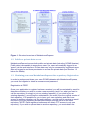
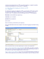


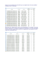
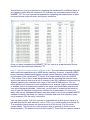


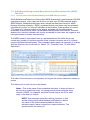

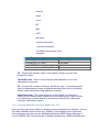
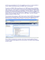


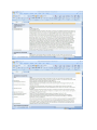
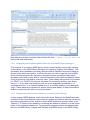

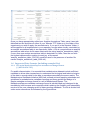


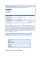

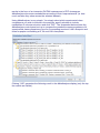


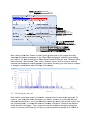
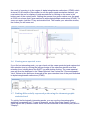


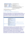


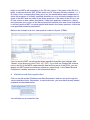
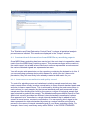


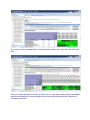


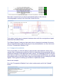
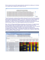
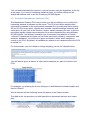

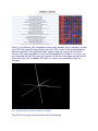
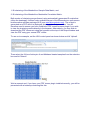
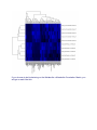

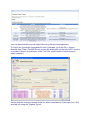

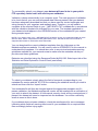

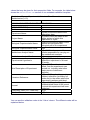


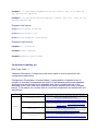
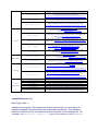


![[U4.52.11] Opérateur NORM_MODE](http://vs1.manualzilla.com/store/data/006367690_1-e7267b98ece1d2d49d0ad0f3eb736201-150x150.png)