
1
User’s Manual of CAIN
Version 2.42
Jun.27.2011
TeXed on June 27, 2011
1
Contents
1 Introduction
1.1 General Structure of Input Data . . . . . . . . . . . . . . . . . . . . . . . .
2 Basic Grammer of the Input Data
2.1 System of Units . . . . . . . . . . .
2.2 Characters . . . . . . . . . . . . . .
2.3 File Lines and Command Blocks . .
2.4 Commands . . . . . . . . . . . . .
2.5 Expressions . . . . . . . . . . . . .
2.5.1 Operators . . . . . . . . . .
2.5.2 Pre-defined parameters . . .
2.5.3 User-defined parameters . .
2.5.4 Predefined functions . . . .
2.5.5 Arrays . . . . . . . . . . . .
2.5.6 Character expression . . . .
2.6 CAIN functions . . . . . . . . . .
2.6.1 Beam statistics functions . .
2.6.2 Test particle functions . . .
2.6.3 Beamline functions . . . . .
2.6.4 Luminosity-related function
2.6.5 Laser-related function . . .
2.6.6 Special functions . . . . . .
2.7 Meta-expression . . . . . . . . . . .
2.8 External Files . . . . . . . . . . . .
.
.
.
.
.
.
.
.
.
.
.
.
.
.
.
.
.
.
.
.
.
.
.
.
.
.
.
.
.
.
.
.
.
.
.
.
.
.
.
.
3 Commands
3.1 ALLOCATE . . . . . . . . . . . . . . . .
3.2 FLAG . . . . . . . . . . . . . . . . . . .
3.3 SET . . . . . . . . . . . . . . . . . . . .
3.4 ARRAY . . . . . . . . . . . . . . . . . .
3.5 BEAM . . . . . . . . . . . . . . . . . . .
3.5.1 Definition by Twiss parameters
3.5.2 Read particle data from a file .
3.5.3 Single particle . . . . . . . . . .
3.5.4 Test particles . . . . . . . . . .
2
.
.
.
.
.
.
.
.
.
.
.
.
.
.
.
.
.
.
.
.
.
.
.
.
.
.
.
.
.
.
.
.
.
.
.
.
.
.
.
.
.
.
.
.
.
.
.
.
.
.
.
.
.
.
.
.
.
.
.
.
.
.
.
.
.
.
.
.
.
.
.
.
.
.
.
.
.
.
.
.
.
.
.
.
.
.
.
.
.
.
.
.
.
.
.
.
.
.
.
.
.
.
.
.
.
.
.
.
.
.
.
.
.
.
.
.
.
.
.
.
.
.
.
.
.
.
.
.
.
.
.
.
.
.
.
.
.
.
.
.
.
.
.
.
.
.
.
.
.
.
.
.
.
.
.
.
.
.
.
.
.
.
.
.
.
.
.
.
.
.
.
.
.
.
.
.
.
.
.
.
.
.
.
.
.
.
.
.
.
.
.
.
.
.
.
.
.
.
.
.
.
.
.
.
.
.
.
.
.
.
.
.
.
.
.
.
.
.
.
.
.
.
.
.
.
.
.
.
.
.
.
.
.
.
.
.
.
.
.
.
.
.
.
.
.
.
.
.
.
.
.
.
.
.
.
.
.
.
.
.
.
.
.
.
.
.
.
.
.
.
.
.
.
.
.
.
.
.
.
.
.
.
.
.
.
.
.
.
.
.
.
.
.
.
.
.
.
.
.
.
.
.
.
.
.
.
.
.
.
.
.
.
.
.
.
.
.
.
.
.
.
.
.
.
.
.
.
.
.
.
.
.
.
.
.
.
.
.
.
.
.
.
.
.
.
.
.
.
.
.
.
.
.
.
.
.
.
.
.
.
.
.
.
.
.
.
.
.
.
.
.
.
.
.
.
.
.
.
.
.
.
.
.
.
.
.
.
.
.
.
.
.
.
.
.
.
.
.
.
.
.
.
.
.
.
.
.
.
.
.
.
.
.
.
.
.
.
.
.
.
.
.
.
.
.
.
.
.
.
.
.
.
.
.
.
.
.
.
.
.
.
.
.
.
.
.
.
.
.
.
.
.
.
.
.
.
.
.
.
.
.
.
.
.
.
.
.
.
.
.
.
.
.
.
.
.
.
.
.
.
.
.
.
.
.
.
.
.
.
.
.
.
.
.
.
.
.
.
.
.
.
.
.
.
.
.
.
.
.
.
.
.
.
.
.
.
.
.
.
.
.
.
.
.
.
.
.
.
.
.
.
.
.
.
.
.
.
.
.
.
.
.
.
.
.
.
.
.
.
.
.
6
7
.
.
.
.
.
.
.
.
.
.
.
.
.
.
.
.
.
.
.
.
10
10
10
10
11
12
13
14
15
15
16
16
18
18
19
20
21
21
21
22
22
.
.
.
.
.
.
.
.
.
24
25
25
26
26
27
27
30
32
33
3.6
3.7
3.8
3.9
3.10
3.11
3.12
3.13
3.14
3.15
3.16
3.17
3.18
3.19
3.20
3.21
3.22
3.23
3.24
3.25
3.26
3.27
3.5.5 Caution . . . . . . . . . . . . . . . . . . . . . .
LASER . . . . . . . . . . . . . . . . . . . . . . . . . . .
3.6.1 General laser parameters . . . . . . . . . . . . .
3.6.2 Time profile parameters . . . . . . . . . . . . .
3.6.3 Spatial profile parameters . . . . . . . . . . . .
3.6.4 File format . . . . . . . . . . . . . . . . . . . .
3.6.5 Laser-related CAIN functions . . . . . . . . . .
LASERQED . . . . . . . . . . . . . . . . . . . . . . . . .
CFQED . . . . . . . . . . . . . . . . . . . . . . . . . . .
BBFIELD . . . . . . . . . . . . . . . . . . . . . . . . . .
EXTERNALFIELD . . . . . . . . . . . . . . . . . . . . . .
LUMINOSITY . . . . . . . . . . . . . . . . . . . . . . . .
PPINT . . . . . . . . . . . . . . . . . . . . . . . . . . .
PUSH, ENDPUSH . . . . . . . . . . . . . . . . . . . . . . .
DRIFT . . . . . . . . . . . . . . . . . . . . . . . . . . .
LORENTZ . . . . . . . . . . . . . . . . . . . . . . . . . .
MAGNET . . . . . . . . . . . . . . . . . . . . . . . . . . .
BEAMLINE . . . . . . . . . . . . . . . . . . . . . . . . .
BLOPTICS . . . . . . . . . . . . . . . . . . . . . . . . .
MATCHING . . . . . . . . . . . . . . . . . . . . . . . . .
TRANSPORT, ENDTRANSPORT . . . . . . . . . . . . . . . .
DO, CYCLE, EXIT, ENDDO . . . . . . . . . . . . . . . . . .
IF, ELSEIF, ELSE, ENDIF . . . . . . . . . . . . . . . . .
WRITE, PRINT . . . . . . . . . . . . . . . . . . . . . . .
3.23.1 Write the macro-particle data . . . . . . . . . .
3.23.2 Write the beam statistics data . . . . . . . . . .
3.23.3 Write the calculated luminosity . . . . . . . . .
3.23.4 Write a list of defined magnets . . . . . . . . . .
3.23.5 Write the beamline optics . . . . . . . . . . . .
3.23.6 Write the beamline geometry . . . . . . . . . .
3.23.7 Write the values of parameters and expressions
3.23.8 Write a list of all allocated arrays . . . . . . . .
3.23.9 Write the cpu time . . . . . . . . . . . . . . . .
PLOT . . . . . . . . . . . . . . . . . . . . . . . . . . . .
3.24.1 Histogram of particle data . . . . . . . . . . . .
3.24.2 Scatter plot of particles or laser photons . . . .
3.24.3 Plot the test particle data . . . . . . . . . . . .
3.24.4 Plot the differential luminosity . . . . . . . . . .
3.24.5 Plot charge distribution and beam-beam field .
3.24.6 Plot beamline optics . . . . . . . . . . . . . . .
3.24.7 Plot beamline geometry . . . . . . . . . . . . .
3.24.8 Plot a function . . . . . . . . . . . . . . . . . .
CLEAR . . . . . . . . . . . . . . . . . . . . . . . . . . .
FILE . . . . . . . . . . . . . . . . . . . . . . . . . . . .
HEADER . . . . . . . . . . . . . . . . . . . . . . . . . . .
3
.
.
.
.
.
.
.
.
.
.
.
.
.
.
.
.
.
.
.
.
.
.
.
.
.
.
.
.
.
.
.
.
.
.
.
.
.
.
.
.
.
.
.
.
.
.
.
.
.
.
.
.
.
.
.
.
.
.
.
.
.
.
.
.
.
.
.
.
.
.
.
.
.
.
.
.
.
.
.
.
.
.
.
.
.
.
.
.
.
.
.
.
.
.
.
.
.
.
.
.
.
.
.
.
.
.
.
.
.
.
.
.
.
.
.
.
.
.
.
.
.
.
.
.
.
.
.
.
.
.
.
.
.
.
.
.
.
.
.
.
.
.
.
.
.
.
.
.
.
.
.
.
.
.
.
.
.
.
.
.
.
.
.
.
.
.
.
.
.
.
.
.
.
.
.
.
.
.
.
.
.
.
.
.
.
.
.
.
.
.
.
.
.
.
.
.
.
.
.
.
.
.
.
.
.
.
.
.
.
.
.
.
.
.
.
.
.
.
.
.
.
.
.
.
.
.
.
.
.
.
.
.
.
.
.
.
.
.
.
.
.
.
.
.
.
.
.
.
.
.
.
.
.
.
.
.
.
.
.
.
.
.
.
.
.
.
.
.
.
.
.
.
.
.
.
.
.
.
.
.
.
.
.
.
.
.
.
.
.
.
.
.
.
.
.
.
.
.
.
.
.
.
.
.
.
.
.
.
.
.
.
.
.
.
.
.
.
.
.
.
.
.
.
.
.
.
.
.
.
.
.
.
.
.
.
.
.
.
.
.
.
.
.
.
.
.
.
.
.
.
.
.
.
.
.
.
.
.
.
.
.
.
.
.
.
.
.
.
.
.
.
.
.
.
.
.
.
.
.
.
.
.
.
.
.
.
.
.
.
.
.
.
.
.
.
.
.
.
.
.
.
.
.
.
.
.
.
.
.
.
.
.
.
.
.
.
.
.
.
.
.
.
.
.
.
.
.
.
.
.
.
.
.
.
.
.
.
.
.
.
.
.
.
.
.
.
.
.
.
.
.
.
.
.
.
.
.
.
.
.
.
.
.
.
.
.
.
.
.
.
.
.
.
.
.
.
.
.
.
.
.
.
.
.
.
.
.
.
.
.
.
.
.
.
.
33
34
35
36
36
37
39
39
42
43
43
44
46
47
48
49
50
51
52
52
55
57
58
58
59
60
60
60
61
61
61
63
63
63
63
65
66
66
67
68
68
69
69
71
71
3.28
3.29
3.30
3.31
3.32
STORE and RESTORE . . . .
DEBUGFLAG . . . . . . . . .
STOP . . . . . . . . . . . .
END . . . . . . . . . . . . .
Particle selection operand
.
.
.
.
.
.
.
.
.
.
.
.
.
.
.
.
.
.
.
.
.
.
.
.
.
.
.
.
.
.
.
.
.
.
.
.
.
.
.
.
.
.
.
.
.
.
.
.
.
.
.
.
.
.
.
.
.
.
.
.
.
.
.
.
.
.
.
.
.
.
.
.
.
.
.
.
.
.
.
.
.
.
.
.
.
.
.
.
.
.
.
.
.
.
.
.
.
.
.
.
.
.
.
.
.
.
.
.
.
.
.
.
.
.
.
.
.
.
.
.
.
.
.
.
.
.
.
.
.
.
.
.
.
.
.
72
73
73
73
73
4 Installation
4.1 UNIX Version . . . . . . . . . . . . . . . . . .
4.1.1 Directory Structure . . . . . . . . . . .
4.1.2 Compilation . . . . . . . . . . . . . . .
4.1.3 Storage Requirements . . . . . . . . .
4.1.4 Run . . . . . . . . . . . . . . . . . . .
4.2 Windows Version . . . . . . . . . . . . . . . .
4.2.1 Installation . . . . . . . . . . . . . . .
4.2.2 Directory Structure . . . . . . . . . . .
4.2.3 Run . . . . . . . . . . . . . . . . . . .
4.2.4 Difference of usage from UNIX version
4.2.5 TopDrawer . . . . . . . . . . . . . . .
.
.
.
.
.
.
.
.
.
.
.
.
.
.
.
.
.
.
.
.
.
.
.
.
.
.
.
.
.
.
.
.
.
.
.
.
.
.
.
.
.
.
.
.
.
.
.
.
.
.
.
.
.
.
.
.
.
.
.
.
.
.
.
.
.
.
.
.
.
.
.
.
.
.
.
.
.
.
.
.
.
.
.
.
.
.
.
.
.
.
.
.
.
.
.
.
.
.
.
.
.
.
.
.
.
.
.
.
.
.
.
.
.
.
.
.
.
.
.
.
.
.
.
.
.
.
.
.
.
.
.
.
.
.
.
.
.
.
.
.
.
.
.
.
.
.
.
.
.
.
.
.
.
.
.
.
.
.
.
.
.
.
.
.
.
.
.
.
.
.
.
.
.
.
.
.
75
75
75
75
77
77
78
78
78
78
78
79
.
.
.
.
.
.
.
.
.
.
.
.
.
.
.
.
.
.
.
.
.
.
.
.
.
80
80
80
80
81
85
86
87
88
89
89
89
90
92
92
92
93
95
98
98
102
105
109
112
112
113
5 Physics and Numerical Methods
5.1 Coordinate . . . . . . . . . . . . . . . . . . . . . . . . . . . .
5.2 Particle Variables . . . . . . . . . . . . . . . . . . . . . . . .
5.2.1 Arrays for Particles . . . . . . . . . . . . . . . . . . .
5.2.2 Description of Polarization . . . . . . . . . . . . . . .
5.3 Beam Parameters . . . . . . . . . . . . . . . . . . . . . . . .
5.4 Solving Equation of Motion . . . . . . . . . . . . . . . . . .
5.4.1 Equation of motion under DRIFT EXTERNAL command
5.4.2 Equation of motion under PUSH command . . . . . .
5.5 Beamline . . . . . . . . . . . . . . . . . . . . . . . . . . . . .
5.5.1 Beamline Coordinate . . . . . . . . . . . . . . . . . .
5.5.2 Beamline coordinate . . . . . . . . . . . . . . . . . .
5.5.3 Dipole Magnets . . . . . . . . . . . . . . . . . . . . .
5.5.4 Quadrupole Magnets . . . . . . . . . . . . . . . . . .
5.6 Luminosity . . . . . . . . . . . . . . . . . . . . . . . . . . .
5.6.1 Luminosity Integration Algorithm . . . . . . . . . . .
5.6.2 Polarization . . . . . . . . . . . . . . . . . . . . . . .
5.7 Beam Field . . . . . . . . . . . . . . . . . . . . . . . . . . .
5.8 Laser . . . . . . . . . . . . . . . . . . . . . . . . . . . . . . .
5.8.1 Laser Geometry . . . . . . . . . . . . . . . . . . . . .
5.8.2 Linear Compton Scattering . . . . . . . . . . . . . .
5.8.3 Compton Process in a Strong Laser Field . . . . . . .
5.8.4 Breit-Wheeler Process in a Strong Laser Field . . . .
5.9 Beamstrahlung . . . . . . . . . . . . . . . . . . . . . . . . .
5.9.1 Basic formulas . . . . . . . . . . . . . . . . . . . . . .
5.9.2 Algorithm of event generation . . . . . . . . . . . . .
4
.
.
.
.
.
.
.
.
.
.
.
.
.
.
.
.
.
.
.
.
.
.
.
.
.
.
.
.
.
.
.
.
.
.
.
.
.
.
.
.
.
.
.
.
.
.
.
.
.
.
.
.
.
.
.
.
.
.
.
.
.
.
.
.
.
.
.
.
.
.
.
.
.
.
.
.
.
.
.
.
.
.
.
.
.
.
.
.
.
.
.
.
.
.
.
.
.
.
.
.
.
.
.
.
.
.
.
.
.
.
.
.
.
.
.
.
.
.
.
.
.
.
.
.
.
.
.
.
.
.
.
.
.
.
.
.
.
.
.
.
.
.
.
.
.
.
.
.
.
.
.
.
.
.
.
.
.
.
.
.
.
.
.
.
.
.
.
.
.
.
.
.
.
.
.
5.9.3 Polarization . . . . . . . . . . . . . . . . . .
5.9.4 Enhancement factor of the event rate . . . .
5.10 Coherent Pair Creation . . . . . . . . . . . . . . . .
5.10.1 Basic formulas . . . . . . . . . . . . . . . . .
5.10.2 Algorithm of event generation . . . . . . . .
5.11 Incoherent Processes . . . . . . . . . . . . . . . . .
5.11.1 Breit-Wheeler Process . . . . . . . . . . . .
5.11.2 Virtual (almost real) photon approximation
5.11.3 Numerical methods . . . . . . . . . . . . . .
A History of Revision
A.1 CAIN2.42 . . . . . . . . . . . . . . .
A.2 CAIN2.40 . . . . . . . . . . . . . . .
A.3 CAIN2.35 . . . . . . . . . . . . . . .
A.4 CAIN2.33 . . . . . . . . . . . . . . .
A.5 CAIN2.32 . . . . . . . . . . . . . . .
A.6 CAIN2.31 . . . . . . . . . . . . . . .
A.7 CAIN2.3 . . . . . . . . . . . . . . .
A.8 CAIN2.23 . . . . . . . . . . . . . . .
A.9 CAIN2.21 . . . . . . . . . . . . . . .
A.10 CAIN2.2a . . . . . . . . . . . . . . .
A.11 CAIN2.2 . . . . . . . . . . . . . . .
A.12 History until the version CAIN2.1b .
5
.
.
.
.
.
.
.
.
.
.
.
.
.
.
.
.
.
.
.
.
.
.
.
.
.
.
.
.
.
.
.
.
.
.
.
.
.
.
.
.
.
.
.
.
.
.
.
.
.
.
.
.
.
.
.
.
.
.
.
.
.
.
.
.
.
.
.
.
.
.
.
.
.
.
.
.
.
.
.
.
.
.
.
.
.
.
.
.
.
.
.
.
.
.
.
.
.
.
.
.
.
.
.
.
.
.
.
.
.
.
.
.
.
.
.
.
.
.
.
.
.
.
.
.
.
.
.
.
.
.
.
.
.
.
.
.
.
.
.
.
.
.
.
.
.
.
.
.
.
.
.
.
.
.
.
.
.
.
.
.
.
.
.
.
.
.
.
.
.
.
.
.
.
.
.
.
.
.
.
.
.
.
.
.
.
.
.
.
.
.
.
.
.
.
.
.
.
.
.
.
.
.
.
.
.
.
.
.
.
.
.
.
.
.
.
.
.
.
.
.
.
.
.
.
.
.
.
.
.
.
.
.
.
.
.
.
.
.
.
.
.
.
.
.
.
.
.
.
.
.
.
.
.
.
.
.
.
.
.
.
.
.
.
.
.
.
.
.
.
.
.
.
.
.
.
.
.
.
.
.
.
.
.
.
.
.
.
.
.
.
.
.
.
.
.
.
.
.
.
.
.
.
.
.
.
.
.
.
.
.
.
.
.
.
.
.
.
.
.
.
.
.
.
.
.
.
.
.
.
.
.
.
.
.
.
.
.
.
.
.
.
.
.
.
.
114
116
116
116
117
119
120
122
123
.
.
.
.
.
.
.
.
.
.
.
.
126
. 126
. 126
. 126
. 127
. 128
. 128
. 128
. 129
. 129
. 129
. 130
. 130
Chapter 1
Introduction
CAIN is a stand-alone FORTRAN Monte-Carlo code for the interaction involving high
energy electron, positron, and photons. Originally, it started with the name ABEL[1]
in 1984 for the beam-beam interaction in e+ e− linear colliders. At that time the main
concern was the beam deformation due to the Coulomb field and the synchrotron radiation (beamstrahlung). Later, the pair creation by particle-particle collision was added,
and, it was renamed to CAIN when the interaction with laser beams (radiation by electrons/positrons and pair creation by photons in a strong laser field) was added for the
γ-γ colliders.
CAIN home page is located at http://www-acc-theory.kek.jp/members/cain/
The first version CAIN1.1[2], which was a combined program of modified ABEL and
a laser QED code, was limited because it could not handle the laser interaction and the
e+ e− interaction simultaneously and does not accept mixed e+ e− beams. To overcome
these problems, CAIN2.0 was written from scratch. It now allows any mixture of e− , e+ ,
γ and lasers, and multiple-stage interactions. The input data format has been refreshed
completely.
The physical objects which appear in the present version CAIN2.42 are particle
beams, lasers, external fields and magnetic beamlines. The beams may consist of highenergy electrons, positrons and photons.
The direction of the beams is arbitrary but when the Coulomb field is to be calculated
for two colliding beams, a basic assumption is that each beam must be a ‘beam’, i.e., most
particles in each beam go almost parallel. (CAIN assumes the two beams go opposite
direction, right-going and left-going. For the case they make a large angle, you can apply
CAIN command for Lorentz transformation so that the collision looks head-on.)
The lasers can go any direction. As external fields the present version accepts only
constant fields, but since CAIN2.23 you can track a beam though a beamline consisting
of magnets.
The physical processes that can be handled by the present version CAIN2.42 are
• Classical interaction (orbit deformation) due to the Coulomb field.
• Luminosity between beams (e− e+ γ).
• Synchrotron radiation by electrons/positrons (beamstrahlung), and pair creation by
high energy photons (coherent pair creation) due to the beam field.
6
• Interaction of high energy photon or electron/positron beams with laser field, including the nonlinear effects of the field strength.
• Classical and quantum interactions with a constant external field.
• Incoherent e+ e− pair creation by photons, electrons and positrons.
• Transport of charged particles through a magnetic beamline.
• In almost all interactions the polarization effects can be included.
Output data (properties of particles, luminosities, etc.) can be written in specified
files at any moment of job. The graphic output is written only in the TopDrawer format.
If you want other formats, you have to write a post processor by yourself.
1.1
General Structure of Input Data
In this section we briefly describe the structure of input data. CAIN is not intended for
interactive jobs because the computing time is normally more than several minutes. Every
instruction to the program is given in the input data. Two cases, a simple e+ e− collision
and a γ-γ collider, are given here as examples. For more detail look at the sections for
each command and the example input data files in the directory cain242/in.
Consider a simple e+ e− collision. You have first to define the two beams:
BEAM
RIGHT, KIND=2, NP=10000, AN=1E10, E0=500E9, SIGT=1E-4,
BETA=(1E-2,1E-4), EMIT=(3E-12,3E-14);
This defines a right-going electron (KIND=2) beam with the bunch population 1 × 10¹⁰ ,
energy 500GeV, bunch length 100µm, etc. Note that every command must end with a
semicolon.
You can use variables and mathematical expressions (see Sec.2.5). For example, if you
prefer normalized emittance, you may write
SET
ee=500E9, gamma=ee/Emass, emitx=3D-6/gamma, emity=3D-8/gamma,
betax=1E-2, betay=1E-4,
sigx=Sqrt(emitx*betax), sigy=Sqrt(emity*betay);
BEAM RIGHT, KIND=2, NP=10000, AN=1E10, E0=ee, SIGT=1E-4,
BETA=(betax,betay), EMIT=(emitx,emity);
Emass is a reserved variable and Sqrt is a predefined function. sigx and sigy are defined
for later use. If you like millimeter instead of meter, you may say
SET
BEAM
mm=1E-3, sigz=0.1*mm;
........ SIGT=sigz, ......;
Now you know how to define the positron (KIND=3) beam. Obviously, BEAM LEFT,
KIND=3, . . .; will do.
For calculating the beam-beam force you need to tell CAIN about the mesh:
SET Smesh=sigz/2;
BBFIELD NX=32, NY=32, WX=8*sigx, R=sigx/sigy/2;
7
The definition of the longitudinal mesh Smesh may look bizzarre. This is because the
same mesh is used for luminosity calculation.
For computing the e+ e− luminosity, you have to say, for example,
LUMINOSITY KIND=(2,3), W=(0,2*ee,50), WX=8*sigx, WY=8*sigy, FREP=90*150;
if the rep rate is 90 bunches times 150Hz. WX and WY define the mesh region (See Sec.3.11).
Now you are ready to start the collision.
FLAG OFF ECHO;
PUSH Time=(-2.5*sigz,2.5*sigz,200);
ENDPUSH;
will track the beam over the specified time range in 200 steps. It is better to turn off the
echo before running. You can get the transient information (e.g., plot the beam profile
during collision) by inserting commands (PLOT, WRITE etc) between PUSH and ENDPUSH.
If you want the beamstrahlung, you have to insert
CFQED
BEAMSTRAHLUNG;
before PUSH. After ENDPUSH you can plot (generate TopDrawer input file) the e+ e− differential luminosity by
PLOT LUMINOSITY, KIND=(2,3);
You can also plot particle distribution. For example, for plotting the photon (KIND=1)
energy spectrum,
PLOT
HIST, KIND=1, H=En/1E9, HSCALE=(0,ee/1E9,50),
TITLE=’Beamstrahlung Energy Spectrum;’,
HTITLE=’E0G1 (GeV); XGX
;’;
H defines the horizontal axis (energy in units of GeV, in this example). Unfortunately,
the present version creates input data for TopDrawer only.
You may want different outputs without repeating the time-consuming calculation.
You can do the following. After ENDPUSH, store all the variables and the particle data:
STORE FILE=’aaa’;
WRITE BEAM, FILE=’bbb’;
and restore them in the input file for the next job
RESTORE FILE=’aaa’;
BEAM FILE=’bbb’;
PLOT ........;
γ-γ collider is more complex. Three steps, e-γ conversion of right-going electron,
that of left-going electron, and γ-γ collision, are needed. You can do these steps in one
job or in separate jobs using STORE/WRITE and RESTORE/BEAM FILE commands. The
attached example cain242/in/NLCggCP.i executes the two conversions and NLCggIP.i
the collision at the interaction point.
For the conversion you define the lasers in addition to the initial electron beam:
8
LASER LEFT, WAVEL=laserwl, POWERD=powerd,
TXYS=(-dcp,0,off/2,-dcp),
E3=(0,-Sin(angle),-Cos(angle)), E1=(1,0,0),
RAYLEIGH=(rlx,rly), SIGT=sigt, STOKES=(0,1,0) ;
See Sec.3.6 for the meaning of the key words. The type of laser-electron and laser-γ
interactions has to be specified by LASERQED command:
LASERQED
LASERQED
COMPTON, NPH=5, XIMAX=1.1*xi, LAMBDAMAX=1.1*lambda ;
BREITW, NPH=5, XIMAX=1.1*xi, ETAMAX=1.1*eta ;
The PUSH-ENDPUSH loop is the same as in the e+ e− example.
After ENDPUSH write all the particle data by WRITE BEAM, FILE=... or, if you do not
want to include e-e collision, write the photon data selectively by WRITE BEAM, KIND=1,
FILE=. . .. Then, read this file in the next job and simulate the γ-γ collision.
See Sec.2 for the basic grammer of the input data. See Sec.2.4 for a list of all the
available commands.
9
Chapter 2
Basic Grammer of the Input Data
2.1
System of Units
MKSA is used throughout. The particle energy and momentum are eV and eV/c, respectively. An exception is the luminosity which is expressed in cm−2 sec−1 . The time (e.g.,
the laser pulse length, time coordinate of particles, etc.) is always expressed in units of
meter by multiplying the velocity of light.
2.2
Characters
Upper and lower case alphabets are distinguished. The following characters have special
use:
= ; , ( [ { ) ] } ! ’ "
Also, the following characters are used in mathematical expressions:
+ - * / ^ = < > & $ | . : ( [ { ) ] }
The command names and (almost all) keywords consist of upper case alphabets only.
Variables may consist of upper/lower case alphabets, numerical characters and underscore
‘ ’.
2.3
File Lines and Command Blocks
The input data is a collection of file lines. Upto 256 characters in a line are read in.
(This limitation can be easily changed by modifying the parameter statement in the main
program.)
A literal character string is defined as a string enclosed by a pair either of apostrophes
’ or of double apostrophes ". (See Sec.2.5.6 for more detail.) The string must close within
a file line.
If a character “!” is encountered, the whole text after it to the end of the file line is
considered as a comment, unless the “!” is in a literal character string.
Apart from the above two points (i.e, that a character string must close within a
file line and that “!” is effective till the end of the file line), the concept of ‘file line’ is
irrelevant. Therefore, for example, continuing the two file lines will give the same results,
10
1
and the end of a command must explicitly stated (by semicolon “;”) without relying on
the end-of-line.
The whole text, after the comment part is eliminated, is divided into ‘command blocks’.
The end of a command block is indicated by a semicolon “;” if the “;” is not in a literal
character string.
Each command block has the following structure:
command name
operand, operand, · · · operand ;
After the command name before the first operand, there must be at least one blanck
character (unless there is no operand). Operands are separated by a comma “,” and the
number of blancks before and after “,” is arbitrary. (In some commands, “,” can be
replaced by one or more blancks). Unless stated in each command description in the next
section, the order of operands is arbitrary.
An operand is either a single keyword (a flag) or of the form
keyword = right hand side
A keyword is an alphanumerical string predefined for each command. The right hand side
is just a number or an ‘expression’ (to be explained later) or of the form
( expression, expression, · · · expression)
The parenthesis ( ) may be replaced by [ ] or { } if they match. In the case when all the
expressions are expected to be floatng type (i.e., not character type), the right-hand-side
can be replaced by an array name without subscripts. It must be a one-dimensional array
and its full size is used. For example,
ARRAY a(2); SET a(1)=2, a(2)=3;
command keyword=a;
is equivalent to
command keyword=(2,3);
2.4
Commands
As stated above, each command block must start with a command name. The present
version has the following commands
ALLOCATE
Memory allocation for big arrays. Sec.3.1.
FLAG
On-off flags (echo, etc.). Sec.3.2.
SET
Define user variables. Sec.3.3.
ARRAY
Allocate array variables, Sec.3.4.
BEAM
Define particle beams. Sec.3.5.
LASER
Define lasers. Sec.3.6.
EXTERNALFIELD Define external (static) electromagnetic field. Sec.3.10.
LASERQED
Parameters for the laser-particle interaction. Sec.3.7.
1
Here is some problem since blanck characters in a line after the last non-blanck character are ignored.
For example, SET / x=0 (/ is line feed) is understood as SETx=0 even if there is a blanck character following
SET.
11
CFQED
Parameters for the interaction between particles and constant electromagnetic field (beamstrahlung and coherent pair creation). Sec.3.8.
BBFIELD
Method of calculation of the beam field. Sec.3.9.
PPINT
Incoherent particle-particle interaction. Sec.3.12.
LUMINOSITY
Define what sort of luminosities to be calculated. Sec.3.11.
LORENTZ
Lorentz transformation. Sec.3.15.
MAGNET
Define a magnet for beamline transportation. Sec.3.16.
BEAMLINE
Define configuration of a beamline. Sec.3.17.
MATCHING
Optics matching of a beamline. Sec.3.19.
BLOPTICS
Calculate Twiss parameters of a beamline. Sec.3.18
TRANSPORT,ENDTRANSPORT Loop for beam transportation along a beamline. Sec.3.20
DRIFT
Move particles in vaccuum or in external field. Sec.3.14.
PUSH,ENDPUSH
Loop of time steps. Sec.3.13.
DO,CYCLE,EXIT,ENDDO Do loop. Sec.3.21.
IF,ELSEIFELSE,ENDIF If block. Sec.3.22.
WRITE,PRINT
Print on screen or on a file. Sec.3.23.
PLOT
Plot using TopDrawer. Sec.3.24.
CLEAR
Clear data or disable commands. Sec.3.25.
FILE
Open/close files. Sec.3.26.
HEADER
Define the header for graphic outputs. Sec.3.27.
STORE,RESTORE
Save/recall variables and luminosity values. Sec.3.28.
STOP
Stop run. Sec.3.30.
END
End of the input file. Sec.3.31.
The command names may be shortened if not ambiguous. Therefore, LASERQ is equivalent to LASERQED. This rule applies also to the operand keywords of all commands. (But
does not apply to parameter and function names.)
2.5
Expressions
In the example in Sec.1.1, the right hand sides of some operands are written in the form
of mathematical expressions. In general, it may contain
• Literal numbers, such as 2, 2.0, -3E-5, etc.
To indicate the exponent, any of E,e,D,d,Q,q may be used. Note that there is no
integer expression so that 2 is identical to 2.0.
• Literal character string enclosed by a pair of apostrophes ’ or of double apostrophes
".
12
• Arithmetic operators +,-,*,/,^.
• Relational operators ==, <, >, <=, >=, =<, =>, <>, ><, /=.
• Logical operators &&, ||.
• Parenthesis: ( [ { ) ] } . Must match.
• Parameters (variables). They are classified as scalar and array or as pre-defined and
user-defined or floating and character string. There is no pre-defined array as of
Cain2.3.
• Functions (pre-defined only).
The result of an expression is either a double-precision floating value or a character string.
There is no integer type expression. Expressions involving character strings will be described later (Sec.2.5.6).
2.5.1
Operators
Arithmetic operators
As arithmetic operators you can use +, -, *, /, ^. Note that power is indicated by “^”
instead of “**” of FORTRAN.
Relational operators
Too many operators are defined: ==, <, >, <=, >=, =<, =>, <>, ><, /=. Among these, the
members of each of the group (<=, =<), (>=,=>), and (<>, ><, /=) have the same meaning.
Results of operation are either 0.0 (false) or 1.0 (true). Thus, for example, 2*(x>=y)-1
is 1 if x ≥ y and is −1 if x < y.
Note, CAIN does not have integer type variables so that, for example, the result of
SET x=1/5, y=(5*x>=1); is unpredictable. Nevertheless, an integral number in floating
format does not have fractional part unless the number of digits exceeds the double
precision limit (about 15 digits). Therefore, SET x=3, y=5, z=(x+2>=y); still works as
you intend.
Logical operators
In a logical expression a && (or ||) b, any number is treated as false if zero and as true
if nonzero. The result of operation is either 0.0 (false) or 1.0 (true).
Priority of operators
The priority of the operators is as follows:
^, (*, /), (+, -), (<, >, <=, >=), (==, <>), &&, ||.
The operators within a pair of braces have the same priority. In contrast to the C language,
the substitution = is not treated as an operator. (It would cause a confusion with our
command syntax keyword=operator, which is not an expression as a whole.)
13
2.5.2
Pre-defined parameters
There are three types of predefined parameters.
• The first type is the universal constants that never change:
Pi
E
Euler
Deg
Cvel
Hbar
Hbarc
Emass
Echarge
Reclass
LambdaC
FinStrC
π
e = 2.718 . . .
Euler’s constant γE = 0.577 . . .
π/180 = 0.0174. . .. You can write, e.g., 10*Deg where the randian
unit is required.
Velocity of light (m/sec).
Planck’s constant (Joule·sec).
Planck’s constant times the velocity of light (eV·m).
Electron mass (eV/c2 ).
Elementary charge (Coulomb).
Classical electron radius (m).
Compton wavelength (m).
Fine structure constant.
• The second type is the parameters whose values are determined by the program.
Users cannot change their values but can refer to. These variables have definte
meanings only under certain situations. For example, Time makes sense in the
PUSH-ENDPUSH loop, $PrevMag in the TRANSPORT-ENDTRANSPORT loop, etc. Those
from T to Incp refer to each particle and, therefore, have definte meanings only in
loop statements over particles (for example, in defining the axes for plots).
Time
Running variables for global time coordinate (m). Makes sense only
inside PUSH-ENDPUSH loop.
T,X,Y,S
Running variables for particle coordinate (m).
En,Px,Py,Ps Running variables for energy-momentum (eV, eV/c). The energy
is En but not E.
Sx,Sy,Ss
Electron/positron spin. Helicity may be written approximately as
Ss*Sgn(Ps).
Xi1,Xi2,Xi3 Photon Stokes parameters ξ1 , ξ2 , ξ3 .
Kind
Particle species. 1,2,3 for photon, electron, positron.
Gen
Particle generation.
Wgt
Particle weight. (One macro-particle represents Wgt real particles.
Incp
1 if the particle is created by an incoherent process. Otherwise 0.
$PName
Particle name. 4 bytes. Normally blanck. The first character is
‘T’ for test particles, ‘I’ for incoherent particles. ‘IBW ’, ‘IBH ’,
‘ILL ’, ‘IBR ’ for incoherent particles created by Breit-Wheeler,
Bethe-Heitler, Landau-Lifshitz, Bremsstrahlung processes, respectively. ‘LOST’ for lost particles.
14
Ln,Lij
(n=0,1,2,3,4, i,j=0,1,2,3) Luminosity values used in PLOT LUMINOSITY
command.
W
Center-of-mass energy used in PLOT LUMINOSITY command.
Sbl
s-coordinate in a beamline. Makes sense only inside TRANSPORTENDTRANSPORT loop.
$PrevMag Character. Name of the previous magnet. Valid only during a
TRANSPORT-ENDTRANSPORT loop.
$NextMag Character. Name of the next magnet. Valid only during a TRANSPORTENDTRANSPORT loop.
$InFilePath Full path of the input file directory. (includes the last character
‘/’ (UNIX) or ‘\’ (Windows)).
$InFileName Name of the input file (without path, with extension).
• The third type is those whose names are predefined with default values and which
the user can change (by SET command) such as
MsgFile
OutFile
OutFile2
TDFile
MsgLevel
Rand
Debug
Smesh
2.5.3
File reference number for echo, error messages, and default destination of PRINT command. (default=6)2
File reference number for voluminous outputs. The default destination of WRITE command. (default=12)
Other print output. Not used. (default=12)
TopDrawer file number. (default=8)
Message level. (default=0, i.e., error messages only)
Random number seed. Positive odd integer other than 1, default=3.
You can reset random number at any time.
Debug parameter for the programmer. If you set Debug≥2, call and
return from major subroutines are announced. (default=0)
Longitudinal mesh size (m) for the calculation of beam-beam field,
luminosity, etc. No default value.
User-defined parameters
These are those defined by SET command. (see Sec.3.3) Upto 16 characters consisting of
upper/lower case alphabets, numericals, and underscore ‘_’. The first character must not
be a numerical. The first character of character type variables must be ‘$’ (and no ‘$’ in
the body).
2.5.4
Predefined functions
There are following basic math functions.
Int,Nint,Sgn,Step,Abs,Frac,Sqrt,Exp,Log,Log10,
2
The input file number is set to 5. If you want to change it, see the variable RDFL in the file
’cain242/src/initlz.f’.
15
Cos,Sin,Tan, ArcSin,ArcCos,ArcTan,
Cosh,Sinh,Tanh, ArcCosh,ArcSinh,ArcTanh, Gamma,
Mod, Atan2, Min, Max
Defintions are the same as in standard FORTRAN except Sgn and Step:
1
(
for x > 0
for x = 0
Sgn(x) = 0
−1 for x < 0
Step(x) =
1 for x ≥ 0
0 for x = 0
Enclose the argument by ( ) or [ ] or { }. Separate arguments by “,” if there are more
than one argument (Mod, Atan2, Min, Max). (Number of arguments for Min and Max is
arbitrary.)
In addition to the above functions of standard type there are functions of other type,
which are defined for CAIN. See the next subsection Sec.2.6.
2.5.5
Arrays
You can allocate (or deallocate) arrays by using the command ARRAY and set their values
by SET command. The rule about the array name is the same as that of user-defined
parameters. The subscripts are delimited by commas and enclosed by a pair of parenthesis
( ) or [ ] or { }(must match). For example,
ARRAY
SET
ARRAY
a(20,0:10);
a(3,4)=5.0,
FREE a;
x=a(3,4);
When the lower bound of a subscript is not specified in ARRAY command, 1 is assumed as
in FORTRAN. Total number of arrays and the maximum rank is limited (but reasonably
large number) by FORTRAN parameter statement but the size of each array is arbitrary
as long as your computer memory allows. See Sec.3.4 for more detail.
2.5.6
Character expression
A literal character string is defined as a string enclosed by a pair either of apostrophes ’
or of double apostrophes ". The string must close within a file line.3 When you need a
long string, you can use concatenation like ’abc’ + ’xyz’ to be explained below.
Within a string enclosed by ’ (") you can use " (’) as a normal character. The
FORTRAN rule that two successive ’ or " are recognized as a single ’ or " is still valid
but not reccommended (there can be bugs). Even if you have both ’ and " in a string,
you can write like "’"+’"’.
Character expressions have been introduced since CAIN2.3. All expressions can be
classified into two types, floating and character, according to the results.
3
When a file line is read from a file, blanck spaces to the end of the line cause a problem. There is
no way in standard FORTRAN to distinguish between blanck spaces existing in the file and those added
when read in.
16
A variable with the first character $ (up to 16 characters including the $, no $ in the
body) is treated as a character string variable. For example,
SET $a = ’abc’, $b=$a + ’xyz’;
will define $b as a string containing ’abcxyz’. Basically, when an operand of a command
is of the form keyword=’something’ such as file names, you can use a general form of
character expression including character variables for the right-hand-side.4 For example,
SET $fn=’abc’, n=3;
FILE OPEN, UNIT=20, NAME=$fn+$ItoA(n)+’.txt’;
opens a file with the name ’abc3.txt’. (See below for $ItoA.)
There are various limits for the size of character stack (e.g., total number of variable
names, total stored number of characters, total number of characters in one expression,
etc). They cannot be changed by the ALLOCATE command, basically because FORTRAN90
does not allow dynamic allocation of a character string of dynamically determined length.
However, the prepared sizes are large enough for normal uses.
The only possible operations involving character strings are
• Concatenation by +. The result is a character string.
• Multiplication by a positive integer like, e.g., 2*$a (or $a*2) which is equivalent to
$a+$a. The result is a character string.
• Relational operation like $a==$b. The result is a floating number either 0.0 or 1.0.
The result of $a>$b may depend on the platform (lexical order or ascii code order).
Note that due to the standard FORTRAN rule the result of $a==$b is true (1.0)
when $a=’abc’ and $b=’abc ’.
You can introduce arrays of character strings in the same way as floating numbers, e.g.,
by
ARRAY
$a(3,0:5);
This only defines a pointer. Strings are actually allocated when defined by SET command.
The elements of an array may have different lengths.
There are a few functions related to character strings. Obviously, when the first
character of the function name is $, it returns a character string, otherwise a floating
number.
Strlen
Length of a character string, e.g.,
SET n=Strlen($a);
AtoF
Convert a character string into a floating number, e.g.,
SET $a=’1e10’, x = AtoF($a);
4
However, when this manual says ’apostrophes can be omitted’, such as the case of magnet names,
you cannot use the general form. You have to use the name alone or the name enclosed by apostrophes.
17
$FtoA
Convert a floating number into a character string. A format must be
specified like
SET $a=$FtoA(5.3,’(F4.2)’);
which will define a string $a=’5.30’. ( ) will be added when the format
string is not enclosed by ( ).
$ItoA
Convert a floating number into a character string after operating Nint.
For example,
SET $a=$ItoA(3.2);
will create a string $a=’3’. You can optionally specify the format like
SET $a=$ItoA(4.2,’(I3.3)’);
which results in $a=’004’. (Consult your FORTRAN manual.) ( ) will
be added when the format string is not enclosed by ( ).
$Substr
Substring. $Substr($a,n1 ,n2 ) is the substring of $a from n1 -th character (start from 1) to n2 -th character. If n2 is omitted, the end of $a is
used. A null string is returned if n2 < n1 .
Strstr
Strstr($a,$b) searches for the first occurence of the string $b within
the string $a and return the position of the first character (start from 1)
if found. Return 0.0 if not found or if illegal (zero length of $b etc).
$ToUpper
Get a string with all lower case characters converted to upper case.
SET $b=$ToUpper($a);
$ToLower
Get a string with all upper case characters converted to lower case.
2.6
CAIN functions
In addition to the predefined functions of general use, such as Sin and Cos, there are
other special functions intrinsic to CAIN. They are:
Beam statistics functions
Average/rms quantities of the beam such as SigX.
Test particle functions
Retrieves parameters of individual test particles.
Beamline functions
Twiss parameters, etc.
Luminosity-related functions
Retrieves luminosity
Laser-related functions
Local laser intensity, etc.
Special functions
Such as Bessel functions.
2.6.1
Beam statistics functions
The number of particles, that of macro particles, the average coordinates/energy-momentum/polarization
and their r.m.s. values of the beam at the given moment are retrieved by
NParticle, NMacro,
AvrT, AvrX, AvrY, AvrS, SigT, SigX, SigY, SigS,
AvrEn, AvrPx, AvrPy, AvrPs, SigEn, SigPx, SigPy, SigPs,
18
AvrSx,AvrSy,AvrSs,AvrXi1,AvrXi2,AvrXi3,
SigSx,SigSy,SigSs,SigXi1,SigXi2,SigXi3,
BeamMatrix
The calling sequence is common to these functions except BeamMatrix. Let us take SigX
as an example.
SigX(j,k) (j= 1 or 2 or 3, k= 1 or 2 or 3)
returns the horizontal r.m.s. size of right-going (j=1) or left-going (j=2) or both (j=3)
of the photon (k=1) or electron (k=2) or positron (k=3) beam. The particles created
by incoherent processes are excluded. (See below for how to include them.)
There can be one more argument,5 which must be enclosed by a pair of apostrophes (a
character expression in general), like
SigX(j,k,’f ’)
where f is a logical expression for selecting particles. It may contain variables of individual particles (such as En, X, etc). Then, the particles that make f true (i.e., 6=0) are
selected. For example,
SigX(1,2,’En>1e9 && En<2e9’)
will select right-going electrons with energy between 1 and 2 GeV. (See Sec.3.32 for more
detail.) The reason that f must be enclosed by apostrophes is that f must not be evaluated immediately but is to be evaluated later individually for each particle.
When the particle selection argument is given, the incoherent particles are
included by default. If you want to exclude them, you should say, e.g.,
SigX(1,2,’En>1e9 && En<2e9 && Incp==0’)
When you include incoherent particles only, you should of course say Incp==1.
The variables (Sx,Sy,Ss) are used for the spin of electrons/positrons and those (Xi1,Xi2,Xi3)
for polarization of photons. However, these two sets are not actually distinguished. For
example, AvrSs(1,2) means average electron helicity but it is equivalent to AvrXi3(1,2).
BeamMatrix requires two more arguments
BeamMatrix(a,b,j,k,’f ’) (1≤a,b≤8)
The returned value is the average of xa xb where xa =(T,X,Y,S,En,Px,Py,Ps) for a=1 to 8.
(In units of m and eV or eV/c.)
2.6.2
Test particle functions
The coordinates and the energy momentum of the test particles can be retrieved by the
functions
TestT, TestX, TestY, TestS, TestEn, TestPx, TestPy, TestPs
The calling sequence is, for example, TestX(’name’) or TestX(n), where ’name’ is
the character string for the particle name and n is an expression representing an integer
−99 ≤ n ≤ 999. (See Sec.3.5 for the test particle name.)
5
The meaning of this argument has changed since CAIN2.3. It used to be selecting the range of S
coordinate but has been replaced by a more powerful one.
19
2.6.3
Beamline functions
The functions related to the beamline optics such as β and η functions and the transfer
matrix are retrieved by
Beta, Alpha, Eta, Etaprime, Nu, TMat
(Nu is the phase advance /(2π) from the beamline entrance. TMat is the 6×6 linear
transfer matrix from the beamline entrance.) Prior to use, you must compute the optics
by BLOPTICS command. The calling sequence of these functions are the same except for
TMat:
Beta(j, mag , ’bl name’)
where
j
1 or 2 for x or y, respectively.
mag
Either integer or character expression. If it is an integer n > 0, the exit of
the n-th magnet in the beamline is implied. (Beamline entrance if n ≤ 0
and beamline exit if n is equal to or larger than the number of magnets in
the beamline.)
If mag is a character expression, it is identified as a magnet name. If there
are more one magnets with the same name, you can add the occurence
number after a dot. For example, the exit of the third QF is ’QF.3’. You
can of course write as ’QF.’+$ItoA(3). If omitted, the first occurence is
assumed. If you forget apostrophes and write Beta(1,QF,’blname’), you
will get an error message like ‘Variable QF not found’.
bl name
Beamline name. Must be enclosed by apostrophes. (character expression in
general)
You can omit the third argument if in a TRANSPORT-ENDTRANSPORT loop. The default is
the current beam line. (Even in this case you have to call BLOPTICS command prior to
TRANSPORT. Note that Twiss parameters are not needed for particle tracking.) You can
also omit the second argument, which means the current position.
You can omit the third argument during optics matching (i.e., in the matching condition), but cannot omit the second argument in this case.
These functions return zero when an error occurs (such as BLOPTICS not called, the
beamline not existing, illegal number after the dot, etc.).
The calling sequence of TMat is
TMat(i,j, mag , ’bl name’)
where
i,j
1 ≤ i, j ≤ 6. Identify the matrix element.
mag, bl name Same as Twiss parameters.
caution: The 5th column/row of the transfer matrix corresponds to the time variable
(multiplied by the velocity of linght). It is negative at the bunch head, because the head
comes to a given machine point earlier. The tansfer matrix is simplectic only when (5, i)
and (i, 5) (i 6= 5) elements are multiplied by -1.
20
2.6.4
Luminosity-related function
There are functions related to the luminosity:
Lum, LumH, LumP
LumW, LumWbin, LumWbinEdge, LumWH, LumWP
LumEE, LumEEbin, LumEEbinEdge, LumEEH, LumEEP
See Sec.3.11 for definitions for these functions.
2.6.5
Laser-related function
LaserIntensity(t,x,y,z,n) Get laser intensity in Watt/m2 at the space-time point
(t,x,y,z) (world coordinate, not laser coordinate) for laser #n. (n can
be omitted if n=1.)
LaserRange(i,j,n) Get the range where the laser field is non-zero in laser coordinate
for laser #n. (n can be omitted if n=1.)
i=1: minimum, i=2: maximum,
j=0: τ − ζ, j=1: ξ, j=2: η, j=3: ζ
See Sec.5.8.1 for the laser coordinate (τ, ξ, η, ζ).
2.6.6
Special functions
Bessel function Jn . (n must be an integer.)
BesJ(n,x)
Bessel function Jn (x). n must be an integer.
DBesJ(n,x)
Derivative of Bessel function, Jn0 (x). n must be an integer.
Modified Bessel function Kν and its integral. In all the following functions, the last
argument k must be 1 or 2. When k = 2, the output is the function multiplied by ex .
The last argument may be omitted (equivalent to k = 1.)
BesK(ν,x,k)
Modified Bessel function Kν (x). (x > 0)
DBesK(ν,x,k)
Derivative of the modified Bessel function Kν0 (x). (x > 0)
BesK13(x,k)
Modified Bessel function K1/3 (x). (x > 0)
BesK23(x,k)
Modified Bessel function K2/3 (x). (x > 0)
BesKi13(x,k)
Integral of Modified Bessel function, Ki1/3 . (x > 0) See eq.(5.147) for
the definition of Ki.
BesKi53(x,k)
Integral of Modified Bessel function, Ki5/3 . (x > 0)
Functions for beamstrahlung and coherent pair creation.
FuncBS(x,Υ)
Beamstrahlung function F00 defined in eq.(5.145). x (0 < x < 1) is
the photon energy in units of the initial electron energy. Υ > 0.
FuncCP(x,χ)
Spectrum function FCP of coherent pair creation defined in eq.(5.161).
x (0 < x < 1) is the positron energy in units of the initial photon
energy. χ > 0.
21
IntFCP(χ,k)
2.7
Integral of FuncCP(x,χ) over 0 < x < 1. The
√ total rate of coherent
pair creation is given by multiplying by αm2 /( 3πEγ ). (See Sec.5.10).
k must be 1 or 2 (can be omitted if 1). If k = 2, the function is
multiplied by exp(8/3/χ).
Meta-expression
Some of the CAIN functions, e.g., the beam statistics functions, accept an expression enclosed by apostrophes as an argument. For example, as stated above, SigX(1,2,’En>1e9’)
retrieves σx of right-going electrons with energy above 1GeV. If this expression is written
as SigX(1,2,En>1e9), although gramatically incorrect for SigX, the expression En>1e9
would be evaluated in place and give one single number 0.0 or 1.0. On the other hand
the argument ’En>1e9’ in SigX(1,2,’En>1e9’) does not mean one single value but is
to be evaluated for each particle repeatedly. This kind of expression may be called ‘metaexpression’. Note that SigX(1,2,’En>1e9’) can also be written as SigX(1,2,$a) if $a
is already defined by SET $a=’En>1e9’;.
There are other occurences of meta-expressions, although not enclosed by apostrophes,
such as the SELECT operand of many commands, H and V operands of PLOT command,
etc. These need not be enclosed by apostrophes because there is no fear of confusion.
The concept of ‘meta-expression’ is important in particular in optics matching. When
you define a magnet, you have to distinguish between a parameter that is constant during
matching and one that changes when the variables change. The latter must be written
as a meta-expression (i.e., a character variable or as a character string enclosed by apostrophes). For example, MAGNET ’QF’, L=s, K1=x/2; defines a magnet of length s and
strength x using the current value of s and x, but MAGNET ’QF’, L=’s’, K1=’x/2’; will
change when s or x changes later.
CAIN evaluates expressions by a sort of an interpretator. Since this is very slow, a
sort of compiler and loader is employed when a meta expression is to be evaluated many
times (e.g., repeated over particles). A problem happens when a meta-expression contains
another meta expression, which may happen, for example, if you use SigX in H operand of
PLOT command. This is solved by FORTRAN recursive call of the loader since CAIN2.3
(FORTRAN90 required).
However, this is still very much time consuming because the compiler is invoked many
times for the inner meta-expression in the present algorithm. Therefore, you should avoid
recursive call of meta-expressions. (There can also be bugs related to the recursive call.)
2.8
External Files
Files are identified by unit number and/or file name.
Standard I/O files
The files used for standard outputs are refered to only by unit numbers defined by the
variables MsgFile, OutFile, OutFile2, and TDFile. These unit numbers should be as22
cociated to particular file names before CAIN run, if needed. These files are not closed
unless you do so by FILE CLOSE command.
On the other hand the input file unit number is not asigned to a CAIN variable but
is fixed to 5. If you want to change it, you have to change the FORTRAN varible RDFL
in ‘cain242/src/initlz.f’ and compile this file.
Other output files
Some commands such as WRITE and BEAM accept I/O files specifed as FILE=fn |’file name’.
The right-hand-side is evaluated as a general expression. If it is of floating type, it is
identified as a file unit number fn > 0. If it is of character type, it is identified as a file
name. Either full path or relative path can be used but note that CAIN is run in the
directory cain/exec (UNIX version) or in the directory where the input file is located
(Windows version).
When you specify the unit number FILE=fn , fn must be ascociated to an actual file
name in advance before CAIN run or by the command FILE OPEN. In this case the
file is not closed till the end of CAIN run unless you explicitly close it by FILE CLOSE
command. Therefore, when you use the same unit number in the same run again, the
new data will be appended (APPEND operand is not needed).
When you specify a file name FILE=’file name’ in a command, the file is opened with
a temporary unit number. The file is closed at the end of execution of the command. If
you want to keep writing onto the same file, you have to use APPEND operand except in
the first call. Otherwise the file will be overwritten. (Actually, in such a case, better to
use the form FILE=fn .)
23
Chapter 3
Commands
A command, in general, has the following structure:
command name
op1 , op2 , . . . , opn ;
A command name is a string consisting of upper-case roman letters only. There must
be one or more than one blanck characters after a command name before the first operand.
‘opj ’ is an operand having either one of the following forms:
(a)
kwd
(b)
expr
(c)
kwd = expr
(d)
kwd = ( expr , expr , . . . )
Here, ‘kwd’ is a keywaod, i.e., a string consisting of upper-case roman letters only,
which is predefined for each command. ‘expr’ is a mathematical expression described in
Sec.2.5.
An operand of the form (a) is a flag-type operand.
The form (b) is exceptional. It is used only when printing the value of a variable.
The right-hand-side of type(c) can be a character string for some operands.
The right-hand-side of type(d) can also be an array name. If, for example, a is an
array of length 2, kwd = a is equivalent to kwd = (a(1),a(2)).
In some commands, the first operand must be a positional operand of the flagtype. (For example, LASERQED command must be either LASERQED COMPTON or LASERQED
BREITWHEELER.) In such a case, the “,” after the keyword may be omitted. (There is no
ambiguity because keywords do not contain blanck characters in contrast to expressions.)
FLAG command is special in that all the commas may be omitted because all the operands
are type(a).
The command names and the keywords can be shortened so long as unambiguos. For
example LASERQ is equivalent to LASERQED since the former can distinguish from LASER.
Now, let us describe the each command in detail. When describing the command
formats in this manual, the type-faced characters are those to be typed in the input data
as they are. (The variable names in the FORTRAN source also appear in type-face.)
The items embraced by square brackets [ ] may be omitted in some cases and the vertical
stroke “|” indicates an exclusive choice of one of the items. Thus, [A|B] means to choose
either one of A or B or to omit both. Note that [ ] and [ ] are different.
The dagger † indicates that the operands to the left of it are positional operands.
24
The quantities printed in math-font in command syntax can be expressions.
3.1
ALLOCATE
Allocate memory for some of the arrays. Dynamic memory allocation has been used since
CAIN2.2. Some of the big arrays are allocated near the beginning of run so that you need
not re-compile the program when large memory is needed. (Dynamic allocation requires
FORTRAN90 but is absolutely needed for Windows version because only the binary is
distributed.)
• This command must not be preceeded by other commands except for HEADER and
SET commands.
• If this command is not invoked, CAIN allocates the arrays using the default values
when the first command other than the above two commands is encountered.
• This command can appear only once. Therefore, for example,
ALLOCATE MP=100000; ALLOCATE MVPH=10000;
is illegal.
Syntax:
ALLOCATE
[MP= mp , ] [MVPH= mvph , ] [MMAG= mmag , ]
mbl , ] [MBBXY= mbb , ] [MLUMMESH= mL , ] ;
[MBEAMLINE=
mp
Maximum number of macro particles. Default is 105 .
mvph
Maximum number of virtual photons in a time step in a longutudinal slice.
Default is mp /10.
mmag
Maximum number of magnets to be defined in MAGNET command. Default
is 200.
mbl
Maximum number of beamlines to be defined in BEAMLINE command. Default is 50.
mbb
Maximum number of bins (for each of x and y) for the calculation of the
beam-beam force. Choose a power of 2. Default is 128.
mL
Number of bins (for each of x and y) for the luminosity calculation. Choose
a power of 2. Default is 128.
3.2
FLAG
Set flag. example:
FLAG ON ECHO OFF SPIN ;
The keywords ON and OFF act until the opposite one appears. ON is the default after FLAG.
Existing flags
ECHO
input data echo (default=ON)
25
SPIN
3.3
include spin calculation (default=ON) (Sorry, spin calculation cannot be
avoided consistently in the present version.)
SET
Defines parameters.
Syntax:
SET
[p = a ]
[, p = a ]
···
;
p
New or existing parameter name or an element of an existing array. The
name can consists of upto 16 characters, upper/lower case alphabets, numericals, or underscore ‘_’. The first character must not be a numerical. It
must be $ for character type variables/arrays. Unchangeable predefined parameters (Pi, Time, etc) and the predefined function names (Sin, etc) have
to be avoided. All the predefined parameter names and function names
start with an uppercase letter. Therefore, a user parameter starting with a
lower case alphabet will never hit the predefined ones.
a
An expression. See Sec.2.5. The type (floating or character) must match
with the left-hand-side.
3.4
ARRAY
Allocate or deallocate arrays.
Syntax:
ARRAY
a([l1 :]n1 ,[l2 :]n2 ,· · ·,[lm :]nm )[=v],
··· ;
a
Array name to be allocated. Obeys the same rule as user-defined parameter
(upto 16 characters). If the array already exists, it is once freed and then
re-allocated. The first character must be $ for character type arrays.
lj ,nj
Define the lower and upper bounds of the subscripts. If lj is omitted, the
subscripts start at 1 as in FORTRAN.
v
All the elements of a floating array are initialized by the value v. (Default=0.0) This is ignored for character arrays (They are initialized by null
strings.)
The syntax to deallocate arrays is
Syntax:
ARRAY
FREE,
a1
[, a2 ] · · · ;
This is not needed unless you want many arrays or unless your computer memory is very
limited. Those left unfreed are deallocated automatically at the end of the CAIN run.
26
3.5
BEAM
Defines a beam. (Append particles to the existing list.) There are two ways to create a
beam, one by specifying the Twiss parameters, etc, and the other by reading data from a
file. See Sec.5.1 for the coordinate system.
3.5.1
Definition by Twiss parameters
Note that the beam is defined on a plane s=constant (race-goal picture), rather than on
the t=constant plane (snap shot picture). Thus, e.g., the bunch length is a spread in t
(although in units of meter) rather than in s.
Syntax:
BEAM
RIGHT|LEFT, KIND=k, AN=N , NP=Np , E0=E0 ,
[TXYS=(t,x,y,s),] BETA=(βx ,βy ), [ALPHA=(αx ,αy ),] [EMIT=(²x ,²y ),]
[SIGT=σt ,] [SIGE=σε ,] [GCUT=(nx ,ny ),] [GCUTT=nt ,] [GCUTE=nε ,]
[GAUSSWEIGHT=ig ,] [ELLIPTIC,] [TUNIFORM,] [EUNIFORM,]
[SLOPE=(θx ,θy ),] [CRAB=(ψx ,ψy ),] [ETA=(ηx ,ηy ),]
[ETAPRIME=(ηx0 ,ηy0 ),] [ESLOPE=dε/dt,] [XYROLL=φxy ,]
[DALPHADE=(dαx /dε,dαy /dε),] [DALPHADT=(dαx /dt,dαy /dt),]
[SPIN=(ζx ,ζy ,ζs ),] ;
RIGHT|LEFT Specify whether the beam is right-going or left-going.
k
Particle species. 1 for photon, 2 for electron, 3 for positron. If you cannot
remember these codes, you can do
SET photon=1, electron=2, positron=3 ;
BEAM RIGHT, KIND=electron . . .
N
Number of real particles.
Np
Number of macro-particles.
E0
Beam energy. (eV)
t, x, y, s
Location of the reference point and the time when the beam center comes
there. In units of meter. This is the point where the Twiss parameters
are to be defined. Default=(0,0,0,0).
βx , βy
Beta functions (m).
αx , αy
Alpha functions. Default=(0,0). The sign of α is positive when the beam
is going to be focused, regardless the beam is right-going or left-going.
²x , ²y
R.m.s geometric emittance (rad·m). Deafault=(0,0).
σt
R.m.s. bunch length (m). Default=0.
σε
Relative r.m.s. energy spread. Default=0.
nx , ny , nt , nε Gaussian tail cutoff in units of corresponding sigmas. The default
values are 3. for nx and ny , nt and nε . (For transverse variables the cut
off is done in the action variable, which means Ji /²i ≤ n2i /2 (i=x,y).)
27
ig
0 or 1. There is a subtle problem on how to take into account the
Gaussian cut off (nx ,ny ,nt ) in the macro-particle weight. CAIN throws
away the random numbers outside this range and generates exactly Np
macro-particles. This means some fraction outside the region is moved
inside. Therefore, if the simple weight N/Np is assigned to macroparticles
(ig = 1), the effective particle density would become slightly larger than
the physical value, although the sum of the weight is equal to N . If one is
interested in the quantities related to the density (such as luminosities),
this would cause an overestimation.
When ig = 0 (default), a correction factor is multiplied to the weight
such that the real particle density becomes correct. In this case, the sum
of the macro-particle weights is less than N . (When the default n’s are
adopted, for example, the correction of the weight amounts to ∼3.4%.)
In most cases, ig = 0 will be better.
Figure 3.1:
Physical
charge density (dashed
curve) and the simulated
density (solid) for ig =0
and 1
ELLIPTIC
TUNIFORM
Uniform transverse distribution. (Default is Gaussian.) q
(x, y) distribution is a uniform ellips with radii (2σx , 2σy ), where σj = ²j βj (j=x,y).
In this case the beam is parallel, in spite the finite emittances are specified. The emittance and beta are only used to define σx,y . ALPHA and
GCUT are not used.
√
Uniform t-distribution. (Default is Gaussian.) The full length is 2 3σt .
GCUTT is not used.
EUNIFORM
Uniform E-distribution.
(Default is Gaussian.) The full relative energy
√
spread is 2 3σε . GCUTE is not used.
θx , θy
Angle offset (radian). The right and left-going beams have the same sign
of slope when there is a crossing angle. Default=(0,0).
ψx , ψy
Crab angle ∂x(y)/∂t. (radian). Positive when the bunch tail has larger
x (y).
When the full crossing angle in the horizontal plane is φcross and this is
to be compensated by the crab angle, the SLOPE and CRAB parameters
should be SLOPE=φcross /2, CRAB=φcross /2, for both right-going and leftgoing beams.
If you are not confident, after beam definition try, for example,
DRIFT T=t0-dt ;
PLOT SCAT, H=S, V=X,
28
HSCALE=(smin,smax), VSCALE=(xmin,xmax),
HTITLE=’S(m)’, VTITLE=’X(m)’ ;
DRIFT T=t0 ;
PLOT SCAT, NONEWPAGE, H=S, V=X,
HSCALE=(smin,smax), VSCALE=(xmin,xmax),
DRIFT T=t0+dt ;
PLOT SCAT, NONEWPAGE, H=S, V=X,
HSCALE=(smin,smax), VSCALE=(xmin,xmax),
with appropriate definitions of t0, smin etc. The DRIFT command transports the beam to the plane t=constant (snap shot). NONEWPAGE operand
suppresses page break so that the (s,x) profiles at different times appear
on the same page.
ηx , ηy
Eta function (m).
ηx0 , ηy0
Derivative of eta function.
dε/dt
Coherent energy slope from bunch head to tail (1/m).
φxy
Roll angle of the beam in the x-y plane. (radian)
dαx /dε, dαy /dε Energy dependence of αxy (dimension less). This defines the energy
dependence of the focal point. The focal point in the x(y) plane for particles with relative energy deviation ε is given by εβx(y) × dαx(y) /dε (positive if focused beyond the normal focal point). This operand together
with the coherent energy slope dε/dt can be used for the travelling focus
scheme using energy slope.
dαx /dt, dαy /dt Bunch position dependence of αxy (1/m). This defines the bunch
position dependence of the focal point. The focal point in the x(y) plane
for particles with the position in the bunch t (note: t > 0 at bunch tail)
is given by tβx(y) × dαx(y) /dt (positive if focused beyond the normal focal
point). This operand can be used for the travelling focus scheme. See
the note below.
ζx , ζy , ζs
Polarization vector. Default=(0,0,0). Note the sign of ζs for left-going
particles. In the case of photon beams, these are the Stokes parameter
(ξ1 , ξ2 , ξ3 ). The basis vector of the Stokes parameter is (e(1) , e(2) , e(3) )
where e(3) is the unit vector along the particle momentum, e(1) is the
unit vector along ex − e(3) (e(3) ·ex ), and e(2) = e(3) ×e(1) .
See Sec.5.3 for rigorous definitions.
Traveling Focus
A little complicated parameter definition is needed for travelling focus. For the scheme
using the energy slope in the bunch is straight forward by using DALPHADE. Here is the
parameter definition for the scheme without using the energy slope (e.g., crab cavity plus
sextupole).
SET
BEAM
s0=Sqrt(3)/2*sigz, dalphdty=-0.5/betay;
RIGHT, TXYS=(-s0,0,0,-s0), .....
29
BEAM
DALPHADT=(0, dalphadty),......;
LEFT, TXYS=(-s0,0,0,s0),
DALPHADT=(0, dalphadty),......;
where sigz is the bunch length and betay is the vertical beta function at the collision
point. This sequence will make every part of the bunch to be focused when it encounters
with the ‘head’ of the on-coming
bunch. The definition of the ‘head’ is somewhat arbitrary.
√
Here it is defined as 3/2σz (as suggested by uniform distribution) but the coefficient
should be tweaked so as to give the maximum luminosity. (In fact it should be zero for
zero intensity beams.)
3.5.2
Read particle data from a file
Standard format
When you read a file of CAIN-defined format (standard format, MATHEMATICA
format, FORTRAN NAMELIST), the syntax is
Syntax:
BEAM
FILE=fn |’file name’,
[N=Np ,]
[NAMELIST,] ;
fn ,file name Unit number or name of an existing file. For the differece between the
two forms, See Sec.2.8.
Np
Maximum number of macro-particles to be read in from file. If 0, nonactive. Default=0.
NAMELIST
FORTRAN NAMELIST format. Othewise the standard format.
Reading file stops when one of the following conditions are satisfied.
• Np is reached (when Np > 0).
• A file line found whose first three characters are ‘END’ in the case of the
standard format. Or, END=.TRUE. found in the case of the NAMELIST
format.
• End of file detected.
In the case of the standard format, the file is assumed to be created by the following
FORTRAN statement.
1
WRITE(*,’(I2,I6,1X,A4,1P12D20.12)’) KIND,GEN,NAME,WGT,
(TXYS(I),I=0,3),(EP(I),I=0,3),(SPIN(I),I=1,3)
Here, NAME is blanck unless the particle is a test particle or a lost particle or an incoherentpair particle, WGT is the number of real particles expressed by one macro-particle and GEN
is an integer expressing the generation (1 for the initial particles, 2 for secondaries, etc.).
SPIN is the polarization vector for electron/positron and the Stokes parameter for photons.
The file can also be MATHEMATICA style (automatically detected). The format
string is (’{’,I1,’,’,I5,’,’,A4,12(’,’,1PD19.12),’},’)
In the case of the NAMELIST format, the namelist BEAMIN must be inserted for each
particle.
30
&BEAMIN
KIND=2, GEN=1, PNAME=’
’, WGT=0.0, TXYS=0.0, 0.0, 0.0, 0.0,
EP=0.0, 0.0, 0.0, 1.0, SPIN=0.0, 0.0, 0.0,
END=.FALSE., SKIP=.FALSE.
&END
Here, the r.h.s. show the number of data, the data type, and the default. The last
component of EP, i.e., Ps , must not be zero. All the particles
√ 2 must2 be either right- or
left-going. (Actually the particle energy is calculated from p + m . The input data is
not used.)
If the first character of PNAME is T, the particle is treated as a test particle. (The test
particle name must be unique.) PNAME should be blanck for normal particles.
If SKIP=.TRUE., the present data is omitted. If END=.TRUE., the present data and all
the following data are ignored. Comments in NAMELIST statements follow the local rule
on the platform.
To modify the file data (shift of origin, rotation, etc) can be done to some extent by
using the command LORENTZ.
User-defined format
You can also read a file of user-defined namelist-like format. The generic form of the
file data that CAIN can undestand is
begin flag
keyword=value,
keyword=value, . . .,
end flag
for each particle. You have to list up these keywords in the command and to give formulas
to convert them into CAIN variables.
The syntax of the command is
Syntax:
BEAM
FILE=fn |’file name’, [N=Np ,] USERDEFINED, [BEGIN=’b-str’,]
[END=’e-str’,] [TERMINATE=’t-str’,] [COMMENT=’c’,]
KEYWORD=(kw1 ,kw2 ,. . .), CONVERSION=(x1 =f1 ,x2 =f2 ,. . .), ;
b-str, e-str Character string, to appear in the file, indicating the start and end of
data of each particle. At least one of these must be specified.
t-str
Character string, to appear in the file, to terminate reading the file. Read
to the end-of-file if not specified.
c
Character indicating the start of comment data (to the end of the file
line)
kwj
Name of variables which appear in the file. Case sensitive. Each data
is expected in the form a=3.0, or b=0.5,2.0, etc. If a data has more
than one components, you need to add the size. The above form requires
the KEYWORD operand of the form
KEYWORD=(a, b(2)),
xi , fi
Define the rule to convert the input data (KEYWORDs) into the CAIN variables. The l.h.s. xi is either one of T,X,Y,S,Px,Py,Ps, Sx,Sy,Ss,Xi1,Xi2,Xi3,
Kind,Gen,Wgt. The r.h.s fi is an expression including the KEYWORDs kwj ’s
31
(and possibly other variables). You have to define all the 16 varables
above. (Default is all zero except Kind=1, Gen=1.) Note
√ 2that 2En does
not appear here because the energy is computed from m + p .
An example. Suppose each data in the file, representing an electron at s = 0, is given as
START
xy = 0.1, -0.5,
T=0.3, pxy=0.01, 0.03, dp=0.001
END
where xy is in mm, T in mm, pxy in milli-radian, dp= ∆p/p0 with p0 =1GeV/c. Then the
BEAM command should be
SET
BEAM
p0=1e9;
FILE=’...’, USERDEFINED, BEGIN=’START’, END=’END’,
KEYWORD=(xy(2), T, pxy(2), dp),
CONVERSION=( X=xy(1)/1e3, Y=xy(2)/1e3, T=T/1e3, S=0,
Ps=(1+dp)*p0, Px=pxy(1)*Ps, Py=pxy(2)*Ps, Kind=2, Wgt=1e6);
The spin will be zero. Note that the CONVERSION functions are evaluated in the given
order so that, in this example, Ps is already defined when Px and Py are computed.
A complication arises when some of the above 16 variables appear as keywords. If
they are used as exactly same meaning as in CAIN (including the unit system), you
need (must) not list them as KEYWORD and must not give CONVERSION formula. If they are
different, they have to appear in KEYWORD and in the l.h.s. of the CONVERSION formula.
In this case the l.h.s. of a CONVERSION formula is a CAIN varable but the same name
appears on the r.h.s. as a user keyword. In the above example, T in the file is in mm,
different from CAIN definition so that it is listed in KEYWORD and the conversion formula
T=T/1e3 is given.
Tips
• Blanck spaces in the file data are treated as delimiters. Comma ‘,’ and line feed
are replaced by blanck spaces.
• A practical problem is the computing time since the file data has to be interpreted
character by character (typically 0.5 to 1 msec per particle on 750MHz platform).
If you are going to use the same particle data many times, you had better convert
it into standard format. A CAIN job consisting of two commands
BEAM FILE=’file1.dat’, USERDEFINED, ....;
WRITE BEAM, FILE=’file2.dat’;
will do.
3.5.3
Single particle
You can define (add to the existing list) one particle by explicitly specifying the data.
It is not reccommended, however, to define many particles by this way because of the
computing (interpreting) time.
Syntax:
BEAM
SINGLEPARTICLE, KIND=k, WEIGHT=w,
P=(px ,py ,ps ), [SPIN=(sx ,sy ,ss ),] ;
32
[TXYS=(t,x,y,s),]
k
Particle specie.
w
Weight (how many real particles are represented).
t,x,y,s
Space-time location of the test particle (m). Default is (0,0,0,0).
px , py , ps
3-momentum (eV/c). ps must not be zero (i.e., either right-going or
left-going). The energy is computed from E 2 = m2 + p2 .
sx , sy , ss
3 components of the spin. Default is (0,0,0).
3.5.4
Test particles
Definition of test particles can also be done by BEAM command. One BEAM command is
needed for each test particle. The number of test particles times the number of PUSH time
steps must be less than 5000 (parameter MTSTP in the file ’cain/src/include/tstpcm.h’).
Test particles do not create a field but feel a field. They do not interact with lasers and
do not create particles (such as beamstrahlung, incoherent pair, etc). Therefore, ‘test
photon’ does not make sense.
Coordinates and energy-momentum of test particles can be refered to at any time by
functions TestT, etc. See Sec.2.6.
Syntax:
BEAM
TESTPARTICLE, NAME=n,|’name’,
P=(px ,py ,ps ), [SPIN=(sx ,sy ,ss ),] ;
KIND=k,
[TXYS=(t,x,y,s),]
n,name
A test particle must have a name, consisting of upto 3 characters. The
‘name’ (left-adjusted) must be enclosed by a pair of apostrophes. It can
also be specified by an integer −99 ≤ n ≤ 999, which is converted to a
decimal character string (right-adjusted). Thus, NAME=1 and NAME=’ 1’
is identical. (In the computer, one character ‘T’ is added at the top. Thus,
NAME=999 becomes T999.)
k
Particle specie.
t,x,y,s
Location of the test particle (m). Default is (0,0,0).
px , py , ps
3-momentum (eV/c). ps must not be zero (i.e., either right-going or
left-going).
sx , sy , ss
3 components of the spin. Default is (0,0,0).
3.5.5
Caution
What is actually defined by the particle variables (t, x, y, s) and (E, px , py , ps ) is not a
particle at a definite space-time coordinate, but rather is a straight trajectory (a world
line) which passes the space-time point (t, x, y, s). At the time when the PUSH command
is executed, they are first pulled to the intercept on t = t0 plane, where t0 is the starting
time of the PUSH loop.
33
When a BEAM command is inserted within a PUSH loop, the particles are taken to the
corresponding time t=Time. However, it is safer not to insert BEAM command within PUSH
loop unless you know well what is going on. One exception is the test particles, which in
some cases you want to create during a PUSH loop (for example to see the behavior of a low
energy particle created during interaction). If you do not want them to be time-shifted in
such cases, you can define the TXYS operand as TXYS=(Time,. . .), where Time is the PUSH
running time (‘present time’).
3.6
LASER
Defines a laser. There can be upto 5 lasers but this can easily be increased (parameter
MLSR in src/module/lasrdata.f). One LASER command defines one laser. Note that
lasers, if there are more than one, act incoherently. Their interference effects cannot be
included in the present version.
The interaction with photons/electrons/pisitrons is defined by the command LASERQED.
(Sec.3.7)
The parameters for a laser can be classified into 4 categories.
(a) General parameters such as wavelength, peak power density, and those defining laser
coordinate sytem (τ, ξ, η, ζ). (See Sec.5.8.1 for laser coordinate). This category
includes the parameters RIGHT/LEFT, POWERDENSITY, WAVELENGTH, TXYS, E3, E1,
and STOKES. Also included in this category are parameters for plotting the intensity
profile.
(b) Parameters to specify time profile F (τ − ζ) of the pulse. This includes SIGT, TTOT,
GCUTT, and TEDGE.
(c) Parameters to specify spatial profile F (ξ, η, ζ) of the pulse. This includes RAYLEIGH,
GCUT, and TDL, DONUT and those specifying the donut shape.
(d) Parameters for file reading data. You can specify (b) and/or (c) by a file defined
by the FILE operand. The parameters FILE, SHIFTT and SHIFTZ belong to this
category.
The laser profile is determined in the following order.
1. FILE operand has the highest priority. If time or space profile is missing in the file,
it is expected to be given by the command parameters of the category (b) or (c).
2. The time profile, if not given in the file, can be Gaussian or trapezoidal according
to whether SIGT or TTOT operand is specified.
3. The spatial profile, if not given in the file, is donut shape if DONUT operand is given,
otherwise Gaussian.
The laser power density P is a function of (τ, ξ, η, ζ). It is written as
P (τ, ξ, η, ζ) = P00 × Ft (τ − ζ) × Fs (ξ, η, ζ)
34
(3.1)
P00 is given in the category (a), Ft in (b) and Fs in (c). (It is also possible to specify
Ft × Fs by a file as a 4-argument function.) The flush energy observed at ζ=const is
Z
A=
Z
P (τ, ξ, η, ζ)dτ /c dξdη = P00 ×
Z
Ft (τ − ζ)d(τ − ζ)/c ×
Fs (ξ, η, ζ)dξdη (3.2)
Care must be taken for the unit system. P must be given in Watt/m2 .
3.6.1
1
General laser parameters
Syntax:
LASER
[RIGHT|LEFT,] WAVELENGTH=λL , POWERDENSITY=P00 ,
(3)
(3)
(1)
(1)
[TXYS=(t,x,y,s),] E3=(e(3)
E1=(e(1)
x ,ey ,es ),
x ,ey ,es ),
[STOKES=(ξ1 ,ξ2 ,ξ3 ),] [PLOTPROFILE,] [TPROFILE=τprof ] |
[TPROFILE=(τprof 1 ,τprof 2 ),NPROFILE=nprof ,] [time profile params,]
[spatial profile params,] [file params,] ;
RIGHT|LEFT Right-going or left-going. If RIGHT(LEFT) is specified, the laser acts only
onto the left(right)-going particles (to save computing time). If omitted,
acts on both.
λL
Laser wavelength (m).
P00
Peak power density (Watt/m2 ). If FILE operand is used, P00 is multiplied
on the power density values obtained from the file.
t,x,y,s
Laser focal point and the time when the laser pulse comes there (m).
(3) (3)
(e(3)
x , ey , e s )
Unit vector e(3) along the direction of laser propagation.
(1)
(1) (1)
(e(1)
perpendicular to e(3) . (e(1) , e(2) , e(3) ) with e(2) =
x , ey , es ) Unit vector e
e(3) ×e(1) forms a right-handed orthonormal frame. e(3) and e(1) need not
be normalized exactly and need not be perpendicular to each other exactly (The component parallel to e(3) is subtracted from e(1) by Schmidt
orthogonalization).
ξ1 ,ξ2 ,ξ3
Stokes parameter defined in the (e(1) , e(2) , e(3) ) frame. Default=(0,0,0).
PLOTPROFILE Flag to plot the intensity profile on TDFile. This is basically to check
the profile defined by a file. You cannot specify axes, scale, range, etc.
The only parameter is τprof .
You can also plot the intensity profile as a scatter plot of laser photons
by using PLOT SCAT, LASERPHOTON command. (See Sec.3.24.2)
τprof
The time (multiplied by velocity of light) to take snapshop for plotting
laser profile. In units of meter in the laser coordinate (τ, ξ, η, ζ).
τprof 1 ,τprof 2 ,nprof Number and time range for plotting profile.
See Sec.5.8.1 for more detail about the laser definition.
1
In the case when you use predefined profile (Gaussian etc), Ft and Fs are dimensionless (see below) so
that P00 must be given in Watt/m2 . When you use a file data, the only requirement is that the product
P00 × Ft × Fs must be in units of Watt/m2 . The factor 1/c in the above expression of A may look bizzare
but it is to convert τ given in meter (CAIN’s general rule) into second so that A comes out in Joule.
35
3.6.2
Time profile parameters
Two cases, Gaussian and trapezoidal, are available. Use files for general shape. The two
cases are distinguished by SIGT/TTOT operands. Either one of these has to be specified.
For Gaussian temporal profile:
Syntax:
SIGT=στ ,
στ
[GCUTT=ntcut ,] ;
R.m.s. pulse length (times velocity of light) in power, not in field amplitude. (meter)
ntcut
Cut off of longitudinal tail in units of sigmas. Default=3.5.
2
2
2
2 √
In this case the time profile factor is Ft = e−(τ −ζ) /2στ (not e−(τ −ζ) /2στ / 2πστ ).
For trapezoindal profile:
Syntax:
TTOT=τtot ,
[TEDGE=τedge ,] ;
τtot
Total pulse length for trapezoidal time structure (meter).
τedge
Edge length (meter) for trapezoidal time structure. The flat-top length
is then τtot − 2τedge . Default=0 (i.e., rectangular shape).
In this case Ft is a function whose flat top value is unity.
3.6.3
Spatial profile parameters
Two cases, Gaussian and donuts, are available. Use files for general shape.
For Gaussian transverse profile:
Syntax:
RAYLEIGH=(β1 ,β2 ),
[GCUT=ncut ,]
[TDL=(d1 ,d2 ),] ;
β1 ,β2
Rayleigh length in e(1) , e(2) direction for Gaussian beam. (meter)
ncut
Cut off of Gaussian transverse tail in units of sigmas. Default=3.5.
d1 ,d2
Dilatation factor for a laser which is not at the diffraction limit. (TDL
means ‘times diffraction limit’.) This factor is multiplied to the emittance
of the laser beam which is λL /4π at the diffraction limit. See Sec.5.8.1
for more detail. Default is d1 = d2 = 1. Note that POWERDENSITY has to
define the power density with the TDL parameters included.
The spatial profile factor Fs is given explicitly in eq.(5.81).
For donuts-shape beam by an axicon:
36
Syntax:
DONUT, AAXICON=aax , BAXICON=bax ,
[RMAX=rmax ,] [ZMAX=ζmax ] ;
DONUT
FOCALLENGTH=f ,
SIGMA0=σ0 ,
Flag for donut shape (created by an axicon). See Fig.5.5 for the definition
of the geometric parameters. The operand POWERDENSITY in this case
specifies the power density at the entrance of the axicon. The spatial
profile at the entrance is assumed to be Gaussian defined by σ0 . The
power (Watt) integrated over the transverse plane is
³
2
2
2
P = 2πσ02 P00 1 − e−(aax −bax )/2σ0
´
aax ,bax
Outer and inner radius of the axicon.
f
Focal length of the lens just after the axicon.
σ0
Rms radius of the laser beam at the entrance of the axicon.
√ 2
Specify the range of laser field.
ξ + η 2 < rmax and −ζmax < ζ <
ζmax . A table will be created only in this region. (So, time consuming if
unnecessarily large.)
rmax ,ζmax
3.6.4
File format
Syntax:
FILE=fn |’file name’,
[SHIFTT=∆τ ,]
[SHIFTZ=∆ζ,]
[ZMAX=ζmax ]
fn ,file name Unit number or name of an existing file which describe the laser field
profile. (For the differece between the two forms, See Sec.2.8.) See below
(Sec.3.6.4) for the file format.
∆τ ,∆ζ
Add to the coordinate data (τ , ζ) of the file.
ζmax
Range of field −ζmax < ζ < ζmax to extend the file data. Needed only
for ORDER=XY (see below).
The file must be written in the following format.
• When a character “!” appears in a line, the rest of the line is considered as a
comment.
• The first non-comment line must be
ORDER=a
where ‘a’ is a combination of characters L, X, Y, Z, R. These characters mean that
the following√
table specifies the dependence of the power density on τ − ζ (L), ξ (X),
η (Y), ζ (Z), ξ 2 + η 2 (R). The possible combinations are
L
XYZ
Ft (τ − ζ)
Fs (ξ, η, ζ)
37
RZ
LXYZ
LRZ
Fs (r, ζ)
F (τ − ζ, ξ, η, ζ)
F (τ − ζ, r, ζ)
or their permutation of characters. The number of characters is the dimension of
the table. The order of the characters specify the nesting order in the table. For
example, RZ implies the FORTRAN order ((F(IR,IZ),IR=1,M),IZ=1,N).
– For the case L, the spatial profile Fs is expected to be given in other place
(operands of LASER command or another ORDER in the same file.
– For the case XYZ or RZ, the temporal profile Ft is expected to be given in other
place (operands of LASER command or another ORDER in the same file.
• The following lines define the range of the variables specified in ORDER in the form
a= a1 a2 na
where ‘a’ is one of the characters which appear in ORDER, a1 (a2 ) the first(last)
value and na the number of values. Thus, the interval is (a2 − a1 )/(na − 1). The
present version accepts equally spaced data only. (a2 can be < a1 .) For example, if
ORDER=RZ, the lines
R= r1 r2 nr
Z= ζ1 ζ2 nζ
are expected. (Input order of R= and Z= is irrelevant.)
• Optional lines to specify the units in the form
aFAC=c
where ‘a’ is one of the characters which appear in ORDER or ‘P’ for power density
(see below) or F for phase (see below) and c is a number. These numbers are to be
multiplied to get the coordinates in meter (or power density in Watt/m2 ).
• Finally, power density data in the form
P = P111 P211 P311 . . .
The data are separated by one or more blanck characters. There can be any number
of carriage return unless a data is split into two lines.
These must be aligned as defined by the character order in ORDER. The data are in
units of Watt/m2 (after multiplied by PFAC in the file and/or POWERDENSITY in the
command). Linear interpolation is applied.
• For the case ORDER6=L, you may optionally define the local propagation direction n
in the form for ORDER=XYZ or ORDER=LXYZ
N= nξ,111 nη,111 nζ,111 nξ,211 nη,211 nζ,211 . . .
or for ORDER=RZ or ORDER=LRZ
N= nr,111 nζ,111 nr,211 nζ,211 . . .
If N= does not appear, n = (0, 0, 1) is used, which means parallel propagation along
E3 vector.
• Then, ORDER can appear again to define other dependences. For example, the first
ORDER defines Ft (τ − ζ) and the second defines Fs (r, ζ). Of course, there can be only
one ORDER if it defines F (τ − ζ, ξ, η, ζ) or defines F (τ − ζ, r, ζ).
38
Special case of 2D file input
Theoretically, it is possible to extend a 2D data given on (ξ, η) plane at ζ=constant
to 3D region (ξ, η, ζ) using the Maxwell equation. (See Sec.5.8.1 for the method.) CAIN
does this provided
• Complex phase data in addition to the intensity is given.
• Propagation in vaccuum.
• Perfectly coherent beam
• The focal points in the ξ- and η-planes are close to each other (within the Rayleigh
length) and close to the point ζ where the 2D data is given. (This condition is only
to avoid programming complication.)
The file format in this case is the following.
ORDER=XY
X= ξ1 ξ2 nξ
Y= η1 η2 nη
PFAC= cp
FFAC= cφ
P= P11 P21 P31 . . .
F= φ11 φ21 φ31 . . .
• The temporal profile is expected to be given in other place (operands of LASER
command or ORDER=L in the same file.
• The file data is assumed to be given on the plane ζ = 0. If not, you can use the
operand SHIFTZ in LASER command.
• To create a 3D table in (ξ, η, ζ) plane, the range of ζ must be specified. This has to
be given by ZMAX=ζmax operand of the LASER command. Unnecessarily large ζmax
may cause memory error or be a waste of computing time.
• F= gives the phase data in units of radian. (You can use degree here by specifying
FFAC=0.01745329 (= π/180).)
The sign of the phase is defined such that the electric
√ iφ−iωt
.
field is proportional to P e
3.6.5
Laser-related CAIN functions
One can use the CAIN function LaserIntensity to retrieve the laser power density at a
specified space-time point. (See Sec.2.6) This may be useful, e.g., when ξmax is needed in
LASERQED command.
Another CAIN function is LaserRange to retrieve the range of coodinate where the
laser field is non-zero.
See Sec.2.6 for detail.
3.7
LASERQED
Defines the method and parameters for the calculation of the interaction between lasers
and particles. See Sec.5.8.2, Sec.5.8.3 and Sec.5.8.4 for more detail on physics.
39
As of CAIN2.42 there can be only one LASERQED command for each of Compton
and Breit-Wheeler processes. This means all the lasers must share the same LASERQED
command, if there are more than one laser. Therefore, you cannot use circularly and
linearly polarized lasers together if you want nonlinear interaction (NPH≥ 1). This point
will be improved in later versions when such a case becomes needed.
Syntax:
LASERQED
COMPTON|BREITWHEELER[,]† [CIRCULARPOL|LINEARPOL,]
NPH=nph , [NY=ny ,] [NXI=nξ ,] [NLAMBDA=nλ ,] [NQ=nq ,] XIMAX=ξmax ,
LAMBDAMAX=λmax , ETAMAX=ηmax , [PMAX=pmax ,] [PSTOP=pstop ,]
[ENHANCEFUNCTION=fenh ,] [LENHANCE=lenh ,] ;
COMPTON|BREITWHEELER Specifies which parameters to define here.
CIRCULARPOL|LINEARPOL Polarization of laser. Needed for nph ≥ 1 only. Elliptic
polarization is not ready when nonlinear effects are needed. As of CAIN2.42
Breit-Wheeler process with linear polarization is not ready. Also
note that the electron spin is ignored for linear polarization case.
Default is circular polarization.
nph
Maximum number of laser photons to be absorbed in one process.
If < 0, turn off Compton or Breit-Wheeler.
If =0, use linear Compton/Breit-Wheeler formula.
If ≥ 1, use nonlinear formula.
Note that nph = 0 and nph = 1 are different. The former is the limit of ξ → 0,
which contains nph = 1 term only, whereas the latter is a truncation of the
exact series with respect to nph . When nph = 0, none of the variables (ny , nξ ,
nλ , nq , ξmax , λmax , ηmax ) are needed.
When nph ≥ 1, only longitudinal polarization is considered and the lasers must
be circularly polarized by 100% (i.e., ξ1 = ξ3 = 0, ξ2 = ±1).
ny
Number of abscissa for final energy. Default=20.
nξ
Number of abscissa for ξ parameter. Default=20.
nλ
Number of abscissa for λ parameter. Applies to Compton case only. Default=20.
nq
Number of abscissa for q parameter. Applies tp Breit-Wheeler case only. Default=50.
ξmax
Maximum value of ξ for the table.
λmax Maximum value of λ for the table. Applies to Compton case only.
ηmax Maximum value of η for the table. Applies to Breit-Wheeler case only.
pmax Maximum probability of events in one step. When the probalility of events in
the time step specified by PUSH command for a particle, CAIN temporarily
subdivides the time interval for the particle such that the probality is less than
40
pmax . Default is pmax = 0.5.2
pstop
Maximum probability of events per one time step specified by PUSH command.
If the computed probability exceeds pstop , CAIN stops with a message. Default
is pstop = 100. It is not recommended to define too large a value because the
possible events by the new particles within the same time step are ignored.
This operand was introduced since cain2.42.
fenh
Defines a function in order to artificially enhance the event rate. You can
enhance a part of spectrum. It is defined as an expression containing Y as the
final energy parameter (0 ≤Y≤ 1). Its value must be ≥ 1 for all Y. Generally
speaking, Y close to 1 generates low energy charged particles. For example,
ENH=1+Step(Y-0.8)*(Y-0.8)*10
will enhance the events with Y> 0.8 by a factor upto 3 (at Y=1).
In the program, the real spectrum function is multiplied by fenh and, when an
event is generated, the created particles are asigned a weight 1/fenh .3
This function is used only during the initialization by LASERQED command.
Therefore, if the expression contains user-defined parameters, their values at
the time of LASERQED command are used. Changing them afterwards will not
affect the computation.
lenh
Integer 1 or 2 or 3. Defines how to treat macro-particles under enhancement.
Needed only when you specify fenh . Normally you should use the default (=1)
but you have to read below if you suffer from generating too many unnecessary particles. When an event is generated under lenh = 1, CAIN generates
new macro-particles with the weight w0 /fenh , where w0 is the weight of the
initial particle, and leave the initial macro-particle with the reduced weight
w0 (1 − 1/fenh ).
When fenh is very large, however, in the case of Compton scattering, for example, this rule will create many photons and electrons with small weight.
The electrons thus created cause another events generating electrons of even
lower weights. If you are interested only in the photon, this is just a waste of
computing time and memory. This problem can be avoided by lenh =2 or 3.
In the case of Compton,
• If lenh =2, the initial particle (e± ) is treated probabilistically, i.e., it is
replaced by the new e± with the probability 1/fenh , but remain as it was
with the probability 1 − 1/fenh . Therefore, the number of macro-e± will
never increase.
• If lenh =3, the new particle (γ) is treated probabilistically, i.e., a γ of
weight w0 (not w0 /fenh ) is generated with the probability 1/fenh . Thus,
the number of macro-γ is the same as in the absense of enhancement.
2
The meaning of pmax has been changed since cain2.42. Till cain2.40 the execution used to be
stopped when pmax is exceeded.
3
Note that fenh slightly larger than 1 is useless (even harmful) because a small fraction 1 − 1/fenh of
the parent particle will remain as a macro-particle, causing a waste of computing time. In the example
above, fenh = 1 exactly for Y<0.8.
41
• To treat both initial and new particles probabilistically is meaningless
(doesn’t enhance the events).
If you are interested only in the photons (e± ), lenh =2 (3) is recommended.
In the case of Breit-Wheeler,
• If lenh =2, the initial particle (γ) is treated probabilistically, i.e, it is eliminated with the probability 1/fenh , but remain as it was with the probability 1 − 1/fenh .
• If lenh =3, the new particles (e± ) are treated probabilistically, i.e, a pair
of the weight w0 is generated with the probability 1/fenh .
3.8
CFQED
Constant-Field QED, i.e., the beamstrahlung and coherent pair creation. Both the effects
of the beam field and the external field are included. The angular distribution of the final
particles is not included.
When the polarization flag (see below) is on, all the polarization effects (longitudinal
and transverse spin of electron/positron and linear and circular polarization of photon)
are included.
Syntax:
CFQED
BEAMSTRAHLUNG|PAIRCREATION[,]†
[PMAX=pmax ,] [WENHANCE=wenh ,] ;
[POLARIZATION,]
BEAMSTRAHLUNG|PAIRCREATION Specifies which parameters to define here. Only one
of these may be specified by one CFQED command.
POLARIZATION Flag to take into account all the polarization effect. (default=No).
Note that the flag SPIN (FLAG command) must also be on for polarization
calculation.
pmax Maximum probability of events per one time step. (Default=0.1). When the
probability exceeds pmax , CAIN stops with a message.
(This has been improved for PAIRCREATION after CAIN2.1e by dividing the
time step into substeps so that the probability in a substep does not exceed
pmax .)
wenh Enhancement factor of radiation rate. 0 ≤ wenh . When wenh = 1 (default),
macro-photons are created such that nmacroγ /nmacroe = nrealγ /nreale
When wenh > 1 (< 1), macro-photons are created more (less) by the factor
wenh , each having less (more) weight. When wenh = 0, no photon is created
(but the recoil of electron is taken into account.) This operand is introduced
in order to avoid poor statistics due to too less macro-photons or memory
overflow due to too many macro-photons.
See Sec.5.9 and Sec.5.10 for the formulas and algorithm and for more detail on the
enhancement factor.
42
3.9
BBFIELD
Define the parameters for the calculation of beam-beam field.
Syntax:
BBFIELD
WX=wx1 |WX=(wx1 [,wx2 ]), [WXMAX=wxm1 |WXMAX=(wxm1 ,wxm2 ),]
R=r, [NX=nx ,] [NY=ny ,] [PSIZE=∆,] [NMOM=nmom ,] ;
wx1 ,wx2
Horizontal width of the mesh in meters for right and left-going beams.
If wx2 is not specified, wx2 = wx1 is adopted. No default for wx1 .
wxm1 ,wxm2 If WXMAX is given, the with of the mesh region can vary in the range
(wx , wxm ) when the beam fraction outside the range defined by WX and R
is significant. Note wxm ≥ wx .
r
Aspect ratio (wx /nx )/(wy /ny ) of the horizontal to vertical mesh size.
This is common to right and left-going beams. No default.
nx ,ny
Number of horizontal and vertical bins. Present version uses Fast Fourier
Transformation so that a power of 2 is the best choice. Other numbers are
also allowed but those of the form 2n or 3×2n or 5×2n are recommended.
Default=32.
∆
Macro-particle size in units of the bin size. Macro-particles are treated as
a rectangular of uniform distribution. Must be 0 ≤ ∆ ≤ 1. Default=1.
nmom
For (x, y) points outside the mesh region, a harmonic expansion using the
elliptic coordinate is used. The parameter nmom specifies the truncation
of harmonics. nmom = 0 takes only the total charge term and nmom < 0
ignores the field outside. Default=10.
Note that the particles outside mesh region receive the beam-beam kick
unless nmom < 0, but the field created by them is not taken into account.
See Sec.5.7 for more detail.
Note that the longitudinal mesh size, which is common to beam-beam field and luminosity
calculations, has to be defined by the parameter Smesh by the SET command. Its value
at the time when PUSH started is used thoughout the PUSH loop.
3.10
EXTERNALFIELD
Define external field. The present version allows only a constant field over an interval
bordered by two parallel planes.
Syntax:
EXTERNALFIELD
[S=(s1 ,s2 ),]
[B=(Bx ,By ,Bs ),] ;
sj , cj
[V=(cx ,cy ,cs ),]
[E=(Ex ,Ey ,Es ),]
Define the range of the field as s1 ≤ cx x + cy y + cs s ≤ s2 .
Must be s1 < s2 . Default s1 = −∞, s2 = +∞ and (cx ,cy ,cs )=(0,0,1).
43
Ej
Electric field components in units of V/m. Default=(0,0,0).
Bj
Magnetic field components in units of Tesla. Default=(0,0,0).
3.11
LUMINOSITY
Define the transverse mesh size, number of bins, etc, for luminosity calculation. One
luminosity command is needed for each combination of particles γ, e− , e+ , right-going
and left-going. Thus, there can be at most 9 LUMINOSITY commands.
Syntax:
LUMINOSITY
KIND=(kr ,kl ), [FREP=frep ,]
[W=(Wmin ,Wmax ,nbin ),|W=(W0 ,W1 ,. . .,Wnbin ),|W=warray ,]
[E1=(E1min ,E1max [,n1bin ]),|E1=(E1,0 ,E1,1 ,. . .,E1,n1bin ),|E1=e1array ,]
[E2=(E2min ,E2max [,n2bin ]),|E2=(E2,0 ,E2,1 ,. . .,E2,n2bin ),|E2=e2array ,]
WX=(wx [,wxm ]), WY=(wy [,wym ]), [HELICITY,] [ALLPOL,] ;
kr ,kl
Particle species of right and left-going beams.
frep
Repetition frequency (Hz). Used for the luminosity scale only. Default=1Hz.
Wmin ,Wmax ,nbin Parameters for differential luminosity with respect to the center-ofmass energy W . (Wmin ,Wmax ) is the range in eV and nbin is the number
of bins. If (Wmin ,Wmax ) is not given, the center-of-mass spectrum is not
calculated. Default for nbin is 50.
W0 . . . Wnbin Define the center-of-mass energy bins in the case of non-equal spaced
bins. nbin is the number of bins, W0 is the lower edge of the first bin
and Wnbin is the upper edge of the last bin. nbin must be ≥ 3 in order to
distinguish from the equal-space case. nbin must be ≤ 200.
warray
The above two cases can also be specified by a name of an array warray .
It must be one dimensional array with no subscript. Its full size is used.
If the size is ≤ 3, it is understood as (Wmin ,Wmax ,nbin ), otherwise as
(W0 . . . Wnbin ).
E1min ,E1max ,n1bin ,E2min ,E2max ,n2bin 2-D differential luminosity dL/dE1 dE2 . (Ejmin ,
Ejmax ) is the range in eV and njbin is the number of bins. (j=1 for rightgoing beam and j=2 for left-going beam.) Both or none of E1 and E2
have to be specified. If none is specified, 2-D luminosity is not calculated.
Default for ni, bin is 50.
Ei,j ,ni,bin (i = 1, 2) Define non-equal spaced bins. Similar to the case of the centerof-mass energy.
e1array ,e2array One-dimensional array names without subscripts. Similar to warray .
wx ,wy
Full horizontal/vertical width of the mesh region (m). The origin is
adjusted automatically from time to time.
44
wxm ,wym
Maximum width of the mesh region (m). If not given, wx (wy ) is used
throughout. If given, an increased size upto wxm (wym ) is used when
a significant particle fraction gets out of the mesh region defined by
(wx , wy ). The number of mesh points is determined automatically.
HELICITY
Calculate luminosity for every combination of helicity, (++), (−+), (+−),
(−−).
ALLPOL
Calculate luminosity for all possible 16 combinations of the spins. (see
Sec.5.6.2 for detail.)
All the LUMINOSITY commands must have the same value of wx ,wy ,wxm ,wym , and frep .
(Specify them at the first LUMINOSITY command.)
Note that the longitudinal mesh size, which is common to beam-beam field and luminosity calculations, has to be defined by the parameter Smesh by the SET command.
The luminosity is actually computed by the PUSH-ENDPUSH loop. The calculated luminosity can be referred to by the following functions. (If during the loop, the accumulated
luminosity upto that moment is returned.)
Lum(kr ,kl )
Luminosity of KIND=(kr ,kl ) in units of cm−2 sec−1 .
LumH(kr ,kl ,h)
Helicity luminosity: helicity combination (++) (h = 1), (−+) (h =
2), (+−) (h = 3), (−−) (h = 4). h = 0 will give the total luminosity
Lum(kr ,kl ). (cm−2 sec−1 )
LumP(kr ,kl ,s1 ,s2 ) Polarization luminosity. (0 ≤ s1 ≤ 3, 0 ≤ s2 ≤ 3) See Sec.5.6.2
for definition. (cm−2 sec−1 )
LumW(kr ,kl ,n)
Differential luminosity in the n-th bin. (cm−2 sec−1 /bin)
LumWbin(kr ,kl ,n) Bin center (eV) of the n-th bin. If n = 0, the number of bins is
returned. (Error if n < 0 or n is larger than the number of bins.)
LumWbinEdge(kr ,kl ,n) Bin edge (eV) of the n-th bin. (0 ≤ n ≤ number of bins.
n = 0 is the lower edge of the first bin and n =number of bis is the
upper edge of the highest bin. (Error if n < 0 or n is larger than
the number of bins.)
LumWH(kr ,kl ,n,h) Differential helicity luminosity. (cm−2 sec−1 /bin)
LumWP(kr ,kl ,n,s1 ,s2 ) Differential polarization luminosity. (0 ≤ s1 ≤ 3, 0 ≤ s2 ≤ 3)
See Sec.5.6.2 for definition. (cm−2 sec−1 /bin)
LumEE(kr ,kl ,n1 ,n2 ) 2-D differential luminosity dL/dE1 dE2 for the bin (n1 ,n2 ).
(cm−2 sec−1 /bin)
LumEEbin(kr ,kl ,l,n) Bin center (eV) of the n-th bin of E1 (l=1) or E2 (l=2). If
n = 0, the number of bins is returned. (Error if n < 0 or n is larger
than the number of bins.)
LumEEbinEdge(kr ,kl ,l,n) Bin edge of the n-th bin of E1 (l=1) or E2 (l=2). See
LumWbinEdge for the definition of n.
LumEEH(kr ,kl ,n1 ,n2 ,h) 2-D differential helicity luminosity
45
LumEEP(kr ,kl ,n1 ,n2 ,s1 ,s2 ) 2-D differential polarization luminosity.
These functions can be included in expressions. Thus, you can write the computed luminosity on a file. In particular, the only way to retrieve the 2-D luminosity dL/dE1 dE2
is to use the above functions because PLOT LUMINOSITY command cannot plot it (KEK
TopDrawer cannot draw 3-D plot). So, for example, to write e+ e− luminosity, say
SET m1=LumEEbin(2,3,1,0), m2=LumEEbin(2,3,2,0);
WRITE ((LumEE(2,3,n1,n2),n1=1,m1),n2=1,m2),
FORMAT=(. . .);
If you are satisfied with a pre-defined format, you can use PRINT/WRITE LUMINOSITY
command.
3.12
PPINT
Incoherent particle-particle interaction such as incoherent pair creation and bremsstrahlung.4
The following processes are included:
Breit-Wheeler
γ + γ → e− + e+
Bethe-Heitler
γ + e± → e ± + e− + e+
Landau-Lifshitz
e + e → e + e + e− + e +
Bremsstrahlung
e+e→e+e+γ
All the processes except for Breit-Wheeler are calculated using the virtual photon
approximation.
The circular polarization effect of the initial photons is included in the Breit-Wheeler
process but all other polarization effects are ignored.
Particles created by incoherent processes do not contribute in creating the beam field.
Also note that the parent macro-particles do not change by particle-particle interaction.
All these come from the actual situation in linear colliders where the incoherent particles
are much less in number compared with the initial particles.
Syntax: Specify virtual photon options
PPINT
LOCAL
VIRTUALPHOTON[,]†
[LOCAL,] [FIELDSUPPRESSION,] [EMIN=Emin ,] ;
Flag to adopt local virtual photon, i.e., to ignore the effects due to the
finite transverse extent of virtual photons. Default is non-local.
FIELDSUPPRESSION Flag to include the virtual-photon suppression effect due to strong
external fields (normally, the beam-field by the on-coming beam). This
can be effective when LOCAL is not specified. See section 3.4 of [6]. Default: does not include this effect.
Emin
4
Minimum energy of final electron/positron energies in eV. Default is twice
the rest mass of electron. = 1.022. . .E6. This parameter is not directly
related to virtual photons but included here because it is common to all
the processes. The purpose of this parameter is to save computing time.
The creation of pairs does not take too much computing time but to track
There is a known bug: PPINT is not effective when LUMINOSITY command is not invoked.
46
extremely low-energy pairs in a strong beam field is very expensive. The
worst ones are the pair particles having the sign of charge opposite to
that of the on-coming beam because they are trapped in the strong field
region. If you are not interested in them, you can eliminate them during
the PUSH loop as
CLEAR BEAM, INCP, RIGHT, KIND=2;
CLEAR BEAM, INCP, LEFT, KIND=3;
if the right(left)-going beam is electron(positron).
Syntax: Specify individual processes
PPINT
BW|BH|LL|BREMSSTRAHLUNG[,]†
[ENHANCE=fenh ,] ;
[RIGHT,]
[LEFT,]
BW,BH,LL,BREMSSTRAHLUNG Specify one of Breit-Wheeer, Bethe-Heitler, Landau-Lifshitz,
and Bremsstrahlung interactions. If more than one of these are needed,
apply PPINT command repeatedly. No default.
RIGHT,LEFT Applies to Bethe-Heitler and Bremsstrahlung. The Bethe-Heitler process
has two possible combinations, namely, (γ,e± ) and (e± ,γ). RIGHT/LEFT
option specifies the photon is right-going or left-going or both. Default
is both.
The Bremsstrahlung is treated as the interaction between real e± and a
virtual photon. Therefore, it also has two possible combinations. This
operand specifies which beam is the real particle.
fenh
Event rate enhancement factor. It is unity when the number of created
macro-pairs is the same as the expected number of real pairs, i.e., the
weight of the pair particle is 1/fenh . Default fenh =0.1.
In using ABEL one had to define the minimum scattering angle and minimum transverse
momentum. This was due to the ultra-relativistic approximation employed there. CAIN
does not need these parameters.
3.13
PUSH, ENDPUSH
Define the time step loop of tracking. Tracking is done by a pair of commands instead of
one single command in order to allow users to take action such as print, plot, insert test
particles, etc, at arbitrary time steps.
Syntax:
PUSH
Time=(t0 ,tf ,nt ) ;
. . . any commands . . .
ENDPUSH
;
t0 ,tf
Start and end time (multiplied by velocity of light) of tracking (meter).
Note the spelling of Time which contains lower case alphabet in contrast
47
to other operand keywords consisting of upper case letters only. In fact,
Time is a pre-defined variable name. Therefore, you can, for example,
print its current value during PUSH loop by PRINT Time, FORMAT=. . ..
nt
Number of time steps. (≥ 0)
Actual control of the loop is done in the following way.
• Before the first time step, all the particles are made to drift to t = t0 (by straight
lines).
• At the PUSH command of j-th loop (j = 0, 1, . . . , nt ), the time variable Time is
set to tj = t0 + j∆t where ∆t = (tf − t0 )/nt .
• Execute commands between PUSH and ENDPUSH.
• Control comes to ENDPUSH. If j < nt , make tracking (beam-beam, beamstrahlung,
laser interaction etc) for the time step tj ≤ Time ≤ tj+1 .
• If j < nt , returns to PUSH.
Note that the commands between PUSH and ENDPUSH are executed nt + 1 times. If nt = 0,
the actions taken are to drift all particles to t0 and to do commands between PUSH and
ENDPUSH once. If nt < 0, CAIN stops at PUSH with an error message rather than at
ENDPUSH.
3.14
DRIFT
Drift the particles to a certain time or to a certain s coordinate.
Syntax:
DRIFT
T=t1 |DT=∆t|S=s1 ,
[EXTERNALFIELD,] ;
[RIGHT,]
[LEFT,]
[KIND=k|(k1 ,k2 ),]
t1
Drift until Time=t1 (meter).
∆t
Drift over time interval ∆t (meter).
s1
Drift to s coordinate = s1 (meter).
In any of the three cases T, DT, and S, the particles may go backwards in
time depending on the parameters.
RIGHT,LEFT Drift right- or left-going particles only.
k
Drift only particles of kind k.
EXTERNALFILED Take into account the external field.
When there is only external field without beam interaction, DRIFT EXTERNAL is much
better (more accurate and faster) than the PUSH command. The difference is that DRIFT
EXTERNAL uses an exact solution in a constant field whereas PUSH carries out step-by-step
integration, and that PUSH accepts only t as the independent variable while DRIFT also
allows s (as in most accelerator program codes).
48
How to use DRIFT EXTERNAL may be understood by the following example. Suppose
that the region s1 < s < s2 is shined by a laser. An electron beam comes from the left
and goes through the laser region to created back-scattered photons, and subsequently
goes through a magnetic field region s3 < s < s4 . If the interval (s2 , s3 ) is shorter than
the bunch length, the bunch head is already in the field region when the tail gets out of
the laser region. If you use PUSH command, you have to track the beam till the end of
the magnetic field region. Instead, you can do more elegantly,
Define electron beam
BEAM .....
Define laser
LASER .....
Define laser QED parameters
LASERQED .....
PUSH ....
Start push without magnetic field
ENDPUSH;
End push
Define external field
EXTERNALFIELD ....
DRIFT S=s3 ;
Pull back the beam to the plane s3
DRIFT S=s4 , EXTERNALFIELD; Calculate the field effects
3.15
LORENTZ
Coordinate transformation (shift of origin, rotation, Lorentz transformation) of particle
coordinate, energy-momentum, polarization, etc. Using this command, you can transform a collision at an angle into a head-on collision.
Syntax:
LORENTZ
[TXYS=(∆t,∆x,∆y,∆s),] [ANGLE=φ,] [BETAGAMMA=βγ ,]
[AXIS=(ax ,ay ,as ),] [EV=(evx ,evy ,evs ),] [NOBEAM,] [RIGHT,] [LEFT,]
[KIND=k|(k1 ,k2 ),] [EXTERNALFIELD,] [LASER,] ;
(∆t, ∆x, ∆y, ∆s) Shift of origin. (m)
φ
Spacial rotation angle (radian). (rotation of the coordinate axis.)
βγ
Lorentz boost parameter β × γ. (Boost of the coordinate axis).
(ax , ay , as ) Unit vector along the rotation axis. Need not be normalized exactly.
(evx , evy , evs ) Unit vector along the boost direction. Need not be normalized exactly.
NOBEAM
No transformation of particles. If specified, RIGHT, LEFT, KIND operands
are ignored.
RIGHT,LEFT Select right- or left-going particles only. If omitted, both are transformed.
k
Select only particles of kind k. If omitted, all species are transformed.
EXTERNALFIELD Lorentz transformation of external field (transformation of the field
strength and the boundary).
LASER
Lorentz transformation of lasers.
49
The three types of transformations are carried out in the order of the input keywords TXYS,
ANGLE, BETAGAMMA. With one LORENTZ command, each transformation can be specified at
most once.
Note that, for any type, the transformation is that of the coordinate axis rather than
the particles themselves. Thus, for example, if you say TXYS=(0,0,0,1), then the scoordinate of the particles decreases by 1 meter.
3.16
MAGNET
Defines a magnet to be used in BEAMLINE command. Here ‘MAGNET’ means any element
in beamlines such as magnets, drfit spaces, rf cavities, markers, etc., although at present
limited to those expressed by the following parameters. One MAGNET command is needed
for each element.
Syntax:
MAGNET
’name’, [LENGTH=l,] [ANGLE=θ,] [EDGE=(²1 ,²2 ),]
[ROTATE=φ,] [APERTURE=(ax ,ay ),] [RECTANGULAR,] ;
[K1=k1 ,]
name
Magnet name. Must be enclosed by apostrophes.5 (General form of
character expression not accepted.) Up to 8 characters containing only
upper and lower alphabet, numbers (0 to 9) and underscore ‘ ’. Redefined
if already exists. (You cannot eliminate the magnet name once defined.)
l
Magnet length in meter. Default=0. Can be a meta-expression. See
below.
θ
Horizontal orbit bending angle in radian. (positive for bend to −x direction.) Default=0. l cannot be zero if θ 6= 0 (thin lens bend not allowed).
²1 ,²2
Entrance and exit edge angle in radian. Zero for sector-type magnets
and ²1 = ²2 = θ/2 for rectangular bend. Hard edge assumed (equivalent
to a thin lens quad with k1 = −θ tan ²/l). The edge angle is effective
only for thick lens bend (i.e., l > 0 and θ 6= 0). Default=(0,0).
RECTANGULAR Rectangular bend, i.e., ²1 = ²2 = θ/2. Effective when θ 6= 0. EDGE
need not be specified.
k1
Focusing strength defined by l × (e/p)∂By /∂x where e and p are charge
and mementum of reference particle. This is equal to the inverse focal
length. Positive for horizontally focusing magnets. Default=0. Thin lens
is expressed by l=0. Can be a meta-expression. See below.
φ
Rotation of the magnet around the orbit axis in radian. Vertical bends
(skew quads) are expressed by ANGLE (K1) and ROTATE. A bend with
φ = +π/2 bends the orbit downward (−y direction). Default=0.
(ax , ay )
Magnet half aperture (m). Not checked if 0. Default=(0,0).
5
You may omit apostrophes in most cases but an error is caused if the name conflicts with the operand
names (e.g., L is understood as the abbreviation of LENGTH).
50
At present the following cannot be included.
• Combined function bends.
• Skew quads can be used in tracking by TRANSPORT command but the BLOPTICS
cannot handle them.
• Errors of magnets.
• Higher multipoles.
• RF components.
An element with all zero parameters is possible. It may be used as a marker.
The maximum number of magnets is defined by the parameter MMAG in the ALLOCATE
command. The default is 200.
Meta-expression
The length l and gradient k1 can be a meta-expression (see Sec.2.7). It is re-evaluated
when the parameter changes. For example,
SET k=0.1;
MAGNET ’QFH’, K1=k/2;
will set the parameter K1 to be 0.05 but in the case
SET k=0.1;
MAGNET ’QFH’, K1=’k/2’;
the expression k/2 itself is stored with its initial value 0.05 and is re-evaluated when k
changes (for example during matching). You can also write, if you want, as
SET $qfh=’k/2’, k=0.1;
MAGNET ’QFH’, K1=$qfh;
3.17
BEAMLINE
Defines a beamline consisting of magnets. To use a beamline, see TRANSPORT command
(Sec.3.20). To calculate the optics see BLOPTICS command (Sec.3.18).
Syntax:
BEAMLINE
’name’, LINE=(name1 , name2 , . . ., namen )
[APERTURE=(ax ,ay ),] ;
name
Beamline name. Same rule as the magnet naming rule. Must be enclosed
by apostrophes. (General form of character expression not accepted.) Redefined if already exists. (You cannot eliminate the beamline name once
defined.) Present version does not work correctly if re-defined.
Sorry.
namej
Name of already defined magnet or beamline. You can put − sign for a
reversed beamline. You cannot use nested ( ). If needed, you must asign
a name for the part of the beamline.
51
(ax , ay )
Half aperture for the whole beamline (m). Not checked if 0. Default=(0,0).
This value is overwritten if its components (beamline or magnet) have
their own aperture.
BEAMLINE command only defines the sequence of magnets. It does not define the location
in the CAIN coordinate and does not have information of the beam. They must be defined
when used in TRANSPORT command.
You can print/plot the optics by PRINT/PLOT BLOPTICS command. But prior to these,
you need to call BLOPTICS command. Also, you can print the geometry of a beam line by
PRINT BLGEOMETRY command.
The maximum number of beamlines is defined by the parameter MBEAMLINE in the
ALLOCATE command. The default is 50.
3.18
BLOPTICS
Calculate Twiss parameters of a beamline. This command is needed only when you
print/plot optics by using PRINT BLOPTICS or PLOT BLOPTICS. It is not used in particle
tracking.
You need to specify either PERIODIC or the Twiss parameters at the entrance of the
beamline.
Syntax:
BLOPTICS
BEAMLINE=’name’, [PERIODIC,] [BETA=(βx ,βy ),]
[ALPHA=(αx ,αy ),] [ETA=(ηx ,ηy ),] [ETAPRIME=(ηx0 ,ηy0 ),] ;
name
Name of a defined beamline. The apostrophes can be omitted.
PERIODIC
Periodic condition (i.e., Twiss parameters at the entrance equal to those
at exit) is applied. (BETA etc are not needed)
βx ,βy ,αx ,αy ,ηx ,ηy ,ηx0 ,ηy0 Twiss parameters and eta functions at the entrance. The
default values are all zero so that at least βx and βy must be defined if
not PERIODIC.
3.19
MATCHING
Optics matching of a beamline.
Syntax:
MATCHING
BEAMLINE=’name’, [PERIODIC,] [BETA=(βx ,βy ),]
[ALPHA=(αx ,αy ),] [ETA=(ηx ,ηy ),] [ETAPRIME=(ηx0 ,ηy0 ),]
VARIABLE=(v1 ,v2 ,. . .), [ZERO=(f1 ,f2 ,. . .),] [POSITIVE=(g1 ,g2 ,. . .),]
[MINFUN=h,] ;
name
Name of a defined beamline.
52
PERIODIC
Periodic condition (i.e., Twiss parameters at the entrance equal to those
at exit) is applied. (BETA etc are not needed)
βx ,βy ,αx ,αy ,ηx ,ηy ,ηx0 ,ηy0 Twiss parameters and eta functions at the entrance. The
default values are all zero so that at least βx and βy must be defined if
not PERIODIC.
These expressions can be floating or character. If floating, the value
is computed when MATCHING command is invoked and is treated as a
constant during matching. If character, the string is treated as a metaexpression (see Sec.2.7) and is repeadtedly evaluated during matching.
Therefore, if the expression contains a variable which is to be treated as
a matching variable, you have to enclose the whole expression to make it
a meta-expression.
vi
Name of a variable (scalar floating variable or an element of a floating
array or an array name without subscripts) to be treated as a matching
variable. If it is an array name, all the elements of the array are treated as
independent variables. The variables must be defined prior to MATCHING
command. The values are used as the initial value for fitting.
fi
Expressions to be made zero. Floating or character. Always treated
as a meta-expression. The number of ZERO conditions must not exceed
the number of variables. You can use the beamline functions (Twiss
parameters, etc.) described in Sec.2.6.3.
gi
Expressions that must be ≥0. Floating or character. Always treated as
a meta-expression.
h
Function to be minimized. Actually, CAIN tries to minimize h + c2 ,
where c is defined below.
The convergence is defined by
c=
nX
fi2 +
X
[θ(−gi )gi ]2
o1/2
(θ: step function)
CAIN stops if an error occurs during reading the input command. When the fitting
somehow finishes, the above value is set to the predefined parameter Convergence. You
have to decide to continue or to STOP; by checking this variable.
Also note that the beamline optics is calculated in the case when Convergence is set.
You need not call BLOPTICS command.
Example
Following example is a FODO cell of phase advance 90 degrees with the quadrupole
strengths as the matching variables. Starting from the thin lens approximation, try
matching and print the variables (before and after matching) and then print the optics.
SET nu=0.25, lq=0.5, ldrift=4.5, lcell=2*(lq+ldrift),
kf=4/lcell*Sin(Pi*nu), kd=-kf;
PRINT kf, kd;
MAGNET ’L’, L=ldrift;
53
MAGNET ’QFH’, L=lq, K1=’kf/2’;
MAGNET ’QDH’, L=lq, K1=’kd/2’;
BEAMLINE ’HALFCELL’, LINE=(QFH, L, QDH);
BEAMLINE ’CELL’, LINE=(HALFCELL, -HALFCELL);
MATCHING BEAMLINE=’CELL’, PERIODIC, VARIABLE=(kf,kd),
ZERO=(Nu(1,99)-nu, Nu(2,99)-nu);
PRINT kf, kd;
IF Convergence>1e-4; STOP; ENDIF;
PRINT BLOPTICS, BEAMLINE=’CELL’;
(The second argument of Nu should be larger than the number of magnets so that it is
understood as the beamline end.)
Caution and Tips
• Don’t forget to enclose the magnet parameters by apostrophes if they contain matching variables. (See meta-expression in Sec.3.16) As of CAIN2.3 only the length L
and focal length K1 of magnets can contain matching variables. When you allow a
length of a magnet to vary, you should impose the positive definite constraint by
POSITIVE operand.
• The minimization procedure uses derivatives (by difference) of the constraint functions, assuming they are smooth. So, for example, if you want to limit the maximum
strength of a quad, you should not write
SET k=0.1, kmax=0.2;
MAGNET ’QF’, K1=’k’;
.......
MATCHING ......, POSITIVE=(kmax-Abs(k));
but should write
MATCHING ......, POSITIVE=(kmax^2-k^2);
or
MATCHING ......, POSITIVE=(kmax-k, kmax+k);
• There is a problem in the constraint on phase advance (common to all matching
codes), which can rigorously be defined only up to modulo 2π. If you want to set the
phase advance /2π at QF to be 0.2 for example, you can write ZERO=(Nu(1,’QF’)-0.2).
If this does not work, try either
ZERO=(Cos(2*Pi*Nu(1,’QF’))-Cos(2*Pi*0.2))
or
ZERO=(Sin(2*Pi*Nu(1,’QF’))-Sin(2*Pi*0.2))
depending on the region of the phase.
P
P
• CAIN tries to minimize fi2 + [θ(−gi )gi ]2 (θ: step function). The expressions in
ZERO and POSITIVE should properly be weighted.
• MATCHING stops when the beamline is unstable during matching in the case of
PERIODIC. This problem may be solved by the following way, though much more
tedius,
SET bx=1, by=1, ax=0, ay=0;
54
MATCHING BEAMLINE=..., VARIABLE=(bx,by,ax,ay),
BETA=(’bx’,’by’), ALPHA=(’ax’,’ay’),
ZERO=(Beta(1,99)-bx, Beta(2,99)-by, Alpha(1,99)-ax, Alpha(2,99)-ay);
(η and η 0 are omitted in this example.) Don’t forget to enclose expression in BETA
and ALPHA.
3.20
TRANSPORT, ENDTRANSPORT
PUSH-ENDPUSH loop can track the particles under various interactions but it is not convenient for tracking the individual particle motion in magnetic beamlines. (DRIFT EXTERNAL
command can do this but is very limited.) TRANSPORT-ENDTRANSPORT loop is to be used
in such a case. It tracks particles with the orbit length variable s as the independent
variable as in most accelerator tracking codes, in contrast to PUSH-ENDPUSH loop where
the time t is used as the independent variable.
However, the interactions between particles, the interactions with lasers, etc., cannot
be handled during the TRANSPORT-ENDTRANSPORT loop. You cannot nest the TRANSPORTENDTRANSPORT and the PUSH-ENDPUSH loops in each other.
The purpose of using a pair of commands TRANSPORT and ENDTRANSPORT rather than
a single command is similar to the case of PUSH and ENDPUSH, i.e., to allow user’s action
such as printing during the beamline transport.
The BEAMLINE command does not define the location and direction of the beamline
as a whole. You have to define them in TRANSPORT command. Also, you must define
the momentum and charge of the reference particle which are needed in converting the
bending angles, focal lengths, etc. into the actual magnetic fields.
Syntax:
TRANSPORT
BEAMLINE=’name’, TXYS=(t0 ,x0 ,y0 ,s0 ),
E1=(e1x ,e1y ,e1s ), E3=(e3x ,e3y ,e3s ), MOMENTUM=p0 , CHARGE=²
[RIGHT|LEFT,] [KIND=k|(k1 ,k2 ), [LOSSMONITOR,] ;
Syntax:
ENDTRANSPORT ;
name
The beamline name. (You may omit apostrophes.)
t0 , x0 , y0 , s0 Entrance of the beamline in CAIN coordinate. (m)
E1,E3
Unit vectors along the direction of the horizontal axis and the longitudinal axis of the beamline at its entrance in CAIN coordinate.
p0
Reference momentum in eV/c.
²
±1. Sign of the charge of the reference particle.
RIGHT,LEFT Apply to right- or left-going (in Cain coordinate) particles only. If you
do not specify this operand, all the particles having opposite momentum
with respect to the beamline direction E3 will be asigned ‘lost’. If you
specify one of then, RIGHT for example, the left-going (Ps < 0 in Cain
55
coordinate) particles are left intact. The right-going ones are transformed
to the beamline coordinate and, if Ps < 0 in beamline coordinate, they
are asigned ‘lost’.
KIND
Apply to electrons or positrons only. Of course you must not choose
photons.
LOSSMONITOR Activate loss monitor. Normally, particles going out side the aperture
are eliminated from memory. When the loss monitor is activated, they
are kept and their coordinates (beamline coordinate) are fronzen where
they are lost. You can write their data by WRITE BEAM LOST and plot
them by PLOT HIST LOST, etc.
However, the present version simply compares the aperture with the
beam (x,y) coordinate only at entrance and exit of magnets. Therfore,
the stored position is not exactly on the aperture surface. Also note that
in some cases the lost position may be inside the aperture when a particle
curls within a magnet and cannot reach the exit of the magnet.
When the beamline consists of n elements, the j-th step (0 ≤ j ≤ n) is executed as
follows.
• At the TRANSPORT command in the first step (j = 0), the coordinates of the
relevant particles are transformed into the beamline coordinate.
• Execute the commands between TRANSPORT and ENDTRANSPORT. Thus, these
commands are repeated (n + 1) times.
• At the ENDTRANSPORT, the beam goes throughth the (j + 1)th element if j < n.
If j = n. the coordinates are transformed back to the CAIN coordinate.
During the loop the predefined parameter Sbl contains the current s-coordinate (analogous to Time in PUSH-ENDPUSH loop). It is zero at j = 0 and is the location of the exit of
j-th (1 ≤ j ≤ number of magnets) magnet. The pre-defined character variable $PrevMag
is the name of the previous magnet (‘(entr).0’ if j = 0) and $NextMag is the name of
the next magnet (‘(exit).0’ if j = n). The name of the magnet is followed by a dot and
the order of occurence. For example the second occurene of QF is ‘QF.2’. If you want to
separate the name and the occurence id, you can say, e.g.,
SET n=Strstr($PrevMag,’.’),
$name=$Substr($PrevMag,1,n-1),
id=AtoF($Substr($PrevMag,n+1));
Caution
• This command is still premature. The accuracy is limited for particles very different
from the reference particle (very low energy particle and oppositely charged particles,
etc.) Wait for future improvements.
• During the loop the beamline coordinate is used instead of the CAIN coordinate.
Thus, the coordinate used in PRINT and PLOT commands is the beamline coordinate.
However, the particles which are excluded by the RIGHT,LEFT and KIND operands
are left in the CAIN coordinate.
56
• You must not use LORENTZ command during the loop. Also, you must be careful
enough in using BEAM command in the loop.
3.21
DO, CYCLE, EXIT, ENDDO
Do loop. Can be nested. Three forms are possible. (REPEAT and WHILE must be the first
operand.)6
Syntax: form-1
DO
n
REPEAT,
n;
Number of repetition. Can be an expression (evaluated when entering the
loop). n > 0. (n = 0 causes a jump to ENDDO. n < 0 causes an abnormal
term.)
Syntax: form-2
DO
expr
WHILE,
expr ;
A logical expression like in DO WHILE x>0;. Any expression is considered
to be logical by asigning false for 0 and true otherwise. For example, the
do loop DO WHILE n; ends when n = 0.
For compatibility with old versions, The substition operator = is treated as
== in DO WHILE (and IF) command.
The loop is repeated so long as the condition is satified. The check is made at the time of
DO command. The values of expressions are REAL*8. If you want integers for definiteness,
use Nint( ) or Int( ).
Syntax: form-3
DO
i=(i1 ,i2 [,i3 ]);
i
DO control variable. Either a floating scalar variable or an element of a
floating array variable. In the former case the variable need not be defined
before. In the latter case the array must be declared before. (The subscript
is evaluated when entering the DO loop.) Obviously, the variable must not
be used as a DO control variable of a lower nest level. (CAIN checks this
but does not check if the user changes the value.)
i1 ,i2 ,i3
The starting value, the upper (lower) bound, and the increment of the
control variable, as in FORTRAN. If i3 is omitted, i3 = 1 is assumed. The
value of ij ’s are evaluated when entering the DO loop. i3 must not be zero.
If i1 = i2 , the loop is executed once. If i1 < i2 and i3 < 0 or i1 > i2 and
i3 > 0, the loop is not executed. Don’t forget to enclose the numbers by
( ).
6
CAIN2.31 introduced the third type DO i=(. . .). Due to this change, REPEAT and WHILE are no
more positional operands though they should come first. As a result you have to put a comma after
REPEAT/WHILE.
57
End of do loop is
Syntax:
ENDDO ;
Do not forget “;”.
As in FORTRAN, CYCLE causes a jump to ENDDO (at the deepest nest level lower than
or equal to the current level) and a return to DO. EXIT causes a jump to ENDDO and the
end of the loop. For example,
DO i=1,5;
DO j=1,10;
IF x>0;
IF y>0; EXIT; ENDIF;
ENDIF;
ENDDO;
ENDDO;
will cause the end of the j-do loop but the i loop still continues. A jump getting out of
PUSH or TRANSPORT loop is prohibited.
3.22
IF, ELSEIF, ELSE, ENDIF
Define if block. Can be nested. Note that ‘THEN’ is not needed. The ELSEIF and ELSE
clause may be absent.
Syntax:
IF
expr ;
............ ;
ELSEIF
expr ;
............ ;
ELSE ;
............ ;
ENDIF ;
expr
A logical expression like in IF x>0;. Any expression is considered to be
logical by asigning false for 0 and true otherwise. For example, the IF
statement IF n; cause a jump to ELSEIF; or ELSE; when n 6= 0.
For compatibility with old versions, the substition operator = is treated as
== in IF and ELSEIF (and DO WHILE) command.
Do not forget “;”.
3.23
WRITE, PRINT
Write some data. The only difference between WRITE and PRINT is the default destination
which is OutFile for WRITE and MsgFile for PRINT. Therefore, they are identical if FILE
58
operand is specified. Another difference is that errors in reading the command cause
abnormal termination for WRITE whereas the command is ignored for PRINT.
Following is the list of possible forms of WRITE commands. (WRITE can be replaced by
PRINT).
WRITE BEAM
Write individual data of the particles. Sec.3.23.1
WRITE STATISTICS
Write statistical data of the beam (e.g., beam size). Sec.3.23.2
WRITE LUMINOSITY
Write luminosity already computed. Sec.3.23.3
WRITE MAGNETS
Write list of defined magnets. Sec.3.23.4
WRITE BLOPTICS
Write linear optics of a beamline. Sec.3.23.5
WRITE BLGEOMETRY
Write the geometry of a beamline. Sec.3.23.6
WRITE PARAMETER
Write values of expressions. Sec.3.23.7
WRITE ARRAY
Write list of allocated arrays. Sec.3.23.8
WRITE CPUTIME
Write the cpu time. Sec.3.23.9
3.23.1
Write the macro-particle data
Syntax:
WRITE
BEAM, [FILE=fn |’file name’,] [APPEND,] [SHORT|MATHEMATICA]
[RIGHT|LEFT,] [KIND=k,] [INCP,] [LOST,] [SELECT=fsel ,] ;
BEAM
Write beam data.
fn ,file name,APPEND Unit number or name of an old or new file. For the differece
between the two forms, See Sec.2.8.
SHORT
Short format which (may) fits to a monitor screen.
METHEMATICA MATHEMATICA list style format. Use standard format (see Sec.3.5)
if none of the above two are specified.
Caution: The list style in the output file is
{. . .}, {. . .}, . . ., {. . .},
i.e., you need to add { at the top of the file and, at the end, replace the
last comma by } to get complete MATHEMATICA list format.
RIGHT|LEFT Write only either right-going or left-going particles. Default=both.
INCP
Write particles created by incoherent processes (defined by PPINT command). Otherwise, normal particles only. If you want both, execute the
command twice.
LOST
Write particles lost in beamlines. (See Sec.3.20) Only lost particles are
written. Otherwise, lost particles are not written.
k
Write only photon (k = 1) or electron (k = 2) or positron (k = 3)
selectively. Default=all.
59
fsel
3.23.2
Logical function for selecting particles, e.g.,
SELECT=( X>0 ) will select particles with positive x coordinate. See
Sec.3.32 for more detail.
Write the beam statistics data
Syntax:
PRINT
STATISTICS,
[FILE=fn |’file name’,]
[INCP,] [SHORT|LONG,]
[APPEND,] ;
[LOST,]
STATISTICS Write beam global data such as number of particles, r.m.s. size, etc.
SHORT
Print only the number of macro- and real particles. If none of SHORT and
LONG is specified, print average and r. m. s. of (t, x, y, s) and (E, px , py , ps )
as well as the average spin components.
LONG
Print max. and min. in addition to the standard items.
INCP
Include incoherent particles only. Otherwise, normal particles only. If
you want both, execute the command twice.
LOST
Include particles lost in beamlines. (See Sec.3.20) Only lost particles are
included. Otherwise, lost particles are not included.
fn ,file name,APPEND Unit number or name of an old or new file. For the differece
between the two forms, See Sec.2.8.
3.23.3
Write the calculated luminosity
Syntax:
PRINT
;
LUMINOSITY,
KIND=(k1 ,k2 )
[FILE=fn |’file name’,]
[APPEND,]
LUMINOSITY Write calculated luminosity specified by (k1 ,k2 ).
k1 ,k2
Define right and left-going beams. All the luminosities (differential and
polarization) defined by the LUMINOSITY command will be printed. The
print format is complicated. Just try.
fn ,file name,APPEND Unit number or name of an old or new file. For the differece
between the two forms, See Sec.2.8.
3.23.4
Write a list of defined magnets
Syntax:
WRITE
MAGNETS, [BEAMLINE=’name’,]
[FILE=fn |’file name’,] [APPEND,] ;
60
[COMBINE,]
[MOMENTUM=p0 ,]
name
Name of a defined beamline. The apostrophes can be omitted. If the
beamline name is not given, write a list of all defined magnets. If given,
only those which actually appear in the beam line with the number of
appearance are listed.
COMBINE
Same name magnets with zero length drift spaces in between are to be
listed as one magnet. Effective when the beamline name is specified.
p0
Reference momentum in eV/c. If given, print also the field strength in
Tesla or Tesla/m.
3.23.5
Write the beamline optics
Syntax:
WRITE
BLOPTICS,
[APPEND,] ;
name
BEAMLINE=’name’,
[FILE=fn |’file name’,]
Name of a defined beamline. The apostrophes can be omitted. The
optics must be calculated by using BLOPTICS command in advance.
Caution: You get an error message when you have not called the BLOPTICS nor the
MATCHING command. However, if you changed magnet parameters and have not called
the BLOPTICS command since then, WRITE BLOPTICS command will write down a wrong
data without error message.
3.23.6
Write the beamline geometry
Syntax:
WRITE
BLGEOMETRY, BEAMLINE=’name’, TXYS=(t0 ,x0 ,y0 ,s0 ),
E3=(ex ,ey ,es ), E1=(rx ,ry ,rs ), [FILE=fn |’file name’,] [APPEND,] ;
name
Name of a defined beamline. The apostrophes can be omitted.
(t0 , x0 , y0 , s0 ) Location of the beamline entrance in CAIN coordinate. Actually t0 is
not used but it is retained for uniformity (and for possible future use).
(ex , ey , es )
Unit vector (in CAIN coordinate) along the orbit direction of the beamline at the entrance. This defines the s-axis of the beamline.
(rx , ry , rs )
Unit vector (in CAIN coordinate) along the radial direction of the beamline at the entrance. This defines the x-axis of the beamline.
3.23.7
Write the values of parameters and expressions
Syntax:
PRINT
[PARAMETER,] [FILE=fn |’file name’,]
[FORMAT=(fmt),|FORMAT=fmt,] ;
61
x1 [, x2 [, x3 . . .]],
PARAMETER Write values of (predefined or user defined) parameters or expressions.
Can be omitted.
fn
File reference number. See above for default.
xj
Expressions. It is safer to enclose each expression by ( ) or [ ] or { }.7
It is also possible to write a do-type sequence of the form (almost like
FORTRAN)
(y1 ,. . .,yn ,i=i1 ,i2 ,i3 )
where yj ’s are expressions, i is a floating type user-parameter name (need
not be defined by SET command) or an element of floating type array, i1 ,
i2 , and i3 are expressions for initial, final, and increment values of i. If
i3 is omitted, i3 = 1 is adopted. Note that i1 , i2 , and i3 are considered
to be integers. (Nint is applied.)
Do-type sequence may be nested as in FORTRAN. The do-control variable must not duplicate, of course. (Duplication within the sequence
and the loop of DO command is checked but possible interference with
variables outside PRINT or WRITE is not checked.)
(fmt),fmt Fortran format. Character expression or a character string enclosed by
( ). The latter is for backward compatibility.8
CAIN recognizes the following format descriptors:
/ X T P A I F E D G
When I-format is called for, Nint is applied for the corresponding argument.9 If format is not specified, printed as ‘expression=value’ by
(1PD15.8) for floating or by (’"’,A,’"’) for character type (one line
for each). An exception is that the value is just printed by (A) without
‘expression=’ when the expression is a character type literal constant.
Thus, PRINT ’abc’ will cause abc be printed.
If format is given but there is no expression to be printed, the format is
executed as in FORTRAN. For example,
WRITE FORMAT=(’nothing’);
will cause ‘nothing’ be printed.10
Unfortunately, the grammer of CAIN does not allow an un-paired apostrophe so that, for example, 1H’ will cause an error.
fn ,file name,APPEND Unit number or name of an old or new file. For the differece
7
There is no such a rule that a user parameter name must not be identical to some keyword. Here,
however, there is an inconsistency of grammer. If you define a parameter with the name ST, for example,
PRINT ST may be understood as printing the parameter or printing the statistics, unless the keyword
PARAMETER is explicitly written. This can be avoided by writing PRINT (ST) because (ST) is not a
keyword but is an expression actually identical to ST.
8
Here is a problem of grammer. Only the character expression should be accepted for consistency of
grammer, but a string with ( ) should be retained for backward compatibility. A problem arises e.g., for
FORMAT=(’(I)’) which can be interpreted in both ways, print three characters (I) if interpreted in the
old way or print something with I-format in new way. CAIN assumes the old form at first.
9
I-format was not allowed before CAIN2.3.
10
A known bug.
WRITE (i=1,2), FORMAT=(’nothing’); won’t work. Instead, you can write
WRITE (’nothing’,i=1,2);
62
between the two forms, See Sec.2.8.
3.23.8
Write a list of all allocated arrays
Syntax:
PRINT
LONG
3.23.9
ARRAY,
[LONG,]
[FILE=fn |’file name’,] ;
Write the values of array contents. Otherwise, only a list of array names
with their sizes are printed.
Write the cpu time
Print the cpu time since the job start.
Syntax:
PRINT
LONG
3.24
CPUTIME, [LONG] ;
Print cpu time in major subroutines. Otherwise, the total only.
PLOT
Plot using TopDrawer.
Following is the list of possible forms of PLOT commands.
PLOT HISTOGRAM
Histogram of particles. Sec.3.24.1
PLOT SCATTER
Scatter plot of particles or laser photons. Sec.3.24.2
PLOT TSTPARTICLE
Plot test particle data. Sec.3.24.3
PLOT LUMINOSITY
Differential luminosity. Sec.3.24.4
PLOT BBFIELD
Charge distribution and beam field. Sec.3.24.5
PLOT BLOPTICS
Beamline optics (Twiss paramewters). Sec.3.24.6
PLOT BLGEOMETRY
Beamline geometry. Sec.3.24.7
PLOT FUNCTION
Function expressed by ‘expression’. Sec.3.24.8
3.24.1
Histogram of particle data
Syntax:
PLOT
HISTOGRAM, [NONEWPAGE,] [RIGHT|LEFT,] [KIND=k|(k1 ,k2 ),]
[INCP,] [LOST,] [SELECT=fsel ,] H=fx , V=fy ,
[HSCALE=(xmin ,xmax ,nbin ),] [VSCALE=(fmin ,fmax ),] [HLOG,|HLINEAR,]
[VLOG,|VLINEAR,] [COLOR=color,] [ERRBAR,] [TITLE=’head title’,]
[HTITLE=’bottom title’,] [VTITLE=’left title’,] [FILE=fn |’file name’,]
[APPEND,] ;
63
NONEWPAGE Do not insert ‘NEWFRAME’ of TopDrawer so that the figure is written
on the previous plot on the same file. This makes sense when the new plot
has the same scale as the previous plot.
The FILE operand is ignored. The default values of the following parameters
are those in the previous plot so that they need not be specified if the same
values are to be used (this list includes parameters for PLOT SCATTER etc.):
(RIGHT,LEFT), KIND, SELECT, FILE, MAXNP, COLOR H, V, HSCALE, VSCALE,
(HLOG,HLINEAR), (VLOG,VLINEAR)
The following parameters are not inherited from the previous plot:
(HISTOGRAM,SCATTER,etc), INCP, LOST, TITLE, HTITLE, VTITLE
A problem is the vertical scale for histogram which is determined from the
data contents. It may not work as you want.
fx
An expression defining the horizontal variable. Following running variables
can be used. (See Sec.2.5)
T, X, Y, S, En, Px, Py, Ps, Sx, Sy, Ss, Xi1, Xi2, Xi3, Kind, Gen, Wgt
For example,
H=Sqrt[(Px^2+Py^2)/Ps^2]*1E6
defines the orbit angle in micro-radians.
xmin ,xmax ,nbin Minimum and maximum of the horizontal scale and the number of
bins. If omitted, the minimum and maximum in the particle data are used
for xmin ,xmax and nbin = 50.
fx
HISTOGRAM is intended to plot particle population for each bin but it is also
possible to plot other function averaged over each bin by specifying the
function fx .
fmin ,fmax Range of the vertical axis. Normally this is not needed for plotting a
histogram, but it is better to specify them explicitly if you want to plot
other function by the V operand.
RIGHT|LEFT Select right(left)-going particles only.
k,k1 ,k2
Select photons (k = 1), electrons (k = 2), positrons (k = 3) only.
INCP
Include particles created by incoherent incoherent processes only. Otherwise
normal particles only.
LOST
Include particles lost in beamlines. (See Sec.3.20) Only lost particles are
included. Otherwise, lost particles are not included.
fsel
Logical function for selecting particles, e.g.,
SELECT=( X>0 ) will select particles with positive x coordinate. See Sec.3.32
for more detail. Note that, once SELECT is specified, both normal and incoherent particles are included by default. If you reject incoherent particles,
you must say PLOT ..., SELECT=(Incp==0);.
HLOG,VLOG Log scale of horizontal and vertical axes. When HLOG is specified, xmin
and xmax must be specified explicitly. The binning interval will be equal in
log-scale.
64
color
Color name allowed in TopDrawer. One of the following:
WHITE, RED, YELLOW, GREEN, CYAN, BLUE, MAGENTA, BLACK
Note that WHITE appears black and BLACK is invisible.
√
ERRBAR Flag to add error bars to the plot. The error bar is defined as the n-type
statistical spread for population or, when fy is defined, r.m.s. data spread
within the bin (correction due to possible variation of the function within the
bin is not applied). In the case of secondary particles the statistics of their
parent particles are not taken into account. The error bars so determined
are often misleading so that they are drawn only when this flag is given.
top title, etc Title string. Must be enclosed by a pair of apostrophes. Topdrawer
case string can be specified by using “;” as the delimitor like
TITLE=’E0G1; XGX;’, for writing Eγ . It is recommended to put “;” also
at the end, as in this example, to avoid writing unnecessary blanck characters.11
fn ,file name,APPEND Output file unit number or name of an old or new file. If
not specified, FILE=TDfile. For the differece between the two forms, See
Sec.2.8.
3.24.2
Scatter plot of particles or laser photons
Syntax:
PLOT
SCATTER, [NONEWPAGE,] [RIGHT|LEFT,] [KIND=k|(k1 ,k2 ),]
[INCP,] [LOST,] [SELECT=fsel ,] H=fx , V=fy ,
[HSCALE=(xmin ,xmax ),] [VSCALE=(ymin ,ymax ),] [HLOG,|HLINEAR,]
[VLOG,|VLINEAR,] [COLOR=color,] [MAXNP=nmax ,] [TITLE=’top title’,]
[HTITLE=’bottom title’,] [VTITLE=’left title’,] [FILE=fn |’file name’,]
[APPEND,] ;
fy
An expression defining the vertical variable.
ymin ,ymax Minimum and maximum of the vertical scale.
nmax
Maximum number of points to be plotted (in order to save the plotting
time). Randomly selected. Default: plot all points.
Other operands are the same as for the histogram.
You can also plot laser intensity profile as a scatter plot of laser photons. Unfortunately, there is no way to select a laser if more than one lasers are defined.
11
There is a subtle problem related to the quote ’ and the double quote ". For example, CAIN
recognizes "’" as a character ’ but, since TopDrawer does not understand " so that it is transformed to
’’’. If you want one ’, you have to write "’’", which bocomes ’’’’ in the TopDrawer input data and
is understand as one single ’ by TopDrawer.
65
Syntax:
PLOT
SCATTER, LASERPHOTON, [NONEWPAGE,] T=t|S=s, [MAXNP=n,]
H=fx , V=fy , [HSCALE=(xmin ,xmax ),] [VSCALE=(ymin ,ymax ),]
[HLOG,|HLINEAR,] [VLOG,|VLINEAR,] [COLOR=color,]
[TITLE=’top title’,] [HTITLE=’bottom title’,] [VTITLE=’left title’,]
[FILE=fn |’file name’,] [APPEND,] ;
t,s
Either one of these must be specified. (meter). Snapshot if t is specified,
race-goal shot if s is specified.
n
Number of laser photons to be plotted. (default=1000)
Other operands are the same as for the scatter plot of particles.
The following example (to be inserted during a PUSH-ENDPUSH loop) will cause a (s,x)
snapshot of laser and electron beams in the same frame:
PLOT SCAT, LASER, T=Time, COLOR=RED, H=S/1e-3, V=X/1e-6,
HTITLE=’S (mm);’, VTITLE=’X (Mm);
G ;’,
TITLE=’t=’+$FtoA(Time/1e-3,’(F7.2)’)+’mm;’;
PLOT SCAT, NONEWPAGE, KIND=2, COLOR=’WHITE’, MAXNP=0;
Note that Time is the running variable during a PUSH-ENDPUSH loop.
3.24.3
Plot the test particle data
Syntax:
PLOT
TESTPARTICLE, [RIGHT|LEFT,] [KIND=k|(k1 ,k2 ),] H=fx ,
V=fy , [HSCALE=(xmin ,xmax ),] [VSCALE=(ymin ,ymax ),] [COLOR=color,]
[TITLE=’top title’,] [HTITLE=’bottom title’,] [VTITLE=’left title’,]
[FILE=fn |’file name’,] [APPEND,] ;
Other operands are the same as for the scatter plot. Note that the information of the
test particle history is stored (in contrast to normal particles). Thus, you can say, for
example, H=T to see the trajectory as a function of time.
The plot may show apparently unphysical features when you apply DRIFT command.
DRIFT command may be used to pull particles to a certain position or time. This does
not corresponds to a physical motion. Even in such cases, test particle coordinates are
stored at the end of DRIFT command. Moreover, in contrast to the PUSH command, stepby-step information of test particles during DRIFT command is not stored because DRIFT
command calculates particle trajectories by a single step using exact analytic formulas.
3.24.4
Plot the differential luminosity
The differential luminosity w.r.t. the center-of-mass energy can be plotted if defined by
LUMINOSITY command and calculated by PUSH command. Only the 1-D differential luminosity dL/dW is plotted. 2-D differential luminosity dL/dE1 dE2 is not plotted because
the TopDrawer available at KEK HP station is not capable of 3-D plot.
66
Syntax:
PLOT
LUMINOSITY, KIND=(k1 ,k2 ),
[VLOG,|VLINEAR,] [PERBIN|PERHVAR,]
[FILE=fn |’file name’,]
[COLOR=color,] ;
[APPEND,]
k1 ,k2
Define right and left-going beams. When HELICITY operand has been
specified in the LUMINOSITY command, all the 5 spectrums (unpolarized
and 4 combinations of helicities) come out in 5 separate plots.
VLOG
Log scale of vertical axis. The horizontal axis cannot be log-scale.
PERBIN
Luminosity per bin (1/cm2 /sec/bin) is plotted.
PERHVAR
Luminosity per unit increment of horizontal axis (energy) is plotted.
(1/cm2 /sec/eV). Default is PERBIN.
More flexible plot is possible with the complicated syntax
Syntax:
PLOT
LUMINOSITY, KIND=(k1 ,k2 ), V=f , [NONEWPAGE,]
[VSCALE=(ymin ,ymax ),] [VLOG,|VLINEAR,] [PERBIN|PERHVAR,]
[COLOR=color,] [TITLE=’top title’,] [HTITLE=’bottom title’,]
[VTITLE=’left title’,] [FILE=fn |’file name’,] [APPEND,] ;
f
Defines what is plotted. You can use the following variables.
L0: unpolarized luminosity.
Ln: n=1,2,3,4. helicity luminosity.
Lij: i,j=0,1,2,3. general polarization luminosity.
These are in units of 1/cm2 /s/bin. (Or 1/cm2 /s/eV if PERHVAR is specified.) Ln (Lij) is allowed when HELICITY (ALLPOL) has been specified in
LUMINOSITY command.
The operands KIND, PERBIN, PERHVAR are the same as in the first syntax. The rest is the
same as in PLOT SCATTER except for V=f . The titles are automatically created in the first
syntax but not in the second.
3.24.5
Plot charge distribution and beam-beam field
The charge distribution and the beam field data for beam-beam interaction are computed
at each time step for each longitudinal slice but they are not kept in the memory. They
can be plotted only at the time moment and for the slice which is being proccessed. Thus,
this command is to be inserted during PUSH loop. The slice is specified by the S operand.
Syntax:
PLOT
BBFIELD,
[APPEND,] ;
sj
S=s1 |S=(s1 ,s2 ,. . .),
[FILE=fn |’file name’,]
Define the s-coordinate. Plot for the slice which contains one of sj ’s.
Upto 5 sj ’s can be specified.
67
3.24.6
Plot beamline optics
Syntax:
PLOT
BLOPTICS, BEAMLINE=’name’,
[FILE=fn |’file name’,] [APPEND,] ;
[INTERPOLATE=∆s,]
name
Name of a defined beamline. The apostrophes can be omitted. The
optics must be calculated by using BLOPTICS command in advance.
∆s
Interpolate optics functions so that the step size ≤ ∆s (meter). Otherwise, the values at magnet borders are linked by straight lines.
Caution: You get an error message when you have not called the BLOPTICS command.
However, if you changed magnet parameters and have not called the BLOPTICS command
since then, PLOT BLOPTICS command will will write down a wrong data without error
message.
3.24.7
Plot beamline geometry
Syntax:
PLOT
BLGEOMETRY, BEAMLINE=’name’, [TXYS=(t0 , x0 , y0 , s0 ),]
[E3=(ex , ey , es ),] [E1=(rx , ry , rs ),] [VHRATIO=rvh ,] [MAGWIDTH=w,]
[PAPER=(wh , wv ),] [FILTER=’f’,] [FILE=fn |’file name’,] [APPEND,] ;
name
Name of a defined beamline. The apostrophes can be omitted. The
optics must be calculated by using BLOPTICS command in advance.
(t0 , x0 , y0 , s0 ) Location of the beamline entrance in CAIN coordinate. Actually t0 is
not used but it is retained for uniformity (and for possible future use).
Default is (0, 0, 0, 0).
(ex , ey , es )
Unit vector (in CAIN coordinate) along the orbit direction of the beamline at the entrance. This defines the s-axis of the beamline. Default is
(0, 0, 1).
(rx , ry , rs )
Unit vector (in CAIN coordinate) along the radial direction of the beamline at the entrance. This defines the x-axis of the beamline. Default is
(1, 0, 0).
rvh
Change the vertical scale in the plot with respect to horizontal. When
rvh > 1, vertical scale is magnified. Default=1.
w
Magnet (full) width in meters. Dipole magnets appear as a box of width
w and quadrupoles as 0.75w. Default=1.0.
(wh , wv )
Paper size in inches. Default=(13,10).
f
Character string of the filter of the magnet names to be printed. It may
contain the wild card ‘*’. (e.g., FILTER=’B*’ will print names starting
with ‘B’ only.) If not specified, names of all the dipoles and quadrupoles
are printed.
68
3.24.8
Plot a function
Syntax:
PLOT
FUNCTION, [NONEWPAGE,] H=fx , V=fy , PARAMETER=name,
RANGE=(x1 ,x2 [,n]), [XLOG,|XLINEAR,] [HSCALE=(xmin ,xmax ),]
[VSCALE=(ymin ,ymax ),] [HLOG,|HLINEAR,] [VLOG,|HLINEAR,]
[LINEMODE=(l1 ,l2 ,,,. . .),] [COLOR=color,] [TITLE=’top title’,]
[HTITLE=’bottom title’,] [VTITLE=’left title’,] [FILE=fn |’file name’,]
[APPEND,] ;
fx ,fy
Define the function to be plotted in the parameterized form. They should
normally contain the variable defined by the PARAMETER command.
name
Name of the parameter to vary. Must satisfy the constraints as a userdefined variable and must not be the pre-defined names.
If you want to plot a circle, for example, you would say
PLOT FUNCTION, PARAMETER=t, RANGE=(0,2*Pi),
H=Cos(t), V=Sin(t), HSCALE=(-1.5,1.5), VSCALE=(-1.2,1.2) ;
x1 ,x2
Define the range of the parameter. (x1 6= x2 )
n
Number of points (−1) in the range (x1 , x2 ). (Default n = 100.)
XLOG
Divide the range uniformly in log scale. Otherwise linear.
l1 ,l2 ,. . . Define the line mode, meaning a line segment of length l1 (in units of inches)
followed by a space of length l2 , followed by a line l3 , etc. The whole pattern
is repeated. For example, LINEMODE = (0.1,0.1) will cause a dashed line.
If LINEMODE is not defined or only l1 is specified, a solid line is plotted.
Other operands are the same as for the histogram. You can plot many functions in a
frame by using NONEWPAGE option.
3.25
CLEAR
Clear/disable the beam, laser, etc. The first operand is a positional keyword, one of BEAM,
LASER, LASERQED, LUMINOSITY, BBFIELD, EXTERNALFIELD, CFQED, PPINT.
Clear particles
Syntax:
CLEAR
BEAM[,]† [TESTPARTICLE,]
[KIND=k|(k1 ,k2 ),] [SELECT=fsel ,] ;
TESTPARTICLE Clear test particles.
69
[INCP,]
[RIGHT|LEFT,]
INCP
Clear particles created by incoherent processes (defined by PPINT). If
none of TESTPARTICLE and INCP is specified, normal particles are eliminated. Therefore, if you want to eliminate all, you need CLEAR command
twice:
CLEAR BEAM, TESTPARTICLE, INCP;
CLEAR BEAM;
or use SELECT operand:
CLEAR BEAM, SELECT=( )
RIGHT,LEFT Clear right or left-going particles only. (Default=both).
k,k1 ,k2
Clear photon (k = 1) or electron (2) or positron (3) only.
fsel
Logical function for selecting particles. See Sec.3.32 for detail.
Turn off lasers
Syntax:
CLEAR
LASER[,]† ;
Turn off LASERQED
Syntax:
CLEAR
LASERQED[,]†
[COMPTON,]
[BREITWHEELER,] ;
Clear parameters for the laser QED. If either one of COMPTON or BREITWHEELER is
specified, the other one is not turned off.
Clear luminosity
Syntax:
CLEAR
LUMINOSITY[,]† ;
Clear luminosity integrals as well as the definitions of luminosities. Note that the
contents of luminosity integrals are cleared whenever the PUSH command starts. Thus, if
you do another PUSH without CLEAR LUMINOSITY, the luminosity command will be still
active and the integration starts from scratch..
Turn off beam-beam field
Syntax:
CLEAR
BBFIELD[,]† ;
Turn off the external field
70
Syntax:
CLEAR
EXTERNALFIELD[,]† ;
Turn off CFQED
Syntax:
CLEAR
CFQED[,]† [BEAMSTRAHLUNG,] [COHERENTPAIR,] ;
If none of BEAMSTRAHLUNG and COHERENTPAIR is specified, both is turned off.
Turn off PPINT
Syntax:
CLEAR
PPINT[,]† ;
Turn of particle-particle interaction defined by PPINT command. Note that this does not
mean to eliminate particles already created.
3.26
FILE
Open, close, rewind a file. The first operand is positional.
Syntax:
FILE
OPEN|CLOSE|REWIND|ENDFILE[,]†
[NAME=’fname’,] ;
UNIT=nf ,
[STATUS=’status’,]
nf
Logical file number. No default.
status
For OPEN, one of NEW, OLD, SCRATCH, UNKNOWN. Default=UNKNOWN.
For CLOSE, one of KEEP, DELETE. Default=KEEP. Not used for REWIND
and ENDFILE. Need not be enclosed by apostrophes.
fname
File name. Used for OPEN only.
3.27
HEADER
Define the header for TopDrawer plots. Effective until next HEADER command appears.
Syntax:
HEADER
’header string’ ;
header string Character string. Upto 120 characters. Strings delimited by commas
like ’string1 ’,’string2 ’,. . . are concatenated. The ‘case’ string for TopDrawer can be defined by using semicolon “;” as delimiter, like
HEADER ’JLC E0CM1=500GeV;
X X
’ ;
If header string is not written, the header is cleared.
71
3.28
STORE and RESTORE
Store/restore the current variables or the luminosity data in/from a file. The latter is
needed when you compute the luminosity in a run and print/plot it in the next run.
Syntax:
STORE
[LUMINOSITY,]
[FILE=fn |’fname’,] ;
Syntax:
RESTORE
[LUMINOSITY,]
[FILE=fn |’fname’,] ;
LUMINOSITY Store/restore luminosity data. If not specified, store/restore variables.
fn , fname
File unit number or file name. When a file name is specified, the file
is opened with the unit number 98 and is closed after reading/writing.
When the unit number is given, no process of open and close is done. If
either is omitted, the standard name (’stdstfl.dat’ for variables and
’stdstolum.dat’ for luminosity both in exec directory) is used. The
file is written in ascii format but do not try to edit it. No protection
against wrong formats.
When STORE is called, all the variables are written in a file.12 At the time of RESTORE
there can be three kinds of variables (except for unchangeable ones): those already defined
and appear in the file, already defined but do not appear in the file, and undefined variables. The first kind variables are overwritten. The second ones are kept (not eliminated)
and the last ones are added.
When STORE LUMINOSITY is called, all the luminosity data at that time will be written
in the specified file. When RESTORE LUMINOSITY is invoked, all the luminosity data in
the present run is erased and replaced by the data in the file.
These two commands are introduced for convenience in splitting a job into two jobs
for calculation and for output. For example, if you expect a long job but do not know
what is to be printed/plotted. You write
WRITE BEAM, FILE=’beam_file’;
STORE;
STORE LUMINOSITY;
near the end of the long job. Then, you can print/plot the beam in the next job by
BEAM
FILE=’beam_file’;
RESTORE;
RESTORE LUMINOSITY;
PLOT .........
12
Exceptions are the two variables MsgFile and MsgLevel. They are not stored and, hence, not
restored.
72
Here, in the PLOT command you can use the variables you defined in the previous job. If
you want different plots, you can repeat the second job.
However, keep in mind that these commands are not intended to split a job at arbitrary
point. Only the user variables, luminosity data and particle data can be transfered to
later jobs by STORE, RESTORE, and WRITE BEAM commands.
3.29
DEBUGFLAG
Set runtime flags for debugging purpose. Users should not use this command. Added
since cain2.42.
Syntax:
DEBUGFLAG
i
3.30
ID= i ;
Flag ID. 1 ≤ i ≤ 8. Cleared at start.
STOP
Stop CAIN run.
3.31
END
Indicates the end of input data. If absent, added at the end of file. At the beginning of
CAIN run, the input file is read through until END (or end-of-file) and the command structure (command names, the terminator “;”, nest of DO/IF/PUSH/TRANSPORT) is checked.
Thus, the grammer beyond END is not checked in contrast to STOP.
3.32
Particle selection operand
Several commands such as PLOT allow to select particles by using the keywords like RIGHT,
LEFT, KIND. A more powerful way is to use SELECT with the operand syntax SELECT=fsel .
The function fsel is any logical expression involving particle properties (coordinate,
energy-momentum, etc). If it is zero (false), the particle is not selected. The particle
variables that you can use in this context is
T,X,Y,S
particle time-space coordinate (m).
En,Px,Py,Ps
energy-momentum (eV, eV/c).
Sx,Sy,Ss
Electron/positron spin.
Xi1,Xi2,Xi3
Photon Stokes parameters ξ1 , ξ2 , ξ3 .
Kind
Particle species. 1,2,3 for photon, electron, positron.
Gen
Particle generation.
73
Wgt
Macro-particle weight. One macro-particle corresponds to Wgt real
particles.
Incp
Logical variable. True (=1) if the particle is created by an incoherent
process. False (=0) otherwise.
$PName
Macro-particle name. 4byte character. Normally blanck. Incoherent particles start with ’I’, e.g., ’IBW ’, ’IBH ’,’ILL ’,’IBR ’ for BreitWheeler, Bethe-Heitler, Landau-Lifshitz and bremsstrahlung, respectively.
For examples,
SELECT= ( Kind==2 && En> 100e9 && Sqrt(Px^2+Py^2)>1e9 )
for selecting electrons with energy over 100GeV and transverse momentum over 1GeV/c.
The outermost parenthesis are used for clarity. They are not needed grammatically.
Thus, the keywords RIGHT, LEFT and KIND are not needed. (RIGHT can be replaced by
SELECT=(Ps>0).) However, they are still retained and recommended.13 These keywords
define the subset of particles to apply SELECT operand. Another selecting keyword LOST
cannot be replaced by SELECT.
There was a keyword GENERATION (or GEN) in old versions of CAIN for selecting particles with specified generation. This keyword is not used since CAIN2.3 because its syntax
like GEN>2 is not compatible with the new grammer. You can now say SELECT= Gen>2.
There is a complication on the selecting operand INCP, which exclusively select incoherent particles. The versions since CAIN2.32 apply the following rule for lower compatibility of input data. In the commands like PLOT,
• When INCP is specified, include only incoherent particles.
• When SELECT is specified, include both normal and incoherent particles.
• When none of INCP and SELECT is specified, include only normal particles.
• In any case SELECT, if specified, applies on the particle subset defined above.
For example, if you want to plot right-going normal particles, you say
PLOT HIST, RIGHT,.....
or, you can also say
PLOT HIST, SELECT=(’Ps>0 && Incp==0’),......
Don’t miss Incp==0 in the latter case if your beam contains incoherent particles but you
do not want them included. If you want on the other hand to plot right-going incoherent
particles, you say
PLOT HIST, RIGHT, INCP, ..... or, PLOT HIST, SELECT=(’Ps>0 && Incp==1’),..
A similar rule applies to the beam statistics functions. For example,
AvrEn(1,1)
average energy of normal, right-going photons
AvrEn(1,1,’Incp==1’) average energy of incoherent, right-going photons
AvrEn(1,1,’ ’)
average energy of all right-going photons.
13
The evaluation of the expression fsel is done by a sort of ‘compiled load module’ rather than
‘interpretator’, but still the computing time is a problem.
74
Chapter 4
Installation
The development platform of CAIN used to be a UNIX machine but since CAIN2.2 it
moved to Windows. There has been inconvenience for UNIX users. CAIN2.35 now tries
to support UNIX version too although there may still be several problems depending on
the species of UNIX.
4.1
UNIX Version
To obtain CAIN by anonymous ftp
1. Go to the web page http://lcdev.kek.jp/~yokoya/CAIN/
2. Get the source code cain242.tar.gz and the manual CainMan235.pdf
4.1.1
Directory Structure
The directory structure is shown below.
cain
src
many files
unix
module
include
obj
exec
in
out
doc
4.1.2
most of the fortran source files.
source files for unix (actually, dummy routines of Windows)
source files containing MODULEs.
all the files to be INCLUDEd.
directory to store objects
load module, shell scripts
input data
outputs
documents
Compilation
Since CAIN2.2 FORTRAN90 has been adopted. This may be inconvenient to UNIX
users (no free compiler) but it is necessary for using dynamic allocation by standard
FORTRAN statements. (Since only the binary is distributed for Windows version, users
cannot re-compile CAIN with changed array dimension.)
Following steps are needed for compiling CAIN.
75
1. If you do not have FORTRAN90 compiler, you have to buy one.
2. You may have to change all the file names *.f in src/, src/unix and src/module
to *.f90, depending on your compiler.
3. Compile src/module/flchtype.f first.
4. Then compile other *.f files in src/module/.
5. Compile all files in src/unix/ and src/.
6. Link all.
The directory cain/src/ contains Makefile for make. It works on the SAD computer
at KEK (Compaq Tru64, compiler:Compaq Fortran 90). The file is written assuming the
following rule.
• This make is to be executed at cain/src/.
• All object files (*.o) are to be stored in cain/src/obj/.
• All module files (*.mod) are to be stored in cain/src/module/.
• The executable (cain.exe) is to be stored in cain/exec/.
For using this Makefile on your system, you may have to change the followings.
• The compile command FC=f90 must be adapted to your system.
• The compiler option (FOPT= I./module -module module for SAD) must states
that the module files (*.mod) are to be stored in src/module/ (-module module)
and, when compiling USE statement, the same directory must be searched for (I./module).
• Also, You may have to change all the file names *.f to *.f90.
The directory cain242/exec contains a csh script file @make although the script might
be system dependent. If it does not work with minor modification, you have to write a
makefile by yourself. @make works only when the current directory is cain242/exec. (You
can modify it so that it works anywhere. The only problem is that CAIN does not know
in which directory you placed him.)
When you compile all the source files, you say @make all, and when compiling only
the files you changed, you should just say @make. (When @make all stopped due to a
compilation error, @make will be enough next time, because @make all ‘touches’ all the
files at the beginning.) If @make does not work and if you think a minor effort would
be enough, please write to mailto://[email protected]. When you execute @make, a
line ‘sysname=....’ with be shown on the monitor. Please tell me the letters on the
right-hand-side to identify your system.
There used to be system-dependent subroutines for the date and the computing time.
They have been replaced by the standard FORTRAN subroutines DATE AND TIME and
SYSTEM CLOCK since CAIN2.35.
76
4.1.3
Storage Requirements
Dynamic allocation of FORTRAN90 has been used since CAIN2.2 for some of the very
large arrays so that you can change the size in runtime (See Sec.3.1).
The array lengths changeable in runtime are:
MP
Maximum number of macro particles, including photons, electrons, positrons,
test particles, right-going and left-going. (Actual maximum number is 90%
of MP because 10% is reserved for newly created particles in one time step.)
192×MP = 19.2MB (default: MP=100000)
MVPH
Maximum number of virtual photons in a time step in an s-slice. 80×MVPH
= 0.8MB (default: MVPH=10000)
MMAG
Maximum number of magnets of different types.
MBEAMLINE Maximum number of beamlines.
MBBXY
Maximum number of bins in each of x and y for beam-beam force calculation. 88×MBBXY2 = 1.37MB. (default: MBBXY=128)
MLUMMESH
Maximum number of bins in each of x and y for for luminosity calculation.
152×MLUMMESH2 = 2.4MB. (default: MLUMMESH=128)
Other large arrays are given by parameter statements. Major ones are the following. The
given numbers are those in the present version. You can change them and re-compile all
the files.
MWLUM
in include/lumcom.h. Store differential luminosity. 8×MWLUM = 1.6MB
(MWLUM=200000).
MTSTP
in include/tstpcm.h. Store the history of test particles. MTSTP is the
maximum number of the number of time steps times the number of test
particles.
100×MTSTP = 0.5MB (MTSTP=5000).
The sum is about 30MB (with defaults). The size of the load module is about 0.8MB.
4.1.4
Run
All the input data have to be written in the directory cain242/in with file names having
the extension ‘.i’. The file set sent to you may contain some example data. The directory
cain242/exec contains a csh script file @go for execution. It works only when the current
directory is cain242/exec like @make. Note that @make is always called from @go so that
you do not need @make.
When you want to run CAIN with the input data example.i, for example, you would
say @go example (without ‘.i’). If you use the same input file as in the previous run,
@go suffices. TopDrawer output will be written on cain242/out/example.tdr, OutFile
on cain242/out/example and OutFile2 on cain242/out/example.out2.
If you want a submit job, please write an approproate shell script by yourself.
77
4.2
Windows Version
You can get the binary module of CAIN for Windows from the ftp site
ftp://lcdev.kek.jp/pub/Yokoya/CainW.zip
It is confirmed to work on Windows 2000 and XP.
4.2.1
Installation
Expanding CainW.zip somewhere in your hard drive to get a directory CainW. (Must
be in hard drive since a file cain.ini will be created in the same directory.) No other
installation process is needed.
The directory will contain
CainW.exe
The load module
readme.txt
A short memo for installation.
example
A directory containing an example input data.
4.2.2
CainW
Directory Structure
src
many files
module
windows
unix
include
Release
Debug
resource
in
doc
other files
4.2.3
most of the fortran source files.
source files containing MODULE.
files for Windows
files for unix (dummies of windows subroutines).
(These files must not be compiled.)
all the files to be INCLUDEd.
contains the load module CainW.exe of release version
contains the load module CainW.exe of debug version
contains the files to create icons.
contains example data.
documents (readme.txt)
files of project settings. The main project file is CainW.dsw.
Run
To run CAIN for Windows
• From the DOS prompt, say CainW.exe input file name. (including the extension.
CainW.exe must be in valid path.)
• Or, more conveniently, drag-and-drop the input file icon on to the icon of CainW.exe.
(Clicking the icon of CainW.exe won’t work.)
4.2.4
Difference of usage from UNIX version
• You must not change the variables MsgFile, OutFile, OutFile2, TDFile from the
default values 6,12,12,8. MsgFile will appear on the console, OutFile=OutFile2
78
and TDFile will be created as *.dat and *.tdr in the directory where the input file
is located where * is the input file name without extension. If you want outputs to
other files, you have to explicitly open files by using CAIN commands (FILE OPEN
commad or FILE operand of various commands).
Windows9x stops when an undefined file unit number such as WRITE(x,. . .) is
encountered whereas UNIX usually automatically creates a file named fort.x (KEK
DEC station) or ftn00x (KEK HP station). Due to this fact, changing the variables
above will cause a file open error. 1
• One problem of the compiler on Windows (Visual Fortran) is that the number of
stored lines in the console window is very limited. When the output to MsgFile
exceeds some hundred lines, the early are will be lost. If you want the destination
of MsgFile to be a file, please insert the following line in the file Cain.ini (in the
same directory where Cain.exe is located)
MSGDEST=FILE
(The default is MSGDEST=CONSOLE.) Then the messages will go to *.txt in the same
directory as *.dat. The same message will also go to the console 2 with some delay.
(The messages to the file are copied at every encounter of CAIN command.)
• The current directory is the directory where the input file is located rather than
cain/exec. Be carefull with the file name. You do not need directories such as
cain/in/ and cain/out/ unless you want.
• Since only the binary module is distributed, you cannot change the size of arrays.
However, since CAIN2.2, you can dynamically allocate the arrays related to the
maximum number of macro-particles so that there should be no serious problem. If
you still want differefent sizes for other arrays, please email to mailto:[email protected].
4.2.5
TopDrawer
Once you run CAIN on PC, you may want to view the TopDrawer output on the same
platform. An incomplete TopDrawer for Windows is available. If you want it in spite of
full of bugs and danger, go to the ftp site
ftp://lcdev.kek.jp/pub/Yokoya/TopDrawW.zip
1
It is, of course possible to open files explicitly in FORTRAN instead of defining them by shell
environment variables as is done now in the @go command. However, this would cause a change of usage
in the UNIX side, which I do not want. I want the source files to be identical except for the two files
above.
2
This is not true with CAIN2.32.
79
Chapter 5
Physics and Numerical Methods
5.1
Coordinate
One of the basic assumptions of CAIN is that the main part (i.e., the part which contributes to the beam field dominantly) of the high energy beams consists of either (almost)
right-going or left-going particles. The longitudinal coordinate s is the right-going direction. (The reason s is used instead of z is only historical since ABEL.) The x and y axes
are perpendicular to s and (x, y, s) forms a right-handed orthonormal frame. The time
coordinate t is always multiplied by the velocity of light.
In contrast to ABEL, CAIN does not use the longitudinal coordinate (z1 , z2 ) attached
to the beams.
5.2
Particle Variables
5.2.1
Arrays for Particles
All the particles (photons, electrons, positrons) carry the following variables.
TXYS(i)
(i = 0, 1, 2, 3) Particle coordinates in meter.
Note that, in contrast to ABEL, the time and the s-coordinates are also
defined for each particle. During tracking by PUSH-ENDPUSH command all
the particles have basically the same time coordinate (an exception is the
particles just created), whereas in some cases (e.g., after defined by BEAM
command, after DRIFT S=s1 command, etc.) they have different t but same
s.
Also note that, in contrast to ABEL, s-coordinate does not simply change
as s0 ±ct but changes according to the instantaneous longitudinal velocity so
that longitudinal mixing may occur for low energy or large angle particles.
EP(i)
(i = 0, 1, 2, 3) Energy-momentum in units of (eV,eV/c).
SPIN(i)
(i = 1, 2, 3) The polarization component (Sx , Sy , Ss ) for electrons/positrons,
and the Stokes parameter (ξ1 , ξ2 , ξ3 ) for photons.
(Sx , Sy , Ss ) is defined, as usual, in particle’s rest frame. Therefore, it aquires
80
the Thomas precession under Lorentz transformation by LORENTZ command.
For defining the Stokes parameter, one needs a set of orthonormal basis
vectors (e(1) , e(2) , e(3) ) with the third vector e(3) parallel to the momentum.
In CAIN, the first vector e(1) is taken to be the unit vector along ex −
e(3) (ex ·e(3) ) and e(2) = e(3) ×e(1) . This is ill-defined when the momentum is
exactly parallel to the x-axis but this possibility is simply ignored. Except
for large angle photons, (e(1) , e(2) , e(3) ) is almost equal to (ex , ey , ez ) for
right-going photons, and (ex , −ey , −ez ) for left-going photons.
See the next subsection for more detail on the polarization.
GEN
Generation. When a particle is generated by BEAM command by Twiss
parameters, etc, GEN=1. Created particles such as beamstrahlung photons
have GEN larger by one than that of the parent particle. (This is also true for
the ‘spent’ parents.) GEN of the secondary particles due to particle-particle
interaction (such as incoherent pairs) is the sum of GENs of the parents. In
this case GENs of the parents do not change.
WGT
Weight. Number of real particles represented by the macro-particle.
NAME
4-byte character string. Normally blanks. The test particles have Tnnn
where nnn is a three-digit number. NAME of the particles created by incoherent (particle-particle) interactions starts with ‘I’. For example, ‘IBW ’,
‘IBH ’, ‘ILL ’ for the pairs created by incoherent Breit-Wheeler, BetheHeitler, Landau-Lifshitz processes, respectively.
5.2.2
Description of Polarization
Convention for electron/positron polarization
In most applications, one is interested in the helicity states. Therefore, one possible way
of expressing the electron/positron spin is to store the information whether each macroparticle is in the helicity h = +1 state or −1 state. The unpolarized state is represented
by an equal number of macro-particles with h = +1 and −1. The spin may flip at the
interactions such as laser-Compton scattering and beamstrahlung.
However, this simple way cannot be applied to our case because, for example, a pure
transverse polarization may become longitudinal during the precession in a magnetic field
(beam-beam field or external field). In order to include such classical precession effects,
the phase relation between the up and down components of the spinor is important.
This problem can be solved by using the density matrix. Let us express an electron(positron) state by a two-component spinor ϕ. The 2×2 density matrix ρ(e) is defined
as
(e)
D
E
ρij = ϕi ϕ†j ,
(i, j = 1, 2)
(5.1)
where † denotes the Hermitian conjugate and h i is the average over a particle ensemble.
Since ρ(e) is Hermitian and its trace is unity by normalization, ρ(e) can be written as
ρ(e) = 12 (1 + ζ·σ),
D
ζ = Trace(ρ(e) σ) = ϕσϕ†
81
E
(5.2)
where σ is the Pauli matrices. The 3-vector ζ is called polarization vector.
In the case of pure states, ϕ can be represented by a superposition of spin up(down)
states ϕ± :
|c+ |2 + |c− |2 = 1.
ϕ = c+ ϕ+ + c− ϕ− ,
(5.3)
With the standard representation of the Pauli matrices
µ
σ1 =
¶
0 1
,
1 0
µ
σ2 =
¶
0 −i
,
i 0
µ
¶
1 0
,
0 −1
(5.4)
ζ3 = |c+ |2 − |c− |2 ,
(5.5)
σ3 =
ζ can be written as
ζ1 = 2<(c∗+ c− ),
ζ2 = 2=(c∗+ c− ),
and its length is unity: |ζ| = 1. CAIN allows |ζ| ≤ 1 so that each macro-particle is
in a mixed state, representing an ensemble of particles having almost the same energymomentum and space-time coordinate.
If one observes the particle spin with the quantization axis e (|e| = 1), the probability
to be found in the spin ±e state is given by (1 ± ζ·e)/2.
The polarization vector ζ obeys the Thomas-BMT equation (5.35) in the absense of
quantum phenomena.
Convention for photon polarization
A similar way is used for photon polarization, too. The polarization vector (3-vector) ²
(normalized as |²| = 1) is orthogonal to the photon momentum k. It can be represented
by the components along two unit vectors e(1) and e(2) perpendicular to k. The three
vectors (e(1) , e(2) , k/ |k|) form a right-handed orthonormal basis. The density matrix is
defined as
(γ)
ρij = h(²·ei )(²∗ ·ej )i .
(5.6)
This is Hermitian with unit trace as in the case of electron density matrix so that it can
be written as
ρ(γ) = 21 (1 + ξ·σ),
ξ = Trace(ρ(γ) σ).
(5.7)
The 3-vector ξ is called the Stokes parameter. In the standard representation of the Pauli
matrices, the three components of ξ have the meaning
√
ξ1
Linear√polarization along the direction (e(1) + e(2) )/ 2 (ξ1 > 0) or (e(1) −
e(2) )/ 2 (ξ1 < 0)
ξ2
Circular polarization
ξ3
Linear polarization along the direction e(1) (ξ3 > 0) or e(2) (ξ3 < 0).
82
The linear polarization can also be written as ξ3 = ξL cos 2φL and ξ1 = ξL sin 2φL (ξL ≥ 0)
where ξL is the magnitude of linear polarization and φL (modulo π) is the angle of the
polarization plane measured from the e(1) -axis counterclockwise.
Completely polarized states have |ξ| = 1. A single photon is always in a completely
polarized state. Mixed states may have |ξ| < 1.
In contrast to the case of electron/positron the polarization of a photon with a given
momentum cannot be defined by the three numbers ξi : one has to define the e(1) -axis.
The most general way is that every macro-photon carries its own e(1) -axis but this is too
much redundant. CAIN adopts the convention that e(1) is parallel to ex − (ex ·k)k/ |k|2
where k is the photon momentum. This is ill-defined when k is parallel to ex but it will
not cause a serious problem. (For lasers e(1) -axis must be specified explicitly.)
Polarization-related processes
In any process involving polarizations, the transition rate (or crosssection) is given by
multiplying the density matrices and by taking the trace. Therefore, the expressions for
the rates are bilinear forms for each polarization vector, initial/final electron/positron or
photon. The final polarization needs some comments. The transition rate is written in
general as
1Z
W =
dΓ (w + g·ζ)
2
(5.8)
where Γ represents the final energy-momentum variables and w and g are functions of
Γ . The vector ζ itself is not the final polarization. Its direction is defined by the setup
of the detectors. What the term g·ζ means is that, if one observesR the spin direction e
(|e| = 1), the probability to be found in the state ±e is given by 12 dΓ (w ± g·e).
The final energy-momentum distribution is determined by w(Γ ). For given Γ , the
final polarization vector is (see [3], page 254)
ζ = g(Γ )/w(Γ ).
(5.9)
Now, consider a process involving initial and final electrons, summing over other possible particles. The transition rate is written as
dW =
1Z
T
dΓ (w + f ·ζ i + g·ζ f + ζ f Hζ i )
2
(5.10)
where the subscripts i and f denote initial and final variables, T represents transpose, and
H is a 3×3 matrix. For given ζ i , the final energy-momentum distribution is determined by
w + f ·ζ i . In a Monte Carlo algorithm, Γ is decided by using random numbers according
to w + f ·ζ i . Once Γ is decided, the final polarization is definitely (without using random
numbers) given by
ζ f,trans. =
g(Γ ) + H(Γ )ζ i
.
w(Γ ) + f (Γ )·ζ i
(5.11)
This expression does not satisfy |ζ| = 1. If one does not allow a macro-particle in a mixed
state, one has to choose a pure state by using random numbers.
83
The macro-particles which did not make transition must carefully be treated. One
might say their final polarization is equal to ζ i but this is not correct because of the
selection effect due to the term f ·ζ i .
The probability that a transion does not occur in a time interval ∆t is 1−(w+f ·ζ i )∆t,
where the underlines indicates quantities integrated over the whole kinetic range of Γ .
Consider an ensemble (one macro-particle) of N (real) particles having the polarization
vector ζ i,α (α = 1, 2, . . . , N ). Each of these is a unit vector |ζ i,α | = 1 and the average
over the ensemble is ζ i = hζ i,α i.
Let us arbitrarily take the quatization axis e. The probability in the state ±e is
(1 ± e·ζ i,α )/2 and the non-transition probability is 1 − (w ± f ·e)∆t. Therefore, the sum
of the final polarization along e over the ensemble is
XX
α
±
±
X
1 ± e·ζ i,α
[1 − (w ± f ·e)∆t] = [e·ζ i,α (1 − w∆t) − f ·e∆t] = N e·[ζ i (1 − w∆t) − f ∆t].
2
α
The axis e is arbitrary. Therefore, the sum of the final polarization vector is given by the
above expression with e taken away. The total number of particles without transition is
N [1 − (w + f ·ζ i )∆t]. Thus, the final polarization vector is
ζ f,no
trans.
=
ζ i (1 − w∆t) − f ∆t
1 − (w + f ·ζ i )∆t
(5.12)
The average final polarization over the whole ensemble, with and without transition, is
then given by
Z
ζ f = [1 − (w + f ·ζ i )∆t] ζ f,notrans. +
dΓ [w(Γ ) + f (Γ )·ζ i ]∆t ζ f,trans.
= ζ i + [g − f − wζ i + Hζ i ]∆t.
(5.13)
If one can ignore the change of energy-momentum during the transition, the evolution of
the polarization is described by the differential equation
dζ
= g − f − wζ + Hζ.
dt
(5.14)
Polarization effects included in CAIN
The present version of CAIN does not include all the polarization effects. The following
table shows what effects are included. In any case, the correlation of polarization between
final particles is not taken into account.
84
e±
→e±
Beamstrahlung
Linear laser-Compton
Nonlinear laser-Compton
+γ
e± + laser →e± + γ
e± + n·laser →e± + γ
or
Coherent pair
Linear laser-Breit-Wheeler
Nonlinear laser-Breit-Wheeler
γ →e+ +e−
γ + laser →e+ +e−
γ + n·laser →e+ +e−
Incoherent Breit-Wheeler
Incoherent Bethe-Heitler
Incoherent Landau-Lifshitz
γ + γ →e+ +e−
γ+e→e+e+ +e−
e+e→e+e+e+ +e−
Bremsstrahlung
e+e→e+e+γ
initial e±
LT
LT
L
N
initial γ
LT
LT
L
initial
L
N
N
initial
N
laser final e±
−
LT
LT
LT
L∗
L
∗
T
N
laser final e±
−
LT
LT
LT
L∗
L
final pair
N
N
N
final
N
final γ
LT
LT
L
T
L
Longitudinal spin of electron/positron (or circular polarization of photon).
T
Transverse spin of electron/positron (or linear polarization of photon).
∗
±100% polarization only.
N
Not computed. (No change for existing particles, zero for created particles)
−
Irrelevant.
5.3
Beam Parameters
The BEAM command makes it possible to define a beam in terms of the conventional Twiss
parameters. A beam is defined by many parameters described in Sec.3.5. Here, we will
give formulas how to generate a beam using these parameters. An important point is that
the beam is defined on a plane s=constant rather than t=constant. Thus, the longitudinal
structure of the beam appears as the time structure. Note that t is larger at the bunch
tail.
The parameters are
(t0 , x0 , y0 , s0 ) Reference point of the Twiss parameters. (m)
E0
Reference energy. (eV)
0
βx,y , αx,y , ηx,y , ηx,y
Twiss parameters.
²x,y
Geometric emittance. (rad·m)
σt
R.m.s. bunch length. (m)
σε
R.m.s. relative energy spread.
nx , ny , nt , nε Gaussian tail cut off.
θx , θy
Orbit slope. (rad)
ψx , ψ y
Crab angle. (rad)
φxy
Beam roll in the x-y plane. (rad)
85
dε/dt
Coherent energy slope (1/m).
dαxy /dε
Energy dependence of the focal point. (Parameter for the travelling focus
using energy slope.)
dαxy /dt
Bunch position dependence of the focal point. (Parameter for the travelling focus using crab cavity and sextupole magnet.)
First, generate particle variables in usual accelerator coordinate:
t1 = σt r1
ε1 = σε r2 + (dε/dt)t1
(5.15)
(5.16)
x1 =
2²x u1 βx1 cos ϕ1 + ηx ε1
(5.17)
2²x u1 /βx1 (−αx1 cos ϕ1 − sin ϕ1 ) + ηx0 ε1
(5.18)
2²y u2 βy1 cos ϕ2 + ηy ε1
(5.19)
q
x01 =
y1 =
y10 =
q
q
q
2²y u2 /βy1 (−αy1 cos ϕ2 − sin ϕ2 ) + ηy0 ε1
αxy1 = αxy + ε1 (dαxy /dε) + t1 (dαxy /dt),
h
βxy1 = βxy 1 + (ε1 dαxy /dε + t1 dαxy /dt)2
i
(5.20)
(5.21)
(5.22)
where r1 (r2 ) is a Gaussian random number of zero mean and unit standard deviation
cut at nt (nε ), uj (j=1,2) is a random number of exponential distribution (∝ e−u ) cut at
u = n2x /2, n2y /2 and ϕj a uniform random number in (0, 2π).
These variables are then transformed to
t = t0 + t1
µ
¶ µ
¶
µ
¶µ
¶
x
x0
ψx
cos φxy − sin φxy
x1
=
+
t +
y
y0
ψy 1
sin φxy
cos φxy
y1
µ 0¶
µ ¶ µ
¶µ 0 ¶
x
θx
cos φxy − sin φxy
x1
=
+
y0
θy
sin φxy
cos φxy
y10
s = s0
µ
¶
(5.23)
(5.24)
(5.25)
(5.26)
Finally, the energy-momentum is given by
E = E0 + E0 ε1
s
E 2 − m2
1 + x02 + y 02
px = |ps | x0
py = |ps | y 0
ps = ±
(5.27)
(5.28)
(5.29)
(5.30)
where ± is + for right-going beam and − for left-going (note that right/left appears only
here) and m is the relevant particle mass in units of eV/c2 .
5.4
Solving Equation of Motion
Under the PUSH command, the equation of particle motion is solved step by step with the
Time as the independent variable. The time step size is determined automatically for each
86
particle. Smaller step size is used for low energy particles. On the other hand, an exact
solution is used in the case of DRIFT EXTERNAL command which uses either the time or s
as the independent variable.
5.4.1
Equation of motion under DRIFT EXTERNAL command
The present version of CAIN accepts a constant external field only. The covariant form
of the equation of motion
dxµ
1
dpµ
e
(5.31)
= pµ ,
= F µν pν .
dτ
m
dτ
m
where τ is the proper time and F µν the electromagnetic field tensor, can be solved exactly
when the field is constant. The eigenvalues of the matrix f µν ≡ eF µν /m is given by ±ω1
and ±ω2 , where
q √
q √
ω1 = 12 ( a2 + 4b2 + a),
ω2 = i 12 ( a2 + 4b2 − a)
(5.32)
with
a=
e2
(E 2 − B 2 ),
2
m
b=
e2
(E·B).
m2
(5.33)
Then, the solution is
µ
p (τ ) =
#
"
X
ω=ω1 ,ω2
±1
sinh ωτ ν
√
p (0),(5.34)
(ω 2 + f˜µα f˜αν ) cosh ωτ + (ω 2 f µν + bf˜µν )
2
2
ω
a + 4b
where the upper (lower) sign applies to ω1 (ω2 ) and f˜µν ≡ 12 ²µναβ fαβ with ²µναβ being the
antisymmetric tensor of rank 4.
The classical spin motion of electrons is given by the Thomas-BMT equation
"
#
dS
e
1
E
=−
(γa + 1)B T + (a + 1)B L − γ(a +
)βev ×
×S,
dt
mγ
γ +1
c
(5.35)
where a is the coefficient of anomalous magnetic moment and
B L = ev (B·ev ),
B T = B − B L = ev ×(B×ev ).
(5.36)
When the field is very strong, a is different from the well-known value α/2π + O(α2 )
but is a function of the field strength characterized the parameter Υ.
e q
e q 0
µν
2
Υ = 3 −(F pν ) = 3 (p E T + p×B)2 + E 2L .
(5.37)
m
m
According to V. N. Baier,
" Ã
!#
2 Z ∞ xdx Z ∞
x
t3
a(Υ)
sin
=
t+
dt
a(0)
Υ 0 (1 + x)3 0
Υ
3
(5.38)
The function a(Υ)/a(0) is shown in Fig.5.1. Simple polynomial approximations are used
in CAIN.
87
Figure 5.1: Field dependence
of the anomalous magnetic moment of electron
5.4.2
Equation of motion under PUSH command
Solving the equation of motion in PUSH command is much more complicated because of
the possible presense of the beam field. The equation of motion is in general written in
the form
dr
p
= v(p) = √ 2
dt
m + p2
dp
= F (r, p)
dt
(5.39)
(5.40)
The force F includes the beam field and the external field. The p dependence of F comes
from v×B although very weak in the case of the beam field.
Given the initial variables (r 0 , p0 ), a simple approximation after the time interval ∆t
is
F0
p1
r1
F1
p
r
=
=
=
=
=
=
F (r 0 , p0 )
p0 + F 0 ∆t
r 0 + 21 [v(p0 ) + v(p1 )]∆t
F (r 1 , p1 )
p0 + 12 (F 0 + F 1 )∆t
r 0 + 12 [v(p0 ) + v(p)]∆t.
The error of r by these formulas is estimated by
δr =
1 F1 − F0
q
(∆t)2 .
4 m2 + p21
88
If this is not small enough, divide the interval ∆t by an integer nd . Note that δr ∝ (∆t)3
because F 1 − F 0 is proportional to ∆t. The total error, after multiplied by the number
of intervals nd , is proportional to 1/n2d .
However, the above prescription is not really enough when there are extremely low
energy particles (e.g., those from incoherent pair creation). It often happens that nd so
determined bocomes over several hundreds. In such a case the above error estimation
may not be accurate at all.
When nd is too large, CAIN tries the fourth-order Runge-Kutta integration. Starting
from the whole interval ∆t, it is divided by 2 at each step until the difference becomes
small enough. This method is a little better than the simple formulas above but is still
time consuming. So, the users should be aware that incoherent pair creation is expensive.
5.5
Beamline
A beamline consists of magnets, RF cavities, drift spaces, etc. Here, we shall call them
‘beamline elements’ or simply ‘elements’, and sometimes ‘magnet’. (RF cavities are not
ready yet.) In CAIN only single particle dynamics in given fields is taken into account.
5.5.1
Beamline Coordinate
A beamline has a reference orbit which is defined by the element length (LENGTH in MAGNET
command), orbit bending angle (ANGLE), and axial rotation angle (ROTATION). So far the
reference orbit is defined only geometrically (because time-varying fields are not included
yet).
5.5.2
Beamline coordinate
A beamline has is own coordinate system (t, x, y, s) which is in general a curvilinear coordinate, different from the Cartesian coordinate of CAIN. (At present the time coordinate
is the same.)
Let us denote the reference orbit by r0 (s) where s is
the length measured along the reference orbit from the
beamline entrance. The unit vector along the orbit is
dr0
= es (s)
ds
(5.41)
One must define two vectors ex (s) and ey (s) perpendicular to es (s). Since |es (s)| = 1, its change (orbit
bending) is perpendicular to es (s). Therefore, one can
write as
des
= Ω(s)×es ,
ds
Ω(s)·es = 0
(5.42)
89
The orientation of ex (s) and ey (s) in the plane perpendicular to es is defined such
that the similar equation hold for all three axes:
dej
= Ω(s)×ej
ds
(j = x, y, s)
(5.43)
with the same Ω(s). One can expand Ω(s) as
Ω=−
ey (s) ex (s)
+
.
ρx (s) ρy (s)
(5.44)
which defines the curvature radius (ρx , ρy ). By using these definitions, one can write any
point vector near the reference orbit by three numbers (x, y, s) as
r = r0 (s) + xex (s) + yey (s)
(5.45)
In a bending magnet specified by LENGTH=l, ANGLE=θ, ROTATION=φ, Ω(s) is written as
1
Ω(s) = (ex sin φ − ey cos φ),
ρ
ρ=
l
θ
(5.46)
By solving eqs.(5.41) and (5.43) with eq.(5.46) one finds the transportation of the basis
vectors and r0 (s) through the bending magnet as
ex
cos φ − sin φ 0
cos θ
cos φ 0 0
ey = sin φ
es s0 +l
0
0
1
− sin θ
0 sin θ
cos φ sin φ 0
ex
1
0 − sin φ cos φ 0 ey(5.47)
0 cos θ
0
0
1
es s0
r0 (s0 + l) = r0 (s0 ) + ρ[es (s0 ) sin θ + (1 − cos θ)(ex (s0 ) cos φ + ey (s0 ) sin φ)]
(5.48)
where s0 is the entrance of the magnet.
To locate the beamline in the CAIN coordinate system, we need r0 and (ex , ey , es )
at the entrance of the beamline. These are specified in the TRANSPORT command (not in
BEAMLINE command) by the operands TXYS, E3, and E1. This information is not needed
for the optics of the beamline.
5.5.3
Dipole Magnets
A dipole magnet is divided into three parts: the leading edge,
the body (sector bend), and the trailing edge. The edges are
approximated by quadrupole magnets (thin lens of inverse focal length k1 = − tan ²/ρ0 , ²:edge angle) Since CAIN has to
handle particles with a vast range of momentum (even from a
few MeV to TeV simultaneously), an exact solution is used for
the body.
Let us assume the body is defined by the horizontal bending angle θ0 (for the reference
particle with mass m0 and momentum p0 ) and the orbit length l0 so that the curvature
radius is ρ0 = l0 /θ0 . (Vertical bend is treated by coordinate rotation before and after
90
the magnet.) Suppose that a particle enters the body at (t, x, y, s) with (E, px , py , ps )
(ps > 0). Let us define
q
p1
p1
α ≡ tan−1 (px /ps ),
p1 ≡ p2s + p2x ,
ρ ≡ ±ρ0 ,
ω1 ≡
,
p0
ρE
x + ρ0
α
α
ρ − ρ0 − x
sin θ0 = 2 sin cos( + θ0 ) +
sin θ0
f ≡ sin(α + θ0 ) −
ρ
2
2
ρ
where ± is the sign of charge relative to the reference particle.
Then, the particle can reach the magnet exit sf = s + l0 iff |f | < 1 and the particle
property (tf , xf , yf , sf ) with (Ef = E, pxf , pyf , psf ) in the beamline coordinate at the exit
is exactly given by
1
tf = t + ∆t,
∆t = (α + θ0 − sin−1 f )
ω1
q
xf = x cos θ0 − ρ0 (1 − cos θ0 ) + ρ( 1 − f 2 − cos(α + θ0 ))
= x cos θ0 + 2(ρ − ρ0 ) sin2
py
∆t
E
s+l
E
f p1
py
α + θ0
α
α
f2
√
+ 2ρ0 sin sin( + θ0 ) − ρ
2
2
2
1 + 1 − f2
yf = y +
sf
Ef
pxf
pyf
=
=
=
=
psf =
q
1 − f 2 p1 > 0
BMT equation
The spin equation of motion in an inertial frame is given by
"
Ã
dS
−eB
= (γa + 1)
dt
mγ
!
Ã
!
#
−eB
p
− a(γ − 1)
·p 2 ×S
mγ
|p|
to be compared with the equation for momentum
dp
=
dt
Ã
!
−eB
×p = −ωey ×p,
mγ
ω≡
em0 γ0 v0
.
e0 mγ ρ0
The BMT equation becomes simple if seen in a frame rotating with angular velocity ω
around the y-axis: e1 = e10 cos ωt + e30 sin ωt, e3 = −e10 sin ωt + e30 cos ωt, e2 = ey .
d0 S
= Ω×S,
dt
"
p
Ω = ω −γaey + a(γ − 1)(ey ·p) 2
|p|
#
where the components of Ω are constant in this frame. Thus, if the 3×3 rotation matrix
corresponding to Ω∆t (∆t already defined) is denoted by MΩ∆t , then the final spin
component in the beamline coordinate is
cos ϕ1
Sxf
0
Syf =
− sin ϕ1
Ssf
Sx
0 sin ϕ1
1
0
MΩ∆t Sy ,
Ss
0 cos ϕ1
91
ϕ1 = ω∆t − θ0
5.5.4
Quadrupole Magnets
Since an exact solution is hard, the linear approximation employed in many accelerator
codes is used. The edge effects are ignored. When a particle enters the magnet (characterized by the inverse focal length k1 and the magnet length l) at (t, x, y, s) with (E, px , py , ps )
(ps > 0), the values at the exit are computed by
x0 = px /ps ,
y 0 = py /ps ,
sin θ 0
sinh θ 0
xf = cos θ x + l
x
yf = cosh θ x + l
y
θ
θ
θ
θ
x0f = − sin θ x + cos θ x0
yf0 = sinh θ y + cosh θ y 0
l
vl
u
02
02
u1 + x + y
pyf = yf0 psf
p,
pxf = x0f psf ,
psf = t
02 s
1 + x02
+
y
f
f
s
θ≡
±
p0
k1 l
p
where ± is the sign of charge relative to the reference particle (±k1 > 0 assumed. The
opposite case is obvious.)
5.6
5.6.1
Luminosity
Luminosity Integration Algorithm
Let us denote the position-velocity distribution
function of j-th beam (j=1,2) at time t
R
by ñj (r, v, t). It is normalized such that ñj drdv is the total number of particles in the
j-th beam. The luminosity (per crossing) is in general given by
Z q
L=
(v 1 − v 2 )2 − (v 1 ×v 2 )2 ñ1 (r, v 1 , t)ñ2 (r, v 2 , t)drdv 1 dv 2 dt.
(5.49)
If all the particles in the j-th beam are ultrarelativistic and have almost the same velocity
v j (|v j | ≈ 1), then the expression is simplified as
Z
L = (1 − cos φ)
n1 (r, t)n2 (r, t)drdt
(5.50)
R
where φ is the polar angle between v 1 and v 2 , and nj (r, t) = ñj dv is the number density
of the j-th beam. CAIN uses this formula with φ = π, ignoring the velocity distribution
and the crossing angle.
The integration is done by introducing the time step size ∆t, longitudinal slice width
∆s , transverse mesh size ∆x and ∆y . Summing the number of particles in each bin, the
luminosity is given by
L=C
X
(1)
(2)
Nix ,iy ,is ,it Nix ,iy ,is ,it ∆x ∆y ∆s ∆t
(5.51)
ix ,iy ,is ,it
(j)
where C is an appropriate normalization factor, and Nix ,iy ,is ,it is the number of particles
of the beam j in the bin (ix , iy , is , it ). A problem is how to determine the transverse
size of the bin (∆t and ∆s is mainly determined by the dynamics — they are actually
92
Figure 5.2: Bin numbering for luminosity
integration.
Example with n=8 and the
double-sized bin n=4.
specified by the user). If the bin is too large, detail of the distribution is lost, whereas
if too small, statistical error becomes large because each bin will contain only a small
number of macro-particles. CAIN adopts the following way.
At first, determine the size of the whole transverse region (wx , wy ) such that most
particles are contained there. Then, divide this region into as many bins n × n as allowed
by the storage requirement (n must be a power of 2. CAIN uses n = 128.), and count
(j)
the number of particles in each bin for both beams Nk (k = 0, 1, 2 . . . , n2 − 1).
If the number of macro-particles in any of the neighbouring 4 bins are less than some
number Nmin (CAIN adopts 5) for both beams, then sum these numbers and put the
sum into a larger bin (2∆x , 2∆y ). (For the example in Fig.5.2, the sum of the bins 12,
13, 14, and 15 in the figure on the left corresponds to the bin 3 on the right.) Otherwise,
(1) (2)
add Nk Nk into the luminosity sum. This doubling of the bin size is repeated so long
as N (j) < Nmin . In order to make this algorithm efficient, the bin numbering system is
a little complicated. Instead of using two indices (ix , iy ), the bins are numbered as in
Fig.5.2. With this numbering, the sum of neighbouring bins can be simply written as
n/2
n
n
n
n
N4k
+ N4k+1
+ N4k+2
+ N4k+3
= Nk
(5.52)
where Nkn is the number of particles in the k-th bin (k = 0, 1, 2, . . . , n2 − 1) in n × n bin
system.
5.6.2
Polarization
In the present version of CAIN, the particles are either photon or electron or positron.
They all have two polarization eigenstates and can be specified by three real numbers,
the Stokes parameter (ξ1 , ξ2 , ξ3 ) for photons or the polarization vector (ζx , ζy , ζs ) for electrons/positrons. Let us denote the three numbers in general by s ≡ (s1 , s2 , s3 ).
Then, the crossection of a particular interaction integrated over a given final state
(energy-momentum and polarization) is in general written in the form
σ=
3
X
(R) (L)
σi,j si sj ,
(5.53)
i,j=0
where (R) and (L) represent the right and left-going particles and s0 = 1 for notational
convenience.
93
The number of events N during a beam collision is obtained by integrating eq.(5.53)
with an appropriate factor over the momentum, the interaction volume and time:
Z
dr dt dp(R) dp(L) σf
N=
(5.54)
where f is the particle density functions with kinematic factors and is found in eq.(5.49).
Since s(R) and s(L) depend on the particles in general, we get different coefficients from
term to term of eq.(5.53). Thus, the number of events is written in the form
N=
3
X
Z
σi,j Li,j ,
(R) (L)
dr dt dp(R) dp(L) si sj f
Li,j =
(5.55)
i,j=0
When the right and left-going beams are primary beams, the polarization is often uniform
(i.e., independent of energy-momentum and space-time) to a good approximation. In such
(R) (L)
(R,L)
a case Li,j is simply given by Lsi sj , where L = L00 is the total luminosity and si
is the polarization vectors of the beams. Then, the number of events is Lσ where σ is
(R,L)
given by eq.(5.55) with beam polarization value si
plugged-in.
Let us consider the helicity component in electron-electron collision. The helicity is
approximately ζs and −ζs for right and left-going particles, respectively. The crosssections
for four possible helicity combinations are
σ++
σ−+
σ+−
σ−−
=
=
=
=
σ00 + σ30 − σ03 − σ33
σ00 − σ30 − σ03 + σ33
σ00 + σ30 + σ03 + σ33
σ00 − σ30 + σ03 − σ33
(5.56)
The number of events is written as
N = σ++ L++ + σ−+ L−+ + σ+− L+− + σ−− L−−
(5.57)
with
L++
L−+
L+−
L−−
=
=
=
=
1
4
1
4
1
4
1
4
(L00 + L30 − L03 − L33 )
(L00 − L30 − L03 + L33 )
(L00 + L30 + L03 + L33 )
(L00 − L30 + L03 − L33 )
(5.58)
The total luminosity is L00 . Note that the helicity is ξ2 for photons. Thus, if both beams
are photons, the above expression becomes
L++
L−+
L+−
L−−
=
=
=
=
1
4
1
4
1
4
1
4
(L00 + L20 + L02 + L22 )
(L00 − L20 + L02 − L22 )
(L00 + L20 − L02 − L22 )
(L00 + L20 + L02 + L22 )
(5.59)
The helicity luminosity is calculated by LUMINOSITY command by specifying the operand
HELICITY. If you want all 16 combinations or the linear polarization effects, you need
to specify ALLPOL operand. For electrons, the expression (5.58) is not exact because the
helicity is defined as ζ·p/ |p| rather than ±ζs .
94
5.7
Beam Field
One of the basic assumptions of CAIN is that the most particles in the beams have high
energy and are almost either right- or left-going. This assumption leads to the following
facts:
• A field due to a particle is almost concentrated in a transverse plane with the same
s-coordinate of the particle because of the Lorentz contraction.
• If the electric field is E, the magnetic field is given by B = ±ces ×E, where es is
the unit vector along the s-axis, c the velocity of light, and the upper (lower) sign
is for the field created by the right(left)-goin beam.
In contrast to ABEL, CAIN does not assume that all the particles have the above
property. Some particles may have low energies and large angles with respect to the saxis. CAIN will work, unless the sum of their weight becomes a significant fraction of
the beam. The equation of motion under the Lorentz force is integrated with possible low
energies and large angles taken into account.
The calculation of the beam electric field is done in the following way. First, cut
the right(left)-going particles into longitudinal slices (the width ∆s is defined by the
parameter Smesh). Within each slice the following Poisson equation is solved.
∆Φ(x, y) = 2πρQ (x, y),
E=
2mre
∇Φ,
∆s
(5.60)
where m is the electron mass in units of eV/c2 , re the classical electron radius in meters,
ρQ (x, y) is the charge (divided by the elementary charge) per unit transverse area, then
E is given in units of V/m.
For each slice and for each of right- and left going beams, a region (xc ±wx /2, yc ±wy /2)
is selected, where (xc , yc ) is the center-of-mass and (wx , wy ) is the width determined by
the input parameters. The field created by the particles outside this region is ignored.
Let us name this region [O].
[O] Fast Fourier Transformation
In the region [O], the Poisson equation is solved using the FFT. Eq.(5.60) can formally
be solved as
Φ(r) =
Z ∞
−∞
G(r − r 0 )ρQ (r 0 )dr 0 ,
G(r) = log |r| .
(5.61)
Divide this region by nx × ny grid. Within each cell (i, j) (i = 1, . . . nx , j = 1, . . . ny ), the
the density ρQ (x, y) is approximated by Qij /∆x ∆y , where ∆x = wx /nx , ∆y = wy /ny , and
Qij is the total charge in the cell:
Z
Qij =
(x,y) in mesh (ij)
ρQ (x, y)dxdy.
(5.62)
where (xi , yj ) is the cell center coordinate. Then, eq.(5.61) becomes a sum over the cells.
Φ(xi , yj ) =
X
Gi−i0 ,j−j 0 Qi0 ,j 0 .
i0 ,j 0
95
(5.63)
Figure 5.3: Doubled region for FFT. The solid
frame indicates the doubled region for FFT and
its left-bottom quadrant is
the charge region wx ×
wy . The region hatched by
solid lines is the real charge
region and that by dotted lines the ghost charge
due to the periodicity of
Fourier transformation.
The kernel matrix Gi,j has to be calculated by taking average over the source cell:
Gi,j =
1 Z
∆x ∆y (x,y)
in cell (i,j)
1
log[(xi − x)2 + (yj − y)2 ]dxdy
2
(5.64)
This averaging is important when ∆x /∆y is far from unity. The convolution in eq.(5.63)
can be done efficiently by using FFT.
However, if we apply FFT for the finite region (wx , wy ) instead of the infinite region in
eq.(5.61), we would be assuming a periodic charge distribution, i.e., the charge distribution
in (wx , wy ) is infinitely repeated. To avoid this problem, we use the following trick. First
double the region to (2wx , 2wy ) by padding zero in the extended region and carry out
FFT. This still means a periodic charge distribution as depicted in Fig.5.3. However, if
we use the kernel matrix with zero padded in the extended region (Gi,j = 0 if nx < i ≤ 2nx
or ny < i ≤ 2ny ), the field due to the ghost charges will never reach the real charge region
because their horizontal(vertical) distance is larger than wx (wy ). Thus, the potential Φ
in the region (wx , wy ) is calculated correctly although incorrect in the extended region.
The obtained values of the potential are those at cell centers. They are interpolated
by 2-dimensional cubic spline and differentiated to get ∂Φ/∂x and ∂Φ/∂y.
Outside the mesh region
When a charged particle gets out of the mesh region, the field created by it is ignored
in CAIN2.42. However, the force by the other beam is taken into account even if the
particle is outside the mesh region of the other beam. To this end, CAIN2.42 adopts three
methods, namely, [A] direct Coulomb force by the charge distribution in the mesh, [B]
harmonic expansion in polar coordinate, and [C] harmonic expansion in elliptic coordinate.
Let (wx , wy ) be the total width of the mesh region. If it is close to a square, or more
precisely, if 0.8 < wx /wy < 1.25, the whole region is divided into three regions [O],[A],[B],
as depicted in Fig.5.4a. If the mesh region is far from square, the whole region is divided
96
Figure 5.4: Regions for calculating the beam field
into four, [O],[A],[B],[C], as in Fig.5.4b. In the region [O] the mesh is used for calculating
the field. In other regions, the methods mentioned above are used.
[A] Direct sum of Coulomb force
Since the sum is time consuming, this is used only in region [A], where two other methods
fail to converge. The method is trivial and given by
X (x − xi ) + i(y − yj )
∂Φ
∂Φ
+i
=−
Q ,
2
2 ij
∂x
∂y
i,j (x − xi ) + (y − yj )
(5.65)
However, this formula is not accurate when the bin size ratio ∆x /∆y is far from unity.
It is needed to take average over a bin when the bin is close to the field point (x, y).
CAIN makes a table for the Coulomb force by a bin (∆x , ∆y ) for faster computation.
[B] Harmonic expansion in polar coordinate
In the region [B] the following formula is used.
"
∞
X
∂Φ
∂Φ
r0
−i
=−
∂x
∂y
m=0 x + iy
#m+1
QBm ,
(5.66)
·
¸
1 Z
x + iy m
Qm =
ρQ (x, y)
dxdy.
r0
r0
(5.67)
B
Here, r0 is arbitrary (introduced q
for avoiding overflow/underflow). The formula is valid
2
2
2
for x + y > rmax , where rmax = wx2 + wy2 /2 is the maximum radius of the mesh region.
97
[C] Harmonic expansion in elliptic coordinate
When wx > wy (otherwise, exchange x and y), the elliptic coordinate (u, v) defined by
x = f cosh u cos v
y = f sinh u sin v
cosh(u + iv) = (x + iy)/f
(u ≥ 0, 0 ≤ v < 2π)
(5.68)
is used. Here, f is chosen as
f=
q
(wx2 − wy2 )/2.
(5.69)
The maximum of the radial-like coordinate u in the mesh region is
u0 =
1
wx + wy
log
,
2
wx − wy
(5.70)
which is taken at the four corners.
Then, the expansion of Φ is
∞
X
∂Φ
∂Φ
−i
=−
e−(m+1)(u−u0 +iv) QCm ,
∂x
∂y
m=0
(5.71)
2 −(m+1)u0 Z
sinh[(m + 1)(u + iv)]
Qm = e
dxdy.
ρQ (x, y)
f
sinh(u + iv)
(5.72)
C
Actually, there is a finite relation between QBm and QCm :
Ã
[m/2]
−(m+1)u0
Qm = e
C
X
r
(−1)
r=0
m−r
r
!Ã
2r0
f
!m−2r+1
QBm−2r .
(5.73)
The formula converges if u > u0 , which corresponds to the region [C] (and [B]) in Fig.5.4b.
The truncation of the series is defined by the operand NMOM of the command BBFIELD
(common to the two types of expansions for simplicity).
5.8
5.8.1
Laser
Laser Geometry
5.8.1.1 Definition of laser coordinate
Define a coordinate system attached to a laser. Let e(3) be the unit vector along the
direction of propagation, and introduce a unit vector e(1) perpendicular to e(3) and another
unit vector e(2) = e(3) ×e(1) . The three vectors (e(1) , e(2) , e(3) ) form an orthonormal frame.
Define the components of these vectors in the original frame (ex , ey , es ) as
e(1)
V11
= V21 ,
V31
e(2)
V12
= V22 ,
V32
98
e(3)
V13
= V23 .
V33
(5.74)
Then, V = {Vij } is a 3 × 3 orthogonal matrix. Let (ξ, η, ζ) be the spatial coordinate
in this frame. Define the origin of (u1 , u2 , u3 ) as the laser focus and let (x0 , y0 , s0 ) be
its coordinate in the original frame and t0 the time when the laser pulse center passes
the origin. Introduce a time coordinate τ whose origin is t0 . Now, the relation between
(t, x, y, s) and (τ, ξ, η, ζ) is
τ = t − t0
ξ
V11 V21
η = V12 V22
ζ
V13 V23
V31
x − x0
V32 y − y0 .
V33
s − s0
(5.75)
(5.76)
5.8.1.2 Gaussian laser beam
A plane wave is written in the form, in the (τ, ξ, η, ζ) coordinate,
E = <E 0 eik(n·r−τ )
(5.77)
where k = 1/λ̄L = 2π/λL is the wave number, n is the unit vector along the propagation
direction of the wave component, and E 0 is a complex vector perpendicular to n. A laser
beam is considered to be a superposition of plane waves with slightly different n and k.
If the distribution of n around e(3) and that of k are Gaussian and if one ignores the n
dependence of E 0 , the laser field can be approximated by
√
E = <E 0 eik(ζ−τ ) F eiΦ ,
(5.78)
where
F (τ, ξ, η, ζ) = Ft (τ − ζ)Fs (ξ, η, ζ)
"
#
(ζ −τ )2
Ft = exp −
2στ2
"
#
ξ2
1
η2
Fs = q
exp −
−
.
2σ1 (ζ)2 2σ2 (ζ)2
[1+(ζ/β1 )2 ][1+(ζ/β2 )2 ]
with
v
Ã
!
u
u λL
ζ2
t
βi +
,
σi (ζ) = di
4π
(i = 1, 2).
βi
(5.79)
(5.80)
(5.81)
(5.82)
Here βi (i = 1, 2) is the Rayleigh length and στ is the r.m.s. pulse length. The
dilatation factor di is introduced for later use.1
The wave front is given by the contour of kζ +Φ. If one defines n0 by kn0 = ∇(kζ +Φ),
n0 is nearly a unit vector and approximated by
n0 =
e(3) + c1 e(1) + c2 e(2)
q
1 + c21 + c22
ξζ
,
c1 =
2
d1 (β1 + ζ 2 )
,
(5.83)
c2 =
ηζ
.
d2 (β22 + ζ 2 )
(5.84)
√
In earlier versions of the manual the function Fs (As ) used to include the factor 1/ d1 d2 . This
was a mistake of the manual. The factor is included in the definition of P00 specified by the input data
POWERDENSITY.
1
99
In CAIN, when the relevant particle is at (t, x, y, s), or at (τ, ξ, η, ζ) in laser coordinate, the laser field is considered to be locally a plane wave with the power density
A(τ, ξ, η, ζ)P00 , wave number k, and the propagation direction n0 (ξ, η, ζ).
There is some problem on the polarization because eq.(5.78) does not exactly satisfy
the Maxwell equation. For simplicity, the basis (e0(1) , e0(2) , e0(3) ) (e0(3) = n0 ) for polarization is defined in the following manner: e0(1) is the unit vector along e(1) − (e(1) ·n0 )n0 and
e0(2) = n0 ×e0(1) . (This is irrelevant if only the longitudinal polarization is needed.)
The r.m.s. beam size at the position ζ is given by eq.(5.82) where the dilatation factor
di is included. To satisfy the Maxwell equation, di must be unity, but actual high-power
lasers may not satisfy the above formula with di = 1. As a remedy to this problem, CAIN
allows di 6= 1. The value of di is specified by the keyword TDL (times diffraction limit) in
LASER command. However, this remedy is only a stopgap. It is presumably sufficient for
linear Compton scattering but does not give a unique formula for nonlinear scattering.
So, TDL must not be used with LASERQED NPH6=0.
The formulas (5.78) to (5.84) apply to Gaussian beam. When the time (space) structure of the pulse is given by a file, Ft (Fs ) is replaced by the values read from the file.
The Lorentz transformation is a little complicated because eq.(5.78) is far from a covariant form. The particle coordinates and the external fields are transformed immediately
when LORENTZ command is invoked and the transformation parameters are forgotten. In
the case of lasers, the transformation is not done immediately but instead the transformation parameters are stored. When the laser is called at every time step for each particle,
the particle coordinates are Lorentz transformed back to the frame where the laser was
defined, and the calculated parameters (A, ω 0 , e0(1) , e0(2) , e0(3) ) are transformed to the
current Lorentz frame. Therefore, the Lorentz transformation is a little time-consuming.
Limitations
• When there are more than one lasers, there can be interference effects but these
effects are not included in CAIN.
• When the pulse length is not very long compared with the wavelength, there is a
spread in the laser frequency. In other words, the number of oscillations of the laser
field felt by an electron is finite. This effect is not included.
• When the Rayleigh length is not very long compared with the wavelength, the laser
wave front has a curvature. This is included only approximately by n0 as in eq.(5.84).
Laser field is treated locally as a plane wave.
5.8.1.3 Donuts-shaped Laser Beam
One can create a donuts-shaped beam, i.e., low intensity near the axis, by using the
so-called axicon mirror/lens depicted in Fig.5.5
2
2
If the field at the entrance of the axicon is given by Φ0 (τ −ζ)eik(ζ−τ )−r /4σ0 , the field
after axicon is given by[7]
Φ(r, ζ, τ −ζ) = Φ0 (τ −ζ)eik(ζ−τ ) F (r, ζ)
where
Ã
(
)Z
)
!
(
q
a
k
kr2
krρ
(ρ − b)2
kρ2 ζ
F (r, ζ) =
exp i
dρ ρ(ρ − b) exp −
J0
−i
ζ +f
2(ζ +f ) b
4σ02
2(ζ +f )f
ζ +f
100
Figure 5.5: Geometry of axicon
Integration over the transverse plane ζ=const gives
Z
³
|F (r, ζ)|2 2πrdr = 2πσ02 1 − e−(a
2 −b2 )/2σ 2
0
´
Note that in the absense of the axicon (b = 0, a = ∞),
2
|F (r, ζ)| =
σ02
σ(r, ζ)2
−r2 /2σ(r,ζ)2
e
,
σ(r, ζ) =
v
u
ζ +fu
t
2kσ0
Ã
2kσ02 ζ
1+
(ζ + f )f
f2
λ
Rayleigh length =
=
2
2kσ0
4π
Ã
f
σ0
!2
!2
5.8.1.4 Laser field propagation in vaccuum
CAIN accepts the laser field profile wiriiten in a file (See Sec.3.6.4). In the special
case ORDER=XY, instead of specifying 3-dimensional data at (ξ, η, ζ), one can specify only
the 2-dimensional data at (ξ, η) on the plane ζ = 0. Assuming the propagation of a
perfectly coherent beam in free vaccuum, CAIN can extend the data to 3-dimensional
space.
> 1.5), the longitudinal field Eζ can be ignored
When the f -number is not too small (∼
and the transverse field E ⊥ ≈ E varies only slowly (|∂ 2 E/∂ζ 2 | ¿ |k∂E/∂ζ|). Then the
Maxwell equation of propagation in vaccuum is
∂E
iλ
iλ
=
∆⊥ E =
∂ζ
4π
4π
Ã
!
∂2
∂2
+
E
∂ξ 2 ∂η 2
(5.85)
When E(ξ, η, ζ) is given on the plane ζ = ζ0 , the solution at ζ 6= ζ0 is given by
Z
dξdη e−2πi(uξ+vη) E(ξ, η; ζ0 )
Ê(u, v; ζ0 ) =
Z
E(ξ, η; ζ) =
du dv e2πi(uξ+vη) e−iπλ(ζ−ζ0 )(u
101
(5.86)
2 +v 2 )
Ê(u, v; ζ0 )
(5.87)
or by
Z
iπ
−i
[(ξ−ξ 0 )2 +(η−η 0 )2 )]
E(ξ, η; ζ) =
dξ 0 dη 0 e λ(ζ−ζ0 )
E(ξ 0 , η 0 ; ζ0 )
λ(ζ − ζ0 )
(5.88)
Both of these two expressions are exact solutions of eq.(5.85) but the former (latter) is
preferred for short (long) distance propagation in numerical computation.
5.8.2
Linear Compton Scattering
When the parameter NPH=0 is specified in LASERQED command, the formulas of linear
Compton scattering are used.
Let us define the following variables in the rest frame of the initial electron:
ω,ω 0
Initial (laser) and final energies of the photon.
k,k0
Initial (laser) and final momenta of the photon.
θ, φ
Polar and azimuthal scattering angle of the photon.
dΩ
Solid angle = sin θdθdφ = (m/ω 02 )dω 0 dφ.
0
ξ(L) ,ξ (L)
Photon Stokes parameters before and after collision as defined in[3](page
361).2 The definition of the axis is such that the first axis is parallel to
0
k×k0 and the third axis is k (k0 ) for ξ (L) (ξ (L) ).
The range of ω 0 is given by
ω
≤ ω 0 ≤ ω,
1+λ
λ=
2ω
m
(5.89)
The Compton relation is
1
1
1 − cos θ
− =
.
0
ω
ω
m
(5.90)
The crosssection is given by eq(87.22) in [3]. 3 :
Ã
1
ω0
dσ
= re2
dΩ
8
ω
!2
h
(L)
0 (L)
(L)
0 (L)
× F0 + F3 (ξ3 + ξ 3 ) + F11 ξ1 ξ 1
0
(L)
0
(L)
0 (L)
+ F22 ξ2 ξ 2
0 (L)
+(f ·ζ + g·ζ )ξ2 + (f 0 ·ζ + g 0 ·ζ )ξ 2
0
(L)
0 (L)
+ F33 ξ3 ξ 3
i
+ ζ ·G·ζ + . . . (5.91)
0
See Sec.5.2.2 for the meaning of the bars on ζ and ξ (L) . The omitted terms are products
0 (L)
0
0
of three and four among ζ, ζ , ξ (L) , and ξ . (Actually, we need the terms ζ × ξ × ζ and
2
Actually, [3] adopts left-handed basis after collision so that the first and the second components of
0
ξ are −ξ10 and −ξ20 in [3]. Our ξ (L) is not (−ξ10 , −ξ20 , ξ30 ) but (ξ10 , ξ20 , ξ30 ).
3
The term G is given in eq(4.6) in [4]
0
102
0
ζ × ξ × ξ but they are not found in literature.) The functions introduced in the above
expression are:
ω0
ω
+
− sin2 θ,
F3 = sin2 θ,
(5.92)
ω0
ω
Ã
!
ω
ω0
F11 = 2 cos θ,
F22 =
+
cos θ,
F33 = 1 + cos2 θ,
(5.93)
0
ω
ω
1
1
f = − (1 − cos θ)(k cos θ + k0 ),
f 0 = − (1 − cos θ)(k + k0 cos θ), (5.94)
m
" #
" m#
ω + ω0
sin2 θ
g
f
=
+
(k − k0 ),
(5.95)
g0
f0
m ω − ω 0 + 2m
ω − ω0
ω + ω0
G = I(1 + cos2 θ +
sin2 θ) +
(1 + cos θ)(n0 ⊗ n − n ⊗ n0 )
2m
2m
ω − ω0
−
[(n + n0 ) ⊗ (n + n0 ) + (n×n0 ) ⊗ (n×n0 )]
2m
ω − ω0
+
(1 + cos θ)(k − k0 ) ⊗ (n + n0 )
m(ω − ω 0 + 2m)
sin2 θ + 2 cos θ
−
(k − k0 ) ⊗ (k − k0 ).
(5.96)
m(ω − ω 0 + 2m)
F0 =
These formulas are used in their exact forms in CAIN.
Summation over the final polarization and the azimuthal angle φ gives the differential
crosssection with respect to the final photon energy ω 0 . Introducing the variables z inplace
of ω 0 by
z = z/Lλ
(0 ≤ z ≤ 1),
cos θ = 1 − 2(ez − 1)/λ,
z = log(ω/ω 0 ),
Lλ ≡ log(1 + λ),
(5.97)
(5.98)
we write the differential crossection as
dσ
Lλ
= 4πre2 F (z),
dz
λ
(5.99)
where
i
1 h
1 + e−2z − e−z sin2 θ − h cos θ(1 − e−2z ) ,
2Lλ
k
(L)
h = ·ζ ξ2 .
ω
F (z) =
(5.100)
(5.101)
Note that ξ3 does not appear here because it is based on the scattering plane and, therefore, disappears after integration over the azimuthal angle. The function F (z) satisfies
0 ≤ F ≤ 1 for any z and λ and is O(1) except when h is close to +1 and λ is extremely
large. The Function F (z) is plotted in Fig.5.6.
The total crosssection for given initial momenta and polarizations is given by
σtot = 4πre2
Lλ
Fint (λ),
λ
103
(5.102)
Figure 5.6: Function F (z) for h = 0, ±1 for various values of λ
(
"
#)
³
1 ³
1 8
1
2´
1
4 8´
Fint (λ) =
+ h − 1+ Lλ +2+
(5.103)
1− − 2 Lλ + + −
2Lλ
λ λ
2 λ 2(1+λ)2
λ
2(1+λ)2
Figure 5.7:
Function
Fint (λ) for h = 0, ±1 as a
function of λ. Fint is less
than unity and is O(1) unless h is close to +1 and λ
is extremely large.
Let us driefly describe the algorithm of event generation.
1. Compute the total event rate P0 in the given time interval using σtot without the
factor Fint . Since Fint ≤ 1, this is an over estimation of the rate. If P0 is too large,
divide the time interval by an integer N and repeat the following procedure N times.
104
2. Generate a random number r1 uniform in (0,1). Reject if r1 ≥ P0 .
3. Compute Fint and multiply it to P0 . Reject if still r1 ≥ P0 . Otherwise accept.
Note that the Lorentz transformation of ξ (L) is not needed for the computation of
h because ξ2 is Lorentz invariant. Also note that input ζ is defined already in the
rest frame of electron. Only the Lorentz transformation of k is needed.
4. Generate two random numbers z and r2 in (0,1). Repeat this step until r2 < F (z)
is satisfied. Once or twice repetition is normally enough unless h is close to +1 and
λ is very large.
5. Compute ω 0 from z. Generate the azimuthal angle, compute the final polarization if needed, and go back to the laboratory frame. In this step many Lorentz
transformations are needed.
5.8.3
Compton Process in a Strong Laser Field
When the laser field is strong, the simple formulas of Compton can nolonger be used. The
laser field strength is characterized by the parameter
q
ξ=
e − hAµ Aµ i
m
=
λ̄L q
µ0 cP
m
(5.104)
Here, Aµ is the 4-vector potential of the laser field and h i indicates the average over the
phase. λ̄L is the laser wavelength /(2π) in meter, m the electron rest mass in eV/c2 ,
c the velocity of light in m/s, µ0 = 4π × 10−7 , and P the power density in Watt/m2 .
When ξ ¿ 1, the well-knwon formulas are enough but as ξ becomes large, the probability
of absorbing more than one photon in the laser field cannot be ignored. When ξ À 1,
the constant-field approximation4 becomes good. If ξ < O(1), the expansion in terms
of the number of absorbed photons, n, shows good convergence. The expansion takes
a relatively simple form when the laser is circularly polarized by 100%. Old versions
treat only circular polarization. 100% linear polarization has also been accepted since
CAIN2.35. However, for linear laser polarization only the Compton scattering
is ready, i.e., the Breit-Wheeler process is not ready. Moreover, the electron
spin is ignored in the case of linear laser polarization.
5.8.3.1 Kinematics of Nonlinear Compton Process
We work in the ‘head-on frame’ where the laser beam and the electron collide head-on.
In the following, ≈ is an approximation that the electron is ultra-relativistic in this frame.
We use the following notation.
p,kL ,p0 ,k
E,ωL ,E 0 ,ω
4-momenta of initial electron, laser photon, final electron and emitted photon, respectively.
Energies of initial electron, laser photon, final electron and emitted photon,
respectively.
4
This should be treated by the CFQED command. If users want, EXTERNALFIELD command will be
rewritten so as to accept varying fields.
105
λ
n
Laser energy parameter: λ = 2kL ·p/m2 ≈ 4ωL E/m2 .
Number of absorbed laser photon.
When an electron with 4-momentum pµ goes adiabatically into a strong
laser field characterized by ξ, it behaves as if its momentum (called ‘quasimomentum) is
q =p+
x
v
vn
xn
Eef f
Θ
m2 ξ 2
kL ,
2p·kL
( q 2 = (1 + ξ 2 )m2 ).
(5.105)
The momentum conservation of the process of n photon absorption is therefore takes the form q µ + nkLµ = q 0µ + k µ where q 0µ is defined like q µ with p
replaced by p0 .
x = (k·kl )/(p·kL ) ≈ ω/E, (0 < x < 1)
v = x/(1 − x), x = v/(1 + v). (0 < v < ∞). dv/(1 + v)2 = dx.
Maximum v for given n: vn = nλ/(1 + ξ 2 ).
Maximum x for given n: xn = vn /(1 + vn ) = nλ/(1 + ξ 2 + nλ).
= q 0 = E + (ξ 2 /λ)ωL is the effective energy of initial electron in the laser
field.
Lorentz invariant variable defined by
s
Θ≡
1−x
nλ
− (1 + ξ 2 ) =
x
s
µ
(1 +
ξ2)
vn
−1
v
¶
(5.106)
The photon scattering angle θγ (θγ = 0 for backward) in the head-on frame
can be written as θγ ≈ mΘ/E.
Once x and n are given, the final momentuma are given in the head-on frame by
"
#
2+ξ 2
k = xp + n(1−x) −
x kLµ + mxΘ (eµ1 cos φ + eµ2 sin φ)
λ
µ
µ
!
Ã
ξ2 x
kLµ − k µ .
p =p + n−
λ 1−x
0µ
µ
Here, eµ1 is a spatial vector perpendicular to p (and to kL )
"
eµ2
(5.107)
5
(5.108)
and eµ2 is defined by
#
²µναβ eν1 pα kLβ
0
≡
=
,
e1 ×(pωL − EkL )/p·kL
p·kL
(5.109)
where ²µναβ is the completely anti-symmetric tensor (²0123 = +1). φ is the azimuthal
scattering angle in the head-on frame (its distribution is uniform in [0,2π] for circularly
polarized laser).
The direction of eµ1 is arbitrary so long as perpendicular to p. For convenience we choose the
polarization plane of the laser for the case of linear polarization.
5
106
5.8.3.2 Case of Circularly Polarized Lasers
Transition rate
The transition rate per unit time is given by
∞ Z xn
αm2 ξ 2 X
W=
dx [(1+he he0)F1n +hL (he +he0)F2n +he he0 F5n +hγ (hL F3n +he F4n )].
(5.110)
4q0 n=1 0
hL
he ,he0
hγ
he0 ,hγ
Laser helicity (−1 or +1)
Initial and final electron helicities (−1 ≤ he ≤ 1)
Final photon helicity
‘Detector helicity’ of the final particles. See section 65 of [3].
The total transition rate is (sum over he0 and hγ )
∞ Z xn
αm2 ξ 2 X
W =
dx [F1n + hL he F2n ]
4q0 n=1 0
(5.111)
The functions Fkn are defined by
"
F1n =
F2n =
F3n =
F4n =
F5n =
#
1
1
v2
2
2
− 2 Jn2 +
1+
(Jn−1
+ Jn+1
− 2Jn2 )
ξ
2
2(1 + v)
µ
¶
1
v v(1 + v/2) 2
2
−
(Jn−1 − Jn+1
)
2 vn
1+v
#
"
µ
¶
1
v
v2
2
2
−
1+
(Jn−1
− Jn+1
)
2 vn
2(1 + v)
v 1 2 1 v(1 + v/2) 2
2
−
J +
(Jn−1 + Jn+1
− 2Jn2 )
1 + v ξ2 n 2 1 + v
v2 1 2
−
J
1 + v ξ2 n
(5.112)
(5.113)
(5.114)
(5.115)
(5.116)
Jn ’s are Bessel functions with the argument zn defined by
ξ
zn = 2n √
1 + ξ2
s
µ
v
v
1−
vn
vn
¶
(5.117)
F1n , F2n , F3n , F4n are identical to D1n , D2n , N1n , N1n divided by 8ξ 2 in Tsai’s paper[5],
although the expressions in his paper look much more complicated.
Algorithm of Event Generation
When the command LASERQED is invoked, CAIN creates a table of the functions
F1n and F2n . They are three-argument functions. In the program, ξ 2 , λ, and y = v/vn
(0 ≤ y ≤ 1) are used as the independent variables instead of (ξ, λ, x). The functions Fkn
(k=1,2) are stored in a 5-dimensional array FF(k,n,i,j,l) (n=1,NPH), (i=0,NY), (j=0,NXI),
(l=0,NLAMBDA). (The numbers NPH etc. are specified by the LASERQED command.) The
integral over y from 0 to yi is stored in FINT(k,n,i,j,l). The integral over the full range
107
0 ≤ y ≤ 1 is then FINT(k,n,NY,j,l) For integration, the trapezondal rule is used, which
means the function Fkn is approximated by a piecewise linear function. The sum of
FINT(k,n,NY,j,l) over n is stored in FALL(k,j,l).
For a given initial condition, calculate the parameters ξ 2 and λ and find FALL(∗) by
2-dimensional interpolation. (The asterisk ∗ indicates the appropriate sum over the initial
polarization, i,e., FALL(∗)=FALLk=1 + hL he FALLk=2 ). Then, calculate the total probability
P (eq.(5.111) times the time interval DT):
αm2 ξ 2 ∆t
.
C0 =
Eef f
P = C0 × FALL(∗),
(5.118)
If this is larger than the value defined by PMAX operand of LASERQED command, the time
interval is subdivided such that P becomes less than PMAX.
Generate a uniform random number r1 in the interval (0,1). If r1 < P , decide to emit
a photon and, otherwise reject.
If rejected, the helicity of the electron should be changed, according to eq.(5.12), to
he,new =
he (1 − P1 ) − hL P2
,
1−P
Pk = C0 × FALLk
(k = 1, 2).
(5.119)
If accepted, decide how many laser photons to absorb. To do so, sum up FINT(∗,n,NY,j,l)
from n = 1 to n = n1 until the sum becomes larger than r1 . Then, n1 will be the number
of photons.
Once n1 is determined, the photon energy is determined by
Z y
0
dy FF(∗) = r2 × FINT(∗)
where r2 is another uniform random number. The left hand side is known for the mesh
point of y (i.e., FINT(k,n,NY,j,l)). Since we approximate Fkn by a piecewise linear function
of y, the left hand side is a quadratic function between successive y’s. Thus, inverse
interpolation with respect to i by solving a quadratic equation gives the photon energy
to be emitted.
The helicities of the final photon and electron are calculated from
hL F3n + he F4n
F1n + hL he F2n
he (F1n + F5n ) + hL F2n
=
F1n + hL he F2n
hγ =
(5.120)
h e0
(5.121)
for n = n1 . This is done by directly calling a Bessel function routine without using a
table.
5.8.3.3 Case of Linearly Polarized Lasers
Transition Rate
When the laser is linearly polarized by 100%, the transition probability for unpolarized
electron summed over final electron polarization is
W =
Z 2π
∞ Z ωn
i
dφ h
αm2 ξ 2 X
dω
f
+
f
ξ
+
f
ξ
0n
1n 1
3n 3 .
2E 2 n=1 0
2π
0
108
(5.122)
ξ 3 , ξ 1 The Stokes parameter of the final photon (based on the polarization plane of
the initial laser).
φ
The azimuthal scattering angle (φ = 0 is the polarization plane of the initial
laser).
The functions fin (x, φ) (i = 0, 1, 3) are given by
¶
µ
f0n
f1n
f3n
i
h
|A(0) |2
1
2
(0) (2)
A
,
= − n2 + 1 − x +
|
−
A
|A(1)
n
n
n
ξ
1−x
2
√ Θ
|A(0)
n |
2
(1)
=
Θ
sin
2φ
+
2
2 sin φA(0)
n An ,
ξ2
ξ
i
h
|A(0) |2
2
(0) (2)
= −(1 + 2Θ2 sin2 φ) n2 + 2 |A(1)
|
−
A
A
.
n
n
n
ξ
(5.123)
(5.124)
(5.125)
where A(s)
n is defined by
I
A(s)
n
=
dφ
coss φei[nφ−α1 sin φ+(α2 /2) sin(2φ)] ,
2π
(s = 0, 1, 2)
(5.126)
with arguments
Ã
!
√ ξ xΘ
a·p a·p0
α1 = e
−
2
cos φ,
=
−2
k·p k·p0
Λ1−x
Ã
!
e2 a2 1
1
ξ2 x
α2 =
−
.
=
4
k·p k·p0
Λ 1−x
(aµ is the vector potential Aµ with the phase factor e−ikL x omitted.)
The algorithm is more complicated than the circular polarization case because of one
more variable φ but the method is similar.
5.8.4
Breit-Wheeler Process in a Strong Laser Field
5.8.4.1 Kinematics of Nonlinear Breit-Wheeler Process
k,kL ,p,p0
ω,ωL ,²,²0
ξ
η
n
x
4-momenta of the initial photon, laser photon, final electron and positron.
Energies of the initial photon, laser photon, final electron and positron.
Laser intensity parameter
Laser energy parameter: η = k·kL /2m2 ≈ ωL ω/m2 .
Number of absorbed laser photons
=p·kL /k·kL ≈ ²/ω. (0 < x < 1)
u
u = 1/[4x(1 − x)], x = 12 [1 ±
un
Maximum u for given n: un = nη/(1 + ξ 2 ).
xn
xn = 21 [1 −
q
q
1 − 1/u], (1 < u < ∞).
1 − 1/un ]
109
Θ
Lorentz invariant variable defined by
s
q
4ηnx(1 − x) − (1 + ξ 2 ) =
Θ≡
µ
(1 + ξ 2 )
¶
un
−1
u
(5.127)
The polar angle of final electron is θe ≈ mΘ/² in the head-on frame.
For given x and n, the final momenta are given by
"
#
4ξ 2
p = xk + n(1 − x) −
kL + mΘ(e1 cos φ + e2 sin φ),
ηx
"
(5.128)
#
4ξ 2
p = (1 − x)k + nx −
kL − mΘ(e1 cos φ + e2 sin φ).
η(1 − x)
0
(5.129)
Here, φ is the azimuthal scattering angle in a head-on frame. eµ1 is a spatial vector
perpendicular to kL (and k) and eµ2 is defined by
"
eµ2
#
²µναβ eν2 k α kLβ
0
≡
=
.
e1 ×(kωL − ωkL )/k·kL
k·kL
(5.130)
These vectors satisfy
k·ej = kL ·ej = 0,
ej ·ej = −1,
(j = 1, 2),
e1 ·e2 = 0.
(5.131)
5.8.4.2 Case of Circularly Polarized Lasers
Transition Rate
Total number of pair electrons per unit time summed over the positron polarization
is
W =
hγ
hL
he
he
zn
αm2 ξ 2
2ω
∞
X
n=1,
n>(1+ξ 2 )/η
Z 1−xn
xn
dx[G1n + hL hγ G3n + he (hL G2n + hγ G4n )] (5.132)
Initial photon helicity
Laser helicity
Final electron helicity
‘Detector’ helicity of the final electron.
The argument ofsthe Bessel functions in the following expressions:
µ
¶
ξ
u
u
zn = 2n √
1
−
un
1 + ξ 2 un
110
Sum over final electron polarization gives
αm2 ξ 2
W =
ω
Z 1−xn
∞
X
xn
n=1, n>(1+ξ 2 )/η
dx[G1n + hL hγ G3n ]
(5.133)
The functions Gkn ’s are defined by
1 2 1
2
2
J + (2u − 1)(Jn−1
+ Jn+1
− 2Jn2 )
ξ2 n 2
¶
µ
1
u
2
2
(Jn−1
− Jn+1
)
= (1 − 2x)2u
−
2 un
µ
¶
1
u
2
2
)
= −(2u − 1)
−
(Jn−1
− Jn+1
2 un
1 2
2
2
=
J − u(1 − 2x)(Jn−1
+ Jn+1
− 2Jn2 )
xξ 2 n
G1n =
(5.134)
G2n
(5.135)
G3n
G4n
(5.136)
(5.137)
These formulas can be obtained from those of Fkn for the Compton process by the replacement
ω → −ω,
hγ → −hγ ,
E → −²
he → −he .
(5.138)
This implies
v → −1/(1 − x),
v/vn →
u/un ,
vn → −4xun
z n → zn .
(5.139)
For convenience, we have changed the sign as
F1n → −G1n ,
F2n → +G2n ,
F3n → +G3n ,
F4n → −G4n .
(5.140)
Algorithm of Event Generation
Because of the threshold behavior of n photon process, the algorithm is slightly different from that for the Compton process. Gkn are 3-argument functions. In order to avoid
discontinuities due to the n-photon threshold, following variables (in addition to ξ 2 ) are
used in CAIN as the independent variables instead of (ξ, η, x):
q
Defined by q = η/(1 + ξ 2 ). The n-photon threshold is given by q ≥ 1/n.
y
Defined by x = 12 − 12 1 − 1/un y, i.e., y = (1 − 2x)/ 1 − 1/un . The range
0 ≤ y ≤ 1 represents electrons with energy ≤ ω/2 and −1 ≤ y ≤ 0 those ≥ ω/2.
Since G1n and G3n are even functions of y, only the part y ≥ 0 is tabulated.
q
q
The mesh for q cannot be equally spaced. Select q’s such that all the threshold points
1/n (n = nmin , nmin + 1, . . . NPH, nmin = integer part of 1/ETAMAX) are included, that q are
equally spaced between successive thresholds, and that the spaces are not very diffrent.
Thus, the total number of q’s may not exactly equal to NQ.
111
The functions stored in the array GG(k,n,i,j,l) are G1n (k=1) and G3n (k=2). The
integral GINT(k,n,i,j,l) is calculated as in the Compton case. The sum of GINT(k,n,NY,j,l)
over n does not make sense because the result would be a quite discontinuos function of
ξ and q, which makes the interpolation inaccurate. However, for given q, the sum from
n = n(q) to NPH is continuous where n(q) is the minimum integer which does not exceed
1/q. Thus, the sum over n = n to NPH is stored in GALL(k,n,j,l).
For given initial condition, calculate ξ and q. Then, interpolate GALL(k,n(q),j,l) for j
and l and calculate the total probability P by summing for appropriate polarization:
P = C0 × GALL(∗),
GALL(∗) = GALLk=1 + GALLk=2 ,
C0 =
αm2 ξ 2 ∆t
. (5.141)
ω
If this is larger than the value defined by PMAX operand of LASERQED command, the time
interval is subdivided such that P becomes less than PMAX.
Generate a uniform random number r1 and reject an event if r1 ≥ P . In this case the
helicity of the photon should change to
hγ,new =
hγ (1 − P1 ) − hL P2
,
1−P
Pk = C0 × GALLk ,
(k = 1, 2).
(5.142)
If r1 < P , decide to create a pair. The number of laser photons to absorb is determined
from GINT(∗,n,NY,j,l) as in the Compton case.
To determine the electron energy, generate another random number r2 in the range
(−1,+1). Then, y (0 ≤ y ≤ 1) is determined from |r2 | as in the Compton case. Adopt
−y instead of y if r2 ≤ 0.
The helicity of electron is given by
he =
hL G2n + hγ G4n
.
G1n + hL hγ G3n
(5.143)
The positron momentum is calculated by the momentum conservation and the helicity
from the above formula with y replaced by −y.
5.9
5.9.1
Beamstrahlung
Basic formulas
When the orbit of a high energy electron(positron) with energy E0 = mc2 γ is bent by a
magnetic field B or by an electric field E with the curvature radius ρ, the critical energy
of synchrotron radiation is given by
Ec = ΥE0 ,
3
Υ ≡ Υ,
2
Υ = γ2
B
E
λC
=γ
=γ
ρ
BSch
ESch
(5.144)
where λC is the Compton wavelength, BSch = m2 /e = 4.4×10⁹ Tesla is Schwinger’s critical
field and ESch = cBSch = 1.32 × 10¹⁸ V/m.
The energy spectrum of emitted photons is given by the Sokolov-Ternov formula.
(Radiation angle is not included in CAIN. All the photons are emitted forward.) The
112
number of photons per unit time in the interval (x, x+dx) of the energy fraction x = Eγ /E0
is
αm
dW = √
F00 dx,
3πγ
F00 = Ki5/3 (z) +
x2
K2/3 (z).
1−x
(5.145)
Here, α is the fine structure constant and
z=
Eγ
1
Eγ E0
1 Eγ
1 x
=
=
=
.
0
0
Ec 1 − Eγ /E0
Ec E
ΥE
Υ1−x
(5.146)
E 0 = E0 − Eγ = E0 (1 − x) is the final electron energy, Kν the modified Bessel function
and Kiν is its integral:
Kiν (z) =
Z ∞
z
Kν (z)dz.
(5.147)
The function F0 0 is available as a CAIN function FuncBS, and so are some of the Kν ’s
and Kiν ’s. (See Sec.2.6).
5.9.2
Algorithm of event generation
The random number generation using the acception-rejection method is applicable when
the distribution function is everywhere finite and is most efficient when the function is
flat.
Since the function F00 is infinite at Eγ → 0, the following variable y is introduced in
CAIN instead of the photon energy fraction x in order to make the distribution function
finite and relatively flat.6
x=
Υy 3
,
1 − y 3 + 12 Υ(1 + y 6 )
(0 < y < 1),
(5.148)
The number of photons during a time interval ∆t in the photon energy range (y, y+dy)
is then given by
dnγ = p0 G(Υ, y)dy,
(5.149)
where
αγ∆t
c0
1
,
p0 = √
3π (1 + 12 Υ)1/3 ρ
G(Υ, y) =
(1 + 12 Υ)1/3 dx
F00 ,
c0 Υ
dy
Ã
∆t E
γ∆t
=
ρ
λC ESch
c0 =
9
21/3
!
Γ(2/3).
(5.150)
(5.151)
The function G(Υ, y) is less than or equal to unity for any Υ and y. It is plotted in
Fig.5.8.
The photon generation in CAIN proceeds in the following way.
6
The definition of y has changed since ABEL and CAIN2.40 in order to keep high efficiency even
when Υ is extremely large.
113
Figure 5.8:
Function
G(Υ, y) for various values
of Υ. Unpolarized case
only.
(1) Calculate p0 7 for given field, electron energy, and time interval ∆t.
(2) Generate one random number p which is uniform in (0,1).
(3) If p ≥ p0 , reject emitting a photon. Otherwise,
(4) Generate one more random number y uniform in (0,1).
(5) Calculate G(Υ, y). (A polynomial approximation is used for K2/3 and Ki5/3 . The
relative error is less than 10−4 .)
(6) If p ≥ p0 G(Υ, y), reject emitting a photon. Otherwise,
(7) Emit a photon whose energy is given by eq.(5.148).
The cases when accepted in (3) but rejected in (6) cause a waste of time because the
calculation of G(Υ, y) is the most
time consuming. The probability to be accepted in (6)
R
is plotted in Fig.5.9 is given by 01 G(Υ, y)dy and is plotted as a function of Υ. One finds
the probability is very high for any Υ owing to the choice of the variable y.
5.9.3
Polarization
Polarization effects have been added since CAIN2.1. In order to describe polarizations,
let us introduce an orthonormal basis vector (e1 , e2 , ev ). Here, ev is the unit vector
along the initial electron velocity, e1 the unit vector along the direction of the transverse
component of acceleration, and e2 = ev ×e1 . If the acceleration is due to a transverse
7
This must be much smaller than 1. Otherwise, the probability of emitting more than one photon
during ∆t cannot be ignored. The maximum p0 is defined by the keyword PMAX. When Υ is very large,
p0 is suppressed by the factor (1 + 12 Υ)1/3 . However, in defining ∆t (by the number of steps in PUSH
command) so as to make p0 small enough, you have to omit this factor because the energy of some
electrons can be much smaller after first radiation.
114
Figure 5.9: The acception
probability in the step (6)
as a function of Υ. The
solid line is the unpolarized case The dot-dash and
dotted lines are polarized
cases with ζ i ·e2 = 1 and
−1, respectively.
magnetic field, −e2 is the unit vector along the magnetic field (times the sign of charge).
The transition rate from the initial electron polarization ζ i to the final polarization ζ f
with the photon Stokes parameter ξ (based on the basis vector (e1 , e2 , ev )) is
(
αdEγ
x
F
(1
+
ζ
·ζ
dW = √
×
)
−
xK
(e
·ζ
)
−
K1/3 (e2 ·ζ f )
00
i
2
i
1/3
f
1−x
4 3πγ 2
i
x2 h
−
(ev ·ζ i )(ev ·ζ f )Ki1/3 + (ζ i ·ζ f − ev ·ζ i ev ·ζ f )K2/3
(5.152)
1−x
·
¸ )
x
x(2 − x)
x
+
K1/3 (e1 ·ζ i )ξ 1 −
K2/3 (ev ·ζ i )ξ2 + K2/3 −
K1/3 (e2 ·ζ i ) ξ3
1−x
2(1 − x)
1−x
where F00 is defined in eq.(5.145) and the argument of the Bessel functions is z. We omitted the terms involving ζ f and ξ simultaneously, which means to ignore the correlation
of polarization between the final electron and photon. (See Sec.5.2.2 for the meaning of
bars on ζ f and ξ.)
The radiation energy spectrum summed over the final polarization is given by eq.(5.145)
with F00 replaced by
F0 = F00 − xK1/3 (e2 ·ζ i ).
(5.153)
Since the function G(Υ, y) with F00 replaced by F0 has still the above mentioned property,
the same algorithm of generating the photon energy can be used. (G(Υ, y) is slightly larger
when e2 ·ζ i = −1 but still G(Υ, y) ≤ 1.)
For the given radiation energy Eγ = xE0 , the polarizations of the final electron and
photon are calculated by the prescription described in Sec.5.2.2. Thus,
(
)
i
x
x2 h
1
F00 ζ i −
K1/3 e2 −
(ev ·ζ i )ev Ki1/3 + [ζ i − (ev ·ζ i )ev ]K2/3 (5.154)
,
ζf =
F0
1−x
1−x
115
ξ1 =
x K1/3
(e1 ·ζ i ),
1 − x F0
ξ2 = −
x(2 − x) K2/3
(ev ·ζ i ),
2(1 − x) F0
ξ3 =
K2/3 −
x
K (e ·ζ )
1−x 1/3 2 i
F0
(5.155)
.
In the case when the event generation is rejected, the polarization of the electron must
be changed according to eq.(5.12):
ζ f = ζ i + [e2 − (e2 ·ζ i )ζ i ]
Z 1
αm
√
0
3πγ
xK1/3 (z)dx.
(5.156)
In storage rings, the electron polarization builds up slowly along the direction of the
magnetic field. This effect comes from the difference between the coefficient of ζ i and ζ f
(see eq.(5.14)):
x
x2
K1/3 − xK1/3 =
K1/3 .
(5.157)
1−x
1−x
< 10−5 in storage rings), each term on the left hand side is proportional
When Υ is small (∼
to Υ whereas the right hand side is Υ2 because of cancellation. CAIN cannot reproduce
such slow buildup, even if the computing time allows, because the approximate polynomials adopted do not have that accuracy. They are enough, however, for beam-beam
problems.
5.9.4
Enhancement factor of the event rate
CAIN normally produces macro-photons such that the expected number of macro-photons
per macro-electron is equal to the expected number of real photons per real electron. In
some cases, however, too many macro-photons are created causing the memory overflow,
or the statistics is too poor due to a small number of macro-photons. To solve this
problem, a variable WENHANCEMENT=wenh is introduced in the CFQED command.
When wenh > 1, more macro-photons are created. They have the weight smaller
than that of the parent electron/positron by the factor 1/wenh . However, the recoil of
electron/positron is taken into account only with the probability 1/wenh so that their
statistical property does not depend on wenh .
When wenh < 1, the event generation goes the same as in the case wenh =1, but the
final photons are stored in the memory only with the probability wenh . The recoil of
electron/positron is taken into acount regardless the photon is stored or not.
Thus, if there is no bug, wenh does not cause any physical change.
5.10
Coherent Pair Creation
5.10.1
Basic formulas
When a high energy photon goes through a strong transverse field, it can create a real
electron-positron pair. This process is known as ‘coherent pair creation’ and is characterized by the parameter
Eγ E
Eγ B
=
,
χ=
(5.158)
2
mc BSch
mc2 ESch
116
where Eγ is the energy of the initial photon. (BSch and ESch are defined in eq.(5.144).)
The probability of the process is exponentially small (∝ e−8/(3χ) ) when χ is small.
Let us denote the energy and polarization vector of initial photon and final positron/
electron by Eγ , E± (E+ + E− = Eγ ), ξ, and ζ ± . The transition rate is obtained by the
following replacement in the formula (5.152):
Eγ → −Eγ ,
E 0 → E− ,
E0 → −E+ ,
Eγ2 dEγ → −E+2 dE+ ,
(ξ 1 , ξ 2 , ξ 3 ) → (ξ1 , −ξ2 , ξ3 ),
2 Eγ
2 Eγ2
z=
→
η
=
.
3Υ E 0
3χ E+ E−
(5.159)
Ignoring the terms related to the polarization correlation between the final electron and
positron, we obtain
(
αm2 dE+
Eγ (E+ − E− )
dW = √
× FCP − K2/3 ξ3 +
K2/3 en ·(ζ + − ζ − )ξ2
2
2E+ E−
4 3πEγ
!
Ã
Ã
Eγ
Eγ
Eγ
Eγ
+K1/3 e2 ·
ζ+ +
ζ − + K1/3 (e1 ξ1 + e2 ξ3 )·
ζ+ +
ζ
E+
E−
E−
E+ −
!)
(5.160)
,
where FCP is defined as
Ã
FCP
!
E− E+
= Ki1/3 +
+
K2/3 .
E+ E−
(5.161)
Kν is the modified Bessel function and Kiν is defined in eq.(5.147). Their arguments are
η defined in eq.(5.159).
The transition rate summed over the final polarization is
αm2 dE+
dW = √
(FCP − K2/3 ξ3 ).
3πEγ2
(5.162)
The function FCP − K2/3 ξ3 is plotted in Fig.5.10 as a function of E+ /Eγ . The function
FCP is available as a CAIN function FuncCP, and its integral over 0 < E+ /Eγ < 1 as
IntFCP. (See Sec.2.6).
5.10.2
Algorithm of event generation
The total rate for given ξ is approximately
W ≈ Wapp
αm2
≡
U,
Eγ
(
−η0
U (χ, ξ3 ) ≡ e
)
χ
ξ3 χ
−
(5.163)
,
3
3 1/3
3
[c1 + c2 χ]
[(3c1 ) + (5c2 )3 χ]1/3
where
8
η0 ≡
,
3χ
√
16 2
c1 = √ ,
3 3
c2 =
117
7π 22/3
1
.
2/3
5 3 [Γ (5/6)]2
Figure 5.10:
Function
FCP − K2/3 ξ3 for three values of χ. The solid, dotdash and dashed curves are
for ξ3 = 0, 1, −1, respectively. The curves for
ξ3 = 0R are normalized such
that FCP dE+ /Eγ = 1,
and those for ξ3 6= 0 are
drawn with the same scale
as the corresponding ξ3 =
0 curves.
In order to make the spectrum function flatter, CAIN introduces the variable y (−1 <
y < 1) instead of x = E+ /Eγ (0 < x < 1):
Ã
s
!
1
y0
x=
1 + sgn y
,
2
η0 + y 0
(
)
y2
y 0 = − log 1 −
. (5.164)
√
[1 + (1 − y 2 )/(2 η0 )]2
The spectrum function with respect to y then becomes
√
(FCP − K2/3 ξ3 )/ 3π dx
F̃ ≡
, (5.165)
c3 U
d(y/2)
dW
αm2
=
c3 U (χ, ξ3 )F̃ (y, χ, ξ3 ),
d(y/2)
Eγ
where y/2 is used because the range of y is 2. The constant
√
7 π
c3 =
= 1.35286 . . . .
6Γ (5/6)Γ (2/3)
is chosen so that F̃ ≤ 1 for any (y, χ, ξ3 ). F̃ (y, χ, ξ3 ) is plotted in Fig.5.11.
Now, the event generation goes as
(1) Compute χ and reject if χ < 0.05 (the rate is too small).
(2) Generate a uniform random number 0 < p < 1 and compute p0 ≡ c3 Wapp ∆t.
(3) Reject if p > p0 .
(4) Generate another uniform random numbers 0 < q < 1 and −1 < y < 1 and compute
F̃ . (Instead of q, one can also use p/p0 .)
(5) Reject if q > F̃ .
(6) Accept and compute x from eq.(5.164) and E+ = xEγ , E− = (1 − x)Eγ .
118
Figure 5.11:
Function
F̃ (y, χ, ξ3 ) as a function of
y for three values of χ
=0.3, 2, 40 and for ξ3 =
0, ±1. The parameter χ is
indicated by the line mode
and ξ3 is by crosses (no
cross for ξ3 = 0).
(7) Compute the final polarization of e± from
(FCP − K2/3 ξ3 )ζ + =
1
1
2x − 1
K1/3 e2 +
K1/3 (ξ1 e1 + ξ3 e2 ) +
K2/3 ξ2(5.166)
en
x
1−x
2x(1 − x)
The formula for ζ − is obtained by replacing x by 1 − x.
(8) In the case of rejection, the polarization of the photon should be changed according
to eq.(5.12):
ξ1,f in = ξ1 − aξ3 ξ1 ,
ξ2,f in = ξ2 − aξ3 ξ2 ,
Ã
ξ3,f in = ξ3 + a(1 − ξ32 ),
(5.167)
!
αm2 ∆t Z 1
2
1
a= √
K2/3
dx.
3χ x(1 − x)
3πEγ 0
The error of the formula (5.163) does not cause any inaccuracy of event generation (but
causes inefficiency).
5.11
Incoherent Processes
In addition to the interactions between a particle and a macro-scopic field such as beamstrahlung and laser-Compton, there are particle-particle interactions between e− , e+ and γ
that have to be simulated. The present version of CAIN include the following processes:
Breit-Wheeler
γ + γ → e− + e+
Bethe-Heitler
γ + e± → e ± + e− + e+
Landau-Lifshitz
e + e → e + e + e− + e +
Bremsstrahlung
e+e→e+e+γ
119
These QED processes have relatively large event rates even at high energies.
The treatment of these incoherent processes in CAIN is slightly different from other
(coherent) processes since the event rates of the former are usually much smaller than the
latter.
• The parent macro particles are not eliminated nor changed after interaction. The
polarization change described in Sec.5.2.2 is not taken into account.
• More than one event may be generated in one time step because the change of parent
partciles after the first event need not be taken into account.
In contrast to ABEL, CAIN does not assume the particles are ultra-relativistic.
Therefore, unless the beam-beam field created by the pair particles becomes significant,
their trajectories are correctly calculated. (Note, however, that only the beam field due
to the on-coming beam is taken into account in the present version. The beam field in
the same beam may have significant effects on low energy particles.)
Among the four QED processes above, the Breit-Wheeler process is treated as a fundamental process. Others are reduced to the former (or to the Compton process, in the case
of Bremsstrahlung) by using the virtual photon approximation. As for the polarization,
only the circular polarization of initial photons in the direct (non-virtual) Breit-Wheeler
process is taken into account.
5.11.1
Breit-Wheeler Process
The differential crosssection with respect to the scattering angle of the final electron in
the center-of-mass frame is given by
dσBW
π m2
= re2 2 f,
dc
2 ω
f=
p
(f0 − f2 h)
ω
(5.168)
with
Ã
ω 2 + p2 c2 1
2m2
1
−
1
−
f0 = 2
+
ω − p2 c2 2
ω 2 − p2 c2
Ã
ω 2 + p2 c2
2m2
f2 = 2
1− 2
ω − p2 c2
ω − p2 c2
!2
(5.169)
!
(5.170)
where
ω, p
Energy and momentum of final electron in the center-of-mass frame.
c
Cosine of the scattering angle θ of the final electron in the center-of-mass
frame.
h
Product of circular polarizations of the two initial photons.
The total crosssection is
σBW = πre2
120
m2
G
ω2
(5.171)
where
G=
Z 1
0
Ã
!
·
¸
2a2 − 1
b
1
−1
f dc = 2 1 − h +
sinh
b
+
−(1
+
) + 3h ,
2a4
a
a2
(5.172)
where
a = ω/m,
b = p/m,
a2 = b2 + 1.
Events are generated by the following algorithm using inverse function.
(a) Compute ω, p, a, b, G and σ for given initial parameters (reject if a ≤ 1, i.e., below
threshold) and calculate the event probability for the given time step
w1 w2 σBW ∆t
w
V
where w1 and w2 are the weights of initial photons (number of real photons divided
by that of macro photons), w the weight of the pair to be created, ∆t the time
interval and V the volume in which the macro phtons are located.
P =
(b) If P is too large (say, > 0.1), divide the interval ∆t (and P ) by an integer ndiv , and
repeat the following procedure ndiv times.
(c) Generate a random number r1 ∈ (0, 1). Reject if r1 ≥ P .
(d) Generate another random number r2 ∈ (−1, 1) and solve the equation
Ã
!
2a2 − 1
2a2 h − 1
2 1−h+
z
−
(1
−
h)
tanh
z
+
sinh z cosh z = |r2 | G.(5.173)
2a4
a4
with respect to z. Here z is defined by |c| = |cos θ| = (a/b) tanh z (0 ≤ z ≤ sinh−1 b).
The left hand side is the integral of f from 0 to |c|. The sign of c = cos θ is determined
by the sign of r2 .
(e) Generate another random number r3 ∈ (0, 2π) and compute the transverse component of electron momentum by
p⊥ = p sin θ(e1 cos φ + e2 sin φ)
(5.174)
where e1 and e2 are arbitrary unit vectors perpendicular to e3 , the unit vector along
the initial photon momentum in the center-of-mass frame. The latter is given by
e3 =
(ω + ω2 )k1 − (ω + ω1 )k2
ω(2ω + ω1 + ω2 )
where (ωj , kj ) are the energy momentum of the photons in the original frame.
The value of sin θ should be computed from
b2 − sinh2 z
,
(sin θ ≥ 0)
sin θ = 2
b cosh2 z
rather than from |cos θ| because the latter is usually very close to unity when ω is
much larger than the electron rest mass.
2
121
(f) Then, the momentum of the electron in the original frame is calculated by
¸
·
1
pc
k·p⊥
k
pc
p=
(1 + )k1 + (1 − )k2 + p⊥ +
2
ω
ω
2ω + ω1 + ω2 2ω
(5.175)
where k = k1 + k2 . Note that 1 − p |c| /ω must be computed from e−z / cosh z in
order to avoid round off errors.
(g) The momentum of positron is computed from the momentum conservation.
5.11.2
Virtual (almost real) photon approximation
To treat the Bethe-Heitler, Landau-Lifshitz and the Bremsstrahlung processes, the socalled almost-real-photon approximation, or equivalent photon approximation, or WeizäckerWilliams approximation, is employed. An electron is accompanied by virtual photons
which look like real photons at ultra-relativistic limit. They interact with on-coming (real
or virtual) photons incoherently. Thus, the Bethe-Heitler and Landau-Lifshitz processes
above are reduced to the Breit-Wheeler process and the Bremsstrahlung to the Compton
process:
Bethe-Heitler
γ + ‘γ’ → e− + e+
Landau-Lifshitz
‘γ’ + ‘γ’ → e− + e+
Bremsstrahlung
e + ‘γ’ → e + γ
where ‘γ’ is a virtual photon.
Let the electron energy be E = mγ (γ À 1). The number of virtual photons with
energy ω and transverse momentum q ⊥ is given by
dn =
α dω 1
q 2⊥ dq ⊥
,
π ω π (q 2⊥ + ω 2 /γ 2 )2
< m)
(|q ⊥ | ∼
(5.176)
where α is the fine structure constant. For given ω, the typical transverse momentum
is very small, q⊥ ∼ ω/γ, so that it is not important in collision kinematics but, instead,
the finite transverse extent ∼ 1/q⊥ can bring about significant effects. In the (transverse)
configuration space, the above expression becomes
dn =
α dω 2 ωρ ω dr ⊥
K1 ( ) 2
,
π ω
γ γ π
> 1/m)
(ρ ∼
(5.177)
where r ⊥ is the transverse coordinate with respect to the parent electron, ρ = |r ⊥ |, and
K1 the modified Bessel function.
< m (or ρ ∼
> 1/m) is somewhat umbiguous.
The transverse momentum cut off |q ⊥ | ∼
It should depend on the momentum transfer of the whole process. This dependence
is ignored in CAIN because the virtual photons are generated independently from the
following processes and because it does not much affect the low energy pairs.
The lower limit ωmin of the integration over ω is, in our case, determined by the pair
creation threshold. Let us introduce dimensionless variables y = ω/E, ymin = ωmin /E,
122
and x = ωρ/γ. The total number of the virtual photons is given by8
αZ 1
π ymin
αZ 1
=
π ymin
n =
dy Z ∞ 2
K1 (x)2xdx
y y
dy
V (y),
y
(5.178)
(5.179)
with
V (x) = x2 [K0 (x)K2 (x) − K12 (x)].
(5.180)
When ymin ¿ 1, the total number is
n=
i
αh 2
log ymin − (2 log 2 − 2γE − 1) log ymin ,
π
(5.181)
where γE = 0.577 . . . is Euler’s constant. At very high energies the number of virtual
photons per electron is O(1), in spite of the small factor α/π, due to the factor log2 ymin .
5.11.3
Numerical methods
When Bethe-Heitler and/or Landau-Lifshitz processes are specified by PPINT command,
CAIN generates virtual photons in each longitudinal slice at each time step and counts
them in the same mesh as that generated by the LUMINOSITY command. The number
of macro-virtual photons is somewhat arbitrary. In the present version it is determined
such that the weight of the macro-virtual photons is equal to the maximum weight of the
electrons in the on-coming beam (not equal to the weight of each parent electron in order
to prevent low-weight electrons from generating many photons).
Since the y (energy) spectrum is approximately proportional to log y/y for small y, the
spectrum becomes almost flat if one chooses log2 y as the primary variable. To account
for relatively large y too, CAIN adopts the variable η instead of y:
"
#
η
,
y = exp − √
c+η
µ
¶
q
1
η=
log2 y + log4 y + 4c log2 y .
2
(5.182)
Here, c > 0 is introduced so that the function G(η) defined later, is finite. It is chosen to
> 0.1. The maximum η is
be 0.2 but is almost arbitrary provided c ∼
µ
ηmax
¶
q
1
log2 ymin + log4 ymin + 4c log2 ymin .
=
2
(5.183)
Now, the spectrum with respect to η is
dn =
α
G(η)dη,
π
(5.184)
with
G(η) =
8
2c + η
V (y).
2(c + η)3/2
(5.185)
The upper limit y = 1 is not regorous. The recoil effect must be taken into account when y is large.
123
Figure 5.12:
Function
G(η) defined in eq.(5.185).
It is close to unity because
only large η region is important. G(0) is finite and
depends on the parameter c. G(0) < 1 if c >
0.1035 . . .. Here, c = 0.2
is adopted.
For 0 < η < ∞, G(η) ≤ 1 and close to 1 except for the small η region which is umimportant
in practice. Thus,
n=
α Z ηmax
α
G(η)dη ≤ ηmax .
π 0
π
(5.186)
For given η (or y) the distribution of x is proportional to dV (x)/V (y) and, therefore, can
be random-generated by using inverse function V −1 (V ).
The algorithm is as follows.
(a) From the given parameters, compute ymin , ηmax and
P0 ≡
α ηmax
π w
where w is the weight of virtual photon to be created. P0 is the expected number
of macro-virtual photons. If P0 is not small enough (say, > 0.1), divide it by an
integer N and repeat the following steps N times.
(b) Generate a uniform random number r1 ∈ (0, 1). Reject if r1 ≥ P0 . Otherwise
redefine r1 by r1 /P0 .
(c) Generate a random number r2 ∈ (0, 1), define η = r2 ηmax and calculate G(η) from
a table. Reject if r1 ≥ G. (The probability to be rejected here is small because G
is close to unity.) Otherwise, accept.
(d) Calculate y using eq.(5.182) and ω = Ey. If LOCAL option is specified, stop here and
return r ⊥ = (0, 0). Otherwise, calculate the value of V (y) from G using eq.(5.185).
(e) Generate a random number r3 ∈ (0, 1) and solve the equation r3 = V (x)/V (y) with
respect to x. This is done by using a table of inverse function of V .
124
(f) Compute ρ = λe x/y, λe being the Compton wave length.
(g) Generate a random number r4 ∈ (0, 1) and compute the photon coordinate
r ⊥ = (ρ cos 2πr4 , ρ sin 2πr4 ).
125
Appendix A
History of Revision
There can be lots of items (in particular bug-fixes) missing here.
A.1
CAIN2.42
• Added DEBUGFLAG for debugging purpose. (Jun.23.2011)
• The meaning of PMAX in LASERQED command was changed and a new keyword PSTOP
was introduced. (Jun.25.2011)
A.2
CAIN2.40
• Added DALPHADT for travelling focus. (Sep.10.2009)
A.3
CAIN2.35
• PLOT BLGEOMETRY added. (Apr.22.2002)
• Added MBBXY and MLUMMESH in ALLOC command. Also a bug in the file rdalloc.f
that MMAG and MBEALINE in ALLOC command had not been recognized was fixed.
(Nov.20.2002)
• Bug fix in vphbfl.f (Feb.05.2003) (Thanks to K. Moenig)
WRITE(TDFL,460) NELEC,WGTESUM,NPH,WGTSUM
replaced by
WRITE(TDFL,460) NELEC,NPH,WGTESUM,WGTSUM
• STORE command changed so that the variable MsgFile is not stored and, therefore,
not restored by the RESTORE command. This is to avoid a bug on Windows platform
when simultaneous output to a file and to the console is intended. (Apr.10.2003)
• Linear laser polarization added in nonlinear Compton scattering. (Apr.21.2003)
However, the electron spin is not yet included.
126
• Files jobdat.f and clock1.f changed. They now only use standard FORTRAN
routines DATE AND TIME and SYSTEM CLOCK. These files were moved to the directory
src/ and the directort src/local/ was removed. The file windows/second.c was
removed. There is no more C files. (Apr.23.2003)
• The redundunt argument for RANDCAIN eliminated. (Apr.23.2003)
• Platform-dependent common blocks (word boundary problem due to the length of
FORTRAN pointers) EVLOADCM and LASRCM4 were replaced by MODULEs. (Apr.25.2003)
A.4
CAIN2.33
• When the destination of MsgFile in Windows version is a file, its copy can also be
shown on the console. See Sec.4.2.4. changed. See Sec.3.32
• A predefined particle variable $PName added.
• The treatment of SELECT operand in PLOT and CLEAR BEAM commands.
• PLOT BLGEOMETRY added.
• Bug fix of error message in rdall.f.
CMD(ICMD(IC))(1:NCCMD(ICMD(IC))) → CMD(IC)(1:NCCMD(IC))
• Bug fix for test particles. P(3) → EP(0:3) in addtstp.f and also line mode errors
in pltstp.f, scat.f.
• Bug fix for virtual photon generation in vphgen.f.
P0=FINSTRC/PI*HMAX/WGT → P0=FINSTRC/PI*HMAX*WGT
This bug is serious. It seems, howerver, WGT is unity in most applications upto now.
It causes an error in incoherent pair creation when an even enhancement function
is used in two step processes (like γ-γ).
• Bug fixes related to character variables.
In evcmpl0.f,
ELSEIF(LCH.GE.C EXP.AND.LCH.LE.C VAR) THEN →
ELSEIF(LCH.GE.C EXP.AND.LCH.LE.C VAR.OR.LCH.EQ.C DOLLAR) THEN
In evload.f. After
CALL EVARRGET(-PL(3,IP),0,0,X(PL(2,IP)),ERR1)
IF(ERR1.NE.’ ’) GOTO 950
2 lines inserted (note the first line is two long. Must be split into 2 lines):
CALL FLCHSET2(GSTR(X(PL(2,IP))%C(1):X(PL(2,IP))%C(2)),X(PL(2,IP)),ERR1)
IF(ERR1.NE.’ ’) GOTO 940
Also the same 2 lines inserted after
CALL EVARRGET(ID,PL(3,IP),IND,X(PL(2,IP)),ERR1)
IF(ERR1.NE.’ ’) GOTO 950
• Bug fix in evarrget.f. Inserted ERR=’ ’
just after the first RETURN.
127
A.5
CAIN2.32
• A predefined particle variable Incp added.
• BEAM SINGLEPARTICLE added for adding a particle in the particle list.
• Runge-Kutta integration introduced in drift1.f for more accurate computation of
PUSH in extenal field (but with no beam-beam).
• Change of the third argument of the beam statistics functions (AvrX etc). When
the particle selection argument is given, the incoherent particles are included by
default. If not given, excluded.
• Destination of MsgFile in Windows version can be a file. See Sec.4.2.4.
• Bug fix in evdefarr.f.
After the line CALL EVARFREE(ID), inserted
IF(NARRAY.LT.ID) NARRAY=NARRAY+1
• Bugfix in lsrgeo.f. (Thanks to K. Dobashi)
After the line PD0=0 near the beginning of the file, the line PD=0 was added.
• Bugfix in drfext.f (Thanks to A. Stahl)
CHARG0=CHARG added just after the line
ELSEIF(CHARG.NE.CHARG0) THEN
• Bugfix in cprnd2.f.
EXPETA=EXP(-DETA) → EXPETA=EXP(-ETA)
FCP=FCOHP*DXDP/FMAX*CC0/WCOHP0 → FCP=FCOHP*DXDP/FMAX*CC0/WCOHP1
A.6
CAIN2.31
• ELSEIF added.
• DO loop improved
– DO i=(i1 ,i2 ,i3 ) type added. Due to this change, a comma after DO REPEAT and
DO WHILE is now mandatory.
– CYCLE and EXIT added
• Initial check of nesting DO/IF/PUSH/TRANSPORT added.
• The variables $InFileName and $InFilePath added.
A.7
CAIN2.3
• The ‘expression’ greately improved.
• Arrays introduced (command ARRAY). See Sec.2.5.5. PRINT ARRAY added.
• Logical expression introduced. (See Sec.2.5)
• Character expression introduced. (see Sec.2.5.6.)
128
• The command MATCHING added.
• A new flexible format defined for reading particle files.
These changes have been done mostly in a backward compatible way, but there are a few
non-compatible changes.
• The operands GEN and GENERATION in some commands were eliminated (syntax like
GEN >=2 does not fit to the new grammer), having been replaced by the much more
powerful operand SELECT for particle selection. See Sec.3.32.
• Character strings such as FILE=’. . .’ must be enclosed by apostrophes. (Old versions allowed omitting them if the string did not contain blanck spaces, etc.)
• The last (optional) argument of the beam statistics functions (SigX etc) has changed
its meaning. See Sec.2.6.
• The use of ’’ within a character string to express one ’ is better be avoided. You
can now use " ’ ".
Other minor changes:
• Travelling focus parameter DALPHADE has been introduced. See Sec.3.5.
• Bug fix in cohpar.f and cprnd2.f (data initialization). (Thanks to D. Asner)
A.8
CAIN2.23
• The commands MAGNET, BEAMLINE, BLOPTICS, TRANSPORT, and ENDTRANSPORT are
added. PRINT/PLOT BLOPTICS and PRINT MAGNETS/BLGEOMETRY added accordingly.
• Bug fix in lumprt.f (Factor 10−4 in luminosity output.) Thanks to G. Franzoni.
A.9
CAIN2.21
• Bug fix in donut.f (n vector)
• Random number routine changed the name: rand→randcain to avoid name confliction in some unix systems.
• makefile rewritten for jlccc. (Thanks to I. Sakai)
• @go rewritten for jlccc. (Thanks to T. Omori)
A.10
CAIN2.2a
• Donut laser beam by axicon introduced.
129
A.11
CAIN2.2
There has been a version CAIN2.1d but the changes since then are only bug fixes. Here
we list up the changes beside bug fixes.
• Unequal mesh of energy for differential luminosity has been introduced.
• LASER command improved for arbitrary intensity profile.
• Dynamic allocation (command ALLOCATE) of some arrays introduced. This change
invokes Fortran90.
A.12
History until the version CAIN2.1b
New entries on physics
• 2D differential luminosity dL/dE1 dE2 added.
• Lorentz transformation of lasers has been added.
• Field-strength dependence of the anomalous magnetic moment of electron is taken
into account in solving the Thomas-BMT equation.
• Polarization dependence of the beamstrahlung and the coherent pair creation has
been included.
• The kinematics in nonlinear QED subroutines was improved so as to accept nonrelativistic electrons/positrons.
• The final polarization of electron in the nonlinear Compton scattering was added.
• Polarization change in linear and nonlinear QED, beamstrahlung and coherent pair
creation processes when event generation is rejected is now taken into account.
• Incoherent e+ e− pair creation by Breit-Wheeler, Bethe-Heitler, and Landau-Lifshitz
processes has been added.
• Luminosity with full polarization information (including linear polarization) can be
computed.
• Differential luminosities with unequal-space energy bins are introduced.
New entries on user interface
• Following pre-defined variables have been added:
Kind, Gen
• Following pre-defined functions have been added:
Min, Max,
AvrT, AvrX, AvrY, AvrS, SigT, SigX, SigY, SigS,
AvrEn, AvrPx, AvrPy, AvrPs, SigEn, SigPx, SigPy, SigPs,
TestT, TestX, TestY, TestS, TestEn, TestPx, TestPy, TestPs,
130
LumP, LumWP, LumWbin, LumWbinEdge,
LumEE, LumEEbin, LumEEbinEdge, LumEEH, LumEEP,
BesJ, DBesJ, BesK13, BesK23, BesKi13, BesKi53,
FuncBS, FuncCP, IntFCP
• Do-type sequence in PRINT/WRITE command became possible.
• Maximum number of characters of user parameters is increased to 16. Also, the
underscore ‘_’ is allowed in parameter names.
• The flags for beamstrahlung and coherent pair creation, which had been defined
in the BBFIELD command, were moved to a new command CFQED (constant-field
QED). This is more logical becuase CAIN computes these phenomenon due to the
external fields, too.1 Acoording to this change, CFQED operand was added to CLEAR
command. Except for this change, input data files prepared for CAIN2.40 can be
used for CAIN2.42.
• New commands STORE and RESTORE were added. You can store the variables and
the luminosity data for later jobs.
• Command PLOT FUNCTION was added.
Bugs (already fixed in the present version)
• There was a bug in CLEAR BEAM command when applied during a PUSH ENDPUSH
loop. Fixed.
• A bug was found in the file source/physics/bb/bbmain/bbkick.f in solving the
equation of motion under the beam-beam force. It is a kind of double counting of
the beam-beam effect. Fixed.
• Several bugs were found in DRIFT, EXTERNAL command. Fixed.
• There was a miss-spelled variable in subroutine EVUFN (in the directory
source/control/deciph). (This has been overlooked because of missing
IMPLICIT NONE.) Not very harmful. Fixed.
• Total helicity luminosity was not calculated, although differential helicity luminosity
was. (A bug in physics/lum/dlumcal.f) Fixed.
• PRINT/WRITE command did not correctly understand the KIND operand. Fixed.
• The polarization sign of the final positron in the subroutine for linear Breit-Wheeler
process (source/physics/laser/nllsr/lnbwgn.f) was wrong. Corrected.
• Linear polarization of final photons in the linear Compton scattering was wrong.
(ξ1 , ξ3 ) used to come out as (−ξ3 , ξ1 ). Fixed.
1
Following this logic more faithfully, CAIN should have adopted the word SYNCHROTRONRADIATION
instead of BEAMSTRAHLUNG.
131
Bibliography
[1] K .Yokoya, A Computer Simulation Code for the Beam-Beam Interaction in Linear
Colliders, KEK report 85-9, Oct. 1985. 6
[2] 6
[3] V. B. Berestetskii, E. M. Lifshitz and L. P. Pitaevskii, Quantum Electrodynamics,
volume 4 of Course of theoretical Physics, second edition translated. Pergamon Press.
83, 102, 107
[4] H. A. Tolhoek, Rev. Mod. Phys. 28 (1956) 277. 102
[5] Y. S. Tsai, SLAC-PUB-5924 Nov. 1992. 107
[6] T. Tauchi, K. Yokoya and P. Chen, Part. Acc. 41 (1993) 29.
[7] Yabo Liu and Ping He. 46
100
132
Index
$FtoA, 18
$ItoA, 18
$NextMag, 15, 56
$PrevMag, 15, 56
$Substr, 18
$ToLower, 18
$ToUpper, 18
Abs, 15
ALLOCATE, 25
almost real photon, 122
Alpha, 20
anomalous magnetic moment, 87
ArcCos, 15
ArcCosh, 15
ArcSin, 15
ArcSinh, 15
ArcTan, 15
ArcTanh, 15
ARRAY, 26
array, 16
Atan2, 15
AtoF, 17
AvrEn, 18
AvrPs, 18
AvrPx, 18
AvrPy, 18
AvrS, 18
AvrSs, 18
AvrSx, 18
AvrSy, 18
AvrT, 18
AvrX, 18
AvrXi1, 18
AvrXi2, 18
AvrXi3, 18
AvrY, 18
axicon, 37
BBFIELD, 43, 67
BBFIELD clear, 70
BEAM, 27
beam field, 43, 95
beam function, 18
BEAMLINE, 51
beamline, 89
beamline coordinate, 89
beamline functions, 20
BeamMatrix, 18
beamstrahlung, 42, 112
BEAMSTRAHLUNG clear, 71
BesJ, 21
BesK, 21
BesK13, 21
BesK23, 21
BesKi13, 21
BesKi53, 21
Bessel function, 21
Beta, 20
Bethe-Heitler process, 122
BLOPTICS, 52
BMT equation, 82, 87, 130
Breit-Wheeler process, 40, 120
CAIN function, 18
CFQED, 42
character expression, 16
classical electron radius, 14
CLEAR, 69
coherent pair creation, 42, 116
coherent pair creation(clear), 71
command, 11, 24
comment, 10
compilation of CAIN, 75
Compton scattering, 40, 102
Compton wavelength, 14
Cos, 15
169
Cosh, 15
crab angle, 28, 85
crossing angle, 28
dagger †, 24
DBesJ, 21
DBesK, 21
Debug, 15
DEBUGFLAG, 73
differential luminosity, 44, 45
directory of CAIN file, 75, 78
DO, 57
donut, 34, 37
donuts, 100
DRIFT, 48
ECHO, 25
elliptic coordinate, 98
elliptic distribution, 28
ELSE, 58
ELSEIF, 58
emittance, 27, 85
END, 73
ENDDO, 57
endfile, 71
ENDIF, 58
ENDPUSH, 47
ENDTRANSPORT, 55
enhancement of event rate, 41, 47
equivalent photon approximation, 122
Eta, 20
Etaprime, 20
Exp, 15
expression, 12, 62
EXTERNALFIELD, 43, 48, 49
EXTERNALFIELD clear, 71
fast Fourier transformation, 95
FILE, 71
file close, 71
file open, 71
file rewind, 71
fine structure constant, 14
FLAG, 25
Frac, 15
FuncBS, 21, 113
FuncCP, 21, 117
Gamma, 15
generation, 30, 81
harmonic expansion, 97
HEADER, 71
helicity, 45
IF, 58
incoherent pair creation, 46, 119
incoherent pair creation(clear), 71
incoherent processes, 119
installation of CAIN, 75
Int, 15
IntFCP, 22, 117
Landau-Lifshitz, 122
LASER, 34, 49
LASER clear, 70
laser geometry, 98
laser propagation, 101
LaserIntensity, 21
LASERQED, 39
LASERQED clear, 70
LaserRange, 21
Log, 15
log scale, 64, 67
Log10, 15
longitudinal coordinate s, 80
longitudinal mesh, 43, 95
LORENTZ, 31, 49
Lorentz transformation, 49
Lum, 21
LumEE, 21
LumEEbin, 21
LumEEbinEdge, 21
LumEEH, 21
LumEEP, 21
LumH, 21
LUMINOSITY, 44
LUMINOSITY clear, 70
luminosity function, 21, 45
luminosity integration, 92
LumP, 21
LumW, 21
170
LumWbin, 21
LumWbinEdge, 21
MAGNET, 50
MATCHING, 52
Max, 15
meta-expression, 22, 51
Min, 15
Mod, 15
modified Bessel function, 21
MsgFile, 15, 22
MsgFLevel, 15
Nint, 15
NMacro, 18
nonlinear Breit-Wheeler process, 109
nonlinear Compton process, 105
NParticle, 18
Nu, 20
operator, 13
OutFile, 15, 22
OutFile2, 15, 22
particle selection, 73
Planck’s constant, 14
PLOT, 63
Poisson equation, 95
polarization luminosity, 93
polarization vector, 29, 30, 80, 82
positional operand, 24
PPINT, 46
predefined function, 15
predefined parameter, 14
PRINT, 58
print array, 63
print parameters, 61
PUSH, 33, 47
Rand, 15
random number, 15
Rayleigh length, 36, 99
RESTORE, 72
rotation, 49
running CAIN, 77
running variable, 14, 64
Schwinger’s critical field, 112
SELECT, 73
SET, 26
Sgn, 15
shift of origin, 49
SigEn, 18
SigPs, 18
SigPx, 18
SigPy, 18
SigS, 18
SigSs, 18
SigSx, 18
SigSy, 18
SigT, 18
SigX, 18
SigXi1, 18
SigXi2, 18
SigXi3, 18
SigY, 18
Sin, 15
Sinh, 15
Smesh, 15, 43, 45, 95
Sokolov-Ternov formula, 112
SPIN, 26
Sqrt, 15
standard format, 30, 59
statistics of beam, 60
Step, 15
Stokes parameter, 29, 30, 35, 80
STOP, 73
STORE, 72
Strlen, 17
Strstr, 18
Tan, 15
Tanh, 15
TDFile, 15, 22
test particle, 19, 33
TestEn, 19
TestPs, 19
TestPx, 19
TestPy, 19
TestS, 19
TestT, 19
TestX, 19
171
TestY, 19
Thomas precession, 81
Thomas-BMT equation, 82, 87, 130
Time, 14, 34, 48
time coordinate t, 80
TMatTMat, 20
transfer matrix, 20
TRANSPORT, 55
transverse mesh, 44, 92
Twiss parameter, 20
uniform distribution, 28
user-defined parameter, 15, 26
velocity of light, 14
virtual photon, 122
Weizäcker-Williams approximation, 122
WRITE, 58
zero padding, 96
172


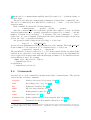

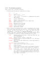


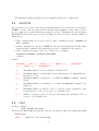

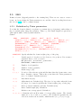
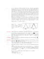
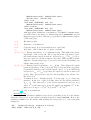
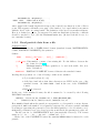
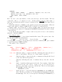
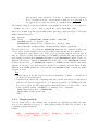
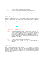
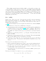


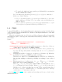
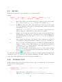
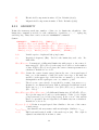


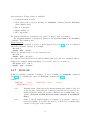


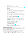
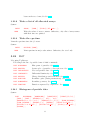

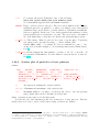
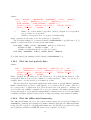
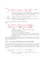


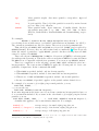


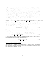
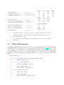
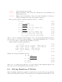
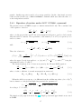
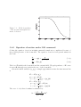

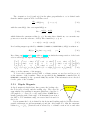

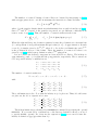

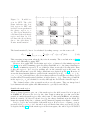
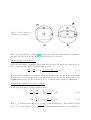


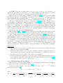
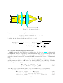
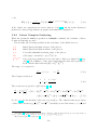
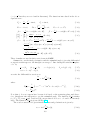
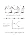

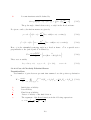


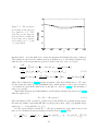

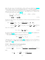
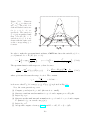

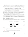
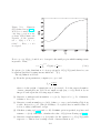


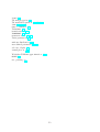


![[SU1.02.01] Notice d`utilisation du module Europlexus](http://vs1.manualzilla.com/store/data/006361860_1-614bf4408ab2aa41c7326b4178565873-150x150.png)