Download DOEK-Kit - Department of Physics and Physical Oceanography

Preface
I
DOEK-Kit
Projects in Diffractive Optics
User’s Manual
II
Preface
Warranty
Newport Corporation warrants that this product will be free from defects in
material and workmanship and will comply with Newport’s published
specifications at the time of sale for a period of one year from date of
shipment. If found to be defective during the warranty period, the product
will either be repaired or replaced at Newport's option.
To exercise this warranty, write or call your local Newport office or
representative, or contact Newport headquarters in Irvine, California. You
will be given prompt assistance and return instructions. Send the product,
freight prepaid, to the indicated service facility. Repairs will be made and the
instrument returned freight prepaid. Repaired products are warranted for the
remainder of the original warranty period or 90 days, whichever first occurs.
Limitation of Warranty
The above warranties do not apply to products which have been repaired or
modified without Newport’s written approval, or products subjected to
unusual physical, thermal or electrical stress, improper installation, misuse,
abuse, accident or negligence in use, storage, transportation or handling. This
warranty also does not apply to fuses, batteries, or damage from battery
leakage.
THIS WARRANTY IS IN LIEU OF ALL OTHER WARRANTIES,
EXPRESSED OR IMPLIED, INCLUDING ANY IMPLIED WARRANTY
OF MERCHANTABILITY OR FITNESS FOR A PARTICULAR USE.
NEWPORT CORPORATION SHALL NOT BE LIABLE FOR ANY
INDIRECT, SPECIAL, OR CONSEQUENTIAL DAMAGES RESULTING
FROM THE PURCHASE OR USE OF ITS PRODUCTS.
First printing 2006
© 2006 by Newport Corporation, Irvine, CA. All rights reserved. No part of
this manual may be reproduced or copied without the prior written approval
of Newport Corporation.
This manual has been provided for information only and product
specifications are subject to change without notice. Any change will be
reflected in future printings.
Newport Corporation
1791 Deere Avenue, Irvine, CA 92606 USA
Model Number: DOEK-KIT-TEXT
Preface
III
Confidentiality & Proprietary Rights
Reservation of Title:
The Newport programs and all materials furnished or produced in connection
with them ("Related Materials") contain trade secrets of Newport and are for
use only in the manner expressly permitted. Newport claims and reserves all
rights and benefits afforded under law in the Programs provided by Newport
Corporation.
Newport shall retain full ownership of Intellectual Property Rights in and to
all development, process, align or assembly technologies developed and other
derivative work that may be developed by Newport. Customer shall not
challenge, or cause any third party to challenge the rights of Newport.
Preservation of Secrecy and Confidentiality and Restrictions to Access:
Customer shall protect the Newport Programs and Related Materials as trade
secrets of Newport, and shall devote its best efforts to ensure that all its
personnel protect the Newport Programs as trade secrets of Newport
Corporation. Customer shall not at any time disclose Newport's trade secrets
to any other person, firm, organization, or employee that does not need
(consistent with Customer's right of use hereunder) to obtain access to the
Newport Programs and Related Materials. These restrictions shall not apply
to information (1) generally known to the public or obtainable from public
sources; (2) readily apparent from the keyboard operations, visual display, or
output reports of the Programs; 3) previously in the possession of Customer
or subsequently developed or acquired without reliance on the Newport
Programs; or (4) approved by Newport for release without restriction.
Service Information
This section contains information regarding factory service for the source.
The user should not attempt any maintenance or service of the system or
optional equipment beyond the procedures outlined in this manual. Any
problem that cannot be resolved should be referred to Newport Corporation.
IV
Preface
Technical Support
North America & Asia
Newport Corporation Service Dept.
1791 Deere Ave. Irvine, CA 92606
Telephone: (949) 253-1694
Telephone: (800) 222-6440 x31694
Europe
Newport/MICRO-CONTROLE S.A.
Zone Industrielle
45340 Beaune la Rolande, FRANCE
Telephone: (33) 02 38 40 51 56
Asia
Newport Opto-Electronics
Technologies
中国 上海市 爱都路 253号 第3号楼 3层
C部位, 邮编 200131
253 Aidu Road, Bld #3, Flr 3, Sec C,
Shanghai 200131, China
Telephone: +86-21-5046 2300
Fax: +86-21-5046 2323
Newport Corporation Calling Procedure
If there are any defects in material or workmanship or a failure to meet
specifications, promptly notify Newport's Returns Department by calling 1-800-2226440 or by visiting our website at www.newport.com/returns within the warranty
period to obtain a Return Material Authorization Number (RMA#). Return the
product to Newport Corporation, freight prepaid, clearly marked with the RMA# and
we will either repair or replace it at our discretion. Newport is not responsible for
damage occurring in transit and is not obligated to accept products returned without
an RMA#.
E-mail: [email protected]
When calling Newport Corporation, please provide the customer care representative
with the following information:
•
•
•
Your Contact Information
Serial number or original order number
Description of problem (i.e., hardware or software)
To help our Technical Support Representatives diagnose your problem, please note the
following conditions:
•
•
•
•
•
Is the system used for manufacturing or research and development?
What was the state of the system right before the problem?
Have you seen this problem before? If so, how often?
Can the system continue to operate with this problem? Or is the system nonoperational?
Can you identify anything that was different before this problem occurred?
Preface
V
Table of Contents
Warranty
II
Technical Support
IV
Table of Contents
V
List of Figures
IX
1
10
Safety Precautions
1.1
1.2
1.3
2
General Information
2.1
2.2
2.3
3
16
Unpacking and Handling ............................................................ 16
Inspection for Damage ............................................................... 16
Parts List ..................................................................................... 16
Electrical Requirements.............................................................. 17
User’s Manual DK-LCMH-800A
4.1
14
Introduction ................................................................................ 14
Functionality............................................................................... 14
Offering Description/Comparison .............................................. 15
Getting Started
3.1
3.2
3.3
3.4
4
Definitions and Symbols ............................................................ 10
1.1.1 General Warning or Caution........................................... 10
1.1.2 Electric Shock................................................................. 10
1.1.3 CSA Mark with “C” and “US” Indicators ...................... 10
1.1.4 European Union CE Mark .............................................. 11
Warnings and Cautions............................................................... 11
1.2.1 General Warnings ........................................................... 12
1.2.2 General Cautions ............................................................ 12
Location of Warnings ................................................................. 13
1.3.1 Laser ............................................................................... 13
18
Cautions ...................................................................................... 18
4.1.1 Avoid humidity and dust ................................................ 18
4.1.2 Keep heat away............................................................... 18
4.1.3 Keep water away ............................................................ 18
VI
Preface
4.2
4.3
4.4
4.5
4.6
4.7
4.8
5
Laser Module
5.1
6
4.1.4 Avoid touching the LCD ................................................ 18
4.1.5 Cleaning the LCD........................................................... 19
4.1.6 Electrical Connections.................................................... 19
4.1.7 Housing........................................................................... 19
Technical Data............................................................................ 20
Connectors .................................................................................. 21
Connecting the DK-LCMH-800A for Usage ............................. 22
DK-LCMH-800A Control Software........................................... 23
4.5.1 System Requirements ..................................................... 23
4.5.2 Installation ...................................................................... 24
4.5.3 Start of DK-LCMH-800A Control Program .................. 24
4.5.4 Controls: Contrast, Brightness, Geometry...................... 27
4.5.5 Controls in the Field "Gamma Correction" .................... 28
4.5.6 Controls in Field "Screen Format" ................................. 29
4.5.7 Factory Defaults ............................................................. 30
RS-232 Commands..................................................................... 31
4.6.1 Command structure ........................................................ 31
4.6.2 Request Commands (Requests) ...................................... 32
4.6.3 Configuration Commands (Configs) .............................. 33
4.6.4 Other Commands............................................................ 37
Error Messages ........................................................................... 38
Assembly Drawing ..................................................................... 39
Technical data............................................................................. 40
Application Software Manual
6.1
6.2
6.3
6.4
6.5
6.6
40
42
Installation .................................................................................. 42
Starting the software................................................................... 42
Opening an Image....................................................................... 42
Full-Screen window functions.................................................... 44
Calculating a diffractive optical element (DOE)........................ 47
Creating elementary optical functions........................................ 48
6.6.1 Blank Screen................................................................... 49
6.6.2 Horizontally Divided Screen .......................................... 49
6.6.3 Random Bitmap.............................................................. 49
6.6.4 Random Binary Bitmap .................................................. 49
6.6.5 Rectangular Aperture...................................................... 49
6.6.6 Circular Aperture............................................................ 50
Preface
6.7
7
6.6.7 Binary Fresnel Zone Lens .............................................. 50
6.6.8 Fresnel Zone Lens .......................................................... 50
6.6.9 Binary Axicon ................................................................ 50
6.6.10 Axicon ............................................................................ 50
6.6.11 Concentric ring segments ............................................... 51
6.6.12 Single Slit and Double Slit ............................................. 51
6.6.13 Linear Gratings and Crossed Linear gratings ................. 51
6.6.14 Linear and Array Beamsplitter Gratings ........................ 51
6.6.15 Sinusoidal Grating .......................................................... 52
6.6.16 Blazed Grating................................................................ 52
The ‘Window’ Menu .................................................................. 52
Tutorial – Theoretical Part
7.1
7.2
7.3
8
VII
Preliminary remarks ................................................................... 53
Introduction to liquid crystal physics ......................................... 54
7.2.1 Twisted nematic LC cell................................................. 55
7.2.2 Polarization of light ........................................................ 57
7.2.3 Propagation in anisotroptic media .................................. 58
7.2.4 Waveplates ..................................................................... 59
7.2.5 Amplitude and phase modulation by a TN LC cell ........ 60
Introduction to scalar diffraction theory..................................... 62
7.3.1 Diffractive optical element (DOE) ................................. 62
7.3.2 Computer generated hologram (CGH) ........................... 63
7.3.3 Kirchhoff diffraction integral ......................................... 64
7.3.4 Fresnel approximation .................................................... 64
7.3.5 Fraunhofer approximation .............................................. 66
7.3.6 Diffraction at spatially periodic objects.......................... 67
7.3.7 Fourier transformation with a lens.................................. 68
7.3.8 Spatial frequency filtering .............................................. 69
Tutorial - Experimental Part
8.1
8.2
53
70
Projection and display characterisation ...................................... 70
8.1.1 Objective......................................................................... 70
8.1.2 Required elements .......................................................... 70
8.1.3 Set-up.............................................................................. 71
8.1.4 Suggested tasks:.............................................................. 71
8.1.5 Keywords for preparation............................................... 73
Generation and analysis of dynamic diffractive structures ........ 73
8.2.1 Objective......................................................................... 73
VIII
Preface
8.3
8.4
8.5
9
8.2.2 Required elements .......................................................... 73
8.2.3 Set-up.............................................................................. 74
8.2.4 Suggested tasks............................................................... 74
8.2.5 Keywords for preparation............................................... 76
8.2.6 Addition.......................................................................... 76
Diffractive optical elements (DOE)............................................ 76
8.3.1 Objective......................................................................... 76
8.3.2 Required elements .......................................................... 76
8.3.3 Set-up.............................................................................. 76
8.3.4 Suggested tasks............................................................... 77
Spatial frequency filtering .......................................................... 79
8.4.1 Objective......................................................................... 79
8.4.2 Required elements .......................................................... 80
8.4.3 Set-up.............................................................................. 80
8.4.4 Suggested tasks............................................................... 80
8.4.5 Keywords for preparation............................................... 81
Mach – Zehnder – Interferometer with controllable phase shift 81
8.5.1 Objective......................................................................... 81
8.5.2 Required elements .......................................................... 81
8.5.3 Set-up.............................................................................. 81
8.5.4 Suggested tasks............................................................... 82
8.5.5 Keywords for preparation............................................... 82
Maintenance and Service
9.1
9.2
83
Obtaining Service ....................................................................... 83
Service Form .............................................................................. 84
Preface
IX
List of Figures
Figure 1
Figure 2
Figure 3
Figure 4
Figure 5
Figure 6
Figure 7
Figure 8
Figure 9
Figure 10
Figure 11
Figure 12
Figure 13
Figure 14
Figure 15
Figure 16
Figure 17
Figure 18
Figure 19
Figure 20
Figure 21
Figure 22
Figure 23
Figure 24
Figure 25
Figure 26
Figure 27
General Warning or Caution Symbol ........................................ 10
Electrical Shock Symbol .............................................................. 10
CSA mark with “C” and “US” Indicators................................. 10
CE Mark ....................................................................................... 11
Locations of warnings on the Laser............................................ 13
Connectors of the DK-LCMH-800A........................................... 21
Connecting the DK-LCMH-800A for usage. ............................. 23
Starting the LC2002 control program........................................ 24
User dialog of the control program after start-up. ................... 25
Error message if no DK-LCMH-800A device has been
recognised...................................................................................... 25
Selection of COM port. ................................................................ 26
‘Gamma Correction’ controls..................................................... 28
Image orientation and image format.......................................... 29
Upload Factory Default ............................................................... 30
Factory Defaults Setting .............................................................. 31
DK-LCMH-800A assembly drawing. ......................................... 39
Geometrical size of the provided laser module.......................... 40
Image window of the application software ................................ 42
Toolbar of the full-screen window .............................................. 44
Menu entries for optical functions.............................................. 48
Polarization-guided light transmission ...................................... 55
LC cells with different applied voltages ..................................... 56
Set-up for Projection and display characterisation .................. 71
Set-up for investigation of dynamic diffractive structures....... 74
Set-up for “Diffractive optical elements” experiment .............. 77
Set-up for Spatial frequency filtering......................................... 80
Set-up for Mach – Zehnder – Interferometer experiment ....... 82
10
Safety Precautions
1
Safety Precautions
1.1
Definitions and Symbols
The following terms and symbols are used in this documentation where
safety-related issues occur.
1.1.1
General Warning or Caution
Figure 1
General Warning or Caution Symbol
The Exclamation Symbol in the figure above appears in Warning and Caution
tables throughout this document. This symbol designates an area where
personal injury or damage to the equipment is possible.
1.1.2
Electric Shock
Figure 2
Electrical Shock Symbol
The Electrical Shock Symbol in the figure above appears throughout this
manual. This symbol indicates a hazard arising from dangerous voltage.
Any mishandling could result in irreparable damage to the equipment, and
personal injury or death.
1.1.3
CSA Mark with “C” and “US” Indicators
Figure 3
CSA mark with “C” and “US” Indicators
Safety Precautions
11
The presence of the CSA mark with “C” and “US” indicates that it has been
designed, tested and certified as complying with all applicable U.S. and
Canadian safety standards.
1.1.4
European Union CE Mark
Figure 4
CE Mark
The presence of the CE Mark on Newport Corporation equipment means that
it has been designed, tested and certified as complying with all applicable
European Union (CE) regulations and recommendations.
1.2
Warnings and Cautions
The following are definitions of the Warnings, Cautions and Notes that are
used throughout this manual to call your attention to important information
regarding your safety, the safety and preservation of your equipment or an
important tip.
WARNING
Situation has the potential to cause bodily harm or death.
CAUTION
Situation has the potential to cause damage to property or
equipment.
NOTE
Additional information the user or operator should consider.
12
Safety Precautions
1.2.1
General Warnings
Observe these general warnings when operating or servicing this equipment:
• Heed all warnings on the unit and in the operating instructions.
• Do not use this equipment in or near water.
• Route power cords and other cables so they are not likely to be damaged.
• Disconnect power before cleaning the equipment. Please refer to chapter
4.1.5.
• To avoid explosion, do not operate this equipment in an explosive
atmosphere.
• Qualified service personnel should perform safety checks after any
service.
1.2.2
General Cautions
Observe these cautions when operating or servicing this equipment:
• If this equipment is used in a manner not specified in this manual, the
•
•
•
•
•
protection provided by this equipment may be impaired.
Follow precautions for static sensitive devices when handling this
equipment.
This product should only be powered as described in the manual.
There are no user-serviceable parts inside the Product.
To prevent damage to the equipment, read the instructions in the
equipment manual for proper input voltage.
Adhere to good laser safety practices when using this equipment.
Safety Precautions
13
1.3
Location of Warnings
1.3.1
Laser
Figure 5
Locations of warnings on the Laser
14
General Information
2
General Information
2.1
Introduction
Main component of the “Projects in Diffractive Optics” Educational Kit is the
spatial light modulator (SLM) DK-LCMH-800A. The device is a general
purpose and easy-to-use device for displaying images by use of a
monochrome, transparent liquid crystal display (LCD). It simplifies the
application of LCD’s in experimental set-ups, e.g., for prototype development
or in research labs. The small size of the device and its comfortable control
interface are major characteristics for enabling an easy usage.
Key Features
The SLM can be used e.g. for purposes in technical optics, image projection,
machine vision, diffractive optics, pattern recognition, optical information
processing, sensing, etc.
The device is designed to be plugged to the graphics board of a personal
computer with a resolution up to SVGA format, i.e. 800 x 600 pixels. The
device converts colour signals into corresponding grey-level signals.
2.2
Functionality
The SLM can be plugged to a personal computer using the serial RS-232
port. After installing the SLM driver software the image parameters of the
LCD can be easily controlled by the computer. The driver software always
saves the current setting of the image parameters. Hence, whenever the
system is started, this latest setting will be automatically loaded.
General Information
2.3
15
Offering Description/Comparison
Five experiments with several possible questions show the wide area of
physical phenomena, which can be investigated experimentally with the
“Projects in Diffractive Optics” Educational Kit. These are e.g. optical set-up
of a projector, properties of polarized light, optical properties of liquid
crystals, phase- and amplitude modulation of light fields, diffraction of light
at dynamically changing structures, diffractive optical elements (DOE’s) and
the combination, Spatial frequency filtering and interferometry (phase
shifter).
Thus the device is suitable for introductory and advanced laboratory classes
in physics and engineering study courses.
16
User´s Manual DK-LCMH-800A
3
Getting Started
3.1
Unpacking and Handling
- do not touch the LCD
3.2
Inspection for Damage
WARNING
Do not attempt to operate this equipment if there is evidence of
shipping damage or you suspect the unit is damaged. Damaged
equipment may present additional hazards to you. Contact
Newport technical support for advice before attempting to plug
in and operate damaged equipment.
3.3
Parts List
•
•
•
•
•
(1) DK-LCMH-800A: LCD image display device (SLM)
(1) PS-LCMH-1: Power supply 15V= / 0,8A
(1) 232-CBL-M/M : RS-232 adapter cable
(1) VGA-CBL-LCMH : VGA monitor cable
(1) DOEK-HLD: Mounting ring for laser module
•
•
(1) LD-635-20MM: Beam expander laser module / focus adjustable
(1) PS-LD-DOEK: Power supply 5V / 1A
•
•
(1) DK-LCMH-800A User’s Manual
(1) DOEK-KIT-CD: CD-ROM with
Driver-Software
Application Software
DOE sample structures
User´s Manual DK-LCMH-800A
•
•
•
•
•
•
•
17
(1) MRL-12M: 12” Micro Optical Rail
(5) MCF: Flat Carrier
(4) VPH-2: 2” Post Holder
(4) SP-2: 2” Post
(2) LH1-1R: 1” Lens Holder
(2) LM1-R: Lens Mount
(1) 12454: Polarizer Disk
If you are missing any hardware or have questions about the hardware
you have received, please contact Newport Corporation.
3.4
Electrical Requirements
Before attempting to power up the unit for the first time, the following
precautions must be followed:
WARNING
To avoid electric shock, connect the instrument to properly
earth-grounded, 3-prong receptacles only. Failure to observe
this precaution can result in severe injury.
18
User´s Manual DK-LCMH-800A
4
User’s Manual DK-LCMH-800A
4.1
Cautions
The DK-LCMH-800A (SLM) is an electro-optical device of high quality and
value. In order to operate and maintain the SLM in a proper manner, be sure
to read this manual carefully.
4.1.1
Avoid humidity and dust
Do not use the SLM outside buildings and in humid or dusty places.
4.1.2
Keep heat away
Keep the SLM away from extreme heat as it may cause damage. When using
the SLM its display case and power pack become warm. Take care for
sufficient ventilation, and keep the devices away from heat such as heating
radiators, strong sun light, etc.
If you plan to apply the SLM with powerful light sources, heat-protection
filters must be introduced between light source and LCD matrix. We strongly
recommend you to consult Newport in this case.
4.1.3
Keep water away
If water or some other liquid is spilled into the SLM device serious damage
can occur. Please, consult Newport services in such a case.
4.1.4
Avoid touching the LCD
User´s Manual DK-LCMH-800A
19
Avoid touching the LCD because this might cause damage to it or reduce its
optical quality.
4.1.5
Cleaning the LCD
Wipe the LCD very carefully with a soft, dry and clean cloth or with
compressed air. If you are not sure if and how to clean the LCD, consult
Newport services.
4.1.6
Electrical Connections
Connect the SLM only to other components if the power supplies of all
components are switched off. For power supply of the SLM use only the
power pack plug which is delivered with the SLM.
4.1.7
Housing
Do not open and touch the SLM device as this is dangerous and may
seriously damage it. Do not attempt to disassemble the SLM. There are no
user serviceable or adjustable parts inside.
NOTE
If the stated cautions are disregarded, the warranty claim expires.
20
User´s Manual DK-LCMH-800A
4.2
Technical Data
Display:
Type:
SONY LCX016AL
Colours:
Grey-level image playback
Active Area:
26,6 mm x 20,0 mm (1,3")
Number of image pixels:
832 x 624
Pixel Pitch:
32 µm
Image frame rate:
max. 60 Hz
Contrast ratio:
typically 200:1
Device:
Dimensions (L x W x D):
82 mm x 82 mm x 23 mm
Weight:
0,15 kg
Operating voltage of power pack plug: 100-240 V DC, 50-60 Hz
Power input of power pack plug:
max. 150 mA
Operating voltage of LC2002:
15 V AC + 5%
Positive terminal at inner pin
Power input of LC2002:
ca. 250 mA
User´s Manual DK-LCMH-800A
4.3
21
Connectors
1
8
5
1
9
1
2
Figure 6
6
3
Connectors of the DK-LCMH-800A.
The device provides three female connectors. As depicted in Figure 6, these connectors
are:
1. the serial port connector for configuration of the device
2. the power supply connector
3. the VGA video input connector
4.3.1.1
Serial Port
Configuration of serial port connector (1):
Pin 1
+5V AC Pin 5 RXD
Pin 2
+5V AC Pin 6 CTS
Pin 3
TXD
Pin 7 GND
Pin 4
RTR
Pin 8 GND
Connection parameters:
Transfer rate 4800 - 19200 Bit/s
Data bits
8
Parity
No
Stop bits 1
Data flow control Hardware handshake RTR / CTS
22
User´s Manual DK-LCMH-800A
4.3.1.2
Power Supply
The direct current (DC) connector (2) is used for power supply of the device.
The power pack cable (15 V) has to be plugged to this connector. The
positive terminal is the inner connector pin.
4.3.1.3
Video Input
The video input (3) must be connected to the graphics board of a personal
computer using the VGA adapter cable delivered with the SLM. The
computer is used as the source of image and video data. The connector
configuration is specified as follows:
4.4
Pin
Function
1
Red colour signal
2
Green colour signal
3
Blue colour signal
4
HSYNC (line synchronisation signal)
5
VSYNC (image synchronisation signal)
6
GND red colour signal
7
GND green colour signal
8
GND blue colour signal
9
GND
Connecting the DK-LCMH-800A for Usage
For using the SLM at least one computer with an VGA graphics board is
required. The computer is required for controlling the SLM and providing
images or videos to be displayed on the LCD. Instead of the PC, a VGA
camera can be used as image-signal source.
First, the SLM driver software must be correctly installed on the computer.
Then, the computer can be connected to the SLM as shown in Figure 7.
User´s Manual DK-LCMH-800A
23
Attention: Plug the serial port and VGA connector first and the power supply
connector always at last.
Figure 7
Connecting the DK-LCMH-800A for usage.
4.5
DK-LCMH-800A Control Software
4.5.1
System Requirements
•
IBM- or compatible PC
•
Processor: 80486 or Pentium
•
32 MB main memory or more
•
VGA graphics board
24
User´s Manual DK-LCMH-800A
4.5.2
•
Free RS-232 port (COM1 or COM2)
•
CD-ROM drive
•
Operating systems: Windows 95, 98, 2000 and XP
Installation
For installing the control software execute the program SETUP.EXE on CDROM. This program requests for all information required for the installation
process.
After the installation has been completed successfully, the SLM control
software can be started from the Microsoft Windows ‘Start menu’ as shown in
the next section.
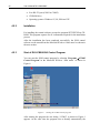
4.5.3
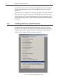
Start of DK-LCMH-800A Control Program
You can start the SLM control program by selecting ‘Programs→LC2002
Control Program’ in the Microsoft Windows ‘Start menu’ as shown in
Figure 8.
Figure 8
Starting the LC2002 control program.
After starting the program the user dialog ‘LC2002’ as shown in Figure 9
appears. At the same time the program tries to identify automatically the
User´s Manual DK-LCMH-800A
25
SLM display that should be connected to the RS-232 port (COM1 or COM2).
If the identification succeeds, the coloured ‘Connected’ sign appears in the
lower right corner of the dialog window.
In the title of the dialog window the version of the LC2002´s firmware and its
individual series number are displayed.
Figure 9
User dialog of the control program after start-up.
If no SLM device is found to be connected to the RS-232 interface, the error
message in Figure 10 will be displayed.
Figure 10
Error message if no DK-LCMH-800A device has been recognised
26
User´s Manual DK-LCMH-800A
In this case, confirm the message to make the program change into the
demonstration mode. In this mode no commands are directed to RS-232 port.
Then, check if all cables are properly connected to their corresponding ports.
It is also possible to select the COM port from the user dialog. This is shown
in Figure 11 where the COM2 port is selected from the menu ‘Options’→
’Select Port’→’COM2’. The currently used COM port is marked by a tick.
Figure 11
Selection of COM port.
If the selected port is still free, then the status message
‘COM 2 opened’
is displayed in the status bar in the bottom left of the dialog. In case the
selected COM port does not exist or is not free, the message in the status bar
states
‘COM 2 already in use or not available’ .
Now, if the selected COM port is free, select from the menu
‘Options→Check Connection’ to establish the connection to the SLM. If
the SLM is correctly connected as described in section 4.4, it is automatically
identified and its configuration data are transmitted to the control program.
The user dialog displays the mostly used parameter controls in the field
‘Contrast / Brightness / Geometry’.
User´s Manual DK-LCMH-800A
4.5.4
27
Controls: Contrast, Brightness, Geometry
The field ‘Contrast / Brightness / Geometry’ is obtained by selection of
‘Adjustments→Video’ from the menu and pushing the F2 button.
The controls are
Contrast Control
This control can be used to modify the image contrast.
Brightness Control
This control can be used to modify the image brightness.
Image Width Control
This control can be used to modify the image width. Many technical
applications require a very exact control of the image width. For this purpose
a test image with a fine stripe pattern is used. If the image width is not
adjusted exactly, a Moiré pattern results from the stripe pattern and the pixel
structure of the LCD matrix. This Moiré pattern can be seen in the projected
test image and vanishes when the image width is correctly adjusted.
Horizontal Image Position Control
This control can be used to modify the horizontal image position.
Vertical Image Position Control
This control can be used to modify the vertical image position.
Image Sharpness Control
This control can be used to modify the image sharpness. Many technical
applications require a very exact control of the image width. For this purpose
a test image with a fine vertical stripe pattern and a bright-dark transition is
recommended to be used. If the image sharpness is not exactly adjusted,
shadow effects (‘ghosts’) can appear. However, if the adjustment is corrected
the stripe pattern is rich in contrast and sharpness, and no ghost patterns
appear.
28
User´s Manual DK-LCMH-800A
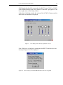
4.5.5
Controls in the Field "Gamma Correction"
The ‘Gamma Correction’ function of the SLM is supposed to be used in
advanced experiments, as it requires experiences to be used in an effective
manner. The ‘Gamma Correction’ controls, shown in Figure 12, can be
accessed by the menu option ‘Adjustments→Gamma Control’ or by
pushing the F3 key. These controls influence the linearity of the transmission
of image brightness signals. Within certain limits, the ‘Gamma Correction’
can be used to equalise non-linearities in the LCD´s transformation of
electrical signals into optical transparency signals.
Figure 12
‘Gamma Correction’ controls.
There are four different controls the resulting effect of which is depicted by
the image of the transfer function in the centre. Depending on which control
is selected the image of the transfer function changes respectively. The greyscale is used to visualise which video signals, corresponding to grey levels
and image location, are influenced by a control.
Black-Level Control
This control operates on the gamma correction of ‘darker’ image pixels. The
control shifts the given correction entry-point onto a certain grey level. With
respect to this point all ‘darker’ image pixels, and corresponding image
locations, are gamma-corrected.
User´s Manual DK-LCMH-800A
29
Black-Level Gain
This control specifies the intense of the correction effect on dark image
pixels, i.e. the increase of the intense beyond the correction entry-point.
White-Level Control
This control operates on the gamma correction of ‘brighter’ image pixels. The
control shifts the given correction entry-point onto a certain grey level. With
respect to this point all ‘brighter’ image pixels, and corresponding image
locations, are gamma-corrected.
White-Level Gain
This control specifies the intense of the correction effect on bright image
pixels, i.e. the increase of the intense beyond the correction entry-point.
After first start-up of the control program all ‘gamma correction’ controls are
set to zero, i.e., they have not effect. In order to use the gamma correction in
a sensible manner suitable test images and optical instruments for measuring
the LCD´s transmission properties are required.
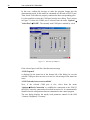
4.5.6
Controls in Field "Screen Format"
The screen format controls, shown in Figure 13, can be used to modify the
image resolution an orientation. They can accessed by the menu option
‘Adjustments → Screen Format’.
Figure 13
Image orientation and image format.
30
User´s Manual DK-LCMH-800A
You can use the buttons on the left hand side to mirror the image on the LCD
in both directions. This is helpful to make optical experiments more
comfortable.
Right Button
Pushing this button mirrors the image horizontally.
Up Button
Pushing this button mirrors the image vertically.
Format Button
Pushing this button you can select the image format to be applied.
Three standard image formats, SVGA, VGA and PC-98 are offered for
selection. The image is always displayed in a pixel-synchronised manner.
That means, images of formats with less than 800 x 600 pixels are centric
positioned and have a surrounding black frame.
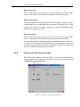
4.5.7
Factory Defaults
At every time the driver’s configuration memory can be reset to the delivery
state. To do this, select ‘Upload Factory Defaults’ from the ‘Adjustments’
menu, shown in Figure 14.
Figure 14
Upload Factory Default
User´s Manual DK-LCMH-800A
31
As shown in Figure 15 a new user dialog appears. Just load the pre-selected
factory.ini. This will reload the Factory Defaults.
The lc2002.ini is used for manufacturer’s settings only and should not utilised
by customers.
Figure 15
Factory Defaults Setting
Remarks: All adjustments effect the display immediately but need at
least 10 seconds to be permanent.
4.6
RS-232 Commands
4.6.1
Command structure
The SLM control program uses RS-232 commands to perform its tasks on the
LCD. In principle, these commands can be also send by another control
device. This makes it possible to integrate the SLM in prototype systems
where the control unit may be a different device than a PC. In the following
we describe the RS-232 commands that are used to control the SLM.
The RS-232 commands are strings of ASCII symbols that have to end with an
end symbol. An end symbol is used to separate a command from its
subsequent one and trigger the LC2002 to decode and execute the command.
Specified end symbols are Carriage Return (0Dh), Line Feed (0Ah) and
semicolon (3Bh).
32
User´s Manual DK-LCMH-800A
For the commands there is no distinction between capital and small letters.
Generally, blanks are not allowed in a command unless they are directly in
front of an end symbol.
The SLM device has an „echo“ function that confirms each correctly decoded
command. After successful decoding the string „OK“is sent by the SLM to
its RS-232 interface. In case of a false command or an unsuccessful execution
the SLM send an error code, e.g., „ERR 3“. The list and meaning of all error
codes is given in section 4.7.
The echo function can be switched on and off. When the device is switched
on, the echo function is automatically switched on as well.
In the following all available commands and their meaning are described. The
commands are ended with <CR>, respectively. The response of the SLM to
each command is written indent.
Remark: The symbol <CR> is obtained by pressing the enter button (↵) on
the keyboard. So, do not use the symbols „C“ and „R“.
4.6.2
Request Commands (Requests)
Request commands always result in a response of the SLM. They are
characterised by a question mark at the end of the command, followed by an
end symbol.
4.6.2.1
Request the device ID number
IDN?<CR>
LC2002A
4.6.2.2
Request the firmware version
VER?<CR>
1.07
User´s Manual DK-LCMH-800A
4.6.2.3
33
Request the configuration
CONF?<CR>
4 1E BE 13
0
0
0
1
0
0
5 1C
CC 77 FF A7
0
0
A
0
0 89
D 15
F
A 3C
6
The response values shown here are examples and can vary with respect to
the configuration of the device. The meaning of the bytes can be obtained
from the following table. The bytes specify user-specific as well as deviceinternal configurations.
4.6.3
Configuration Commands (Configs)
Configuration commands consist of a command name and a parameter value
that is separated from the name by a colon. The parameter value must be
given as an integer.
Byte No.
Meaning
0
1
2
3
4
5
Most significant byte PLL factor
Least significant byte PLL factor
HPOS, image position horizontal
VPOS, image position vertical
Internal configuration
SHP, pixel synchronicity of image playback
6
7
8
9
10
11
12
13
14
15
16
Internal configuration
Internal configuration
Internal configuration
Internal configuration
Internal configuration
Internal configuration
MODE, image format switching
DIR, e.g. scanning direction
GCW, entry point gamma corrector white
GCB, entry point gamma corrector black
GGW, enhancement gamma corrector white
17
GGB, enhancement gamma corrector black
Internal
symbol
HDN
HCKP
HSTP
CLPP
SHD
SH
MBK
34
User´s Manual DK-LCMH-800A
18
19
20
21
22
23
24
25
26
27
4.6.3.1
BRT, brightness (medium transparency
CON, contrast
Internal configuration
Internal configuration
Internal configuration
Internal configuration
Internal configuration
Internal configuration
ID number, Most significant byte
ID number, Least significant byte
BLIM
WLIM
SBRT
SID
VCOM
CENT
Image width
Parameter
Command name
PLLP
min.
848
max.
2045
Example:
PLLP:1054<CR>
OK
The parameter influences the pixel synchronicity of the image playback. For
the image format SVGA (800 x 600 image pixels) usually 1054 is the correct
value.
4.6.3.2
Horizontal image position
Parameter
Command name
HPOS
Example:
HPOS:207<CR>
OK
min.
0
max.
255
User´s Manual DK-LCMH-800A
4.6.3.3
35
Vertical image position
Parameter
Command name
VPOS
min.
max.
0
255
Example:
VPOS:19<CR>
OK
4.6.3.4
Pixel phase (pixel synchronicity)
Parameter
Command name
SHP
min.
0
max.
15
Example:
SHP:1<CR>
OK
4.6.3.5
Image format
Command name
MODE
Parameter
Meaning
SVGA 800x600 (CCh)
204
PC-98 640x400 (C9h)
201
VGA 640x480 (CEh)
206
Example:
MODE:204<CR>
OK
Remark: When setting the image format using the MODE command, the
pixel-synchronised playback is preserved. Image formats that that do not fill
up the display are automatically centred and surrounded by a black frame.
36
User´s Manual DK-LCMH-800A
4.6.3.6
Entry point of gamma correction white
Parameter
Command name
GCW
min.
max.
0
255
Example:
GCW:1<CR>
OK
4.6.3.7
Intense of gamma correction white
Parameter
Command name
GGW
min.
max.
0
255
Example:
GGW:1<CR>
OK
4.6.3.8
Entry point of gamma correction white
Parameter
Command name
GCB
min.
max.
0
255
Example:
GCB:1<CR>
OK
4.6.3.9
Intense of gamma correction black
Parameter
Command name
GGB
min.
0
max.
255
User´s Manual DK-LCMH-800A
37
Example:
GGW:254<CR>
OK
4.6.3.10
Contrast
Parameter
Command name
CON
min.
0
max.
255
Example:
CON:196<CR>
OK
4.6.3.11
Brightness
Parameter
Command name
BRT
min.
0
max.
255
Example:
BRT:183<CR>
OK
4.6.4
Other Commands
4.6.4.1
Echo switching on/off
The command ECHO:OFF<CR> suppresses the mandatory response with OK
on each correctly decoded command or error code messages. The command
ECHO:ON<CR> can be used to switch the echo on again.
38
User´s Manual DK-LCMH-800A
4.7
Error Messages
The meaning of error messages is given in the following list:
ERR 1 Overflow of the symbolreceiving buffer
ERR 2 Unexpected symbol in
command (neither letter,
digit, nor underscore)
ERR 3 Unknown command
ERR 4 Parameter of preceding
command not allowed
ERR 5 Unknown parameter
ERR 6 Unexpected symbol in
parameter (neither letter,
digit, nor underscore)
ERR 7 Digit was expected but a
different symbol received
ERR 8 Command did not end
correctly; instead of end
symbol another symbol was
received
ERR 9 Command parameter
missing
ERR
Internal error (EEPWR)
10
ERR
Internal error (EEPRD)
11
ERR
Internal error (DACWR)
12
ERR
Internal error (EPTWR)
13
ERR
Internal error (RESTORE)
14
RS-232
handshake
does not work,
internal or
external error
Command
incorrect
Command
incorrect
Parameter
incorrect
Parameter
incorrect
Parameter
incorrect
LC2002 defective
LC2002 defective
LC2002 defective
LC2002 defective
LC2002 defective
User´s Manual DK-LCMH-800A
Assembly Drawing
In order to assemble the SLM device on one side four drill-holes M2 are
provided.
Caution: The assembly screws must not go deeper than 8mm into the box.
Figure 16 presents the SLM assembly drawing. The dimension values are
given in mm.
82,0
M2
31,0
4.8
39
31,0
82,0
Figure 16
DK-LCMH-800A assembly drawing.
40
Laser Module
5
Laser Module
5.1
Technical data
Wavelength:
532 nm
Operating voltage:
5 V (DC)
Power input:
< 250 mA
Aperture:
15-20 mm
Output power:
1 mW
Beam diameter:
focus adjustable
Operating temperature: 15°C ~ 30°C
Laser class:
Class 2 laser with FDA registration
Figure 17
Geometrical size of the provided laser module.
Laser Module
41
The provided laser is a class 2 laser module.
Class 2 laser products can emit 1 mW of accessible laser
emission. A class 2 laser can cause eye damage if a
person deliberately forces himself to stare into the beam
despite the strong natural reflex to avert his gaze.
Do not look into the laser beam or on any reflections!
Some basic guidelines for Laser Safety:
1. Never look into the beam of any laser.
2. Be aware of the hazards posed by your laser.
3. Aim the laser well away from others.
4. Use an appropriate target.
5. Do not allow the beam to inadvertently reflect from metal or glass
surfaces.
6. Use protective eyewear.
Certain preventive measurements have to be done before the usage of the
provided laser. Inform yourself about applicable regulations with laser
products of the class 2 and consider these by application of the laser.
NEWPORT assumes no liability for any damage caused by the laser.
42
Application Software Manual
6
Application Software Manual
6.1
Installation
Start “installer.exe” and follow the instructions of the installation menu.
Please accept the license agreement before choosing the required program
components. Mark all checkboxes to install the complete version. Choose the
destination folder as well as the start menu folder. Click “Install” to start the
installation procedure and click finally “Close” to finish the installation.
6.2
Starting the software
Start the program using the start menu entry “Application Software” .
6.3
Opening an Image
Figure 18
Image window of the application software
Application Software Manual
43
Choose from the File menu the point „Open Image File“. Possible image
formats that can be opened are JPG, BMP, PNG, PGM. The loaded picture
will be transformed to a 256 grey scale picture. In order to display all 256
gray scales a monitor setting of minimum 16 Mio. colours (24bit) is required.
The image window will have the following buttons:
‘Zoom In’ Button
Pushing this button will perform a fast ‘zoom in’ operation on the image.
‘Zoom Out’ Button
Pushing this button will perform a fast ‘zoom out’ operation on the image.
‘Save’ Button
Pushing this button will open a dialog in which a file name can be specified
for saving the image in one of the supported formats (PNG or BMP Image,
ASCII textfile matrix of integer values representing the grayscale values).
‘Compute DOE’ Button
This button will only appear if the displayed image (taking zoom operations
into account) is no larger than 200x200 pixels.
Pushing this button will start a computation of a Computer-generated
hologram (CGH) phase function for the signal displayed in the image
window. Please see section 6.5 for more information.
The result of the computation will be displayed in a full-screen window
where it can be manipulated as explained in section 6.4.
‘Replicate to full screen size’ Button
Pushing this button will open a full-screen window in which the shown image
is used as a single tile which is replicated until the whole screen is covered.
44
Application Software Manual
6.4
Full-Screen window functions
This full-screen image will display a task-bar immediately after its
appearance. This taskbar will disappear but emerge again when the position
of the mouse pointer of the PC is moved towards the right edge of the
window.
Indicator for
currently active
toolbar button
Slider and
value indicator
for parameter
Zoom of basic
tile image
Toolbar button
explanation
appears
Figure 19
Toolbar of the full-screen window
The functions accessibly by the taskbar buttons offer the possibility to
manipulate the ‘basic tile’ image by superposition of signals that represent
optical elements (lens, prisms), by zooming and translating the image and by
changing its grayscale values.
Application Software Manual
45
The taskbar will have the following buttons:
‘Zoom In’ Button
Pushing this button will perform a fast ‘zoom in’ operation on the image that
is the basic tile of the displayed image composition. Note that the zoom does
not change superimposed optical functions, it will only be applied to the
‘basic tile’.
‘Zoom Out’ Button
Pushing this button will perform a fast ‘zoom out’ operation on the image
that is the basic tile of the displayed image composition. Note that the zoom
does not change superimposed optical functions, it will only be applied to
the ‘basic tile’.
‘Save’ Button
Pushing this button will open a dialog in which a file name can be specified
for saving the full-screen image image in one of the supported formats (PNG
or BMP Image, ASCII textfile matrix of integer values representing the
grayscale values). The image will be saved as displayed, i.e. including effects
by superposition of optical functions etc.
‘Superimpose lens’ Button
This button will superimpose the displayed image with a XY grayscale signal
that resembles the optical phase function of a lens. This means that the focal
plane of the light source incident on the LC Display is changed when such
function is superimposed.
The focussing/defocussing strength of the optical lens function can be
changed by adjusting the value given on the task bar by moving the slider or
by directly entering a value.
‘Superimpose prism in X direction’ Button
Pushing this button will superimpose the displayed image with a grayscale
signal that resembles the optical phase function of a prism in X direction.
This means that all diffraction angles created by the signal on the LC Display
are changed when such function is superimposed.
46
Application Software Manual
The strength of the optical prism function can be changed by adjusting the
value given on the task bar by moving the slider or by directly entering a
value.
In order to switch to a prism superposition in Y direction, click on the button
again.
‘Superimpose prism in Y direction’ Button
Pushing this button will superimpose the displayed image with a grayscale
signal that resembles the optical phase function of a prism in Y direction.
This means that all diffraction angles created by the signal on the LC Display
are changed when such function is superimposed.
The strength of the optical prism function can be changed by adjusting the
value given on the task bar by moving the slider or by directly entering a
value.
In order to switch back to a prism superposition in X direction, click on the
button again.
‘Adjust Graylevel 1’ Button
This button will only be accessible if the ‘basic tile’ image is binary, i.e.
consists of only two different graylevel values.
Pushing this button will than permit a change of one of the two grayscale
values by moving the slider or by directly entering a value.
‘Adjust Graylevel 2’ Button
This button will only be accessible if the ‘basic tile’ image is binary, i.e.
consists of only two different graylevel values.
Pushing this button will than permit a change of the second of the two
grayscale values by moving the slider or by directly entering a value.
‘Adjust Gamma curve’ Button
This button will be accessible if either the ‘basic tile’ image is binary and a
lens and/or prism functions are superimposed, or if the ‘basic tile’ image is
not binary.
Application Software Manual
47
Pushing this button will than permit a simultaneous change of all grayscale
values by moving the slider or by directly entering a value. The gamma curve
is linear if the entered value is 0, and can be changed to concave and convex
nonlinear curves by entering positive and negative values, respectively.
‘Invert displayed bitmap’ Button
This toggle button will invert the grayscale value of the displayed full-screen
image. This includes any superimposed lens and or prism functions. This
inversion can be reversed simply by clicking the button again, which will
cause the button to be no longer toggled.
‘Translate in X direction’ Button
Pushing this button will move the shown image with respect to the X
direction. This function can be used to align the displayed functions with
respect to the incident beam. Note that the translation does change the ‘basic
tile’ and any superimposed optical functions (if present) simultaneously.
In order to switch to a translation in Y direction, click on the button again.
‘Translate in Y direction’ Button
Pushing this button will move the shown image with respect to the X
direction. This function can be used to align the displayed functions with
respect to the incident beam. Note that the translation does change the ‘basic
tile’ and any superimposed optical functions (if present) simultaneously.
In order to switch back to a translation in X direction, click on the button
again.
6.5
Calculating a diffractive optical element (DOE)
To compute a DOE, the signal image size needs to be smaller than 200x200
pixel. DOE computation for larger pictures is not supported by this software.
Load the image as described in section 6.3. If the image is not larger than
200x200 pixel the ‘Compute DOE’ Button will appear with the option to
calculate a diffractive optical element (DOE) for this image. Press this button
48
Application Software Manual
to start the iterative Fourier Transformation Algorithm (IFTA). Note that the
process of computing may take a while, depending strongly on the signal
picture size.
When the process is finished, two windows will appear. They show the DOE
phase function (in a full-screen window) and the calculated intensity of the
diffraction pattern. This calculated intensity should look quite similar to the
image in the original window, if the DOE calculation algorithm has properly
converged.
6.6
Creating elementary optical functions
All optical functions from the menu point Elementary Optical Functions
appear in a new windows after input of the required parameters. Depending
on the optical function, binary or multilevel, the task bar of the full-screen
window will be slightly different (compare section 6.4).
Figure 20
Menu entries for optical functions
Application Software Manual
6.6.1
49
Blank Screen
(binary)
With this function you can create a homogeneous gray level screen. If the
mouse pointer is moved to the right edge of the window a taskbar for
changing the addressed gray level occurs.
6.6.2
Horizontally Divided Screen
(binary)
With this function you will create a horizontally divided screen, constitng of
two homogeneous graylevel partial screens. If the mouse pointer is moved to
the right right edge of the window a taskbar for changing the addressed gray
levels occurs.
6.6.3
Random Bitmap
(multilevel)
With this function you will create a random pixel distribution using 256
grayscale values. This function can be used to realize the optical function of a
random phase plate.
6.6.4
Random Binary Bitmap
(binary)
With this function you will create a random pixel distribution using only two
grayscale values. This function can be used to realize the optical function of a
random binary phase plate.
6.6.5
Rectangular Aperture
(binary)
Use this function to create a rectangular aperture. The size of the aperture can
be defined by specifying the aperture width and aperture height. With the
sliders on the taskbar one can change the gray levels of the background and
of the aperture.
50
Application Software Manual
6.6.6
Circular Aperture
(binary)
Use this function to create a circular aperture. The radius of the aperture can
be defined by specifying a numbers of pixels. With the sliders on the taskbar
one can change the graylevels of the background and of the aperture.
6.6.7
Binary Fresnel Zone Lens
(binary)
Use this function to create a Binary Fresnel Zone Lens graylevel image
representation. In the dialogue field the lens function can be characterized by
the radius of the smallest ring, which is defined by a number of pixels.
6.6.8
Fresnel Zone Lens
(multilevel)
Use this function to create a 256-level Fresnel Zone Lens graylevel image
representation. In the dialogue field the lens function can be characterized by
the radius of the smallest ring, which is defined by a number of pixels. It can
be specified whether the image representing the lens should be positive or
negative.
6.6.9
Binary Axicon
(binary)
Use this function to create a Binary Axicon graylevel image representation.
In the dialogue field the lens function can be characterized by the radius of
the smallest ring, which is defined by a number of pixels.
6.6.10
Axicon
(multilevel)
Use this function to create a 256-level Axicon graylevel image
representation. In the dialogue field the axicon function can be characterized
by the radius of the smallest ring, which is defined by a number of pixels. It
can be specified whether the image representing the lens should be positive or
negative.
Application Software Manual
6.6.11
51
Concentric ring segments
(binary)
Use this function to create binary images consisting of concentric ring
segments. In the dialogue field the image function can be characterized by the
radius of the smallest ring, which is defined by a number of pixels, and the
desired number of segments, which can be varied from two to 20 (even
numbers only).
6.6.12
Single Slit and Double Slit
(binary)
To create a single slit choose the point „Show Single Slit“ from the menu
point Elementary Optical Functions. The slit width can be defined by the
number of pixels in the dialog window.
To create a double slit choose the point „Show Double Slit“ from the menu
point Elementary Optical Functions. Moreover the slit distance can also be
defined. This refers to the gap between both slits.
6.6.13
Linear Gratings and Crossed Linear gratings
(binary)
Choose from the menu Elementary Optical Functions the item „Show Binary
Linear Grating“ to create a grating. The grating period can be defined by the
number of pixel. By selecting the boxes the grating direction can be chosen
horizontal and/or vertical. Check both boxes to overlap a horizontal with a
vertical grating.
6.6.14
Linear and Array Beamsplitter Gratings
(binary)
Choose from the menu Elementary Optical Functions one of the menu items
-
Show Binary Linear 1-to-5 Linear Beamsplitter Grating (Grating
period 26 Pixels)
-
Show Binary 1-to-(2x2) Separable Array Beamsplitter Grating
(Grating period 18x18 Pixels)
-
Show Binary Array 1-to-(5x5) Separable Array Beamsplitter Grating
(Grating period 26x26 Pixels)
52
Application Software Manual
-
Show Binary Array 1-to-(5x5) Non-separable Array Beamsplitter
Grating (Grating period 26x26 Pixels)
to obtain a full-screen window with one of the mentioned diffractive
elements.
The basic tiles of these gratings are fixed and usable as examples for
separable and non-separable binary DOEs.
6.6.15
Sinusoidal Grating
(multilevel)
Choose from the menu point Elementary Optical Functions „Show
Sinusoidal Grating“ to create a sinusoidal grating. The size of the grating
period can be specified by the number of pixels.
6.6.16
Blazed Grating
(multilevel)
Choose from the menu point Elementary Optical Functions „Show Blazed
Grating“ to create a blazed grating. The size of the grating period can be
specified by the number of pixels.
6.7
The ‘Window’ Menu
The Menu ‘Windows’ contains the usual options for tiling, cascading and
closing windows that are opened inside the main window.
When fullscreen windows are open outside the main window, they can be
closed via a separate menu point ‘Close all windows outside the main
window’. Of course the menu item ‘Close all windows inside the main
window’ does not affect full-screen windows outside and vice versa.
Tutorial – Theoretical Part
7
53
Tutorial – Theoretical Part
Five experiments have been chosen which demonstrate the wide range of
physical phenomena, which can be investigated experimentally with this
educational kit.
These are e.g. the optical set-up of a projector, properties of polarized light,
optical properties of liquid crystals, the modulation of phase, amplitude and
polarization of light fields, the diffraction of light at dynamically changing
structures, Diffractive Optical Elements (DOE’s), Spatial frequency filtering
and interferometry (phase shifter).
Thus the device is suitable for introductory and advanced laboratory classes
in physics and engineering study courses.
7.1
Preliminary remarks
The diffraction of light at dynamically adjustable optical elements as
represented by the LC cells of a spatial light modulator can be described by
the transmission through the LC material, which is characterized by its
electrooptical properties, and the following pattern formation due to
propagation for the diffracted wave. Diffractive optical elements (DOE’s) are
applied more and more in modern optical instruments. The optical function is
caused by the diffraction and interference of light in contrast to refractive
optical components.
The usage of diffraction and interference requires structures in the dimension
of the optical wavelength. These structures became available in the context of
modern methods of Nano-technology. Lithographical production
technologies and replication processes have made it possible that DOE’s can
be produced in mass production. Thus diffractive optical elements, which act
as lenses, prisms, or beam-splitters to create images or writings as diffraction
patterns, are easier to produce and more compact than corresponding
conventional elements, if they exist at all. A well known example are DOE’s,
which can be mounted on laser pointers to create arrows, crosses and other
patterns. Also, diffractive optical beam splitters can create beams with the
same intensity in a geometrical grid, for example to measure objectives and
54
Tutorial – Theoretical Part
telescope mirrors faster and more precisely compared to the possibility with
one beam or with mechanical scan devices.
In the tutorial a liquid crystal modulator will be used as a spatial light
modulator to create diffractive optical structures, for exploration of
dynamical diffraction structures as well as the investigation of the
functionality and the physical properties of the device itself. Liquid crystal
displays (LCD’s) with pixel sizes significantly smaller than 100 µm are used
nowadays in digital clocks, digital thermometers, pocket calculators and
video- and data projectors. Due to the low cost, robustness, compactness and
the advantage of electrical addressing with low power consumption LCD’s
are superior to other technologies. They feature an even wider spectrum of
applications than the mentioned and open further fascinating possibilities in
the frame of photonics, as a key technology of the 21st century.
Main component of the kit is a spatial light modulator based on a translucent
LCD. Five experiments (see section 8) with questions show the diversity of
topics, that can be experimentally investigated. Hence the experiments are
qualified for introductory courses and advanced laboratory in scientific
classes depending on the chosen questions.
7.2
Introduction to liquid crystal physics
Liquid crystals (LCs) are a phase of matter where the molecule order is
between the crystalline solid state and the liquid state. The LCs differ from
ordinary liquids due to long range orders of their basic particles (i.e.
molecules) which are typical for crystals. As a result they usually show
anisotropy of certain properties, including dielectric and optical anisotropies.
At the same time they show typical flow behavior of liquids and do not have
stable positioning of single molecules.
There are different types of liquid crystals, among which are nematic and
smectic liquid crystals. Nematic liquid crystals show a characteristic linear
alignment of the molecules, they have an orientational order but a random
distribution of the molecule centers. Smectic liquid crystals additionally form
layers, and these layers have a different linear orientation directions.
Therefore smectic liquid crystals have an orientational and a translational
order.
For usage in LCD’s, liquid crystals are arranged in spatially separated cells
with carefully chosen dimensions. The optical properties of such cell can be
manipulated by application of an external electric field which changes the
orientation of the molecules in a reversible way. Due to the long range order
of the molecules and the overall regular orientation, a single LCD element
features voltage-dependent birefringent properties.
Tutorial – Theoretical Part
55
The LC cells have boundaries which are needed to firstly separate the cell
and secondly to accommodate the wires needed for adressing each cell with
an independent voltage value. Because the cells are arranged in a regular twodimensional array, the cell boundaries act as a two-dimensional grating and
produce a corresponding diffraction effect.
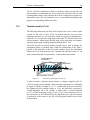
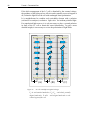
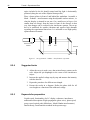
7.2.1
Twisted nematic LC cell
The following discussion will focus on LCD based on twisted nematic liquid
crystals. In the cells of such LCDs, the bottom and the top cover have
alignment structures for the molecules which are typically perpendicular to
each other. As a result of the long range order of the LC, the molecules form
a helix structure, which means that the angle of the molecular axis changes
along the optical path of light propagating through the LC cell.
The helix structure of twisted nematic crystals can be used to change the
polarization status of incident light. When the polarization of the light is
parallel to the molecules of the cell at the entrance facet, the polarization
follows the twist of the molecule axis. Therefore the light leaves the LC cell
with a polarization that is perpendicular to the incident polarization.
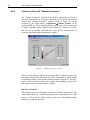
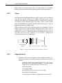
surface-aligned
molecules
light
polarization
light
propagation
twisted-nematic LC cell
Figure 21
Polarization-guided light transmission
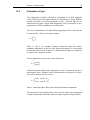
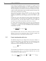
In order to realize a dynamic optical element, a voltage is applied to the LC
cell. This voltage causes changes of the molecular orientation, as is illustrated
in Figure 22 for three voltages VA, VB, VC . Additionally to the twist caused by
the alignment layers (present already at VA=0), the molecules experience a
voltage-dependent tilt if the voltage is higher than a certain threshold
(VB>Vthr). With increasing voltage (VC#Vthr), only some molecules close to
the cell surface are still influenced by the alignment layers, but the majority
of molecules in the center of the cell will get aligned parallel to the electic
field direction.
56
Tutorial – Theoretical Part
If the helix arrangement of the LC cell is disturbed by the external voltage,
the guidance of the light gets less effective and eventually ceases to happen at
all, so that the light leaves the cell with unchanged linear polarization.
It is straightforward to combine such switchable element with a polarizer
(referred to as analyzer) to obtain a ‘light valve’ for incident polarized light.
For unpolarized light sources, it is only necessary to place a second polarizer
in front of the LC cell to obtain the same functionality. To gain a more
detailed insight, it is necessary to review the polarization of light fields.
(A)
Figure 22
(B)
(C)
LC cells with different applied voltages
VA=0 with untilted molecules, VB>Vthr with tilted, partially
aligned molecules, VC#Vthr with aligned molecules in the
central region of the cell.
Tutorial – Theoretical Part
7.2.2
57
Polarization of light
The polarization of light is defined by orientation of its field amplitude
vector. While unpolarized light consists of contributions of all the different
possible directions of the field amplitude vectors, polarized light can be
characterized by either a single field component (linear polarization) or by a
superposition of field components in two directions.
The state of polarization of a light field propagating into the z direction can
be expressed by a Jones vector representation
⎛ Vx ⎞
V = ⎜⎜ ⎟⎟
⎝V y ⎠
where Vx and Vy are complex numbers which tell about the relative
amplitudes and phases of the two basic linear polarizations. It is convenient
to normalize this vector V so that |V|=1 and the field strength (i.a. amplitude)
is expressed in a separate variable.
A linear polarization is given by vectors of the form
⎛ cos α ⎞
⎟⎟
V = ⎜⎜
⎝ sin α ⎠
which tells that the polarization components in x and y direction do not have a
mutual phase delay. Arbitrary states of polarization are referred to as elliptic
polarization and are given by vectors
⎛ cos α exp(iΓ / 2) ⎞
⎟⎟
V = ⎜⎜
⎝ sin α exp(−iΓ / 2) ⎠
where Γ denotes the phase delay between the polarization components.
The expression of polarization states can be used to analyse the propagation
of light in anisotropic media like solid state matter crystals or liquid crystals.
58
Tutorial – Theoretical Part
7.2.3
Propagation in anisotroptic media
Materials which on the atomic level can be decribed as a regular arrangement
of particles in a well-defined lattice are referred to as crystals. If the material
is not isotropic, this highly ordered state of matter nevertheless leads to the
existance of optical axes in the material. Liquid crystals can be described by
the same model due to the translational order of the molecules.
Light propagation parallel to an optical axis is characterized by two indices of
refraction n1 and n2, which are usually different, and are valid for two
different states of polarization. This effect is referred to as birefringence.
Here the discussion shall be limited to uniaxial crystals, in which the
polarization states are referred to as ordinary (o) and extraordinary (eo)
polarization with refractive indices ne and no.
The impact on a transmitting light wave can be expressed by matrices which
convert the Jones vector of the incident light (see previous section) to a new
Jones vector. The different refractive indices introduce a mutual phase delay
between the two partials fields corresponding to the two linear polarizations
which are propagating with the velocities c/no and c/neo .
The transmitted light after a distance d (given by the thickness of the
material) is therefore given by
⎛ V 'o ⎞
⎛V ⎞
V ' = ⎜⎜ ' ⎟⎟ = Wd ⎜⎜ o ⎟⎟
⎝Veo ⎠
⎝V eo ⎠
where
nω
⎛
⎞
0
⎜ exp(−i o d )
⎟
c
⎟
Wd = ⎜
neo ω ⎟
⎜
0
exp(−i
d)⎟
⎜
c
⎝
⎠
An optical component with parallel entrance and exit facets made from an
uniaxial birefringent material with its optical axis perpendicular to the
direction of light propagation is referred to as a waveplate.
Tutorial – Theoretical Part
7.2.4
59
Waveplates
The matrix Wd of a waveplate can be expressed in the form
⎛
⎞
⎛ Γ⎞
⎜ exp⎜ − i ⎟
0
⎟
⎝ 2⎠
⎟
Wd = exp(iφ)⎜
⎜
⎛ Γ ⎞⎟
0
exp⎜ i ⎟ ⎟
⎜
⎝ 2 ⎠⎠
⎝
where the quantities Γ and φ are given by
Γ = (no − neo )
2π
d
λ
and
φ = 12 (no + neo )
2π
d
λ
A half-wave plate is a particular example of a waveplate with a thickness
d=
λ
2(no − neo )
so that the mutual phase delay is given by Γ=π. This means that the one
polarization direction is delayed by an optical path of half the wavelength
with respect to the other polarization. The Jones matrix of a half-wave plate is
obtained as
⎛ − i 0⎞
⎟⎟
WHWP = ⎜⎜
⎝ 0 i⎠
If the incident light is linearly polarized with an angle α of the polarization
vector to the ordinary polarization direction, its Jones vector can be expressed
by means of a rotation matrix R(α) as
⎛ Vx ⎞
⎛ V ⎞ ⎛ cos α − sin α ⎞⎛ Vo ⎞
⎟⎟⎜⎜ ⎟⎟
V = ⎜⎜ ⎟⎟ = R(α)⎜⎜ o ⎟⎟ = ⎜⎜
⎝Veo ⎠ ⎝ sin α cos α ⎠⎝Veo ⎠
⎝Vy ⎠
The matrix of a waveplate in the xy coordinate system is then given by
WWP = R(−α)Wd R(α)
60
Tutorial – Theoretical Part
For linearly polarized incident light with an angle of α=45° of the
polarization with respect to the ordinary polarization, the half-wave plate
(with the thickness d as given above) will modify the incident light as given
by the matrix
⎛ 0 − i⎞
( 45° )
⎟⎟
WHWP
= ⎜⎜
⎝−i 0 ⎠
This means that light polarized parallel to the x direction, which is assumed to
have an angle of 45° with respect to the direction of ordinary polarization,
will have its Jones vector changed from
⎛ Vx ⎞ ⎛ 1 ⎞
V = ⎜⎜ ⎟⎟ = ⎜⎜ ⎟⎟
⎝Vy ⎠ ⎝ 0 ⎠
to
⎛ 0 − i ⎞⎛ 1 ⎞ ⎛ 0 ⎞
⎛ 0⎞
⎟⎟⎜⎜ ⎟⎟ = ⎜⎜ ⎟⎟ = exp(−iπ)⎜⎜ ⎟⎟
V ' = ⎜⎜
⎝ − i 0 ⎠⎝ 0 ⎠ ⎝ − i ⎠
⎝1⎠
which corresponds to a rotation of the polarization direction by an angle
of 90°.
7.2.5
Amplitude and phase modulation by a TN LC cell
A twisted nematic LC cell can be described as a succession of a high number
of very thin waveplates which change the orientation of their optical axis
according to the change of the direction of the molecular axis. The total Jones
matrix of the cell is then obtained by matrix multiplication of all the matrices
of the assumed thin waveplates as
WTN -LC
⎞
⎛
⎛ Γ ⎞
⎛β⎞
⎟
⎜ cos χ − i⎜⎜ ⎟⎟ sin χ
⎜⎜ ⎟⎟ sin χ
2χ ⎠
χ⎠
⎟
⎜
⎝
⎝
= R(β)⎜
⎟
⎛β⎞
⎛ Γ ⎞
⎜⎜
- ⎜⎜ ⎟⎟ sin χ
cos χ + i⎜⎜ ⎟⎟ sin χ ⎟⎟
⎝χ⎠
⎝ 2χ ⎠
⎠
⎝
Tutorial – Theoretical Part
61
where is β is the total twist angle of the molecules throughout the cell and the
quantity χ is given by
χ = β 2 + (Γ / 2) 2
Even though the assumptions which are necessary for the derivation of the
Jones matrix given above require some approximations, the resulting theory
is sufficient for understanding the main optical properties of the cells.
If a LC cell satisfies β"(Γ/2), which is the case for thick cells, the Jones
matrix can be significantly simplified and permits an intuitive interpretation:
WTN -LC
⎛
⎞
⎛ Γ⎞
0
⎜ exp⎜ − i ⎟
⎟
2⎠
⎝
⎜
⎟
≈ R(β)
⎜
⎛ Γ ⎞⎟
0
exp⎜ i ⎟ ⎟
⎜
⎝ 2 ⎠⎠
⎝
If the incident light is polarized parallel to the x- or y axis the polarization
axis will be rotated by the twist angle β between the direction of the
alignment layers, as implied by the intuitive explanation illustrated in Figure
21.
If a voltage is applied to the cell, the molecules tend to align parallel to the
electric field. Thereby the anisotropy of the liquid crystal is reduced because
the angle between the direction of light propagation and the molecular axes
gets smaller until eventually both direction are parallel and the liquid crystal
appears to be isotropic (see Figure 22).
In terms of the analysis done here, the difference ∆n=no-neo gets smaller and
therefore for sufficiently high voltages one gets Γ→ 0. For this situation the
Jones matrix can be approximated as
⎛ cos β sin β ⎞ ⎛ 1 0 ⎞
⎟⎟
⎟⎟ = ⎜⎜
WTN -LC ≈ R (β) ⎜⎜
⎝ − sin β cos β ⎠ ⎝ 0 1 ⎠
which means that for a strong voltage applied to the LC cell the light
polarization is not changed.
The analysis of the intermediate cases in which the molecules are no more
aligned in the helix structure but not yet parallel to the field can be done with
the matrix WTN-LC without one of the two approximations given above. With
such analysis, the voltage-dependent optical properties can be obtained. As a
result, incident light with linear polarization leaves the cell with an elliptic
state of polarization.
62
Tutorial – Theoretical Part
However, the voltages applied to the LC cell are not directly accessible in the
SLM device contained in this kit. The voltages applied to the cells can be
controlled via a costumized electronic drive board. This drive board receives
information on what voltage should be applied to the cell as graylevel values
of the signal created by the VGA output of a graphics adapter of a common
PC.
The voltages that are applied to the cells of the LC display are in a range that
permits an almost continuous transition between the ‘helix state’ which
rotates the incident polarization to the ‘isotropic state’ in which the
polarization remains unchanged. It is obvious that by inserting an analyser
behind the display the LC display one can achieve an amplitude modulation
of a transmitting polarized light wave.
By examination of the Jones matrices WTN-LC one can also deduce that the
phase of the light passing the analyser is changed dependent on the voltagedependent parameter Γ. If the SLM is illuminated by a a coherent light
sources (e.g. a laser) various diffraction effects that are based on this phase
modulation can be observed. For the experiments it is important to note that
the incident polarization for obtaining a comparatively strong phase
modulation with only weak amplitude modulation is not parallel or
perpendicular to the alignment layers.
For the experiments dealing with diffraction effects that can be done with the
SLM, it is sufficient to understand that mutual voltage-dependent phase shifts
between the waves passing through individual LC cells can be obtained. This
means that diffractive optical elements can be realized with the help of
LCD’s. In the same way, optical elements like Fresnel lenses, gratings and
beam splitters are switchable by means of electronics.
7.3
Introduction to scalar diffraction theory
In the following some keywords will be discussed, which are important
especially for the experiments described in sections 8.2 and 8.3.
7.3.1
Diffractive optical element (DOE)
For a designated diffraction pattern a diffraction structure can be calculated
as a solution of the inverse diffraction problem and manufactured with a
suitable method. The result is a DOE, which reconstructs by illumination the
desired picture in the far field. Within certain limits lenses can be replaced by
DOE’s. DOE’s can also act as beam splitters and beam shapers or more
Tutorial – Theoretical Part
63
advanced optical elements like multi-focus lenses. A problem not yet
satisfactorily solved is the elimination of the 0th order as well as the diffused
light from other diffraction orders. However, DOE’s exhibit severe chromatic
aberrations and due to the fabrication issues, they usually will diffract light
into the 0th order, may this be desired or not. Moreover the light efficiency is
usually limited.
(Keywords: Solution of the diffraction integral, Dammann-Gitter)
7.3.2
Computer generated hologram (CGH)
Diffractive optical elements are sometimes referred to as Computer
Generated Holograms. This term was introduced because it is possible to
compute the interference pattern created by an object with a reference wave
and to fabricate an optical element from the obtained data without an
interferometric recording technique which is used for conventional
holograms.
In such recording technique, the diffuse light wave reflected by an object
interferes with a reference wave and the appearing interference wave field is
recorded in a photosensitive material or detector, in the majority of cases a
photo film. If the object wave is created by a three-dimensional object with
an irregular shape, the interference pattern leads to a structure of a complex
diffraction grating in the recording material.
A requirement for recording such a hologram is the ability for interference
(referred to as coherence) of object and reference wave field. If the hologram
is illuminated with a reference wave, it behaves like a diffraction grating and
a wave field proportional to the object wave appears in one particular
diffraction order. Thus optical waves are created that permit the threedimensional observation of the recorded object.
It is possible to compute the diffraction patterns created by object and
reference waves leading to the name Computer generated Hologram for
objects that create the same spatial wave modulation by means of a
microstructure of a swichable light modulator. For such computation, the
intensity and phase must be calculated and accordingly added for every
object and hologram point. Such computation is very demanding and
therefore CGHs which reproduce three-dimensional objects will not be the
subject of the experiments in this kit.
(keywords: off-axis, on-axis set-up, thin and thick holograms, coherence,
CGH)
64
Tutorial – Theoretical Part
7.3.3
Kirchhoff diffraction integral
A plane wave
E i = E0 ei ( kz −ωt )
propagates in z- direction and is incident onto an object at z=0. Here ω
denotes the frequency of the light and
k=
2π
λ
is the wavenumber, which is inversely proportional to the wavelength of the
light λ.
This object is assumed to be thin so that it can be described by a complex
transmission function τ(x,y). The transmitted field is
E t ( x , y , z = 0) = τ ( x , y ) E i ( x , y , z = 0)
The resulting light propagation can be described by applications of Huygens’
principle. According to this principle, a spherical wave is created by each
point (x,y) at z=0 of the diffraction structure. All spherical waves must be
added (i.e. integrated), to obtain the field amplitude from a point (x’,y’,z)
behind the diffracting object.
This description contains also waves in negative z-direction, which are not
observed. In the Fresnel-Kirchhoff diffraction theory a direction factor is
therefore introduced, which excludes the waves in negative z – direction. The
resultant field is obtained as
∞ ∞
rr
eikz
t
ik (( x ' − x ) 2 + ( y ' − y ) 2 )
E ( x' , y ' , z ) =
E
(
x
,
y
,
0
)
e
(1 + cos(ez r ))dxdy .
∫
∫
iλz −∞−∞
In general this equation is too complicated to solve diffraction problems, but
for many relevant situations suitable approximations can be used.
7.3.4
Fresnel approximation
The spatial dimension of the diffracting object should be small, compared to
the distance between object and diffraction pattern (paraxial approximation).
In this case
r r
cos(e z r ) ≈ 1
Tutorial – Theoretical Part
65
and the distance can be written as
As the amplitude is less sensitive than the phase, within the denominator the
2
2
(
(
x'− x )
y '− y )
+
r ≈ z+
2z
2z
approximation with r≈z can be used.
From this we have
E ( x' , y ' , z ) = A( x' , y ' , z ) P [ E ( x, y,0)e
t
iπ 2 2
(x +y )
λz
](ν x , ν y )
This equation describes the convolution of the transmitted field with a
impulse response of the structure. Multiplying the quadratic expression in the
exponent results in
(( x '− x )2 + ( y '− y )2 )
eikz
t
2z
E ( x' , y ' , z ) =
E
x
y
e
dxdy
(
,
,
0
)
iλz −∫∞−∫∞
∞ ∞
ik
with
eikz 2ikz (x '2 + y '2 )
A( x' , y ' , z ) =
e
iλ z
and
νx =
x'
y'
, νy =
λz
λz
which are referred to as spatial frequencies analog to the frequencies of the
Fourier transformation (above written as P) of temporal signals.
The Fresnel diffraction covers the common situation in which the observation
plane is at an finite distance behind the object.
66
Tutorial – Theoretical Part
7.3.5
Fraunhofer approximation
The Fraunhofer diffraction is a special case (and analytically a simplification)
of the Fresnel diffraction, which is valid for large distances. The Fraunhofer
approximation applies if
(x
2
+ y2
) λπ << z
is satisfied for (x,y) and (x’,y’) . In this case
E ( x' , y ' , z ) = A( x' , y ' , z ) P [ E ( x, y,0)](ν x , ν y )
with
A( x' , y ' , z ) =
exp(ikz )
iλ z
The far field in the Fraunhofer approximation is given by the Fourier
transformation of the field directly behind the diffracting object. The spatial
frequencies of the diffracting structure create waves, which propagate with
the angles
α ≈ tan α =
x'
= λν x
z
and
β ≈ tan β =
y'
= λν y
z
to the optical axis, respectively.
Thus, the far-field diffraction pattern of a spatial distribution of phase or
amplitude transmission values (given by a graylevel bitmap signal) of the
LCD can be calculated with a Fourier transformation. With the help of a lens
the far field of the light propagation can be obtained in the focal plane of the
lens (see section 7.3.7).
This means that in optics propagation of the light field realizes a Fourier
transformation in a natural way simply by propagation. The Fourier
transformation of a two-dimensional object can be observed directly in terms
of the spatial frequencies, which can be associated with diffraction orders.
These spatial frequencies can be manipulated and filtered. The Fourier
filtering is a passive parallel image processing performed at the speed of light
(see section 7.3.8).
Tutorial – Theoretical Part
67
A rather well-known application of the Fourier Transformation (FT, written
in formulas as P) is its use to compute the frequency spectrum of a timedependent signal. In Fourier optics, the signal is dependent on a spatial
coordinate rather than on a time coordinate.
Moreover, the spatial optical field is two-dimensional rather than onedimensional. In other words, in optics the corresponding variables are the
positions (x,y) and the so called spatial frequencies (νx,νy), which are linked
by the two-dimensional FT (and its inverse transformation).
F (ν x , ν y ) = P [ f ( x, y )] (ν x , ν y )
∞ ∞
=
∫ ∫ f ( x, y) exp(−2πi(ν
x
x + ν y y )) dxdy
− ∞− ∞
7.3.6
Diffraction at spatially periodic objects
Spatially periodic objects, which are often referred to as gratings, have a far
field diffraction pattern that is discrete in contrast to the contiguous
diffraction pattern produced by nonperiodic objects. The discreteness of the
spectrum of spatial frequencies contained in a periodic object leads to
maxima in the far field diffraction, which are observed at well-defined
diffraction angles and referred to as diffraction orders.
For simplicity of the discussion, only objects with a periodicity in one spatial
dimension will be treated here. If the grating period (i.e. the distance after
which the diffraction object repeats its structure) is denoted by the symbol g,
the diffraction angles ϕm can be obtained from the grating equation
g (sin(θ + ϕ m ) − sin θ) = mλ
where the incidence angle is denoted as θ, and from the simpler form
g sin ϕm = mλ
which is valid for waves incident perpendicular to the grating.
As a result, the Fourier transformation integral is simplified to a Fourier
series with coefficients Am, describing the field amplitudes of the diffracted
waves, given by
g
Am = ∫ τ( x) exp(−2πi
0
mx
) dx
g
68
Tutorial – Theoretical Part
In this formula, the diffracting object is described by a spatially resolved
complex-valued transmission function τ(x) which summarizes changes of
amplitude and phase of the transmitted wave as a function of the position.
The given integral does not take the second spatial coordinate into account,
so that it is only valid for objects with a constant transmission function with
respect to the y direction (linear gratings).
Such transmission function can be sinusoidal, as in the case of a grating
obtained by holographic recording of a two-wave-interference. The
transmission function may in this example take any value within a certain
range.
In contrast, the values of the transmission function obtained when addressing
a LCD are limited to 256 values due to the transmission of the signal as a
VGA grayscale value. The most simple example is of course a signal that
consists of only two different transmission values (binary elements).
For a binary linear phase-only grating, the structure can be described by the
transition points xk, at which the grating changes its transmission value from
τ1=exp(iΦ1) to τ2=exp(iΦ2) or vice versa. The diffraction orders obtained from
such gratings are given by
Am =
sin(∆φ / 2) N
mx
(−1) k exp(−2πi k )
∑
πm
g
k =1
for all diffraction orders with m≠0, where ∆Φ=Φ1-Φ2 denotes the phase
difference between the two transmission values. For simple examples, the
diffraction pattern can be easily analysed with this formula.
7.3.7
Fourier transformation with a lens
The diffraction image has to be changed with a lens from an infinite to a
finite-dimensional distance. The transmission of the field through the lens
results in a position depending phase shift and can be described by
multiplication with the following lens transmission function
τlens = e
−i
(
k 2 2
x +y
2f
)
The description of the diffraction occurs because of the finite distance in the
Fresnel approximation. Here ∆z is the distance behind the lens, were the
Fourier transform of the light is observed.
(x '
−i
eikz
2f
(
'
,
'
,
0
)
E
x
y
e
E ( x, y, ∆z ) =
iλ∆z −∫∞−∫∞
∞ ∞
k
2
+ y '2
)
e
(
ik
( x ' − x )2 + ( y ' − y )2
2 ∆z
)
dx' dy '
Tutorial – Theoretical Part
69
The exponents of the exponential function are quite similar. By using ∆z=f
(Shift of the observation point to the focal plane of the lens) both can be
simplified.
e ikf i 2 f (x
E ( x, y , f ) =
e
iλ f
k
=
e ikf
e
iλ f
2
)
+ y2 ∞ ∞
∫ ∫ E ( x ' , y ' ,0 ) e
ik
(( x ' x )+ ( y ' y ))
f
dx ' dy '
− ∞− ∞
(
k 2 2
i
x +y
2f
)
P [E ](
x y
, ).
λf λf
In the focus plane of a lens a field distribution is obtained, which is similar to
the Fourier transformation of the lens multiplied with a phase factor. The
corresponding intensity distribution is proportional to the intensity
distribution obtained from Fourier transformation of the incident field, which
describes its far field diffraction pattern.
7.3.8
Spatial frequency filtering
For an object placed in front of a lens having a distance d to it, the light
propagation in front of the lens can be simulated using the Fresnel
approximation of the Kirchhoff diffraction integral. The result shows that the
light in the focal plane is only changed by a phase factor dependent on d, and
for the special case d = f the field in the focus plane is equivalent to the
Fourier transformation of the field in the object plane (apart from a factor,
which does not depend on x and y).
The calculation yields
e ik 2 f i 2 f ( x
E ( x, y , f ) =
e
iλ f
k
2
+ y2
)
P [E ](
x y
, ) .
λf λf
The spatial frequency spectrum can be manipulated in the focus plane
(Transformation and inverse e.g. with 4f set-up.)
70
Tutorial – Experimental Part
8
Tutorial - Experimental Part
The first part deals with a white-light set-up, in order to demonstrate
phenomena like light polarization and basic properties of LC-Displays along
with the necessary basic geometrical optics. In the second part basic
experiments relating to diffraction and interference of light will be
performed. Part number three deals with diffractive optical elements
(DOE’s) and computer generated holograms. Basic examples of Spatial
frequency filtering in the Fourier plane are described in the fourth part.
Finally a Mach-Zehnder-Interferometer set-up is used in the fifth part. With
this interferometer the phase shift generated by the liquid crystals can be
measured. This set-up requires additional high quality optical components,
which are not included in the basic set.
8.1
Projection and display characterisation
8.1.1
Objective
Implementation of the modulator as a projection device: identification of the
mode of operation; creation of amplitude modulation by rotation of the
polarization axis of the light as a function of the applied voltage;
identification of parameters like: pixel size, length of molecule axis,
maximum phase shift; illuminating and imaging optical path.
8.1.2
Required elements
Modulator; halogen lamp with condenser (e.g. 2 bi-convex field lens f~130 to
150 mm); 2 rotary polarisers; objective lens (e.g. simple lens / iris diaphragm
and/or an achromatic lens f~80 to 130 mm) with high aperture; projection
screen; colour filter (red, blue); LDR photo resistor and Ohmmeter; optional:
iris diaphragm
Tutorial – Experimental Part
8.1.3
71
Set-up
Optical path for illumination: adjust the halogen lamp in such a way, that it
emits parallel (or slightly convergent) light. The parallel light beam should
illuminate the display completely. Make sure, that no scattered light bypasses
the display (preferably use a rectangular aperture, e.g. e made of black
cardboard, in front of the display).
Place and adjust polarisers (1st: polariser, 2nd: analyser) in front of and behind
the display in a way that the polarisation axes are 90° rotated to each other.
Address a test image onto the display.
Optical path for imaging: Place an objective lens (e.g. simple lens / iris
diaphragm and/or achromatic lens) behind the display and adjust it in such a
way, that a focused and enlarged image appears on the screen.
For measuring the parameters, the photo resistor has to be placed in the focal
plane of the lens. The total intensity will be measured this way. A neutral
density filter may be necessary to reduce the intensity. In fact a photo resistor
measures indirectly proportional but compared to a photo diode, the linear
characteristic is more than 3 orders of magnitude higher.
L1
Figure 23
8.1.4
Pol
SLM
Ana
L2
Screen/LDR
Set-up for Projection and display characterisation
Suggested tasks:
1. Measure the polarisation characteristics of the light source. (Lamp
with condenser, rotary analyser, objective lens, photo resistor)
2. Create linearly polarised light (lamp with condenser, polariser) and
measure the angle distribution of the intensity with the 2nd polariser
(analyser). Present the results in polar coordinates. Which
mathematical function describes the results? Make sure to verify the
linearity of the detector.
3. Arrange the projection set-up with illuminating and imaging beam
path. A classical photo slide is helpful and will be replaced later on by
the “polariser / LC-Display / analyser” . As objective lens try a
normal lens with different iris diaphragm apertures and the
72
Tutorial – Experimental Part
achromatic lens. Discuss the influence of the aperture regarding to the
depth of focus, brightness, influence of lens aberrations as well as the
way to avoid aberrations.
4. Set up the projection arrangement with the LC- display and optimise
the contrast. Therefore a picture has to be addressed to the monitor
and the LC – display. The picture should be imaged onto the
projection screen. Rotate the polarisers, which are perpendicular to
each other, in adequate angle steps (ca. 10°) and measure the
changing contrast quantitatively.
5. What do you observe, if one or both polarisers are removed? What do
you observe with both polarisers at best contrast, if the polarisation
position of the analyser is rotated by 45°/90°/180°? Discuss the
results. Use a grating with grating period 400 to create an image half
white half black. This image should be used to measure the contrast
with the LDR – photo resistor.
6. Determine the orientation of the molecule axis of the addressed liquid
crystal pixel from the results.
7. Determine the pixel size from the geometrical reproduction scale unit
and a e.g. rectangular image, what is defined by a specific number of
pixels on the monitor / display (use geometrical optics for
calculation). The magnification of the lens system should be known.
8. Investigate the dependency of pixel voltage and twist on the
polarization direction. Change the voltage by using different
homogeneous full screen gray level images (use the supplied
software) and measure the intensity with the LDR–photo resistor in
the focus of the objective lens. Use a projection set-up with the
optimal contrast. The results should be presented graphically. In order
to compare the results, a linear dependency should be theoretically
assumed (if necessary consider an offset). In this connection the
calculated progression of the translucent intensity as a function of the
addressed voltage should be presented in the same diagram (a detailed
calculation has to be given). Discuss the differences. Figure out a
function in which the polarisation angle on a scale from 0° to 90° can
be varied. This is possible by an appropriate choice of a polynomial
(an appropriate order/level must be chosen).
9. Repeat the experiment from point 7 using colour filters for red and
blue light.
10. For the case of maximum polarisation change the ellipticity of the
transmitted light (originally linear) should be estimated by measuring
the Stokes parameter (Set-up as used in point 7; measure the
intensities at analyser positions 0°, 45°, 90°, -45°).
Tutorial – Experimental Part
73
11. Discuss and summarize the function of an LC-display as a
polarisation modifier. Does it have influence on the amplitude or
phase of light? How can you get an amplitude modulation of light?
12. If experiment 4 “Mach-Zehnder interferometer” has already been
accomplished, please try to figure out how a separate phase and
amplitude modulation with two modulators can be realised.
8.1.5
Keywords for preparation
Polarization of light; possibility to create polarized light; optical elements for
changing the polarization state; contrast, stokes parameter; birefringence;
connection between polarisation state and angular momentum of photons;
mathematical description of a plane wave; liquid crystal; functionality of an
LC display; pixel size; fill factor; functionality of a photo resistor and
characteristic line; geometrical optic; Köhler illumination; field lens; lens
aberration; aperture
8.2
Generation and analysis of dynamic diffractive
structures
8.2.1
Objective
Implementation of the modulator to create different primary diffractive
structures, which base on phase modulation of light. Descriptive comparison
of direct changes of the diffractive pattern by changing the projected
diffractive structure. Comparison of the diffraction behaviour of complement
structures. (Babinet’s theorem). Measurement of the progression of
diffraction intensity and definition of diffraction efficiency of selected
structures. Superposition of simple diffraction pattern as a base for diffractive
optical elements.
8.2.2
Required elements
Modulator; laser with beam expander (can be used as a collimator and also to
replace the fourier lens by creating a slightly convergent beam to get a focal
plane); fourier lens (optional); one or two lenses for example (+100 or +50,
+80 or +100, -50 mm) to magnify the diffractive structure; iris diaphragm (to
eliminate the higher diffraction orders which appear due to the pixel structure
of the display); two polarisers; projection screen; digital camera or LDR-
74
Tutorial – Experimental Part
photo resistor with aperture plate 1mm or Si- photo diode on a relocatable
carriage for documentation and measurement of the diffraction structures
8.2.3
Set-up
The expanded and collimated laser beam (if no Fourier lens for focusing is
used, the laser module should be set slightly convergent to get a focus)
illuminates the display in a homogenous manner. Determine the focal plane
with the help of an adjustment paper. The image, which is created in this
plane (far field diffraction pattern), should be projected precisely. It may be
enlarged with the help of further lenses.
Higher diffraction orders can be eliminated with the iris diaphragm. Turn the
linearly polarized laser until an optimal diffraction pattern can be seen. A
digital camera can be mounted on a tripod to take pictures from the screen. A
LDR-photo resistor on a carrier can measure the diffraction pattern as well.
The whole set-up can reach a length of 2 to 2,5 m. Hence, a folded set-up
with the help of mirrors is recommended.
Polarised Laser
Module
SLM
Ana Fourier Lens
Screen/LDR
Figure 24 Set-up for investigation of dynamic diffractive structures
8.2.4
Suggested tasks
1. Preparative tasks on the computer: Create bitmap structures of a
diffraction structure in a desktop resolution of 800x600 pixel with the
software.
-
-
3 gratings with different grating period (lines + grooves) in
black and white (geometrical identical - Ronchi grating)
stripes (use the “grating functions” of the software)
an inverted grating
a 90° rotated grating
three different basic slits (choose low slit width)
three double slit arrangements
3 circular apertures and the corresponding inverse structures
Tutorial – Experimental Part
-
-
75
1 cross grating and the inverse structure
1 grating in 5 versions, in which the primary black areas are
filled with different grey levels
rectangular aperture
2. Record the projected diffraction patterns e.g. with a digital camera
and interpret them.
3. Determine the intensity distribution of the obtained diffraction pattern
and the diffraction efficiency for the gratings and the slits (I0 is the
total intensity of the central order which passes the iris diaphragm for
a non addressed modulator). The intensity distribution measurement
can be done with a LDR photo resistor or from digital camera
pictures. Compare the results with the theoretical expectations.
4. Determine the ratio of the grating period (relative to the grating with
the highest grating period) of the diffraction pattern and the bitmap
structures.
5. Determine the diffraction efficiency of the diffraction structures for
all graylevel gratings. Diffraction efficiency is defined as the ratio
between the intensities of the desired orders (e.g. the +1st and –1st
orders) and the intensities of the incident light.
6. Discuss the results of the inverted structures.
7. Discuss the diffraction structures of the circles with respect to
possible constructions of a diffractive lens (Fresnel zone lens).
8. Vary the grating period of a grating with the application software.
Explain your observations.
9. Place a horizontal grating on the left side and a vertical grating on the
right side of the monitor. Explain the observed diffraction pattern.
10. If the beam expander of the laser module is used as a collimator,
discuss the function of the Fourier lens directly behind the modulator.
If the beam expander of the laser module is used instead of the
Fourier lens, discuss why the lens function may be added to the beam
before transmitting the display.
11. Analyse the diffraction efficiency of phase- and amplitude gratings:
Place crossed polarisers in front and behind the modulator (at
maximum contrast – compare with experiment 8.1). Choose as
diffraction structure a symmetric black-white Ronchi-grating.
Measure the diffraction pattern with a camera or with the LDR-photo
resistor (aperture plate) or a Si- photo diode. Remove both polarisers,
measure once more and compare the results. Discuss the differences
in terms of the various ways of the diffraction pattern development.
12. Measure the sinc-function of the diffraction structure without iris
diaphragm and with non-addressed display.
76
Tutorial – Experimental Part
8.2.5
Keywords for preparation
Liquid crystal, functionality of a LC-display, plane wave, coherence,
diffraction, interferometry, diffraction on slit / double slit / grating / circle
aperture, mathematic description in the far field, slit function, grating
function, Fraunhofer- and Fresnel-diffraction, Babinet’s theorem, Fourier
transformation, resolution
8.2.6
Addition
If there are more laser with different wavelengths available, diffraction
pattern of different wavelengths can be analysed. The possible contrast is
depending on the wavelength.
8.3
Diffractive optical elements (DOE)
8.3.1
Objective
Creation of diffractive optical elements with the spatial light modulator,
observation of diffraction patterns in the far field, symmetry considerations
for diffraction patterns, superposition of different diffractive optical elements.
8.3.2
Required elements
Modulator; laser with beam expander (can be used as a collimator and also to
replace the Fourier lens by creating a slightly convergent beam to get a focal
plane); (Fourier-) lens f=300-400 mm (optional); two lenses (for example
+100 and –50 mm) for the enlargement of the diffractive structure in a
telescope arrangement (optional); projection screen; digital camera; optional:
one polarizer.
8.3.3
Set-up
The expanded parallel laser beam illuminates the display homogenously. A
lens with large focal length should be placed closely behind the display.
Define the focal plane of the lens with the help of an adjustment paper. The
Tutorial – Experimental Part
77
light pattern, which is observed in this plane, corresponds to the far field of
light propagation.
Higher diffraction orders can be eliminated with the iris diaphragm. A digital
camera can be mounted on a tripod to take pictures from the screen.
Polarised Laser
Module
Figure 25
8.3.4
SLM
Ana Fourier Lens
Screen/LDR
Set-up for “Diffractive optical elements” experiment
Suggested tasks
1. Address one of the provided DOE-images (preferably “grid” or
“coord”) onto the screen / display and observe the far field diffraction
pattern. Record this pattern with a camera or make a hand drawing
showing the essential features of your observations. Determine the
minimum distance for a far field observation and give an explanation
of this value. What do you observe in the near field?
Advice 1: For the analysis of the phase-DOE, no polarisers are
required. Consider the linear polarisation of the laser. The
display effects and turns the polarisation plane even in a nonaddressed state. Therefore the polarisation axis of the laser
should be adjusted by rotating the laser in order to obtain a
bright and clear diffraction pattern.
Advice 2: Display all images in full screen, because the edges of
“windows”, “buttons” and “task-bars” have an influence on the
light field which may distort the desired far field pattern.
2. Open binary images representing linear beamsplitters and array
generators. Optimize the observable diffraction pattern by adjusting
the contrast. This can be done by changing the grayscale values using
the corresponding sliders. Note down at which grayscale values the
best diffraction pattern is observed.
3. Observe the diffraction patterns in the far field
a. of the provided 5x5 binary separable array beam-splitter DOE
image
78
Tutorial – Experimental Part
b. of the provided 5x5 binary non-separable array beam-splitter
DOE image
Note down and explain your observations, especially concerning the
symmetry properties of the diffracted light pattern.
4. Observe the diffraction patterns in the far field
a. of the provided 2x2 binary array beam-splitter DOE image
b. of a checkerboard bitmap with a grating period of 18 pixels (i.e. 9
pixels line and 9 pixels groove)
c. of checkerboard bitmaps with the same grating period, but uneven
duty cycles (e.g. 12 pixels line and 6 pixels groove, 13 pixels line
and 5 pixels groove)
Why are certain diffraction orders missing for some of the DOEs ?
Hint: the images are separable, i.e. the transmission function τ(x,y) of
the LCD can be written as a product τ(x,y)=τ1(x)τ2(y). The diffraction
pattern in each direction x and y can be understood from the Fourier
series expansion of the diffraction pattern as a function to the
transition function (see section 7.3.6)
5. Change the scale of an image representing a DOE. To do this,
magnify or shrink the image using the zoom buttons of the application
software. Discuss the results.
6. Cover the image representing the DOE on the screen or just on the
display to half or ¾ size with a blacked out area. Observe each time
the light pattern in the far field. Compare them regarding the contrast
and speckles and discuss the results.
7. Place two different images representing DOEs on the screen next to
each other, so that both of them are illuminated by the laser beam
transmitting the LCD. Discuss the light pattern observed in the far
field.
8. Compute a image representing a DOE using an asymmetric image as
desired far field light pattern (use e.g. the file “newportlogo”). In a
full-screen window created from the computed DOE image, invert the
DOE using the provided toolbar button. Explain your observations.
What happens to the phase function created by the LCD when the
grayscale image is inverted ?
9. Superimpose a DOE with a lens with the application software. Create
different superpositions using different lens strengths and determine
the plane of the best observation of the diffraction pattern as a
function of the lens strength. Explain the result.
10. Create a bitmap consisting of several black and white circles. This
should be addressed with the following shapes onto the display:
Tutorial – Experimental Part
79
a. concentric full circles
b. positive and negative concentric half circles
c. positive and negative concentric quarter circles
Evaluate the diffraction patterns in the far field. Note down your
observations.
11. Use the function of the software to create a binary Fresnel zone plate.
The radius of the smallest ring can be defined to change the focal
length.
a. Try and check the “lens effect” with different radii of the
smallest ring.
b. Determine the focal length of different binary Fresnel zone
lenses experimentally as well as theoretically. Compare the
results.
c. Calculate the pixel size of the display from the focal lengths
measured for different smallest radii of the zone lenses. If
experiment 8.1 “Projection and display characterisation” has
already been accomplished, compare the obtained pixel sizes.
12. Use binary DOEs contained in the ‘elementary optical functions’ of
the application software to evaluate which symmetry the diffraction
patterns have. Calculate a DOE image for a high-contrast, asymmetric
picture of your choice with the application software.
Does the diffraction pattern you have obtained follow the symmetry
of the diffraction patterns of binary elements ? If not, why can
multilevel DOEs produce diffraction patterns with different
properties ?
13. Acquire information of how computer generated holograms of a
complex structure are created.
14. If you have done the projection experiment figure out how to get
separated phase and amplitude modulation with two SLMs.
8.4
Spatial frequency filtering
8.4.1
Objective
Projection set-up, spatial filtering in Fourier plane, high- low- pass filter,
filtering of structures
80
Tutorial – Experimental Part
8.4.2
Required elements
Modulator, laser with beam expander, (Fourier-) lens f=300-400 mm, Spatial
filter diaphragms: Iris-diaphragm, rectangle diaphragm (two razor blades),
negative hole diaphragm (middle size pinhead), projection screen, digital
camera, polarizer
8.4.3
Set-up
The expanded and collimated laser beam illuminates the display
homogenously. The linear polarisation of the laser has to be adjusted in that
way that the addressed image will be displayed with optimal contrast and
brightness. Use a (Fourier) lens with a long focal length for projection. A
focused and enlarged projection without other lenses can be created. Define
the focal plane of the lens with the help of an adjustment paper. The Fourier
image in that plane can be filtered spatially. The filtering has to be
progressed only in the central diffraction order (blind out other orders). A
digital camera can be mounted on a tripod to take pictures from the screen.
f
Polarised Laser
Module
Figure 26
8.4.4
SLM
2f
L1
Filter
f
L2
Screen
Set-up for Spatial frequency filtering
Suggested tasks
1. Why don’t you need polarisers before and behind the display? Test
the influence of an analyser behind the display.
2. Use a grating with a well known diffraction image in the Fourier
plane. Exercise the following spatial filtering:
a. block the zero diffraction order
b. keep the zero diffraction order
c. keep only higher diffraction orders (e.g. higher than 3rd order)
Tutorial – Experimental Part
81
3. Use two crossed gratings as image (chess board pattern). Carry out a
spatial filtering and see if the horizontal lines disappear on the
projection screen.
4. Design a simple image with a drawing program (black/white, lines
and filled plain). Address this image onto the display and make sure
that a clear projection is on the screen.
5. Carry out a high- and low-pass filtering in the focal plane of the
Fourier lens. Record the filtered images with a digital camera.
8.4.5
Keywords for preparation
Liquid crystal, functionality of a LC-display, phase- and amplitude
modulation, two dimensional Fourier transformation, spatial filtering, 4f
set-up, high- low- pass filtering, resolution
8.5
Mach – Zehnder – Interferometer with controllable
phase shift
8.5.1
Objective
The modulator should be used as a phase shifting element in an
interferometer set-up. Define the phase shift as a function of the
addressed voltage (important parameter of a modulator).
8.5.2
Required elements
Modulator, laser with beam expander, LDR- photo resistor or Si- photo
diode with pin diaphragm, two beam splitter (mirror or cube), two in two
axis adjustable surface mirrors
8.5.3
Set-up
The expanded (slightly collimated) laser beam illuminates a large part of
the display homogeneously. A homogenous full screen pattern is
addressed onto the display. The semiconductor laser with beam expander
82
Tutorial – Experimental Part
optics included in the kit should rotated until the light is horizontally
polarised (along the axis of the elliptical beam profile).
Place a beam splitter in front of and behind the modulator. Assemble a
Mach – Zehnder – interferometer using the adjustable surface-mirrors , in
what the display is situated in one arm. Cut a small area (as big or a bit
smaller than one fringe) from the beam in front of the detector in that
way, that changes can be realised in the interference pattern. The set-up
has to be stabilized for outside vibrations and requires high demands
regarding the experimental know-how. It is advisable to use high-quality
optomechanical elements.
BS
Polarised Laser
Module
M
SLM
Ana
Detector
M
Figure 27
8.5.4
BS
Set-up for Mach – Zehnder – Interferometer experiment
Suggested tasks
1. Adjust the set-up in such a way, that an interference pattern can be
seen. Adjust the pin diaphragm to the centre of the interference
stripes.
2. Increase the applied voltage step by step and measure the intensity
with the detector.
3. Repeat the procedure for different wavelength.
4. Present the results in a diagram. Define the phase shift for all
wavelengths as a function of the addressed voltage.
8.5.5
Keywords for preparation
Liquid crystal, functionality of a LC-display, coherence, interference,
mathematical description of light propagation (plane wave), phase-speed,
group- speed, optical path, (Michelson-, Mach-Zehnder interferometer)
interferometry, interferometric methods in the spectroscopy.
Maintenance and Service
9
83
Maintenance and Service
CAUTION
There are no user serviceable parts inside any components of
the “Projects in Diffractive Optics” Education Kit. Work
performed by persons not authorized by Newport Corporation
will void the warranty.
1.
9.1
Obtaining Service
The components of the “Projects in Diffractive Optics” Education Kit
contain no user serviceable parts. To obtain information regarding factory
service, contact Newport Corporation or your Newport representative. Please
have the following information available:
2. Instrument model number (on the device)
3. Instrument serial number ()
4. Description of the problem.
If the instrument is to be returned to Newport Corporation, you will be given
a Return Number, which you should reference in your shipping documents.
Please fill out a copy of the service form, located on the following page, and
have the information ready when contacting Newport Corporation. Return
the completed service form with the instrument.
84
Maintenance and Service
9.2
Service Form
Newport Corporation
U.S.A. Office: 800-222-6440
FAX: 949/253-1479
Name _______________________________
Return Authorization #__________________
(Please obtain RA# prior to return of item)
Company ________________________________________________________________________
(Please obtain RA # prior to return of item)
Address ________________________________ ____________________Date _________________
Country _______________________ Phone Number ______________________________________
P.O. Number ___________________ FAX Number _______________________________________
Item(s) Being Returned:
Model # _______________________ Serial # __________________________
Description _______________________________________________________________________
Reason for return of goods (please list any specific problems):
Newport Corporation
Worldwide Headquarters
1791 Deere Avenue
Irvine, CA 92606
(In U.S.): 800-222-6440
Tel: 949-863-3144
Fax: 949-253-1680
Internet: [email protected]
Visit Newport Online at: www.newport.com