1
SLAW, a package for Scaling LAWs from
statistical data
Version 0.93.
User’s Guide
Fernando Ordóñez∗, Timothy Li†, and Patricio Mendez‡
Abstract
Program SLAW derives representative scaling laws of a process
from sensitivity analysis experimental data. The approach integrates
dimensional analysis with a multivariate linear regression backward
elimination procedure. In addition to the scaling laws, the program
provides a set of dimensionless groups ranked by relevance.
The algorithm is coded as a group of Matlab .m files. This user’s
manual describes the different programs in the SLAW suite and its
Java interface, discussing its usage through an illustrative example.
1
Introduction
The objective of SLAW is to derive representative scaling laws of a process
from sensitivity analysis data from experiments of the process. The approach integrates dimensional analysis with a multivariate linear regression
backward elimination procedure. In addition to the scaling laws, the program provides a set of dimensionless groups ranked by relevance. With the
∗
Industrial and Systems Engineering, University of Southern California, GER-247, Los
Angeles, CA 90089-0193, USA, email: [email protected]
†
Industrial and Systems Engineering, University of Southern California, Los Angeles,
CA 90089-0193, USA, email: [email protected]
‡
Exponent,
21 Strathmore Road,
Natick,
MA 01760,
USA, email:
[email protected]
1
scaling laws obtained, the whole set of data can be summarized, generalized,
extrapolated, and simplified with great accuracy and physical meaning. One
advantage of this approach is that it enables engineers to simplify a problem by eliminating physical parameters, which are sometimes very difficult
to measure or obtain. Other statistical simplifications, such as the principal
directions of the matrix of correlation, reduce the mathematical complexity
of the problem but still require the use of all parameters, regardless of their
importance. For example, the thermal expansion of a solid might be very
difficult to determine, yet not relevant in a problem. Strictly mathematical
approaches might still require this parameter, while the experimental data
could indicate that thermal expansion is not relevant, and thus SLAW would
generate scaling laws in which that parameter does not appear.
This user’s manual first describes the model assumptions, the inputs and
what are the outputs of SLAW. We then describe the operation of SLAW
either through the Matlab files or through the Java interface. In the appendix
we present a list of all program files of the SLAW algorithm with their input
and output.
2
Program Objectives
The objective of SLAW is to derive the characteristic value Y (X) of some
process that only depends on n problem parameters X1 , . . . , Xn . For example
in the problem of determining the period of a pendulum, the characteristic
quantity would be the period, while problem parameters can be the length
of the pendulum, the mass, the density of the medium, etc. Note that we
are not interested in variables used to describe the evolution in a specific
realization of the process, such as position and time. We further assume that
the characteristic value is given by the following power law of the problem
parameters:
Y =a
n
Y
Pm
Xj
i=0
aij
.
(1)
j=1
SLAW identifies this power law, by separating it into the most representative scaling law and m dimensionless groups ranked by their significance
to the characteristic value:
Y =a
n
Y
j=1
a
Xj 0j
m
Y
Πi , where Πi =
i=1
n
Y
j=1
2
Xj aij ,
(2)
where a is a numerical constant. The model postulated also considers the
uncertainties, which arise from working with experimental data and considering only n independent variables and disregarding the, possibly tiny, effect of
other variables. By taking the logarithm of Equation (1), and considering the
existing uncertainties in the model, we arrive at the following multivariate
linear regression model:
n
X
log Y = β0 +
βj log Xj + ε ,
(3)
j=1
where ε is an error term and the coefficients are given by:
β0 = log a ,
βj =
m
X
aij .
i=0
Experimental data is used to estimate the coefficients in this multivariate linear regression model, by solving different linearly constrained linear
regressions, i.e. minimizing the squared sums of errors subject to linear constraints. For example the standard linear regression suggested by Equation
(3) produces a model that gives estimates of the dependent variable that do
not have the same units as Y . We explicitly impose a linear units constraint,
which constrains our search of coefficients only to those that give models
with the correct units. Additional linear constraints are also used to identify
the dimensionless groups in order of relevance to the characteristic value.
We refer the reader to [1] for a detailed description of the model and the
procedure used to identify the scaling law and dimensionless groups.
3
Inputs and Outputs
Before describing the input data for SLAW and the output obtained from
it we discuss in a bit more detail the problem of determining the period of
a pendulum. This is a well known physics example that will be used to
illustrate the use of the program.
3.1
Period of a Pendulum
For a pendulum, such as the one described in Figure 1, when the only relevant
force acting on the pendulum is the force of gravity, and for small oscillations,
3
l
water
θ
m
g
d
Figure 1: Representation of a simple pendulum and its elements
it is well known that the period of a pendulum is given by the formula:
q
T = 2π l/g
(4)
where T is the period (the dependent variable Y in this problem), l is the
length of the string, and g is the acceleration of gravity. If Expression (4) were
unknown and should be discovered from experimental data, it is reasonable
to assume that additional independent parameters Xi might be considered
to describe the period of a pendulum, such as the mass, the initial angle, and
the density of the surrounding fluid. In Table 1 we list a few parameters that
could be assumed to influence the period of a pendulum and their units:
Table 1: Parameters
symbol units
Y
T
s
X1 m
kg
X2 l
m
X3 θ
rad
X4 d
m
X5 ρ
kg/m3
X6 g
m/s2
to explain the period of a pendulum
description
period (dependent variable)
mass of the bob
length of the pendulum
initial angle
characteristic dimension of the bob
density of fluid surrounding the bob
acceleration of gravity
4
3.2
Inputs
The inputs to SLAW are two text files containing the experimental data and
the units information data, respectively.
• Experimental data: A text file with the experiment data, one experiment per row, with the value of the dependent variable Y in the first
column, and the n independent variables in the next n columns. This
file should be in a format that is readable by the Matlab function load.
Below we present the file used for the pendulum example. Note that the
experiment are conducted in order to show the effect on the period of
varying one parameter at a time. SLAW requires that the experimental
data explores how the dependent variable is affected by each parameter
through such a sensitivity analysis. We refer to such data as sensitivity
analysis data.
%
%
period
s
2.248
2.26
1.328
1.337
1.844
1.84
0.912
0.891
1.093
1.084
1.121
1.821
1.836
1.84
1.866
1.197
1.198
1.234
1.255
0.823
0.828
0.558
1.434
1.446
1.528
1.605
0.924
0.667
0.671
2.053
2.044
2.059
0.668
0.678
0.4265
0.4335
2.044
2.049
2.066
0.4795
2.818
2.868
2.884
2.918
2.944
2.896
m
kg
0.295
0.295
0.295
0.295
0.1475
0.1475
0.1475
0.1475
0.1475
0.1475
0.1475
0.05
0.05
0.05
0.05
0.05
0.05
0.05
0.05
0.05
0.05
0.05
0.02
0.02
0.02
0.02
0.02
0.02
0.02
0.005
0.005
0.005
0.005
0.005
0.005
0.005
0.001
0.001
0.001
0.001
0.05
0.05
0.05
0.02
0.02
0.02
l
m
1.265
1.265
0.435
0.435
0.84
0.84
0.192
0.192
0.287
0.287
0.287
0.816
0.816
0.816
0.816
0.354
0.354
0.354
0.354
0.158
0.158
0.085
0.502
0.502
0.502
0.502
0.202
0.11
0.11
1.025
1.025
1.025
0.106
0.106
0.042
0.042
1.037
1.037
1.037
0.052
1.6
1.6
1.6
1.6
1.6
1.6
theta
rad
0.085953704
0.171423406
0.245519496
0.466402423
0.129040859
0.255037
0.516337133
0.278987417
0.362964317
0.189342043
0.651811167
0.067300169
0.132792341
0.262203488
0.491673135
0.154134896
0.298697423
0.554015696
0.655149327
0.334982296
0.603897219
0.307567108
0.109126499
0.411364964
0.716285835
0.785398163
0.494826586
0.244978663
0.244978663
0.105943307
0.210493613
0.40300633
0.253837789
0.253837789
0.785398163
0.785398163
0.104726344
0.208127938
0.568847858
0.785398163
0.087277713
0.112028962
0.031239833
0.112028962
0.06241881
0.031239833
diameter
m
0.0399034
0.0399034
0.0399034
0.0399034
0.0345948
0.0345948
0.0345948
0.0345948
0.0345948
0.0345948
0.0345948
0.0184658
0.0184658
0.0184658
0.0184658
0.0184658
0.0184658
0.0184658
0.0184658
0.0184658
0.0184658
0.0184658
0.01397
0.01397
0.01397
0.01397
0.01397
0.01397
0.01397
0.0085344
0.0085344
0.0085344
0.0085344
0.0085344
0.0085344
0.0085344
0.0050038
0.0050038
0.0050038
0.0050038
0.0184658
0.0184658
0.0184658
0.01397
0.01397
0.01397
5
fluid density
kg/m3
m/s2
1.195056201
1.195056201
1.195056201
1.195056201
1.195056201
1.195056201
1.195056201
1.195056201
1.195056201
1.195056201
1.195056201
1.195056201
1.195056201
1.195056201
1.195056201
1.195056201
1.195056201
1.195056201
1.195056201
1.195056201
1.195056201
1.195056201
1.195056201
1.195056201
1.195056201
1.195056201
1.195056201
1.195056201
1.195056201
1.195056201
1.195056201
1.195056201
1.195056201
1.195056201
1.195056201
1.195056201
1.195056201
1.195056201
1.195056201
1.195056201
998
9.81
998
9.81
998
9.81
998
9.81
998
9.81
998
9.81
gravity
9.81
9.81
9.81
9.81
9.81
9.81
9.81
9.81
9.81
9.81
9.81
9.81
9.81
9.81
9.81
9.81
9.81
9.81
9.81
9.81
9.81
9.81
9.81
9.81
9.81
9.81
9.81
9.81
9.81
9.81
9.81
9.81
9.81
9.81
9.81
9.81
9.81
9.81
9.81
9.81
• Units Data: A second text file must indicate the information that is
contained in Table 1. This text file contains a matrix, with one row
for each unit used and one column for each parameter, where the entry
in row i and column j contains the exponent of unit i for the units of
variable j. For the pendulum example we use the following file
%
%
3.3
period
s
0
0
1
m
kg
0
1
0
l
m
1
0
0
theta
rad
0
0
0
diamt
m
1
0
0
density
kg/m3
-3
1
0
gravity
m/s2
1
%
0
%
-2
%
m
kg
s
Outputs
The principal outputs of SLAW are the rounded coefficients of the scaling
law selected in the text file rmod.txt and a ranked list of the dimensionless
groups that capture the residuals of the model in rmod.txt in the text file
eout.txt.
For the pendulum example these files turn out to be
• rmod.txt
1.87228
-0.00000
0.50000
-0.00000
-0.00000
0.19462
-0.02122
0.00000
0.02155
0.06367
0.02122
0.00000
0.12507
-0.01616
0.00000
-0.00000
0.04847
0.01616
-0.00000
0.00000
-0.00000
-0.00000
0.00000
0.00000
0.00000
-0.00000
-0.00000
-0.50000
• eout.txt
-0.00096
0.00005
0.00235
0.02308
-0.00449
0.02099
-0.00220
0.17759
-0.02083
0.00577
0.02501
0.05672
0.02083
0.00000
Each column in eout.txt contains the coefficients of a different dimensionless group, where the first column on the left is the dimensionless
group which least affects the residual error when removed. Thus removing the dimensionless groups toward the right most affect the residual
error.
In addition by running the Java interface of SLAW, you can generate
plots of the relative significance of different models that can be selected
as well as plots of how significant the model selected is with respect
to the observed data. This will be outlined in more detail in a later
section.
6
4
Running SLAW 0.93
Program SLAW has been coded through Matlab .m files and can be executed
in two different modes. The first is to call the program files through Matlab,
the second is a java interface, which runs appropriate Matlab code. We
have tested SLAW 0.93 both in Microsoft Windows and in Linux platforms.
The program requires that Matlab is properly installed and executable in
your computer. The Java interface has been executed on Java 2 Runtime
Environment, Standard Edition Version 1.4.2
4.1
Using Matlab
The SLAW package is based on the Matlab .m files: automod.m, dr5.m,
lclregr.m, readdata.m, roundmod.m, and roundvct.m, which are presented individually in the Appendix.
4.1.1
Installing SLAW for use through Matlab
To install SLAW, simply put the program files in a directory that is accessible
form the Matlab executable path. This can be achieved with the MATLAB
path command. Assuming that the files are placed in the directory SLAWDIR
under the home directory the command would be for Linux
> path(’~/SLAWDIR/’);
4.1.2
Running SLAW through Matlab
To usage of SLAW is then conducted through calling the individual files. In
the distribution we include a file SLAWrun.m which exemplifies this usage
and which we list below:
%
%
%
%
%
%
%
%
%
This file contains a sample run of SLAW. It assumes that the
six Matlab .m files which code SLAW
(automod.m dr5.m lclregr.m readdata.m roundmod.m roundvct.m)
are on the current directory or accessible through path.
Substitute the real path and file names of the data file
and units file for ’datafile.txt’ and ’unitsfile.txt’ below.
7
%
Loading statistical data from files Dful.txt and Rful.txt’
[ y, X, R, b ] = readdata( ’datafile.txt’, ’unitfile.txt’ );
%
%
Generating sequences of models
[ vout, vdiff, vnorm, rss ] = dr5( y, X, R, b, 0 );
%
%
Automatically selecting model, this in addition uses
%
criteria - 1 - check a % change in rss to stop.
%
2 - check an absolute increase in rss to stop.
%
3 - check an absolute increase in (rss/n)^(1/2) to stop.
%
amount - the % or tolerance to check, for each criteria: 1, 2 or 3
model = automod(vout, vdiff, vnorm, rss, 3, 0.5, length(y));
%
%
Determining the closest rounded version of model. We sequentially
%
fix the coordinates that are closest to being rounded.
rmod = roundmod(model, y, X, R, b);
%
Output of rounded model
fid = fopen(’rmod.txt’, ’w’);
formatted = fprintf(fid, ’%10.5f’, rmod);fclose(fid);
% Check how we can sort the deviation of the
% rounded model in sorted adimensional groups
[eout, ediff, enorm, ess] = dr5(y-X*rmod, X, R, zeros(length(b),1), 1);
%
Output
fid = fopen(’eout.txt’, ’w’);
for i=1:length(eout(:,1)),
formatted = fprintf(fid, ’%10.5f’, eout(i,:));
formatted = fprintf(fid, ’\n’);
end;
fclose(fid);
4.2
Using the Java interface
The main difference between using the Matlab code directly and the SLAW
Java Interface is that SLAW-JI executes the algorithm in an interactive fash8
ion. It allows the user to look at a plot of the increasing estimation errors
for further simplified models, and allows the user to select a model which
achieves an acceptable balance between simplicity and accuracy. The interface then is able to display the rounded model and a plot that illustrates the
quality of the fit of the simple rounded model.
4.2.1
Installing SLAW Java Interface
The tar-ball (SLAW*.javadistrib.tar.gz) downloaded from the SLAW webpage [2] contains
• SlawEdit.jar: The java executable program
• matlabPath.slw: An utility text file which contains the path/executable
command that must be executed from this directory to run Matlab.
• examples: Directory containing the examples in [1]
• matlabFiles: Directory containing the SLAW Matlab .m files
• sourceFiles: Directory containing the source files for the java interface
To install the software, simply unzip the tar ball in the desired directory. SLAW-JI is started by executing SlawEdit.jar. In Linux systems the
command:
prompt>java -jar SlawEdit.jar
starts the program. To finish the installation, the correct Matlab path must
be provided for SLAW-JI. The Matlab path can be keyed-in or browsed from
SLAW Process -> Setup Matlab Path menu, see Figure 2. This updates
the file matlabPath.slw and must be done prior to executing SLAW. Alternatively, the path can be provided by modifying this text file by hand. This
process completes the installation. To verify that you are running properly
please execute one of the examples in the examples directory.
4.2.2
Running SLAW Java Interface
Through the use of an installed Java 2 Runtime Environment, execute program SlawEdit.jar that starts the SLAW Java Interface. This opens the
main SLAW program window (Figure 2) which contains three menu options:
9
Figure 2: Initial SLAW-JI window
• File: Allows to create and manipulate data files, and also exit SLAWJI.
• SLAW Process: Enables the execution of SLAW and analysis of its
results.
• Help: Provides contact information and credits.
SLAW Process
Clicking the option SLAW Process leads to two alternatives:
• Setup Matlab Path: which enables the user to key in or browse for
the path to the executable Matlab program. This modifies the text file
matlabPath.slw which is used to run Matlab.
• Process Data: which enables the user to key in or browse for the input
data files. This alternative first asks for the location of the experiment
data file, after confirming the file given, it asks for the location of the
units data file. Once both files have been loaded, it automatically opens
Matlab and runs SLAW.
Processing SLAW Data
After imputing the experimental and units data file, SLAW-JI opens up a plot
10
Figure 3: Average residual errors of possible models
that displays the errors of the different possible models to select, Figure 3.
The program then waits for user input to identify the model that represents
the scaling law for the data inputed. On this window the user can (1) key
in an acceptable error level and press the process user input button: this
selects the simplest model (the one involving fewest variables) that has an
error smaller than the one entered; (2) click on the error column of a model:
this selects the corresponding model; (3) press the screen capture button to
generate a copy of this picture; (4) cancel and return to the main SLAW
window.
If either option (1) or (2) are selected, SLAW is executed to round the
model and output rmod.txt and eout.txt; and the model is written in
an interactive window, Figure 4. This window allows the user to (1) select
the model and generate a plot illustrating the fit of the rounded model to
observed data in an interactive window; (2) press the screen capture button
to generate a copy of this picture; (3) cancel and return to the error plot
window.
11
Figure 4: Model selected window
The interactive plot window, Figure 5, allows the user to (1) save the
model that generates this plot. All relevant output files are placed in the
folder ExampleCase and the following confirmation window appears, Figure
6. In order to preserve the answer saved, these files should be stored in a
different location or under a different name before saving a different model,
otherwise the files will be overwritten. (2) press the screen capture button to
generate a copy of this picture; (3) cancel and return to the rounded model
interactive window.
References
[1] P. F. Mendez and F. Ordóñez. Scaling laws from statistical data and
dimensional analysis. Working Paper 2003-04, Industrial and Systems
Engineering, USC, 2003.
[2] P. F. Mendez and F. Ordóñez. SLAW, a package for Scaling LAWs from
statistical data. World Wide Web, http://illposed.usc.edu/˜pat/SLAW,
2004.
12
Figure 5: Summary plot window
13
Figure 6: Saving confirmation window
A
Appendix
Below is the list of the programs that form the suite and the brief description
of each provided in the file.
1. readdata.m
%
%
%
%
%
%
%
%
%
%
%
%
%
%
%
Function readdata
Purpose:
Loads files containing 1. the statistical data of the process
2. the description of the relation of variables to the units
and sets up the appropriate data structures.
Input: names of files containing problem:
archdats - file that contains the actual sample data, it has:
p rows, one for each data measurement
n cols, the dependent variable and then n-1 independent vars.
archR - matrix of units.
n cols, units for the dependent var and then n-1 independent vars.
14
%
%
%
%
%
%
%
%
%
%
%
%
%
%
%
%
%
%
%
%
%
%
%
k rows, one for each unit in the problem (m, kg, sec...)
Output:
y =
X =
R =
b =
Data structures to perform the desired constrained linear
regression
log(dependent variable), p times 1 vector.
[1 log(indep. var) ], p times n matrix. In the first column
is the data associated to the intercept.
matrix with description of units for 1 constant coeff. and n-1
indep. vars.
k times n matrix.
rhs vector of units, describing the units for the dependent
variable. k times 1 vector.
This data will be
the model
y = beta_0
where in addition
R beta =
used to solve linear regressions to determine
+ beta_1x_1 + ... + beta_{n-1}x_{n-1}
we require the coefficients to satisfy
b, and successive elimitations of variables.
function call:
[ y, X, R, b ] = readdata( ’archdats’, ’archR’ )
2. dr5.m
%
%
%
%
%
%
%
%
%
%
%
%
%
%
Function dimregress, version 5
Purpose:
To find the decomposition in terms of adimensional groups of
the linear regression of an independent variable y on n independent
variables. Includes a flag to determine if we allow the constant
coefficient to be eliminated or not.
Program uses subroutine lclregr to compute the coefficients of a
linearly constrained linear regression.
Input: data structures describing the problem:
y = log(dependent variable), p times 1 vector.
15
%
%
%
%
%
%
%
%
%
%
%
%
%
%
%
%
%
%
%
%
%
X = [1 log(indep. var) ], p times n matrix. In the first column
is the data associated to the intercept.
R = matrix with description of units for 1 constant coeff. and n-1
indep. vars.
k times n matrix.
b = rhs vector of units, describing the units for the dependent
variable. k times 1 vector.
cte = 0/1, flag to determine if we can eliminate the contant term
(default is 0, to allow contant to be eliminated) or we cannot
eliminate the constant term (cte = 1).
Output:
vout = matrix with column vector of iterates of the method, first
column contains the original regression.
vdiff = differences of vout
vnorm = L2 norm of vdiff.
rss = values of residual sum of squares for each regression
function call:
[ vout, vdiff, vnorm, rss ] = dr4( y, X, R, b, cte )
3. automod.m
%
%
%
%
%
%
%
%
%
%
%
%
%
%
%
%
Function automod.m
Purpose:
To obtain a concise model that captures the significant
portion of the dimensional analysis linear regression.
We want to automaticaly detect what model will the algorithm
output. We currently sequentially remove variables from the
model until we can remove no more due to the units constraint.
We want to stop removing variables, when removing an additional
variable greatly reduces the quality of the model. We have 3
criteria:
1. Let RSS_k be the residual sum of squares of a model with
k variables.
We will stop when removing an additional
variable causes
RSS_(k-1) > RSS_k * AMOUNT
16
%
%
%
%
%
%
%
%
%
%
%
%
%
%
%
%
%
%
%
%
%
%
%
%
%
%
%
%
%
%
%
%
%
%
%
%
%
%
%
%
when the RSS increases by more than AMOUNT. Typically we
would set AMOUNT to 5 or 10, meaning that if the RSS increases
by more than 500% or 1000% removing this extra variable is
not worth it.
2.
When removing an extra variable causes an absolute change
in the RSS that exceed a threshold amount. Here we would
need some estimation of the values of the RSS for each
particular problem. Values such as AMOUNT = 0.00001 would keep
the whole model AMOUNT = 1000 would keep only the model required
to satisfy the units constraint. Recommend of AMOUNT = 1.
3.
When removing an extra variable causes an absolute change
in (RSS/p)^(1/2) This quantity
can be interpreted as an average residual error. That is an
average over all observations (1..p) of the residuals (difference
of data and model prediction).
A cutoff of amount, means that removing a variable from the model,
causes the increase in this average residual error to be larger th
an amount.
Input: All output from the dimregress function:
vout - matrix with column vector of iterates of the method
vdiff - differences of vout
vnorm - L2 norm of vdiff
rss - values of residual sum of swuares for each regression
criteria - 1 - check a % change in rss to stop.
2 - check an absolute increase in rss to stop.
3 - check an absolute increase in (rss/n)^(1/2) to stop.
amount - the % or tolerance to check, depending if criteria
is 1, 2 or 3
p - number of observations in the data
Output:
model - a column vector of coefficients for each parameter(variable)
in the final model
function call:
17
%
%
%
model = automod(vout, vdiff, vnorm, rss, criteria, amount, p)
4. lclregr.m
%
%
%
%
%
%
%
%
%
%
%
%
%
%
%
%
%
%
%
%
%
%
%
Purpose: Obtain the coefficients that minimize ||y-X*beta||_2 such
that
M*beta = g
This program solves the problem
min_v [y-X*v]^t[yX*v]
M*v = g
Input:
y, X
M, g
: data for linear regression
: data for additional linear constraints that new regression
coefficients must satisfy
output:
coeff
: vector of differences from beta0, the solution to this
problem.
: 0 if the linearly const. regression does not have a solution
: 1 if the linearly const. regression found the solution
stat
function call:
[coeff, stat] = lclregr( y, X, M, g )
5. roundmod.m
%
%
%
%
%
%
%
%
Function roundmod.m
Purpose:
Input:
To give an engineering meaning to a consise model by
producing rounded coefficients such that still
satisfy the unit constraints.
The linear regression model obtained by the method, and
18
%
%
%
%
%
%
%
%
%
%
%
%
%
%
%
%
%
%
the data that originates the model.
model = coefficients of the model to be rounded.
y = log(dependent variable), p times 1 vector.
X = [1 log(indep. var) ], p times n matrix. In the first column
is the data associated to the intercept.
R = matrix with description of units for 1 constant coeff. and n-1
indep. vars.
k times n matrix.
b = rhs vector of units, describing the units for the dependent
variable. k times 1 vector.
Output:
rmod
- a rounded version of model, only with exponents ending in
.00, .25, 1/3, .5, 2/3, .75.
function call:
rmod = roundmod(model, y, X, R, b )
6. roundvct.m
%
%
%
%
%
%
%
%
%
Returns a rounded vector, each entry rounded to the closest of
.0, .25, 1/3, .5, 2/3, .75,
Input: a vector v
Output: a rounded vector r of the same dimension
Function call:
r = roundvct( v )
19