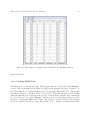
1
Habread User Manual
NCASI Statistics and Model Development Group
∗
Version 1 May 10, 2005
Abstract
Converting data to new formats can be a laborious task. Forest harvest scheduling
is a data intensive activity that has given rise to complex matrix generators for creating
input to Linear Program solvers. HabRead is a program that helps you convert data
in Linear Program MPS format into files that Habplan can read. The purpose is to
harness the years of development that went into the matrix generator so that users can
add Habplan to their suite of landscape planning tools.
∗
NCASI: http://ncasi.uml.edu/
1
Habread User Manual Draft: Do not distribute
1
Contents
1
Introduction
2 Habplan and Linear Programming Overview
4
4
2.1
Metropolis algorithm . . . . . . . . . . . . . . . . . . . . . . . . . . . . . . .
5
2.2
LP formulation . . . . . . . . . . . . . . . . . . . . . . . . . . . . . . . . . .
6
2.3
How does HabRead deconstruct the MPS file? . . . . . . . . . . . . . . . . .
9
2.4
Comments on Regime Naming Conventions . . . . . . . . . . . . . . . . . . .
10
3 How to Use HabRead
3.1
3.2
3.3
10
Example 1: Polygon/Regime Decision Variables Separated by a Character .
11
3.1.1
Creating the BIO2 data . . . . . . . . . . . . . . . . . . . . . . . . .
11
3.1.2
Creating FLOW data . . . . . . . . . . . . . . . . . . . . . . . . . . .
13
3.1.3
Outputting Results to Habplan . . . . . . . . . . . . . . . . . . . . .
15
Example 2: Polygon/Regime Decision Variables in Fixed-Width Fields - Expanding Management Units to Component Polygons . . . . . . . . . . . . .
16
3.2.1
Creating the BIO2 data . . . . . . . . . . . . . . . . . . . . . . . . .
17
3.2.2
Creating FLOW data . . . . . . . . . . . . . . . . . . . . . . . . . . .
18
3.2.3
Expanding Management Units . . . . . . . . . . . . . . . . . . . . . .
21
3.2.4
Outputting Results to Habplan . . . . . . . . . . . . . . . . . . . . .
23
Example 3: Polygon/Regime Decision Variables in Fixed-Width Fields - Converting from Per-Acre/Hectare Outputs to Whole-stand Outputs . . . . . . .
24
Habread User Manual Draft: Do not distribute
2
3.3.1
Creating the BIO2 data - and Converting to Whole-stand Outputs . .
24
3.3.2
Handling Spatial Issues For Pre-Cut Stands . . . . . . . . . . . . . .
26
3.3.3
Creating FLOW Data . . . . . . . . . . . . . . . . . . . . . . . . . .
28
3.3.4
Outputting Results to Habplan . . . . . . . . . . . . . . . . . . . . .
29
4 Habplan Data Formats
29
4.1
Flow Data . . . . . . . . . . . . . . . . . . . . . . . . . . . . . . . . . . . .
30
4.2
Biological Type II Data . . . . . . . . . . . . . . . . . . . . . . . . . . . . .
32
4.3
Comments on Preparing Input Data . . . . . . . . . . . . . . . . . . . . . .
32
5
Installing the Program
33
6
Known Bugs
35
7
Future Directions
35
8 APPENDIX: Background on Harvest Scheduling
8.1
Solving the Harvest Scheduling Problem . . . . . . . . . . . . . . . . . . . .
35
36
List of Figures
1
Example of an LP Tableau . . . . . . . . . . . . . . . . . . . . . . . . . . . .
6
2
Input the MPS data . . . . . . . . . . . . . . . . . . . . . . . . . . . . . . .
11
3
Create the BIO2 Table . . . . . . . . . . . . . . . . . . . . . . . . . . . . . .
12
Habread User Manual Draft: Do not distribute
3
4
Translating Polygon and Regime Names . . . . . . . . . . . . . . . . . . . .
13
5
Generating Flow Data . . . . . . . . . . . . . . . . . . . . . . . . . . . . . .
15
6
Checking for Consistency of Polygon Names . . . . . . . . . . . . . . . . . .
16
7
Reading the MPS file . . . . . . . . . . . . . . . . . . . . . . . . . . . . . . .
17
8
BIO2 Table . . . . . . . . . . . . . . . . . . . . . . . . . . . . . . . . . . . .
18
9
Flow1 Make Tool and Flow1 Table . . . . . . . . . . . . . . . . . . . . . . .
19
10
Flow2 Table for controlling clearcut acres . . . . . . . . . . . . . . . . . . . .
20
11
Flow3 Table for controlling regenerated acres . . . . . . . . . . . . . . . . . .
20
12
Flow4 Table for controlling thinned acres . . . . . . . . . . . . . . . . . . . .
21
13
Before Expanding Management Units to Component Polygons . . . . . . . .
22
14
After Expanding Management Units to Component Polygons . . . . . . . . .
22
15
MPS Read Tool . . . . . . . . . . . . . . . . . . . . . . . . . . . . . . . . . .
24
16
Before Converting Outputs to Whole-stand Values . . . . . . . . . . . . . . .
25
17
After Converting Outputs to Whole-stand Values . . . . . . . . . . . . . . .
25
18
Expand Units Form Setup for Pre-Cutting . . . . . . . . . . . . . . . . . . .
27
19
Flow Data for a Stand Cut 1 Year Before the Planning Horizon . . . . . . .
28
20
Flow 1 Table for Controlling Clearcut Acres . . . . . . . . . . . . . . . . . .
29
List of Tables
1
Example of flow data . . . . . . . . . . . . . . . . . . . . . . . . . . . . . . .
31
Habread User Manual Draft: Do not distribute
1
4
Introduction
Foresters have traditionally used linear programming (LP) for harvest scheduling. Mathematical Programming System (MPS) format is commonly used for feeding data into an
LP solver. Many forestry organizations have developed sophisticated systems for generating
MPS files, since virtually all LP solvers can read this format. HabRead is designed to allow
these organizations to add Habplan to their arsenal of planning tools while continuing to use
legacy systems. HabRead provides a spreadsheet-like format that makes it relatively easy to
transform an MPS file into Habplan compatible format.
Habplan is based on a different solution algorithm and objective function than LP, so it
can not directly utilize all of the information that is embedded in MPS files. For example,
constraints on flows will not be used. However, much of the basic data can be transformed
into Habplan format. The objective function coefficients form the basis for Habplan’s BIO2
component. The data for various kinds of flows can also be utilized.
2
Habplan and Linear Programming Overview
Habplan uses what has been traditionally called a Model I formulation, which requires stand
specific information. Habplan solutions are integer, so only one regime can be assigned to
each stand for a particular management schedule. LP has no such constraint, and it is possible for a stand or management unit to be assigned in fractional parts to many regimes.
In effect, this gives LP more degrees of freedom for solving problems with competing constraints.The LP solution leaves the final decision about what to actually do in the forester’s
hands. However, Habplan does not eliminate the need for a forester’s expertise. Habplan
can provide multiple integer solutions and the forester can select among these alternatives.
A key point is that Habplan deals with whole-stand outputs, not per-acre values. If the
values in the MPS file are per-acre, then they need to be converted to whole-stand. You
will need to provide a file of stand sizes in order for HabRead to do this internally. The
mechanisms of this procedure will be dealt with later.
Another important point is that Habplan typically deals in annual increments or periods.
Often an LP planning horizon is broken down into 5 or 10 year periods. Furthermore, the
period length can vary. For example, the planning horizon might be broken into four 5-year
periods followed by four 10-year periods for a total horizon length of 60 years. Habplan
could handle 5 or 10 year periods, but the period length shouldn’t vary. When dealing with
Habread User Manual Draft: Do not distribute
5
spatial issues like block-size and green up windows, it is usually necessary to have annual
increments instead of multi-year planning periods.
The Habplan and LP objective functions are quite different, which is why Habplan can’t
utilize all of the data in an MPS file. The following subsections give a brief overview of the
Metropolis algorithm (MA) and the objective function that Habplan uses. There is also an
overview of the LP Model I formulation that is compatible with Habplan. Finally, there is a
discussion about how HabRead extracts data from an MPS file. See the Appendix for some
additional background on harvest scheduling and the Model I and Model II formulations.
2.1
Metropolis algorithm
The Metropolis formulation used here has been described elsewhere (Van Deusen, 1999,
2001). The first step is to select an initial schedule, possibly at random, which evolves at
each iteration. The schedule at iteration r is represented by the vector X r = xr1 , ..., xrN ,
where xri represents the regime assigned to polygon i at iteration r. Each iteration of the
algorithm creates a new and improved schedule that can be compared with other schedules
using an objective function E(X r ).
The overall objective function consists of a weighted sum of components, where each
component represents a particular sub-objective. The value of the objective function at
iteration r is
J
X
r
E(X ) =
wjr−1 Cj (X r )
(1)
j=1
wjr
where
is a weight determined from the iteration r schedule, and Cj (X r ) is the jth objective
function component evaluated at the rth schedule.
The Metropolis algorithm iteratively considers new proposal regimes as substitutes for the
current regime of each polygon. The proposal regime is immediately accepted if it improves
the overall schedule by decreasing the objective function (1). Proposals that are worse than
the current regime can still be accepted according to a computed probability. It is possible
to escape a solution region that represents a local minima by sometimes accepting changes
that don’t improve the objective function. This algorithm does not attempt to converge on a
single best solution by slowly adjusting a so-called temperature parameter as with simulated
annealing as presented by (Lockwood and Moore, 1993). Rather, the individual component
weights can be adjusted for finer control of convergence properties.
Habread User Manual Draft: Do not distribute
6
The objective function is a sum of components multiplied by weights. The components
of interest when using HabRead are FLOW and BIO2 components. FLOW components deal
with maintaining even flow of a particular quantity over time. BIO2 components allow you
to bias the results of a Habplan run to favor regimes with larger ranks. Typically, the ranking
is based on present net value, so regimes that make more money are favored. However, the
ranking could be based on habitat value as well.
2.2
LP formulation
A brief introduction to the type of LP formulation that is compatible with Habplan is useful.
For convenience, a simple LP example is summarized in the form of a tableau (Figure 1).
This example consists of: 4 decision variables, 1 flow component, and a planning period of
2 years. This simple LP problem will be referred to for explanation purposes.
Figure 1: Example of an LP Tableau
The linear programming algorithm is well known and is based on maximizing or minimizing an objective function subject to constraints. It is generally specified as:
M ax Z = cx
subject to
Ax ≤ r
x ≥ 0
where Z is the objective function value, c is a vector of coeffcients representing the contribution of the decision variables, x is a vector of decision variables, A is a matrix of
Habread User Manual Draft: Do not distribute
7
coefficients measuring the effect of the constraints on the decision variables, and r is a vector
of constraints.
The components of Figure 1 and their relation to the LP setup will be explained briefly,
row by row. In the first row (column labels), the decision variables, xij , represent the
proportion of polygon i that is assigned to regime j (correspond to x in the general LP
format). The variables defined as Fn Yt , are (F)low accounting variables, that represent the
volume flow of flow component n in (Y)ear t. The Row Type determines the sign of the
mathematical expression, where:
• E: equality
• L: less than or equal to
• G: greater than or equal to
The RHS (Right Hand Side) refers to the value of the right hand side of the mathematical
expression (corresponds to r in the general LP format).
The objective function coefficients (second row), c(xij ) (Figure 1), are taken directly from
the Bio2 file (correspond to c in the general LP format). The following is an example of
data from the Bio2 file upon which the example tableau (Figure 1) is based:
1
1
2
2
1
2
1
2
10
20
30
40
The numbers in the first column represent the polygon ID, the numbers in the second column
represent the regime assigned to the polygon, and the numbers in the third column represent
the contribution of each decision variable (c(xij )) to the objective function value. So, the
objective function for this example would read as follows:
Max Z = 10 x11 + 20 x12 + 30 x21 + 40 x22
Habread User Manual Draft: Do not distribute
8
The third and fourth rows in Figure 1 constitute the acreage constraints of the form:
Ji
X
xij = 1
i = 1, 2, 3, . . .
j=1
where Ji is the number of valid regimes for polygon i.
This set of constraints is imposed to keep LP from assigning more than 100% of the polygon
to its set of valid regimes. These constraints are named Pi , where i is the polygon number.
The fifth and sixth rows in Figure 1 constitute the flow accounting constraints, which
are included to allow LP to keep track of annual outputs of items such as clearcut acres and
wood flow. Thus, these are not constraints in the true sense of the word, but rather perform
a “summing” function. These constraints are of the form:
X
anj xij − Fn Yt = 0
∀ n, t
xij ∈n,t
where the relevant xij are those polygons and regimes that contribute to the output that is
being accounted for in year t and for flow component n, and the anj coefficients (correspond
to A in the general LP format) give the contribution of each polygon to summary variable
Fn Yt . These constraints are named Fn At , which refers to the (F)low (A)ccounting constraint
for flow component n in year t. The flow volumes (the anj values) associated with each
decision variable are taken from the associated Flow file. The following is an example of
data from the Flow file upon which the example tableau (Figure 1) is based:
1
1
2
2
1
2
1
2
1
2
1
2
100
200
150
200
The numbers in the first column represent the polygon ID, the numbers in the second column
represent the regime assigned to the polygon, the numbers in the third column represent
the year in which output occurred, and the numbers in the fourth column represent the
contribution of each decision variable to the flow volume of a given year (Fn Yt ).
The seventh and eighth rows in Figure 1 constitute the flow constraints, which are different from the flow accounting constraints. These constraints are imposed to control the
Habread User Manual Draft: Do not distribute
9
trend and variability of periodic flow, and have the following form:
Fn Yt+1 ≤ (1 + U )Fn Yt
(1 − L)Fn Yt ≤ Fn Yt+1
t = 1, . . . , T − 1
t = 1, . . . , T − 1
where U and L are user-defined upper and lower proportions to control the change in flow
from one time to the next.
2.3
How does HabRead deconstruct the MPS file?
HabRead can input an MPS file that is either in the traditional fixed field-width format or
in a more flexible variable field-width format. The variable format can have fields separated
by white-space, commas or tabs. The fixed field format usually forces the user to encode
the polygon names and regime names in order to stay within the limited field width. A
typical encoding scheme would be to code polygon 10001 with regime 128 as decision variable
10001128, because this fits into the 8 character field in the fixed format MPS file. HabRead
allows the user to provide a translation table to tanslate the coded polygon and regime
names back to something more readable before inputting them into Habplan. For example,
you might want to change polygon 10001 to District8-Stand1 and regime 128 to CC-2010.
The translation option will not work if your regime names are stand-dependent (see 2.4).
HabRead attempts to construct a Bio2 file for Habplan by pulling out the non-zero objective function coefficients from the MPS file (Figure 1). HabRead infers the polygon names
and regime names by looking at the names of the xij variables associated with these nonzero coefficients. HabRead assumes that variable names can be deconstructed to separate
polygon and regime names by following certain patterns. The 2 basic schemes that HabRead
uses are: 1) The Polygon/Regime name is separated by a special character, such as “$”, or
2) The first n characters give the polygon name and the rest give the regime name.
Likewise, HabRead attempts to construct a Flow file by looking for user specified Flow
prefixes. In this example (Figure 1) the prefix is “F1A” and HabRead assumes that rows
labeled “F1A1” contain flow values for period 1, “F1A2” has values for period 2, etc.
If your MPS file is constructed in a similar fashion, then HabRead should work for you.
Habread User Manual Draft: Do not distribute
2.4
10
Comments on Regime Naming Conventions
Habplan was developed with the implicit assumption that regime names have similar meaning
across stands, i.e. they are stand independent. For example, regimes called CC#1 and
CC#2 might mean to clearcut the stand in years 1 and 2. However, MPS files often use
random regime encodings such that regime X for stand i has no relationship to regime X
for stand j. Fortunately, most of the features in Habplan will work when regime names are
stand-dependent.
The following things won’t work in Habplan when regime names are stand dependent:
(1) The Spatial Model(SMOD) Component, (2) indicating “Not-Block” options for the Block
(BK) Component, and (3) indicating Block options for the CCFLOW Component. All of
these capabilities depend on regime naming to be stand independent. There seems to be
no work-around for the Spatial Model Component, but there is for the Block Component.
This work-around is made possible by the fact that many MPS files already have a clearcut
flow incorporated, i.e. there are decision variables that allow the LP formulation to place
constraints on the amount of clearcutting by period.
Go to the Habplan documentation for more information about Block components, but
a Block component has a parent Flow component from which it gets information about
when management activities occur. If no regimes are designated as “NotBlock”, then the
Block component assumes that all regimes contribute to block size. Therefore, simply let
the clearcut flow component be the parent of the block component and it will automatically
treat every parent action that produces non-zero output as a block creating action. This
will give the desired control of block sizes.
3
How to Use HabRead
The following examples will step you through the process of using HabRead. The first step
is to get HabRead installed and running on your computer as outlined in the installation
instructions 5. HabRead can help you set up special management units that consist of
multiple polygons. Each polygon in a unit is assigned the same management regime. This
capability is discussed at the end of example 2. HabRead also has the ability to convert
per-acre outputs to whole-stand outputs, assuming the necessary data is provided in the
form of a dbf file. This capability is discussed in example 3.
Habread User Manual Draft: Do not distribute
3.1
11
Example 1: Polygon/Regime Decision Variables Separated by
a Character
This mps datafile was generated by Habplan using the built in LpMPS capability. The mps
file comes with Habread and can be found in the Habread1/example/test directory. The
first step is to open the MPSReadTool (Figure 2), press the file button, then select the
habplan2LP.mps file in the test directory. Alternatively, you can abbreviate the path to files
that are in the Habread example directory so “test/habplan2LP.mps” is a sufficient path.
This file has polygon and regime names separated by a dollar sign, so be sure to check the
“Use Split Character” box.
Figure 2: Input the MPS data
3.1.1
Creating the BIO2 data
Now press the “BIO2” button to read the MPS file and create the BIO2 Table (Figure 3). At
this point you need to carefully examine the polygon and regime names in the BIO2 Table to
make sure that they are all correct. There is a selection tool that can be accessed under the
“Tools” menu on the BIO2 Table that will help you search for specific polygon and regime
names. You can delete multiple rows by selecting them and pushing the delete button on
the selection tool. A single row can be deleted by pushing the “row-” button on the BIO2
Table.
Regimes that represent doing nothing are important in Habplan, and we call them
“DoNothing regimes”. For example, Habplan might break up a large clearcut block by
assigning a DoNothing regime to one of the polygons. There is an “AddDoNothing” button
on the Bio2Table that helps you ensure that each polygon has a DoNothing regime assigned
to it. For this example, regime 1 is DoNothing. If you select the first row (polygon 1, regime
1) in the Bio2 Table, and press the “AddDoNothing” button, it will make sure that each
Habread User Manual Draft: Do not distribute
12
Figure 3: Create the BIO2 Table
polygon has a DoNothing regime. Normally, “DoNothings” won’t show up in the LP formulation because they have a zero objective function coefficient. We assigned a value of 1.0 for
this problem, so they showed up in the MPS file.
If your data has no DoNothing regimes, just insert a row at the top of the file (using
“row+”) and fill it in with the first polygon name and an appropriate regime name (like
“DN”) and give it a value of 0. Then hit the “AddDoNothing” button to add this regime to
all the other polygons.
The “Translate” button opens a tool(Figure 4) that allows you to input translation tables
to change the names of polygons and regimes to something more readable. These are simple
text files with 2 columns. The regime and the polygon translation files have the same
format. The first column gives the polygon or regime code and the second column gives the
new name. The columns are separated by spaces, commas or tabs. Just push the “Run”
button to perform the translation. The translation is applied to all Bio2 and Flow tables, so
Habread User Manual Draft: Do not distribute
13
you might want to save this for last. Also, be careful of running translations multiple times.
If any of the same names can appear in the left and right columns of the translation files,
repeated translations could lead to erroneous results.
Figure 4: Translating Polygon and Regime Names
Whenever you select “Exit” from the HabRead “File” menu, the current settings are
saved to a default location in the hbr subdirectory. You can also select “SaveSettings” to
save your settings to another location. When you restart HabRead, it automatically loads
the settings saved in the default location. Also, whenever you push the “Save” button on
the BIO2 or on a Flow table, the table is saved to the default location. Note that the “Edit”
menu for each table has an “UnDo” option, so you can recover if you make changes that are
incorrect.
3.1.2
Creating FLOW data
Some of the steps required to properly fill out a FLOW data table depend on having all of
the polygon names in the BIO2 table, so complete the BIO2 table before moving to a FLOW
tab. Notice that you can add and remove flow tabs by selecting the option under the “Flow”
menu. You are allowed to have from 1 to 99 flow tabs.
Begin by supplying the prefix of the flow accounting variable. This is based on the
assumption that your MPS file has accounting variables that provide the sum of each Flow
for each period in the planning horizon. For this MPS file, row names that begin with “F1A”
(Figure 1) contain Flow coefficients. F1A1 are year 1 coefficients and F1A2 are for year2,
etc. Type in the prefix in the Flow Tool (Figure 5) and press the “Generate” button to fill
Habread User Manual Draft: Do not distribute
14
in the Flow Table.
The flow table should contain all of the polygons and regimes that appear in the BIO2
Table. Usually the DoNothing regimes and maybe entire polygons won’t be obtainable from
the MPS Flow accounting variables. For example, if this Flow component is for pine, then
the hardwood polygons won’t be included in the table, since they aren’t involved in pine
accounting. However, Habplan wants all polygons and regimes to appear in each flow dataset.
If the BIO2 table had do-nothings added before reading the FLOW table, the do-nothings
will be automatically carried over to the FLOW table. In fact, any regimes that are in
BIO2 will be carried over to the FLOW table to ensure consistency. However, you can do a
consistency check to verify this.
Press the “Consistency” button on the FLOW Table to find out if there are mis-matches
between the BIO2 and this FLOW Table. If there are polygons that appear in the FLOW
table, but not in the BIO2 table, then you need to manually fix things. Usually you need
to delete the rows from the FLOW table that don’t show up in the BIO2 table. If there are
no miss-matches between the BIO2 and FLOW tables, then you are ready to write this data
out for Habplan use.
If polygons are missing from the FLOW table that appear in the BIO2 table, Habplan
will have problems. Fill in the missing polygons by pressing the “Fill” button on the FLOW
table. This will pull all polygons and regimes that appear in BIO2 into the FLOW table if
they aren’t already represented. They will be given a 0.0 output value that appears in year
1. Therefore, it won’t affect the schedule, but Habplan will be happy. Fill gives you some
summary (Fig 5) information that helps you assess the correctness of the FLOW table data.
The “Fill” step is needed because Habplan will only use regimes that appear in all
objective function components. Habplan assumes that regimes that don’t appear in all
components are disallowed. This was supposed to be a feature that allows you to change
allowed regimes when entering a new objective function component.
Finally, you should run a consistency check to ensure that the Flow and BIO2 tables
contain the same polygons. Habplan will abort if polygons aren’t consistent across all components. Press the consistency button and 2 tables will appear. One table gives the polygons
that appear in BIO2, but not in Flow. The other table gives polygons in Flow, but not in
BIO2. You should get the results in Figure (6), which indicate that there are no missings.
Inconsistencies must be dealt with. If there are polygon names that appear in the Flow
Table that don’t belong, then delete them. If names need to be added, then add them, etc.
Don’t ignore iconsistencies, because Habplan won’t accept the data.
Habread User Manual Draft: Do not distribute
15
Figure 5: Generating Flow Data
3.1.3
Outputting Results to Habplan
At this stage in HabRead development, you need to output each data table to a directory
where Habplan can access the files. Select “WriteData” under a table’s “File” menu to
output the data to an ascii file. Don’t use the option of including the column names in
the first row of the output file. This file can then be input directly to Habplan as either a
BIO2 component or a FLOW component. This is done by filling out an Edit Form for the
component in Habplan.
Habread User Manual Draft: Do not distribute
16
Figure 6: Checking for Consistency of Polygon Names
3.2
Example 2: Polygon/Regime Decision Variables in FixedWidth Fields - Expanding Management Units to Component
Polygons
The following example is based on data in which the polygon/regime name is combined into
a single variable name, e.g. X00062074 would be cutting unit 62, regime 74. In other words,
Habread User Manual Draft: Do not distribute
17
the first 6 characters of this combined variable name give the polygon name, and the rest
give the regime name. As for example 1, the first step is to open the MPSReadTool and
select the desired MPS file. The primary difference between examples 1 and 2, however, are
that the polygon/regime names are combined into a single variable for example 2, and are
not separated by a split character as in example 1. Therefore, one would not check the “Use
Split Character” box (Figure 7). Instead, one would leave the “Use Split Character” box
unchecked, and enter “6” into the “Polygon/Regime Split Column” box. This would ensure
that the first 6 characters of the polygon/regime name are assigned to the polygon name,
and the rest to the regime name.
Figure 7: Reading the MPS file
3.2.1
Creating the BIO2 data
Now, in order to read the MPS file and create the BIO2 Table (Figure 8), press the “BIO2”
button. After verifying that all the polygon and regime names are correct, and after deleting
any undesired rows, ensure that each polygon is assigned a DoNothing regime, as explained
in Example 1. Unlike Example 1, DoNothing regimes did not exist in the MPS file for this
example. Thus, one has to create a DoNothing regime by inserting a row at the top of the
BIO2 file (using “row+”), and filling it in with the first polygon name and a regime name,
“DN”. A value of 0 is assigned to this regime. Now hit the “AddDoNothing” button to add
a DoNothing regime to all the other polygons.
As discussed in Example 1, whenever you select “Exit” from the HabRead “File” menu,
the current settings are saved to a default location in the hbr subdirectory. You can also
select “SaveSettings” to save your settings to another location. When you restart HabRead,
it automatically loads the settings saved in the default location. Also, whenever you push
the “Save” button on the BIO2 or on a Flow table, the table is saved to the default location.
Note that the “Edit” menu for each table has an “UnDo” option, so you can recover if you
make changes that are incorrect.
Habread User Manual Draft: Do not distribute
18
Figure 8: BIO2 Table
The next step is to create the flow data.
3.2.2
Creating FLOW data
Using the “AddFlow” option under the HabRead “Flow” menu, add as many flow components (maximum of 99) as you need. So too, one can delete unneeded flow components using
the “RemoveFlow” option. For this example, we have chosen to include 4 flow components.
At the top of the HabRead window, click on the first flow tab (Flow 1). Now, assuming
that the MPS file has accounting variables that provide the sum of each Flow for each period
in the planning horizon, supply the prefix of the first flow accounting variable in the “Flow1
Make Tool” window (Figure 9). For this example, MNCFL is the prefix for the accounting
variable that sums cash flow per period in the planning horizon, e.g. MNCFL01 refers to
cash flow in period 1. Type “MNCFL” in the “Flow1 Make Tool” and press the “Generate”
button to fill in the Flow Table (Figure 9). Now, after conducting the “Consistency” and
Habread User Manual Draft: Do not distribute
19
“Fill” operations, as described in section 3.1.2, you are ready to click on the second flow
tab (Flow 2), and repeat this process for the Flow 2 component, and all the subsequent flow
components (Figures 10, 11 and 12).
The data is now ready to be output to files that will be readable by Habplan.
Figure 9: Flow1 Make Tool and Flow1 Table
Habread User Manual Draft: Do not distribute
Figure 10: Flow2 Table for controlling clearcut acres
Figure 11: Flow3 Table for controlling regenerated acres
20
Habread User Manual Draft: Do not distribute
21
Figure 12: Flow4 Table for controlling thinned acres
3.2.3
Expanding Management Units
MPS data often represent aggregations of stands into management or cutting units (MUs).
In other words, what has been previously called a polygon might actually be a MU consisting
of several polygons or stands. HabRead can help you split these MUs into their component
polygons. The following section is an extention of Example 2, in that it is based on the same
data, but we now assume that the MPS data represents MUs, and not separate polygons.
This is also the place where per acre values from the mps file can be expanded to per polygon
values, which is what Habplan requires.
In order to split the MUs into their component polygons, one has to provide a dbf file
that has the following columns: 1)Polygon, 2) Unit, and 3) Size. The names in the Unit
column should correspond to the names in the MPS file. The polygon names correspond to
the polygons that make up a unit. Therefore, there will be more polygons than units. The
size column gives the size (area) of each polygon. This is used to apportion the output for a
MU to its component polygons. If you also have a shapefile that goes with the dbf file, you
could then use Habgen to generate a file for controlling block size.
The first step is to read the mps file and create the BIO2 table as discussed previously.
Then press the “Expand” button on the bottom of the BIO2 Table. This will give you
Habread User Manual Draft: Do not distribute
22
something like what is shown in (Figure 13).
Figure 13: Before Expanding Management Units to Component Polygons
The next step is set the file name to your dbf file. Then press the “SetColumns” button
to select the column names that correspond to Polygon, Unit and Siz e. If these names are
in the dbf file, they will be located automatically. Then press the “Read”button to read
the dbf file. Finally, press the “Expand Units” button to start the process of replacing the
management units with their component polygons. This also apportions the output for the
unit among the polygons according to their sizes. After this the BIO2 Table should look
something like (Figure 14)
Figure 14: After Expanding Management Units to Component Polygons
Along with everything else, the expansion puts the polygons in BIO2 into the same order
as they appear in the dbf file. This is important if you have a shapefile and want to use it
with Habplan. Shapes in a shapefile must correspond to rows in the accompanying dbf file.
Polygons that appear in the dbf file, but don’t have a unit that appears in the BIO2
file are inserted into the expanded BIO2 file with only a “DO-Nothing” regime. This is
to maintain the one-to-one correspondence with a shapefile. Finally, units that have no
polygon members in the dbf file are tacked on to the bottom of the BIO2 data. This will
allow Habplan to utilize the shapefile and incorporates all of your management units. In an
Habread User Manual Draft: Do not distribute
23
ideal world, there would be a complete correspondence between the units in your dbf file and
the units in the mps file. HabRead tries to do something reasonable, even when things are
less than ideal. Note that you can select the “undo” option under the edit menu to return
to the original BIO2 table if necessary.
The next step would be to click on a flow tab and press the expand button at the bottom
of the Flow Table. This will expand the units in the Flow table to correspond to the expanded
BIO2 table. Note that you should create the Flow data from the mps file before expanding
the BIO2 Table. The Flow table is referring to the BIO2 Polygon (unit) names and regimes
as it reads the mps file. If you read the mps file after BIO2 has been expanded you’ll end
up with lots of meaningless “Do Nothing” regimes in the Flow table.
For very large problems, you may run out of memory on your computer if you try
to create more than one Flow component at a time. In this case, create the BIO2 component,
expand it, and then save the result for Habplan. Then click “undo” to return to the original
BIO2 table. Now go to the first Flow tab and read in a Flow component. Expand the Flow
data and save it. Then read in another Flow component into the first flow tab, expand it,
and save it. Repeat this process until all Flows have been read, expanded and saved. This
will allow you to handle larger problems than is possible if you read each flow into a separate
flow tab. In general, you need lots of RAM if you are working with large MPS files. For
example, if the MPS file has 10 million lines, you could use 2 Gigabytes of RAM.
You need a special file to get Habplan to enforce these management units by assigning
the same regime to each polygon in a unit. This unitFile can be created by pushing the save
button on the Expand Units Form. This will save a text file that has 3 columns, polygon,
unit and size. Point Habplan to this file so it knows what management units to enforce.
3.2.4
Outputting Results to Habplan
In order to output each data table to a directory where habplan can access the files, for
each table, select “Writedata” under the table’s “File” menu. Save the data to a designated
directory from where Habplan will read the files, and do not include the column names when
saving (when you press save, a window will pop up giving you the option to include or exclude
the column names). It is advisable to save each component with a clearly understandable file
name, e.g. save BIO2 data as bio2.data, and save cash flow data as MNCFL.data (specific
to this example). These files can now be input directly into Habplan. This is done by filling
out an “Edit Form” for the respective components in Habplan.
Habread User Manual Draft: Do not distribute
3.3
24
Example 3: Polygon/Regime Decision Variables in FixedWidth Fields - Converting from Per-Acre/Hectare Outputs
to Whole-stand Outputs
Similar to Example 2, the following example is based on data in which the polygon/regime
name is combined into a single variable name. However, for this example, only the first
5 characters of the combined variable name give the polygon name, with the remaining
characters giving the regime name. Therefore, after opening the MPSReadTool (Figure 15),
and entering the filepath to the desired MPS file, one would leave the “Use Split Character”
box unchecked, and enter “5” into the “Polygon/Regime Split Column” box. This would
ensure that the first 5 characters of the polygon/regime name are assigned to the polygon
name, and the rest to the regime name.
Figure 15: MPS Read Tool
3.3.1
Creating the BIO2 data - and Converting to Whole-stand Outputs
If we were to follow the same procedure, as laid out in Examples 1 and 2, to create the
BIO2 file, we would now press the “BIO2” button, and the resulting table would look like
the table shown in Figure 16. Note that, for this example, DoNothing regimes were included
in the MPS file as regime “9999”. Therefore, there is no need for us to manually insert
DoNothing regimes. Also, this example is different from the previous two in that we know
that the output values in the MPS file are per-acre outputs. Habplan, however, deals only
with whole-stand outputs. Therefore, before saving the BIO2 data, we need to convert
these per-acre outputs to whole-stand outputs. The “Expand Units” option discussed in the
previous example can be used for this purpose.
After reading the MPS file (by pressing the “BIO2” button), press the “Expand” button
on the bottom of the BIO2 Table. This will open up the same “Expand” window that was
Habread User Manual Draft: Do not distribute
25
Figure 16: Before Converting Outputs to Whole-stand Values
Figure 17: After Converting Outputs to Whole-stand Values
used in Example 2 to convert management units to component polygons. You will now
need to provide a dbf file that includes the following columns: 1) Polygon and 2) Units and
Habread User Manual Draft: Do not distribute
26
3) Size. Proceed by setting the filepath to your dbf file on the “Expand” window. Now
press the “SetColumns” button to select the column names that correspond to “Polygon”,
“Unit” and “Size”. If these selected column names are in the dbf file, they will be located
automatically. Next, press the “Read” button to read the dbf file. Now simply check the
“Per Polygon” option on the “Expand” window, and then press the “BIO2” button on the
“MPS Read Tool” to generate the BIO2 data from the mps file. Then press the “Expand
Units” button and the units will be split out into their component polygons and turned into
whole stand values at the same time as shown in Figure 17.
This process can also be used when you only want to expand the mps values into whole
stand values. In this case the “Polygon” and the “Unit” variables should be set to the same
column in the dbf file. This particular dbf column should correspond to the names for the
stands in the mps file.
3.3.2
Handling Spatial Issues For Pre-Cut Stands
The beginning of a planning horizon is usually designated as year 1 in Habplan. However,
there will almost always be “pre-cut” stands that were cut 1, 2 or more years before the start
of the planning horizon. These stands will contribute to blocksizes in the first few years of
the planning horizon (until they green-up) and should be accounted for.
Habplan provides two ways to do this:
1. Start the planning horizon several years ahead of the current year.
2. Designate pre-cut years in a flow file as negative numbers.
The first method requires you to designate the early years of the planning horizon as
“byGone” on the Habplan Flow Edit Form. The regimes that were actually applied are
supplied for the stands in the byGone years. Habplan makes no effort to schedule things in
these byGone years, since they are in fact already scheduled.
The second approach may often be easier to implement and Habread can help you. The
idea is to create a Flow dataset that has years when precutting occurred designated by 1=”1 year before the start of the planning horizon”, -2=”2 years before”, etc. In order to
do this, there must be 2 additional columns in the polygon dbf file. The first is the “PreCut
Indicator” column. This column will contain a symbol, such as “Y” to indicate that this
Habread User Manual Draft: Do not distribute
27
polygon or stand was pre-cut. The second column is the “PreCut Year” column which gives
the period when the pre-cutting occurred relative to planning period 1. For example, a 0
means it occurred in period 0, -1 in period -1, and 1 would mean in period 1. There is also
a space to give the Indicator and the first period of the planning horizon on the “Expand
Units” form(Figure 18).
Figure 18: Expand Units Form Setup for Pre-Cutting
There is a difference between the “PreCut Year” values in the dbf file and the precut
years that go into Habplan Flow data files. In Habplan, the precut value is a lag that is
interpreted relative to the beginning of the planning horizon. Therefore, -1 in the Flow data
is equivalent to a 0 in the dbf PreCut Year column when the first period for Habplan is 1.
When the first period of the planning horizon is 2, then a -1 in the Flow data means the
stand was precut in year 1. If you don’t want to use the precut feature in Habread, just set
the PreCut Indicator variable to “none” and Habread ignores precutting.
This is what (Figure 19) the Flow data might look like when precutting is implemented.
The stand was cut 1 year before the start of the planning horizon. It is available for cutting
again in planning horizon years 18, 19 or 20 It is important to note that this only effects
Block Components that are subcomponents of the Flow component that has precut lags in
its data. If the flow component will not have a Block component, then set the “PreCut
Indicator” variable to “none”. For example, if you have a flow component specifically for
clearcutting, then it is a likely candidate for a Block component and could handle precut
Habread User Manual Draft: Do not distribute
28
Figure 19: Flow Data for a Stand Cut 1 Year Before the Planning Horizon
stands in its data.
3.3.3
Creating FLOW Data
The next step is to create the flow data. Following the same procedure as laid out in Examples
1 and 2, click on the first flow tab (Flow 1), supply the flow prefix, and press “Generate” on
the “Flow Make Tool” to fill in the flow table. Note that the “Flow Make Tool” displays the
following words in red: “Result = MPS * Polygon Size”. This indicates that you are dealing
with data that has been converted from per-acre- to whole-stand -outputs, and occurs when
the “Per Polygon” box on the “Expand” window is checked (dealt with in the preceeding
section on “creating the BIO2 data”). If the “Per Polygon” box is not checked, the following
words are displayed in yellow on the “Flow Make Tool”: “Result = Untransformed MPS
Habread User Manual Draft: Do not distribute
29
data”. Now, after conducting the “Consistency” and “Fill” operations, you are ready to
click on the second flow tab (Flow 2), and repeat this process for the Flow 2 component, and
all the subsequent flow components. The data can now be output to files that are readable
by Habplan.
Habread User Manual Draft: Do not distribute
30
Figure 20: Flow 1 Table for Controlling Clearcut Acres
3.3.4
Outputting Results to Habplan
As for Examples 1 and 2, in order to output each data table (BIO2 and Flow tables) to a
directory where habplan can access the files, for each table, select “Writedata” under the
table’s “File” menu. Save the data to a designated directory from where Habplan will read
the files, and do not include the column names when saving (when you press save, a window
will pop up giving you the option to include or exclude the column names). These files
can now be input directly into Habplan. This is done by filling out an “Edit Form” for the
respective components in Habplan.
4
Habplan Data Formats
Some discussion follows about the data formats that Habplan uses. However, only the data
that can be garnered from MPS files is discussed. For example, Habplan also uses neighbor
data for controling block sizes, but that is discussed elsewhere.
Habread User Manual Draft: Do not distribute
4.1
31
Flow Data
Each flow component requires a data set. For each polygon, there is one row for each regime
that is allowed. A disallowed regime is simply not included in the data for the polygon, which
prevents that regime from ever being assigned to that polygon. For example, maybe you
can’t allow clearcutting for polygon 10 because it’s near a stream. Be careful with multiple
flows that each flow dataset contains all allowed regimes, even if some of the regimes produce
0 output for some of the flows.
A simple example of some flow data follows. Note that outputs are polygon totals, NOT
per-acre or per-hectare. For regimes with multiple output years, the format calls for entering
the years and then the outputs, so if polygon 2 had 2 years of output for option 3, you have:
2 3 yr1 yr2 out1 out2 . For the data depicted below, polygon 1 can only be assigned option
16, while polygon 2 could have options 1-8.
Habread User Manual Draft: Do not distribute
32
Table 1: Example of flow data
Poly ID
1
2
2
2
2
2
2
2
2
Regime ID
16
1
2
3
4
5
6
7
8
Year Output
0
0
1
179
2
187
3
196
4
204
5
210
6
216
7
222
8
228
In general, polygon id and regime id can be any arbitrary name. Instead of polygon 1,
regime 1, you could name it polygon P1 and regime R1, for example. However, using integer
regime values has some advantage, since the entry forms for some components allow you to
use notation like 1-15 to indicate regimes 1 through 15. Of course, this only works for integer
regime names. Don’t use regime 0. Regime 0 is used by the biological type 1 component to
indicate that data being input are not training data. Also, the output is an integer – it takes
much less memory to store integers than floating points.
Option 16 is a do-nothing option in the above dataset. Do nothing options are denoted
with year=0 and usually with output=0 . Year=0 indicates that this period of this option
does not contribute to blocksizes, and this will be auto-detected by the blocksize component
for this flow. Finally, remember that regimes can have variable numbers of output years.
For example, regime 1 may produce output in years 1 and 21, while regime 20 only produces
output in year 20. There is no requirement for the data input file to be rectangular for flow
components. If you like rectangular files, however, you could create extra dummy periods
for your regimes with year=0. For example, suppose regime 2 has a second dummy period
for polygon 1 as follows:
1 2 1 0 120 0
The first period has an output of 120 for year 1 and the second period has output 0 in
year 0.
Habread User Manual Draft: Do not distribute
4.2
33
Biological Type II Data
The Type II biological component allows the user to specify the relative ranking of each
regime for each stand. Suppose you want to bias Habplan toward assigning the regime that
produces the most PNV for each stand. Then you need to assign a ranking for each regime.
In situations where the information is available to use the Type 2 biological approach, it is
to be preferred over the type 1 method, since it provides the user with more control.
The data format for this component is very simple. The first column is polygon id#, the
second is the option and the last column is the rank. There is one row for each stand and
regime. The following data show a situation where stand 1 must be assigned to regime 2
(the only regime given), but stand 2 could be assigned to regimes 1-3 with regime 3 being
preferred. The size of the numbers is irrelevant, only the ranking is important. Therefore
ranks 1,2,3 give the same result as .1, 16, 37.
121
2 1 0.1
2 2 0.4
2 3 0.5
4.3
Comments on Preparing Input Data
This section includes discussion on naming regimes and the procedure to indicate the valid
regimes for individual polygons. Habplan is very flexible with regard to polygon and regime
names. You can basically use whatever names you have in your current database for the
polygons. Likewise, any regime name can be used, but give serious thought to naming
regimes so that it’s easy to interpret the output. Habplan has to work harder when there
are lots of regimes, so don’t create regimes that represent trivial variations. For example,
cutting in May shouldn’t be considered different from cutting in June. If 2 polygons are
going to be clearcut in 2010 as the only management activity, then they are managed under
the same regime. There should also be a do-nothing regime assigned to each polygon, unless
there is a good reason not to do so, e.g. , the polygon was already cut in a byGone year.
This allows Habplan flexibility in meeting your goals. For example, it may be impossible to
meet blocksize limits unless some polygons are assigned to the do-nothing option (more on
Habread User Manual Draft: Do not distribute
34
do-nothings in a few paragraphs)
Usually, each polygon has only a subset of regimes that are valid. Valid regimes are
indicated to Habplan by the way the flow and bio-2 datasets are constructed. Specifically,
only include lines in these datasets for valid regimes. Habplan checks all flow components
and bio-2 components to determine the valid regimes. If anything is included for a regime
in both the Bio-2 or Flow data, then Habplan assumes its a valid regime for that polygon.
If there are 10 regimes for polygon xyz in the flow data and 8 regimes in the bio-2 data,
then there are at most 8 valid regimes. If there is no overlap between the regimes included in
the bio-2 and the flow datasets, then you’ll get an error message like this ”no valid regimes
for polygon xyz”. This also implies that the valid regimes for a polygon can change when a
new component is added to the objective function. In fact, the new component could make
a polygon’s current regime invalid. When this happens Habplan will switch to a new valid
regime ASAP, but not instantly.
Do-nothing options are specified in the Flow components as contributing to year 0, or
alternatively as having 0 flow, or both. Note that a do-nothing in one flow component might
result in output for another flow component. For example, doing nothing relative to clearcutting could result in a flow of habitat. The do-nothing option must also appear in Bio-2
components in order for it to be valid for a polygon. This implies that it must be ranked
relative to the other regimes. Hopefully, you can think of a meaningful way to accomplish
this ranking. For example, you might decide that the regime that yields the lowest present
net value is equal to doing nothing, and rank them accordingly. A do-nothing indicated
by year 0 (in Flow) signals the blocksize components that this option doesn’t contribute to
blocks. If you want it to contribute to blocks, then you’d have to give the year when it
contributes even though the output may be zero. See the material on the Block Form for
more on indicating do-Nothing regimes.
5
Installing the Program
HabRead is written in Java to be compliant with Sun Microsystems Java Development Kit
Version 1.2 or higher, which can be downloaded (free) from http://java.sun.com/j2se/. As
this is written, the current version is JAVA 2 Platform, Standard Edition, v 1.5.*, also called
JAVA 5. You only need to install the Java Runtime Environment (JRE) to run HabRead.
However, you need the entire J2SE to be able to use the jar command mentioned below.
Note that the jar command seems to be identical to the unzip command which you may
Habread User Manual Draft: Do not distribute
35
already have. If you have unzip, then you only need the JRE.
HabRead is a standalone program. Java programs are often run as Applets in a web
browser. However, HabRead requires access to system resources like reading and writing
files, which is considered a security violation for Applets. HabRead will run under Linux,
Unix, Apple and Windows operating systems.
Installing the program involves picking a starting directory where you put the habplan?.jar file, and then typing:
• jar xvf habread?.jar
This will uncompress the files that are in a Java Archive (jar) file. The JAR utility comes
with the J2SE. (If you only want to download the JRE, you should be able to unzip the jar
file using the PKUNZIP utility). You will now have a directory called HabRead1. Now type
the following:
• cd Habread?
• java Habread?
After a few seconds, Habread should appear on your screen. If you add the HabRead?
directory to your CLASSPATH, you can run HabRead from any location in your directory
structure. You had to deal with CLASSPATH when you installed the Jave J2SE, so it won’t
be explained again here. Make sure the bin directory for the J2SE is in your path so your
machine can find the java compiler. If you get the error that HabRead1.class isn’t found and
you executed the command ”java HabRead1” from within the Habread1 directory, then there
is probably a CLASSPATH variable set on your machine that doesn’t allow java to search
the current directory. If that happens, try executing like this: ”java -classpath . Habread1”,
where the ”.” tells java to look in the current directory.
It may be convenient to create a desktop shortcut for HabRead. If operating on Windows,
do the following:
• Open Wordpad and type the following command line:
java -mx256m -classpath . Habread1
Habread User Manual Draft: Do not distribute
36
• Under the Habread1 directory, save this as a text only “bat” file, e.g. h.bat.
• Now right click your mouse. Select “New” and “Shortcut”. Input the full file pathname
for the “h.bat” file, and follow the rest of the instructions, as laid out in Windows.
You may want to name the icon “Habread”.
• Once you have created this shortcut, in order to prevent the Dos Window opening each
time you open HabRead, right click on the HabRead icon. Click on “Properties”, then
“Shortcut”, and then under “Run”, select “Minimize”.
Now, to open HabRead, simply double click on the HabRead shortcut.
Note that the java interpreter allocates 16 MB of RAM by default. To run big problems,
get more RAM by starting HabRead like this: java -mx256m Habread?. This would allow
for 256 MegaBytes. It is wise to make this number as large as your computer will allow, i.e.
java -mx2000m Habread1 will give 2 GigaBytes of RAM.
6
Known Bugs
This section lists bugs that are known and not yet fixed. Users can provide information
on other bugs that they uncover. Please send email about bugs you find. 1) There are no
known bugs at this time.
7
Future Directions
1. Still working on finishing version 1.
8
APPENDIX: Background on Harvest Scheduling
The way in which a harvest scheduling problem is mathematically formulated is referred
to as the model of the problem. More specifically, the model refers to the way in which
the objective function and constraints are formulated. Two commonly spoken of models
are Model I and Model II formulations. The primary difference between the two is that
Habread User Manual Draft: Do not distribute
37
Model I choice variables are acres in a management unit, whereas Model II choice variables
are acres in an age class. In other words, a Model I formulation tracks each management
unit (e.g. forest stand) throughout its existence, and the identification of individual stands is
maintained. A Model II formulation tracks a given management unit until it is clearcut, after
which the new regenerating stand is merged with all other management units cut during the
same cutting period. These combined management units now, at age zero, become a new
management unit (age class), with a new identity. Thus, Model I looks at a management unit
and all the alternatives for managing it throughout a planning horizon (number of years in
the future for which a plan or projection is made), which is often multiple rotations. Model
II looks at an age class and the alternatives for managing that age class for a single rotation.
Habplan uses a Model I formulation. The primary advantage of using a Model I rather
than a Model II formulation is the ability to track all management units throughout their existence, which is a requirement when spatial constraints are included in a harvest scheduling
problem.
8.1
Solving the Harvest Scheduling Problem
As opposed to the model itself, the solution technique is the mathematical programming
technique that is used to solve the model. Two discrete catagories of solution algorithms are
1) optimization and 2) simulation.
Linear programming is a widely used mathematical programming tool for computing
optimal solutions to problems involving the allocation of scarce resources. This optimization
algorithm seeks to improve on simulation outputs by sorting through harvest schedules to
produce elevated combinations of objectives. This is done through the ranking of possible
harvest schedules using an objective function. LP was the first optimization method applied
to maximize harvestable volumes or Net Present Values (NPV), and has thus been around
for many years. The primary shortcoming of LP, however, is its limited ability to account
for spatial aspects of harvest scheduling. Thus, what LP suggests to be the optimal solution
usually turns out to be impossible in the real world.
With increasing emphasis placed on spatial concerns such as fragmentation and patch
size in forest management, and the continued introduction of new spatially-oriented environmental and social constraints, spatial simulation techniques continue to be developed.
These simulation algorithms mimic processes in harvest scheduling, seeking ultimately to
arrive at the same outcome that would occur had the situation been played out in real life.
Thus, these simulation algorithms do not offer one optimal solution, as does LP, but rather,
Habread User Manual Draft: Do not distribute
38
in principal, they compute a range of harvest schedules that are all feasible. At this stage,
we are not aware of any available simulation-based harvest-scheduling packages that report
multiple feasible solutions. Other harvest scheduling packages seem to simply converge on
the “best” solution. Habplan, however, does have the capability to report multiple feasible
solutions. Although these simulation techniques may not be capable of finding the perfectly
optimal solution, they are capable of finding near-optimal solutions, sometimes within a few
percent of the optimal.
Habplan uses a statistical simulation approach based on the Metropolis algorithm. It
also has limited built in LP capability, which is useful in that it allows the user to compare
the Metropolis algorithm solution to the non-spatial optimal solution. However, those who
are using HabRead already know what the LP solution is and want to find out what Habplan
can do.
Habread User Manual Draft: Do not distribute
39
References
Lockwood, C. and T. Moore (1993). Harvest scheduling with spatial constraints: a simulated
annealing approach. Canadian Journal of Forest Research 23, 468–478. 5
Van Deusen, P. C. (1999). Multiple solution harvest scheduling. Silva Fennica 33 (3), 207–
216. 5
Van Deusen, P. C. (2001). Scheduling spatial arrangement and harvest simultaneously. Silva
Fennica 35 (1), 85–92. 5