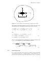
Download FRACOD Manual V11

2D
FRACOD
 A FRACOM Product
TWO DIMENSIONAL FRACTURE
PROPAGATION CODE
(VERSION 1.1)
USER’S MANUAL
Baotang Shen
FRACOM Ltd.
[email protected]
FRACOD User’s Manual
ABSTRACT
A two-dimensional boundary element code has been developed to
simulate fracture initiation and propagation in an elastic and isotropic rock
medium. The current version of the code is fully Window based and user
friendly. The code can simulate up to 10-15 non-symmetrical, and
randomly distributed fractures.
This manual provides: (a) the basic theoretical background of the
FRACOD code; and (b) a detailed instruction on how to use the code. A
number of simple examples are provided at the end of the report to
demonstrate the applicability of the code.
The current version of the FRACOD code was developed based on a
Ph.D. research (Shen, 1993). Further work on the code was conducted
during 1998-2001, supported by SKB, Fracom Ltd and Tekes. It was
designed to simulate fracture propagation in hard rocks.
i
FRACOD User’s Manual
TABLE OF CONTENTS
ABSTRACT
i
1
INTRODUCTION
1
2
THEORETICAL BACKGROUND
2
2.1
DISPLACEMENT DISCONTINUITY METHOD (DDM)
2
2.1.1
2.1.2
DISPLACEMENT DISCONTINUITY METHOD IN AN INFINITE SOLID
NUMERICAL PROCEDURE
2
3
2.2
2.3
2.4
2.5
SIMULATION OF ROCK DISCONTINUITIES
6
FRACTURE PROPAGATION CRITERION
8
DETERMINATION OF FRACTURE PROPAGATION USING
DDM
10
FRACTURE INITIATION CRITERION
11
3
CODE STRUCTURE
16
4
PREPARE INPUT FILE
19
5
CONDUCT AND MONITOR THE CALCULATION
24
REFERENCES
35
ACKNOWLEDGEMENTS
38
APPENDIX I – HOW TO USE THE PREPROCESSOR TO SET UP MODELS
39
APPENDIX II – VERIFICATION AND APPLICA-TION OF FRACOD
43
APENDIX III – DETERMINATION OF THE DIRECTION OF SHEAR
FRACTURES
69
ii
FRACOD User’s Manual
1
INTRODUCTION
Fracture propagation code (FRACOD) is a two-dimensional computer code
that was designed to simulate fracture initiation and propagation in elastic
and isotropic rock mediums. The code employs the Boundary Element
Method (BEM) principles and a newly proposed fracture propagation
criterion for detecting the possibility and the path of a fracture propagation,
Shen and Stephansson (1993).
The current version of the FRACOD code provides the basic functions
needed for studying rock fracture propagation in a rock mass subjected to
far-field stresses. The code is created for running on PCs with a MS
Windows 95/98/NT/2000 platform. It provides an easy-to-use user’s
interface that enables users to monitor and interrupt the calculation. It also
provides an independent pre-processor to help users in preparing the input
file for a given problem.
The capacity of the current version of the FRACOD code is limited to about
10-15 fractures, depending upon the complexity of the fracture system and
the excavation. As a general estimate, a fracture system with 10 nonsymmetrical fractures will requires about 24 hours of calculation on a
PC/400MHz to get a reasonably accurate prediction of fracture propagation.
This user’s manual provides some basic theoretical background of the code
in Chapters 2 and 3, and a detailed instruction on how to use the code in
Chapters 4 and 5. Appendix I describes a pre-processor of the FRACOD
code, while Appendix II gives ten simple application examples of using the
FRACOD code. For those who may be only interested in knowing how to
use the code rather than the theory, it is recommended to ignore Chapters 2
and 3 and start reading from Chapter 4.
1
FRACOD User’s Manual
2
THEORETICAL BACKGROUND
The FRACOD code is based on the Boundary Element Method principals. It
utilises the Displacement Discontinuity Method (DDM), one of the three
commonly used boundary element methods. In the FRACOD code, a newly
proposed fracture criterion, the modified G-criterion (Shen and
Stephansson, 1993), is incorporated into the numerical method for
simulating fracture propagation. This section describes in detail the
numerical method DDM as well as the modified G-criterion.
2.1
DISPLACEMENT DISCONTINUITY METHOD (DDM)
A crack or fracture has two surfaces or boundaries, one effectively
coinciding with the other. Conventional boundary element methods, such as
the Direct Integration Method, therefore become inefficient in simulating
this problem. The Displacement Discontinuity Method (DDM) was
developed by Crouch (1976) to cope with problems of this type. The DDM
is based on the analytical solution to the problem of a constant discontinuity
in displacement over a finite line segment in the x, y plane of an infinite and
elastic solid. Physically, one may imagine a displacement discontinuity as a
line crack whose opposing surfaces have been displaced relative to one
another (see Figure 2-1.)
2.1.1
Displacement Discontinuity Method in an infinite solid
The problem of a constant displacement discontinuity over a finite line
segment in the x, y plane of an infinite elastic solid is specified by the
condition that the displacements be continuous everywhere except over the
line segment in question. The line segment may be chosen to occupy a
certain portion of the x-axis, say the portion |x|≤a, y=0. If we consider this
segment to be a line crack, we can distinguish its two surfaces by saying that
one surfaces is on the positive side of y=0, denoted y=0+ , and the other is
on the negative side, denoted y=0- . In crossing from one side of the line
segment to the other, the displacement undergoes a constant specified
change in value Di = (Dx, Dy).
We will define the displacement discontinuity Di as the difference in
displacement between the two sides of the segment as follows:
D x = u x ( x ,0 − ) − u x ( x ,0 + )
D y = u y ( x ,0 − ) − u y ( x ,0 + )
2-1
Because ux and uy are positive in positive x and y co-ordinate direction, it
follows that the Dx and Dy are positive as illustrated in Figure 2-1.
2
FRACOD User’s Manual
y
+Dy
+Dx
x
2a
Figure 2-1. Constant displacement discontinuity components Dx and Dy.
The solution of the subject problem is given by Crouch (1976) and Crouch
and Starfield (1983). The displacement and stresses can be written as:
[
] [
]
u y = Dx [(1 − 2ν ) f , x − yf, xy ]+ D y [2(1 −ν ) f , y − yf, yy ]
u x = Dx 2(1 − ν ) f , y − yf, xx + D y − (1 − 2ν ) f , x − yf, xy
2-2
and
[
]
[
σ yy = 2GDx [− yf, xyy ]+ 2GD y [ f , yy − yf, yyy ]
σ xy = 2GDx [ f , yy + yf, yyy ]+ 2GD y [− yf, xyy ]
σ xx = 2GDx + 2 f, xy + yf, xyy + 2GD y f , yy + yf, yyy
]
2-3
where f,x represent the derivative of function f(x,y) against x, similarly as for
f,y, f,xy, f,xxy etc. Function f(x,y) in these equations is given by:
f ( x, y ) =
−1 
y
y
− arctan
)
y (arctan

4π (1 − ν ) 
x−a
x+a
− ( x − a ) ln
[( x − a)
2
]
+ y 2 + ( x + a ) ln
[( x + a)
2
]
+ y2 

2-4
2.1.2
Numerical procedure
For a crack of any shape, such as curved, we assume it can be represented
with sufficient accuracy by N straight segments, joined end by end. The
positions of the segments are specified with reference to the x, y co-ordinate
3
FRACOD User’s Manual
system shown in Figure 2-2. If the surface of the crack are subjected to
stress (for example, a uniform fluid pressure – p), they will displace relative
to one another. The displacement discontinuity method is a means of finding
a discrete approximation to the smooth distribution of relative displacement
that exits in reality. The discrete approximation is found with reference to
the N subdivisions of the crack depicted in Figure 2-2a. Each of the
subdivisions is a boundary element and represents an elemental
displacement discontinuity.
(a)
(b)
s
y
n
s
n
α
n=0+
N
j
j
2a
N
n=0-
(x,y)
Ds
j
j
x
Dn
i
2a
i
i
i
3
1 2
3
1 2
σs
σn
Figure 2-2. Representation of a crack by N elemental displacement
discontinuities.
The elemental displacement discontinuities are defined with respect to the
local co-ordinates s and n indicated in Figure 2-2. Figure 2-2b depicts a
single elemental displacement discontinuity at jth segment of the crack. The
components of discontinuity in the s and n directions at this segment are
j
j
donated as D s and D n . These quantities are defined as follows:
j
j
j
j
j
−
n
j
+
n
Ds = u s− − u s+
Dn = u − u
2-5
j
j
In these definitions, u s and u n refer to the shear (s) and normal (n)
displacement of the jth segment of the crack. The superscripts ‘+’ and ‘-‘
denote the positive and negative surfaces of the crack with respect to local
co-ordinate n.
j
j
The local displacements u s and u n form the two components of a vector.
They are positive in the positive direction of s and n, irrespective of whether
we are considering the positive or negative surface of the crack. As a
consequence, it follows from Equation 2-5 that the normal component of
4
FRACOD User’s Manual
j
displacement discontinuity D n is positive if the two surfaces of the crack
j
displace toward one another. Similarly, the shear component D s is positive
if the positive surface of the crack moves to the left with respect to the
negative surface.
The effects of a single elemental displacement discontinuity on the
displacements and stresses at an arbitrary point in the infinite solid can be
computed from the results for section 2.1.1, provided we suitably transform
the equations to account for the position and orientation of the line segment
in question. In particular, the shear and normal stresses at the midpoint of
the ith element in Figure 2-2b can be expressed in terms of the displacement
discontinuity components at the jth element as follows:

i=1 to N
ij
j
ij
j 
i
σ n = Ans Ds + Ann Dn 
i
ij
j
ij
j
σ s = Ass Ds + Asn Dn 
2-6
ij
where A ss ,etc., are the boundary influence coefficients for the stresses. The
ij
coefficient A ns , for example, gives the normal stress at the midpoint of the
j
ith element (i.e. σ n ) due to a constant unit shear displacement discontinuity
j
over the jth element (i.e. D s =1).
Returning now to the crack problem depicted in Figure 2-2b, we place an
elemental displacement discontinuity at each of the N segments along the
crack and write, from Equation 2-6,
i
N
ij
j
N
ij
j

σ s = ∑ Ass Ds + ∑ Asn Dn 

 i=1 to N
i
σ n = ∑ Ans Ds + ∑ Ann Dn 

j =1
j =1
j =1
N
j =1
ij
j
N
ij
2-7
j
j
j
If we specify the values of the stress σ s and σ n for each element of the
crack, then Equation 2-7 is a system of 2N simultaneous linear equations in
2N unknowns, namely the elemental displacement discontinuity components
j
j
D s and D n . We can find the displacements and stresses at designated
points in the body by using the principle of superposition. In particular, the
displacements along the crack of Figure 2-2a are given by expressions of the
form
5
FRACOD User’s Manual
j
j 
i
N ij
N ij
u s = ∑ Bss Ds + ∑ Bsn Dn 
j =1
j =1

 i=1 to N
j
j
i
N ij
N ij

u n = ∑ Bns Ds + ∑ Bnn Dn 
j =1
j =1

2-8
ij
where B ss , etc., are the boundary influence coefficients for the
displacements. The displacements are discontinuous when passing from one
side of the jth element to the other, so we must distinguish between these
two sides when computing the influence coefficients in Equation 2-8. The
diagonal terms of the influence coefficients in these equations have the
values
ij
ij
ij
ij
Bsn = Bns = 0
Bss = Bnn
2-9
1
1
= − (n → 0 + );+ (n → 0 − );
2
2
The remaining coefficients (i.e. the ones for which i≠j) are continuous and
they can be obtained by using Equations 2-1, 2-2 and 2-3 in Section 2.1.1.
i
Displacements u s
i
and u n
i
in Equation 2-8 will exhibit constant
i
discontinuities D s and D n , as required.
2.2
SIMULATION OF ROCK DISCONTINUITIES
For a rock discontinuity (crack, joint, etc.) in an infinite elastic rock mass,
the system of governing equations 2-7 can be written as
N
i
ij
N
j
ij
j
i

σ s = ∑ Ass Ds + ∑ Asn Dn − (σ s ) 0 

 i=1 to N
N
N
ij
j
ij
j
i
i
σ n = ∑ Ans Ds + ∑ Ann Dn − (σ n ) 0 

j =1
j =1
j =1
j =1
i
2-10
i
where σ s and σ n represent the shear and normal stresses of the ith element
i
i
respectively; (σ s ) 0 , (σ n ) 0 are the far-field stresses transformed in the crack
ij
ij
shear and normal directions. Ass , ... , Ann are the influence coefficients, and
j
j
Ds , Dn represent displacement discontinuities of jth element which are
unknowns in the system of equations.
A rock discontinuity has three states: open, in elastic contact or sliding. The
system of governing equations 2-10, developed for an open crack, can be
6
FRACOD User’s Manual
easily extended to the case for cracks in contact and sliding. For different
crack states, their system of governing equations can be rewritten in the
i
i
following ways, depending on the shear and normal stresses ( σ s and σ n )
of the crack.
i
i
• For an open crack σ s = σ n = 0, therefore the system of governing
equations 2-10 can be rewritten as:
N
i
ij
N
j
ij
j
i

σ s = 0 = ∑ Ass Ds + ∑ Asn Dn − (σ s ) 0 

 i=1 to N
σ n = 0 = ∑ Ans Ds + ∑ Ann Dn − (σ n ) 0 

j =1
j =1
j =1
N
i
j =1
ij
N
j
ij
j
2-11
i
i
When the two crack surfaces are in elastic contact, the magnitude of σ s
•
i
and σ n will depend on the crack stiffness (Ks, Kn) and the displacement
j
j
discontinuities ( Ds , Dn )
i
i
i
i
σ s = K s Ds
2-12
σ n = K n Dn
where Ks and Kn are the crack shear and normal stiffness, respectively.
Substituting Equation 2-12 into Equation 2-10 and carrying out the simple
mathematical manipulation, the system of governing equations then
becomes:
N
N
ij
j
ij
j
i
i 
0 = ∑ Ass Ds + ∑ Asn Dn − (σ s ) 0 − K s Ds 
j =1
j =1

 i=1 to N
N
N
ij
j
ij
j
i
i
0 = ∑ Ans Ds + ∑ Ann Dn − (σ n ) 0 − K n Dn 

j =1
j =1
•
2-13
For a crack with its surfaces sliding
i
i
σ n = K n Dn
i
i
i
σ s = ± σ n tan φ = ± K n Dn tan φ
2-14
i
where φ is the friction angle of the crack surfaces. The sign of σ s depends
on the sliding direction. Consequently, the system of equations 2-10 can be
presented as:
7
FRACOD User’s Manual
N
N
ij
j
ij
j
i
i

0 = ∑ Ass Ds + ∑ Asn Dn − (σ s )0 ± K n Dn tan φ 
j =1
j =1

 i=1 to N
N
N
ij
j
ij
j
i
i

0 = ∑ Ans Ds + ∑ Ann Dn − (σ n )0 − K n Dn

j =1
j =1
j
2-15
j
The displacement discontinuities ( Ds , Dn ) of the crack are obtained by
solving the system of governing equations using conventional numerical
techniques, e.g. Gauss elimination method. If the crack is open the stresses
i
i
( σ s , σ n ) on the crack surfaces are zero, otherwise if the crack is in contact
or sliding, they can be calculated by Equations 2-12 or 2-14.
The state of each crack (joint) element can be determined using the MohrCoulomb failure criterion:
(1) open joint:
(2) elastic joint:
(3) sliding joint:
σn > 0
σn < 0, |σs| < c + |σn|tanφ
σn < 0, |σs| ≥ c + |σn|tanφ
where a compressive stress is taken to be negative and c is cohesion. If the
joint has experienced sliding, c = 0.
2.3
FRACTURE PROPAGATION CRITERION
In modelling fracture propagation in rock masses where both tensile and
shear failure are common, a fracture criterion for predicting both mode I and
mode II fracture propagation is needed. The exiting fracture criteria in the
macro-approach can be classified into two groups: the principal stress
(strain)-based criteria and the energy-based criteria. The first group consists
of the Maximum Principal Stress Criterion and the Maximum Principal
Strain Criterion; the second group includes the Maximum Strain Energy
Release Rate Criterion (G-criterion) and the Minimum Strain Energy
Density Criterion (S-criterion). The principal stress (strain)-based criteria
are only applicable to the mode I fracture propagation which relies on the
principal tensile stress (strain). To be applied for the mode II propagation, a
fracture criterion has to consider not only the principal stress (strain) but
also the shear stress (strain). From this point of view, the energy based
criteria seem to be applicable for both mode I and II propagation because
the strain energy in the vicinity of a fracture tip is related to all the
components of stress and strain.
Both the G-criterion and the S-criterion have been examined for application
to the mode I and mode II propagation (Shen and Stephansson, 1993), and
neither of them is directly suitable. In a study by Shen and Stephansson
(1993) the original G-criterion has been improved and extended. The
8
FRACOD User’s Manual
original G-criterion states that when the strain energy release rate in the
direction of the maximum G-value reaches the critical value Gc, the fracture
tip will propagate in that direction. It does not distinguish between mode I
and mode II fracture toughness of energy (GIc and GIIc). In fact, for themost
of the engineering materials, the mode II fracture toughness is much higher
than the mode I toughness due to the differences in the failure mechanism.
In rocks, for instance, GIIc is found in laboratory scale to be at least two
orders of magnitude higher than GIc (Li, 1991). Applied to the mixed mode I
and mode II fracture propagation, the G-criterion is difficult to use since the
critical value Gc must be carefully chosen between GIc and GIIc.
A modified G-criterion, namely the F-criterion, was proposed (Shen and
Stephansson, 1993). Using the F-criterion the resultant strain energy release
rate (G) at a fracture tip is divided into two parts, one due to mode I
deformation (GI) and one due to mode II deformation (GII). Then the sum of
their normalized values is used to determine the failure load and its
direction. GI and GII can be expressed as follows (Figure 2-3): if a fracture
grows an unit length in an arbitrary direction and the new fracture opens
without any surface shear dislocation, the strain energy loss in the
surrounding body due to the fracture growth is GI. Similarly, if the new
fracture has only a surface shear dislocation, the strain energy loss is GII.
The principles of the F-criterion can be stated as follows:
G
Original
surface
New
surface
(a)
=
GI
+
GII
Growth
(b)
(c)
Figure 2-3. Definition of GI and GII for fracture growth. (a) G, the growth
has both open and shear displacement; (b) GI, the growth has only open
displacement; (c) GII, the growth has only shear displacement.
(1). In an arbitrary direction (θ) at a fracture tip there exists a F-value, which
is calculated by
F (θ) =
GI (θ ) GII (θ )
+
GIc
GIIc
2-16
(2). The possible direction of propagation of the fracture tip is the direction
(θ=θ0) for which the F-value reaches its maximum.
F (θ)
θ =θ0
= max .
2-17
(3). When the maximum F-value reaches 1.0, the fracture tip will propagate,
i.e.
9
FRACOD User’s Manual
F (θ ) θ =θ 0 = 1.0
2-18
The F-criterion is actually a more general form of the G-criterion and it
allows us to consider mode I and mode II propagation simultaneously. In
most cases, the F-value reaches its peak either in the direction of maximum
tension (GIc = maximum while GIIc=0) or in the direction of maximum
shearing (GIIc = maximum while GIc=0). This means that a fracture
propagation of a finite length (the length of an element, for instance) is
either pure mode I or pure mode II. However, the fracture growth may
socialite between mode I and mode II during an ongoing process of
propagation, and hence form a path which exhibits the mixed mode failure
in general.
2.4
DETERMINATION
USING DDM
OF
FRACTURE
PROPAGATION
The key step in using the F-criterion is to determine the strain energy release
rate of mode I (GI) and mode II (GII) at a given fracture tip. As GI and GII
are only the special cases of G, the problem is then how to use DDM to
calculate the strain energy release rate G.
The G-value, by definition, is the change of the strain energy in a linear
elastic body when the crack has grown one unit of length. Therefore, to
obtain the G-value the strain energy must first be estimated.
By definition, the strain energy, W, in a linear elastic body is
W = ∫∫∫
1
σ ε dV .
v 2 ij ij
2-19
where σij and εij are the stress and strain tensors, and V is the volume of the
body. The strain energy can also be calculated from the stresses and
displacements along its boundary
W=
1
∫ (σ s u s + σ n u n )ds
2 s
2-20
where σs,σn, us, un are the stresses and displacements in tangential and
normal direction along the boundary of the elastic body. Applying Equation
2-20 to the crack system in an infinite body with far-field stresses in the
shear and normal direction of the crack, (σs)0 and (σn)0, the strain energy, W,
in the infinite elastic body is
W=
1 a
∫ ( σ s − ( σ s ) 0 ) Ds + ( σ n − ( σ n ) 0 ) Dn da
2 0
2-21
10
FRACOD User’s Manual
where a is the crack length, Ds is the shear displacement discontinuity and
Dn is the normal displacement discontinuity of the crack. When DDM is
used to calculate the stresses and displacement discontinuities of the crack,
the strain energy can also be written in terms of the element length (ai) and
the stresses and displacement discontinuities of the ith element of the crack.
W ≈
i
i
i
i
i
i
i
i
1
(a(σ s − (σ s ) 0 ) Ds + a(σ n − (σ n ) 0 ) Dn )
∑
2 i
2-22
The G-value can be estimated by
G (θ) =
W ( a + ∆a ) − W ( a )
∂W
≈
∂a
∆a
2-23
where W(a) is the strain energy governed by the original crack while W(a+∆
a) is the strain energy governed by both the original crack, a, and its small
extension, ∆a (Figure 2-4). In Figure 2-4, a 'fictitious' element is introduced
to the tip of the original crack with the length ∆a in the direction θ. Both
W(a) and W(a+∆a) can be determined easily by directly using DDM and
Equation 2-23.
Crack
∆a θ
a
Figure 2-4. Fictitious crack increment ∆a in direction θ with respect to the
initial crack orientation.
In the above calculation, if we restrict numerically the shear displacement of
the “fictitious” element to zero, the result obtained using Equation 2-23 will
be GI(θ). Similarly, if we restrict the normal displacement of the “fictitious”
element to zero, the result obtained will be GII(θ). After obtaining both GI(θ)
and GII(θ), the F-value in Equation 2-16 can be calculated using the given
fracture toughness values GIc and GIIc of a given rock type.
2.5
FRACTURE INITIATION CRITERION
In addition to the propagation of existing fractures, new fractures (cracks)
may initiate at the boundaries or in the intact rock. This section describes
the criteria used to detect fracture initiation.
Fracture initiation in intact rock
11
FRACOD User’s Manual
Fracture initiation is a complicated process. It often starts from microcrack
formation. The microcracks coalesce and finally form macro-fractures.
Because the FRACOD code is designed to simulate the fracturing process in
macro-scale only, we ignore the process of microcrack formation. Rather,
we will only focus on when and whether a macro-fracture will form at a
given location with a given stress state.
The FRACOD code considers the intact rock as a flawless and
homogeneous medium. Therefore, any fracture initiation from such a
medium represents a localised failure of the intact rock. The localised
failure can be predicted by an existing failure criterion, e.g. Mohr-Coulomb
criterion. Other criteria widely used in rock mechanics and rock engineering
can also be used, such as Hoek-Brown criterion etc.
A rock failure can be caused by tension or shear. Hence, a fracture initiation
can be formed due to tension or shear. For tensile fracture initiation, the
tensile failure criterion is used in FRACOD, i.e. when the tensile stress at a
given point of the intact rock exceeds the tensile strength of the intact rock,
a new rock fracture will be generated in the direction perpendicular to the
tensile stress (Figure 2-5)
Critical stress of fracture initiation in tension:
σtensile ≥ σt
Direction of fracture initiation in tension:
θit = θ(σtensile)+π/2
where σtensile is the principal tensile stress at a given point, σt is the tensile
strength of the intact rock, θit is the direction of the fracture initiation in
tension, and θ(σtensile) is the direction of the tensile stress.
The length of the newly generated fracture is determined by the spacing of
the grid points used in the intact rock. In the current FRACOD version, it is
equal to the grid point spacing in the initiation direction. The less the grid
point spacing, the shorter the new fracture. However, the closer the grid
points, the less different the stresses at the adjacent grid points, and hence
the more likely a fracture initiation occurs in the adjacent grid points
simultaneously. The newly formed short fractures link with each other to
form a longer fracture. This mechanism reduces the sensitivity of the
modelling results to the grid point spacing.
12
FRACOD User’s Manual
New fracture
Tensile stress
Shear stress
Grid point
New fracture
Figure 2-5. Fracture initiation in tension or shear in intact rock.
For a shear fracture initiation, the Mohr-Coulomb failure criterion is used in
FRACOD, i.e. when the shear stress at a given point of the intact rock
exceeds the shear strength of the intact rock, a new rock fracture will be
generated (Figure 2-5)
Critical stress of fracture initiation in shear:
σshear ≥ σntan(φ)+c
Direction of fracture initiation in shear:
θis = φ/2+π/4
where σtensile is the shear stress in the direction of θis, σn is the normal stress
to the shear failure plane, φ is the internal friction angle of intact rock, c is
the cohesion, and θis is the direction of potential shear failure, which is
measured from the direction of the minimum principal stress.
Because there are always two symmetric shear failure planes at any given
point, two fractures are added in the model whenever a shear failure is
detected. Often one of the two fractures will propagate predominately in
later simulation of fracture propagation.
The length of the shear fracture initiation depends upon the spacing of the
grid points, as discussed above for the tensile fracture initiation.
Fracture initiation at boundaries
13
FRACOD User’s Manual
Fracture initiation at a boundary is not as a straight forward task as that in
intact rock. Because the boundary may be a straight boundary, a curved
boundary, or a boundary with sharp corners, significantly stress
concentration may occur at the boundary. Recent study by Shen and Rinne
(2001) has highlighted the complexity of the fracture initiation at
boundaries. The initiation criteria suggested by Shen and Rinne (2001) may
be suitable for the cases studied but not universally for all cases. There is no
simple and yet theoretically sound methods for the prediction of fracture
initiation from boundaries.
To enable the simulation of fracture propagation at boundary using
FRACOD, an alternative approach is taken. Instead of directly predicting
the fracture initiation from a boundary, we examine the fracture initiation
from the intact rock very close to the boundary, using the intact rock failure
criteria as discussed before. Once an intact rock failure is detected, a
fracture initiation is predicted to occur in the intact rock close to the
boundary. FRACOD then detects whether the newly formed fracture will
link to the boundary by using the fracture propagation functions. This
treatment fully utilises the advantage of the fracture propagation functions
built in the code and overcomes the lack of effective methods in handling
fracture initiation from the boundary.
New grid points are arranged in the intact rock along the boundary (Figure
2-6). They are set to be at a distance of one element away from the
boundary since the constant DDM method does not give accurate results
very close to the element. The grid points are effectively treated to be the
same as other grid points in the intact rock, and the same procedure is used
to detect any possible fracture initiation from these grid points. If a fracture
initiation is predicted from any of the grid points close to the boundaries, a
new fracture is created at the grid point in the direction of failure. The
length of the fracture is a half of the length of the nearest boundary element.
The code then detects whether the fracture will propagate to the boundary. If
yes, the fracture will link to the boundary and effectively form a fracture
initiation from the boundary.
Grid point
Fracture
initiation
Fracture
propagation
Boundary
Figure 2.6. Modelling process of a fracture initiation from boundary.
14
FRACOD User’s Manual
An existing fracture is treated to be the same as a boundary. The same
procedure is used to detect if any fracture initiation will occur close to the
surface of a fracture. In case of a fracture, grid points will be added to both
sides of the fracture surface since both sides are solid rock. The fracture
initiation process does not apply to the tips of an existing fracture. At a
fracture tip, stress singularity occurs and any intact rock failure criterion is
no longer valid. The fracture propagation modelling procedure as described
in Sections 2.1-2.4 is then used.
15
FRACOD User’s Manual
3
CODE STRUCTURE
The FRACOD code performs the fracture propagation calculation in a
process shown by the program flow chart in Figure 3-1. Details of the key
steps in the Figure 3-1 are described below.
Step 1
Input
(Fractures and boundaries, farfield stresses, properties, etc.)
Step 2
Calculate stresses and
displacements on fracture
surface and boundaries
Step 3
Determine the state of
fracture contact
(elastic contact, open, slipping) Fracture state changed
Step 4
Determine fracture initiation
and propagation
Step 5
Output
(fracture propagation path,
stresses and displacements)
More propagation
Figure 3-1. Flow chart of the FRACOD code.
Step 1: Input
The code will read the input data from a pre-defined data file. The input data
includes the geometry of pre-existing fractures and boundaries, far-field
stresses, elastic properties of the rock mass, fracture toughnesses etc. A
comprehensive description of the input data and their format are given in
Chapter 4.
16
FRACOD User’s Manual
Step 2: Calculation of stresses and displacements
This is a standard routine using the DDM formulas described in Section 2.1
to calculate the stresses and displacements on fracture surfaces, boundaries
and/or any pre-defined internal points in the rock mass.
Step 3: Determination of the state of fracture contact
The initial calculation of stresses and displacements using DDM is
performed based on the assumption that all fractures are in surface elastic
contact. This may not be true as fracture surfaces could be open or sliding as
well. Therefore, a correction process is needed. This is done in a cyclic
checking process. After obtaining the shear and normal stresses on each
fracture element from the DDM calculation using the elastic fracture
assumption, the code will check whether the open criterion or fracture
sliding criterion is met for each fracture element. If yes, the new fracture
states as determined will be assigned to the fracture elements, and a new
cycle of DDM calculation will be performed using the updated states of
fracture elements. The calculated shear and normal stresses on the fracture
elements will again be used to check whether any change of state of fracture
contact is detected. If yes, a new cycle of DDM calculation will be
performed again. This cycling process will continue until no more change in
fracture contact state is found and the results then are regarded to be the true
results.
Step 4: Determination of fracture initiation and propagation
After obtaining the stresses and displacements on fractures and boundaries,
the elastic strain energy, W(a), is calculated. By adding a small fictitious
element (∆a, normally the same length of the tip element) at a fracture tip,
say, tip A, in the direction of θ, a new strain energy, W(a+∆a), can then be
obtained. Using the formulas listed in Sections 2.3 and 2.4, the code then
calculates the F-value for fracture tip A in the direction of θ., i.e. F(θ). The
direction θ is then rotated from -180° to +180° with an defined interval to
cover the whole direction range. The F-value at these directions is hence
obtained. As described by the F-criterion, the direction where the F-value is
the maximum will be the direction of a potential fracture growth. If the Fvalue in this direction is found to be equal to or greater than 1.0, a fracture
propagation is detected for fracture tip A.
Similar process will be performed for all fracture tips. The tips found to
have fracture propagation will, at the end of the detection process, be added
with a new element in the direction of fracture propagation. The element
will have the same length as the tip element.
After adding a new element to each fracture tip found to propagate, a new
cycle of calculation in steps 2, 3 and 4 will be performed to find whether
further fracture propagation will occur. If yes, the calculation cycle will
17
FRACOD User’s Manual
continue until there is no more fracture propagation or is stopped by the
user.
Also detected in this step is the fracture initiation from intact rock, fracture
surface and boundaries. If failure is detected at a grid points, new fractures
will be added. The code will then treat the new fractures the same as other
existing fractures and detects whether any fracture propagation will occur.
Step 5: Output
During the cyclic calculation, the geometry of propagating fractures and
other boundaries are shown on the screen so that the user can monitor the
calculation process. When the calculation is completed or is interrupted by
the user, stresses and displacements, in addition to the fracture geometry,
can be plotted on screen using the available options provided in the
FRACOD program window. The screen plots can also be printed to printer
or captured as image files which can then be directly pasted to other
applications such as MS Word for reporting.
18
FRACOD User’s Manual
4
PREPARE INPUT FILE
The FRACOD code reads the input data from a data file previously prepared
with specified formats. Therefore, the user needs to construct the input file
(e.g. input.dat) before running the code. This section gives a detailed
instruction on how to prepare the input file for the FRACOD code. The
following is an example data file which defines a borehole with cracks in
the borehole wall under uniaxial compression.
------ example data file -----------------------------------------TITLE
A borehole with four cracks loaded in uniaxial compression
SYMMETRY -- Model symmetry
4 0.00 0.00
MODULUS -- Poisson Ratio and Youngs modulus
0.25 0.40E+11
TOUGHNESS -- Gic and Giic
50.
1000.
PROPERIES -- mat, kn, ks, phi, coh
1
0.10E+13
0.10E+13 30.0
0.00E+00
SWINDOW -- xll,xur,yll,yur,numx,numy
-3.00
3.00
-3.00
3.00
30
30
STRESSES -- sxx,syy,sxy
0.00E+07 -0.15E+08
0.00E+00
FRACTURE -- nume,xbeg,ybeg,xend,yend,kode,mat
5
0.700
0.700
1.000
1.000 2 1
ARCH -- nume,xcen,ycen,diam,ang1,ang2,kode,ss,sn
10
0.0
0.0
2.0
0.0
90.0
1
0.00E+00
0.00E+00
CYCL 1000
ENDFILE
STOP
---------- end of the example data file ------------------------------------The input data are defined by a command line, such as TITLE. The
command line will, if needed, be followed by a line which defines the
values. Only the first four characters of a command (e.g. TITL) are to be
read by the code and hence meaningful. However, it is always desirable to
write the whole word (e.g. TITLE) to help in understanding the function of
this command.
All commands can be written in pure capital characters or pure small
characters, or their mixture, such as “STOP”, “stop”, or “Stop”.
Unacceptable commands cause no action in the code (no warning or error
messages will be given).
The commands used by the FRACOD code are listed below. Note that the
units used for the input are given in brackets.
19
FRACOD User’s Manual
TITL
give a title to the problem
(words within 80 letters)
SYMM
give symmetry conditions
ksym, xsym, ysym
ksym = 0
ksym = 1
ksym = 2
ksym = 3
ksym = 4
-- no symmetry
-- problem symmetrical against vertical line x=xsym (m)
-- problem symmetrical against horizontal line y=ysym (m)
-- problem symmetrical against point x=xsym and y=ysym (m)
-- problem symmetrical against line x=xsym and line y=ysym (m)
MODU
give elastic properties (modulus) of the rock medium
ν (Poisson’s ratio), E (Young’s modulus) (Pa)
TOUG
give critical energy release rates GIc and GIIc
GIc, GIIc
GIc -- mode I fracture critical strain energy release rate (J m-2)
GIc=(1-ν2)KIc2/E
(KIc - Fracture toughness mode I)
GIIc -- mode II fracture critical strain energy release rate (J m-2)
GIIc=(1-ν2)KIIc2/E
PROP
(KIIc - Fracture toughness mode II)
give fracture surface contact properties
jmat, ks, kn, phi, coh
jmat -- joint property ID (1,2,3,…)
ks -- fracture shear stiffness (Pa/m)
kn -- fracture normal stiffness (Pa/m)
phi -- fracture friction angle (degree)
coh -- fracture cohesion (Pa)
ROCK
give intact rock strength parameters for fracture initiation
rphi, rcoh,sigt
rphi – Intact rock internal friction angle (degrees)
rcoh – Intact rock cohesion (Pa)
sigt – Intact rock tensile strength (Pa)
SWIN
define a window for plotting the geometry, stresses and displacements
xll, xur, yll, yur, numx, numy
20
FRACOD User’s Manual
xll -- left border of the window (m)
xur -- right border of the window (m)
yll -- bottom border of the window (m)
yur -- top border of the window (m)
numx -- number of grid points along x-direction
numy -- number of grid points along y-direction
IWIN
define an area window for detecting fracture initiation (used only when once
particular problem area is of interests)
xmin,xmax,ymin,ymax
xmin -- left border of the window (m)
xmax -- right border of the window (m)
ymin -- bottom border of the window (m)
ymax -- top border of the window (m)
STRE
give far-field stresses in the rock mass
Pxx, Pyy, Pxy
Pxx – Far-field horizontal stress (Pa)
Pyy – Far-field vertical stress (Pa)
Pxy – Far-field shear stress (Pa)
Warning: if Pxy is not 0, only ksym=0 or ksym = 3 may be used.
FRAC
define a fracture (joint)
num, xbeg, ybeg, xend, yend, kode,jmat
num -- number of elements along the fracture
(xbeg,ybeg) – co-ordinates of the beginning point of the fracture (m)
(xend,yend) -- co-ordinates of the end point of the fracture (m)
kode – no function
jmat -- joint property ID defined before (jmat=1,2,3 … )
ARCH
define an arch or a tunnel/borehole
num, xcen, ycen, diam, ang1, ang2, kode, bvs, bvsn
num -- number of elements on arch boundary
(xcen,ycen) -- coordinates of arch centre (m)
diam -- arch diameter (m)
ang1 -- beginning angle of the arch (clockwise) (degree)
ang2 – end angle of the arch (clockwise) (degree)
kode -- type of boundary condition
= 1, shear and normal stress boundary
21
FRACOD User’s Manual
= 2, shear and normal displacement boundary
= 3, shear displacement and normal stress boundary
= 4, shear stress and normal displacement boundary
bvs -- boundary value in shear direction (stress or displacement) (Pa or m)
bvn -- boundary value in normal direction (stress or displacement) (Pa or m)
Warning: For an excavation opening, the arch angle starts from low to high
(e.g. 0°–180°). For a solid disc the arch angle starts from high to low (e.g.
180°– 0°).
EDGE
define a straight boundary line
num, xbeg, ybeg, xend, yend, kode, bvs, bvn
num -- number of elements along the edge
(xbeg,ybeg) -- co-ordinates of the beginning point of the edge (m)
(xend,yend) -- co-ordinates of the end point of the edge (m)
kode -- type of boundary condition
= 1, shear and normal stress boundary
= 2, shear and normal displacement boundary
= 3, shear displacement and normal stress boundary
= 4, shear stress and normal displacement boundary
bvs -- boundary value in shear direction (stress or displacement) (Pa or m)
bvn -- boundary value in normal direction (stress or displacement) (Pa or m)
Warning: The beginning point and the end point need to be defined in a
sequence that the positive side of the edge is always the excavation. The
positive side and the negative side are defined as:
xend,yend
Positive side
(opening)
Negative
side (rock)
xbeg,ybeg
CYCL
cnum
start calculation
cnum – number of cycle to be performed (one cycle often produces one step
of crack growth for each unstable crack tip). If cnum is not given, the
default cycle number is 1000.
SAVE
filename save the current state of calculation into a file
Note: the saved state of modelling can be restarted later using Window
commands.
STOP
Stop the calculation
22
FRACOD User’s Manual
QUIT
Stop the calculation
ENDF
End of the input data file
To help preparing the input file, an input pre-processor (Model Design) has
been developed for the user’s convenience. The interface is fully Window
based and is coupled with graphics to help in defining a model easily. An
instruction of how to use Model Design is described in Appendix I.
23
FRACOD User’s Manual
5
CONDUCT AND MONITOR THE CALCULATION
The FRACOD code is created as an executable file (Fracod2D.exe). To start
the code FRACOD, simply double-click the executable file in Windows, a
dialog menu will appear on your screen. You then need to open an input
data file or a FRACOD save file, by using the open file options. If you are
starting a new problem, you need to load a input data file which has already
been prepared either by using a text editor or by using the model design
function provided in the code (see Appendix I). If you are restarting a
problem which has previously been run and saved, you then need to load the
saved file (*.sav). FRACOD will automatically detect whether the file you
are loading is an input data file or a save file. Once a calculation has started,
it will continue until it is interrupted manually, or the defined cycles
finished, or no more fracture propagation is found. During the calculation,
the instant geometry of the modelled fracture network is always shown on
the screen so that any growth of the fractures can be monitored. The
fractures are plotted in different colours to distinguish whether the fracture
surfaces are in elastic contact, open or sliding (the colours can be specified
or changed by users). When a calculation is completed or is interrupted, a
number of screen commands are available to plot the stress/displacement or
to change the parameters etc. These commands are provided as icons on the
program window and can be easily activated by clicking the mouse. The key
functions of the available screen commands are shown below.
24
FRACOD User’s Manual
File (Load, Save, Print, Exit)
Load
Load an input data file (*.dat) or a saved file (*.sav)
Input File (*.dat)
Load an input data file and start a new problem which is defined in the input
data file. An input data file is a text file that contains commands and values
to define a problem. This is a file being prepared in advance by the user
using any text editor following the format that FRACOD can recognise, or
using the pre-processing functions (Appendix I) provided with the
FRACOD code.
Saved File (*.sav)
Load a saved file and continue the simulation which was previously
interrupted. A saved file is a file containing data of a problem run
previously by using FRACOD. The data in the file is computer coded and
can only be read by FRACOD itself. An ongoing fracture propagation
modelling can be interrupted (see Pause) and saved (see Save) into a saved
file. The saved file can then be reloaded into FRACOD to continue the
previously interrupted modelling.
Movie File (*.mvi)
Load a movie file to replay the progress of fracture propagation from
previous calculations. A movie file is a file containing plot data of a
problem run previously by using FRACOD. It is saved automatically during
FRACOD calculation using the same name as the input data file but with the
extension of “.mvi”. This function provides the possibility of
replaying/printing the fracture propagation process without re-runing the
model.
Save (Run, Plot)
Run
Save the current status of calculation into a saved file. The saved file can
later be reloaded (see Load) into FRACOD to continue the modelling.
Plot
Save the current plot into a file (*.emf, or *.wmf). The file has a emf
(Window Meta Files) or wmf (Window Enhanced Meta Files) format. It can
be copied to other Window applications (e.g. MS Word).
25
FRACOD User’s Manual
Print
Print the current screen plot on a default output device (printer).
Exit
Terminate the current calculation and close the FRACOD Window.
Default screen output
During simulation, the geometry of fractures and tunnels etc. will be
automatically shown on the screen. The picture will be updated after each
calculation cycle to trace any fracture propagation. In this way the whole
process of fracture propagation can be monitored. In the screen plot,
fractures are plotted with different colours to show the state of the fractures,
i.e. elastic contact, sliding or open. The default fracture colour is:
Blue – elastic fracture
Green – sliding fracture
Red – open fracture.
The colour can be changed by users in view/plots setup.
The magnitudes of far-field stresses are shown in the Legend plot window.
Here:
Pxx – normal stress in the horizontal direction of the model
Pyy – normal stress in the vertical direction of the model
Pxy – shear stress
The magnitudes of stresses are in Pa unless specified otherwise.
26
FRACOD User’s Manual
Edit (Copy to Clipboard (BMP), Copy to ClipBoard (EMF))
Copy the screen plot to the clipboard in the BitMap Format (BMP) or in
Window Enhance Meta Files format (EMF). The plot can be pasted to other
Window applications (e.g. MS Word).
27
FRACOD User’s Manual
View (Model Geometry, Principal Stress, Max. Shear Stress, Displacement)
Plot the stresses or displacements from a paused simulation on screen. An
ongoing simulation can be paused (see Pause) and the geometry, stresses
and displacements can be plotted on screen.
Geometry
Plot on screen the geometry of the fractures and other boundaries such as
tunnels in the model. The geometry plot is set as default and is
automatically shown on the screen during calculation.
Principal Stress
Plot on screen the principal stresses in the rock mass within a defined
window. Two orthogonal principal stresses, the major principal stress and
the minor principal stress, will be plotted on screen as two orthogonally
lines. The directions of the lines are the directions of the two principal
stresses, and the length of each line is proportional to the stress magnitude.
Colours are used to distinguish the compressive stress with the tensile stress:
Blue – compressive stress (default)
Red – tensile stress (default)
The colour can be changed by user in View/Plot setup.
The maximum magnitude of the principal stresses in the plot is given in the
Legend window (in Pa)
Max. Shear Stress
Plot on screen the maximum shear stress in the rock mass within a defined
window. The maximum shear stress in two orthogonal directions will be
plotted on the screen as two orthogonal lines. The directions of the lines are
the directions of the maximum shear stress, and the length of each line is
proportional to the stress magnitude.
The maximum magnitude of the maximum shear stresses in the plot is given
in the Legend window (in Pa)
Displacement
Plot on screen the displacement vector at specified grid points in the model.
Rock displacement at a grid point will be plotted on the screen as a vector
with an arrow indicating the direction of the displacement, and the length of
the vector is proportional to the values of displacement.
The value of maximum displacement in the plot is given on the top of the
plot window (in metres).
28
FRACOD User’s Manual
View (Image, Legend)
Image (currently not functional)
Plot on screen the filled contours of stresses or displacement.
Legend
Show the legend on the plot window. Included in the Legend are:
• Far-field stress (Sxx,Syy,Sxy)
• Maximum values of the stresses or displacement appeared on the screen
plot.
• Colour conventions
View (Zoom in, Zoom out, Full plot)
Zoom in
Enlarge the plot in a specified window (defined by dragging the Mouse).
Zoom out
Reduce the plot the plot in a specified window (defined by dragging the
Mouse).
Full screen
Return the plot size to the originally specified window (full screen).
View (Magnifier, Plot setup)
Magnifier
Magnify an area of the screen. To do so, locate the mouse cursor to the
desired position and press down the mouse right button.
Plot setup
Specify or change the plot setup, including:
• Line colour
• Line thickness
• Plot range
• Problem title
• Axis setting
29
FRACOD User’s Manual
Run (Run, Pause, Stop)
Run
Start or continue a calculation. A cycle number is requested. One cycle
often produces a fracture propagation of one element length.
Pause
Pause the current calculation. A paused calculation can be reactivated and
continued by using Run.
Stop
Stop the calculation. This command triggers the termination of the current
calculation A stopped calculation cannot be restarted. Some calculation
results (stresses and displacement at the previously specified grid points)
can, however, still be shown.
30
FRACOD User’s Manual
Option (Far-field stress, Boundary stress)
Change the magnitude of the far-field stresses or boundary stresses
Far-field stress
Increase or decrease the magnitude of far-field stresses. The value of
increment or reduction is requested. Note that the compressive stress is
negative, so that an increment in compressive stress should be given as a
negative values.
This command is particularly useful in studying the change of the fracture
growth path when the far field stresses are changed.
Boundary stress
Increase or decrease the magnitude of boundary stresses (or displacement if
the boundary condition is specified by displacement). The value of
increment or reduction of shear or normal stress is requested. Note that the
compressive stress is negative, so that an increment in compressive stress
should be given as a negative value.
This command is particularly useful in studying the change of the fracture
growth path when the boundary stresses (e.g. hydraulic pressure in a
borehole) are changed.
31
FRACOD User’s Manual
Tools (Model design)
A pre-processor which helps the user to set up the numerical model. Details
of the pre-processor are given in Appendix I.
32
FRACOD User’s Manual
Windows (…)
Standard Window management functions which enable users to arrange the
multiple calculation Windows.
33
FRACOD User’s Manual
Help (…)
On-line user’s manual and helping functions.
34
FRACOD User’s Manual
REFERENCES
Crouch S.L., 1976. Solution of plane elasticity problems by the
displacement discontinuity method. Int. J. Num. Methods Engng. 10, 301343.
Crouch S.L. and Starfield A.M., 1983. Boundary element methods in
solid mechanics. George Allen & Unwin (publisher).
Eordgan F. and Sih G.C., 1963. On the crack extension in plates under
plane loading and transverse shear. ASME J. Bas. Engng 85, 519-527.
Griffith, A., 1921. The phenomena and rupture flow in solids. Phil. Trans.
R. Soc. London. A221, 163-198.
Griffith, A., 1925. The theory of rupture. Proc. 1st Int. Cong. Appl. Mech.,
Delft. 55-63.
Hellan K., 1985. Introduction to fracture mechanics. McGraw-Hill Book
Company (publisher).
Hoori H. and Nemat-Nasser S., 1985. Compression-induced microcrack
growth in brittle solid: axial splitting and shear failure. J. Geophy. Res.
90(B4), 3105-3125.
Horri H. and Nemat-Nasser S., 1986. Brittle failure in compression:
splitting, faulting and brittle-ductile transition. Phil. Trans. Roy. Soc., 319
(1549), 337-374.
Hussain M.A., Pu S.L. and Underwood J., 1974. Strain energy release
rate for a crack under combined mode I and mode II. Fracture Analysis,
ASTM-STP. 560, 2-28. Am. Soc. Testing Materials, Philadelphia.
Ingrafea A., 1987. Finite element models for rock fracture mechanics. Int.
J. Num. Ana. Meth. Geomech. 4, 24-43.
Kachanov, M.L., 1982. A microcrack model of rock inelasticity Part I
and II. Mech. Mater. 1, 19-41.
Kemeny, J.M. and Cook, N.G.W., 1991. Micromechanics of deformation
in rocks. In: Toughening Mechanisms in Quasi-Brittle Materials, S.P. Shaw
(ed). Klewer Academic, The Netherland, 155-188.
35
FRACOD User’s Manual
Kemeny, J.M., 1991. A model for non-linear rock deformation under
compression due to subcritical crack growth. Int. J. Rock Mech. Min. Sci.
28, 459-467.
Lajtai E.Z., 1969. Shear strength of weakness planes in rock. Int. J. Rock
Mech. Min. Sci. & Geomech. Abs. 6, 299-515.
Lajtai E., 1974. Brittle fracture in compression. Int. J. Fracture, 10(4), 525536.
Li V.C., 1991. Mechanics of shear rupture applied to earthquake zones. In:
Fracture mechanics of rock, Atkinson K.B. (ed). Academic Press, London,
351-428.
Lockner D., Moore D. and Reches Z., 1992. Microcrack interaction
leading to shear fracture. Proc. 33rd U.S. Symp. Rock Mech. 807-816.
Melin S., 1985. The infinitesimal kink. Report LUTFD2/(TFHF-3022)/119/(1985). (Division of Solid Mechanics, Lund Institute of Technology,
Lund.)
Petit J.-P. and Barquins M., 1988. Can natural faults propagate under
mode II conditions? Tectonics, 7(6), 1243-1256.
Reyes O. and Einstein H.H., 1991. Failure mechanism of fractured rock 
A fracture coalescence model. Proc. 7th Int. Con. on Rock Mechanics, 1,
333-340.
Rao Q., 1999. Pure shear fracture of brittle rock – A theoretical and
laboratory study. PhD Thesis 1999:08, Lulea University of Technology.
Savilahti T., Nordlund E. and Stephansson O., 1990. Shear box testing
and modelling of joint bridges. In: Rock Joints, Barton & Stephansson (eds).
Proc. Int. Symp. Rock Joints (Norway). 295-300.
Schultz R., 1988. Stress intensity factors for curved cracks obtained with
the displacement discontinuity method. Int. J. Fracure, 37, R31-34.
Segall P. and Pollar D., 1980. Mechanics of discontinuous faults. J.
Geophy. Res. 85(B8), 4337-4350.
Segall P. and Pollard D., 1983. Nucleation and growth of strike slip faults
in granite. J. Geophy. Res. 88(B1), 555-568.
Shen B. and Stephansson O., 1992. Deformation and propagation of finite
joints in rock masses. In: Myer et al. (eds): Fractured and Jointed Rock
Masses. 303-309.
36
FRACOD User’s Manual
Shen B. and Stephansson O., 1993. Numerical analysis of Mode I and
Mode II propagation of rock fractures. Int. J. Rock Mech. Min. Sci. &
Geomech. Abst. 30(7), 861-867.
Shen B. and Stephansson O., 1993. Modification of the G-criterion of
crack propagation in compression. Int. J. of Engineering Fracture
Mechanics. 47(2), 177-189.
Shen B., Stephansson O., Einstein H.H. and Ghahreman, B., 1995.
Coalescence of fractures under shear stresses in experiments. J. Geophys.
Res. 100(B4), 5975-5990.
Shen, B., 1995. The mechanism of fracture coalescence in compression experimental study and numerical simulation. Int. J. of Engineering
Fracture Mechanics. 51(1), 73-85.
Shen B., Tan, X. Li C. and Stephansson O., 1997. Simulation of borehole
breakout using fracture mechanics models. In: Rock Stress, Sugawara &
Obara (eds). Balkema, Rotterdam. 289-298.
Shen B. and Rinne M., 2001. Generalised criteria for fracture initiation at
boundaries or crack tips. Report prepared for SKB.
Sih G.C., 1974. Strain-energy-density factor applied to mixed mode crack
problems. Int. J. Fracture. 10(3), 305-321.
Wang R., Zhao Y., Chen Y., Yan H., Yin Y., Yao C. and Zhang H.,
1987. Experimental and finite element simulation of X-type shear fractures
from a crack in marble. Tectonophysics. 144, 141-150.
Wong, T-F, 1982. Micromechanics of faulting in Westerly granite. Int. J.
Rock Mech. Min. Sci. 19, 49-64.
37
FRACOD User’s Manual
ACKNOWLEDGEMENTS
This work is financially supported by Fracom Ltd, Tekes and SKB The
current FRACOD code is based on the original version developed under the
supervision of Professor Ove Stephansson of KTH. The author wishes to
thank Professor Stephansson for his invaluable input in the code,
particularly in the early stages of development. The author would also like
to thank Mr. Mikael Rinne for his collaboration in the code development
and his careful checking of the code, Dr. Kennert Röshoff for his initiation
and coordination of the study. Valuable comments from Mr. Christer
Svemar, Mr. Rolf Christiansson and Prof. John Cosgrove are gratefully
acknowledged.
38
FRACOD User’s Manual
APPENDIX I – HOW TO USE THE
PREPROCESSOR TO SET UP MODELS
FRACOD provides a pre-processor to help users in setting up the numerical
model. The pre-processor is a Window based interface which enables users
to see instantly the geometry of the fractures and boundaries they have
defined. It also provides pop-up windows to guide the input whenever
values are needed. After all the fractures and parameters are defined for a
problem, a FRACOD input data file can then be created in a format that
FRACOD can read and it is equivalent to the data file created manually by
using a text editor.
The pre-processor can be activated by clicking Model Design in the display
Window (i.e. the default Window when FRACOD is activated). A second
Window, i.e. the Model Design Window will then pop up. The following
key functions are included in the Model Design Window.
File (Load, SaveAs, Print)
Load
Open an existing FRACOD input data file. The model geometry and
mechanical properties defined by the file will be loaded into the memory and
can be shown on the screen. They can also be modified by the user.
SaveAs
Save the defined model into a FRACOD input data file.
Print
Print the current model geometry.
Edit (Copy to Clipborad (BMP); Copy to Clipborad (EMF))
Copy to Clipborad (BMP)
Copy the current model geometry to Clipborad in BitMap format. It can later be
pasted to other Window applications (such as MS Word).
39
FRACOD User’s Manual
Copy to Clipborad (EMF)
Copy the current model geometry to Clipborad in Enhanced Window Meta
Format. It can later be pasted to other Window applications (such as MS
Word).
View (Model Properties)
Model Properties
View the properties of a selected object (fracture, edge, arc etc.). The
geometrical properties will be shown immediately after this function is
selected.
If the selected object is a fracture, the mechanical properties (shear and normal
stiffness, friction angle and cohesion) can be viewed and modified by clicking
icon “Define Fracture Properties” in the current Window.
If the selected object is a boundary (edge, hole etc.), the boundary conditions of
the object can be viewed and modified by clicking icon “Define Boundary
Conditions”.
SetUp (Set Parameters)
Set Parameters
Set up the model geometrical and mechanical parameters. Options include:
Caption: Give a title to the current model.
Symmetry: Define the symmetry condition of the model.
XY Range: Define the range of display for both Model Design and the fracture
propagation modelling
Properties: Define the mechanical properties of intact rock (Young’s modulus,
Poisson’s ratio, critical strain energy release rates GIc and GIIc) and fractures
(shear and normal stiffness, friction angle, cohesion). Up to 10 different
fracture properties can be given, each with a material index number (=1-10).
Different fractures can be assigned with different fracture properties. Also
should be given here are the far-field stresses applied in the model. Intact rock
properties for fracture initiation.
40
FRACOD User’s Manual
Shapes
This is an interactive function allowing users to define the model geometry
such as boundaries and fractures. It includes the following options:
Arc-Disc (in: Shapes/Arc/Arc-Disc)
Define a disc or part of a disc. The geometrical properties as well as the
boundary conditions can be defined and altered in View (Object Properties).
The disc can also be repositioned and resized by selecting and dragging the
object using mouse.
A disc is defined by giving the coordinate of the centre point, the diameter and
the start and end angles (default 180° to -180°). The start and end angles have
to be defined in clockwise.
Arc-Hole (in: Shapes/Arc/Arc-Hole)
Define a hole (tunnel) in a rock mass. The geometrical properties as well as the
boundary conditions can be defined and altered in View (Object Properties).
The hole can also be repositioned and resized by selecting and dragging the
object using mouse.
A hole is defined by giving the coordinate of the centre point, the diameter and
the start and end angles (default -180° to 180°). The start and end angles have
to be defined in anti-clockwise.
Edge (in: Shapes/Line/Edge)
Define an edge (i.e. a straight boundary) in a rock mass. The geometrical
properties as well as the boundary conditions can be defined and altered in
View (Object Properties). The edge can also be repositioned and resized by
selecting and dragging the object using mouse.
An edge is defined by giving the coordinates of the start and end points. The
start and end points have to be arranged in such a way that the negative side of
the edge is the rock mass, as shown below.
End point
Positive side
(opening)
Negative side
(rock)
Start point
Fracture (in: Shapes/Line/Fracture)
41
FRACOD User’s Manual
Define a fracture in a rock mass. The geometrical properties as well as the
mechanical properties of the fracture can be defined and altered in View (Object
Properties). The fracture can also be repositioned and resized by selecting and
dragging the object using mouse.
A fracture is defined by giving the coordinates of the start and end points. The
definition of a fracture is not sensitive to the sequence of the start and end
points.
42
FRACOD User’s Manual
APPENDIX II – VERIFICATION AND APPLICATION OF FRACOD
Eleven demonstration problems are listed here as part of the verification and
application tests of the FRACOD code. The data files are provided in the
program package.
Example 1 – Single fracture subjected to normal tensile stress
(1)
Problem definition
A 2m fracture in an infinite rock mass is under uniaxial tensile stress of
50MPa in the direction perpendicular to the fracture plane. The elastic
properties of the rock mass are:
E = 40GPa
ν = 0.25.
The strain energy release rate in mode I for this problem is calculated by
using the FRACOD code with 30 elements along the fracture.
(GI)FRACOD = 190×103 J/m2
The theoretical solution of this problem gives the stress intensity factor (KI)
as
K I = σ πa
= 50 × 3.1416 × 1 = 88.6 MPa m
where a = half length of the fracture.
The theoretical strain energy release rate is then calculated as:
1 −ν 2
(K I ) 2
E
1 − 0.25 2
=
× (88.6 × 10 6 ) 2 = 184 × 10 3 J / m 2
9
40 × 10
(G I ) theory =
The difference between the numerical result and the theoretical result is
approximately 3%.
In this example, the critical strain energy release rates of fracture
propagation are:
43
FRACOD User’s Manual
GIc =50 J/m2
GIIc =1000 J/m2 .
As the fracture propagation is pure mode I along the fracture’s original
plane, only the critical strain energy release rate in mode I (GIc) is useful.
The F-value obtained from the FRACOD modelling is:
F ( 0) =
=
G I (0) G II (0)
+
G Ic
G IIc
190 × 10 3
0
+
= 3800
50
1000
The F-value is by far greater than the critical value 1.0. Hence fracture
propagation is detected.
(2)
Input data
----------------------------------------------------------------------------TITLE
Single fracture subjected to normal tensile stress
SYMMETRY -- Model symmetry
0 0.00 0.00
MODULUS – Poisson’s Ratio and Young’s modulus
0.25 0.40E+11
TOUGHNESS -- Gic and Giic
50. 1000.
PROPERIES -- mat, kn. ks,phi,coh
1 0.10E+14 0.10E+14 30.0 0.00E+00
SWINDOW -- xll,xur,yll,yur,numx,numy
-3.00 3.00 -3.00 3.00 30 30
STRESSES -- sxx,syy,sxy
-0.0E+07 0.50E+08 0.00E+00
FRACTURE -- nume,xbeg,ybeg,xend,yend,kode,mat
30 -1.000 -0.000 1.000 0.000 2 1
CYCL 1000
ENDFILE
--------------------------------------------------------------------------------
44
FRACOD User’s Manual
(3)
FRACOD model
FRACOD2D
Two-Dimensional Fracture Propagation Code
FRACOD2D
Two-Dimensional Fracture Propagation Code
 A FRACOM Product
 A FRACOM Product
45
FRACOD User’s Manual
Example 2 – Single fracture subjected to pure shear stress
(1)
Problem definition
A 2m fracture in an infinite rock mass is under pure shear stress of 50MPa.
The elastic properties of the rock mass are the same as in Example 1.
According to Rao (1999), a fracture in pure shear may propagate in mode I
or mode II depending on the ratio of the fracture toughness of mode I and
mode II (KIc/KIIc). Only when KIc/KIIc>1.15, a mode II fracture propagation
can occur. The FRACOD code is used in this example to compare with the
theoretical results.
30 elements are used along the fracture. The critical mode II strain energy
release rate (GIIc) is taken as 1000 J/m2. The critical mode I strain energy
release rate (GIc) is varied to obtain the critical ratio (GIc/GIIc) at which the
fracture propagation starts to change mode. It was found that GIc = 1289
J/m2 is the critical value for the fracture propagation to change mode. When
GIc < 1289 J/m2, the fracture propagates in mode I in the direction of about
70° from the original fracture plane; when GIc > 1289 J/m2, the fracture
starts to propagate in mode II in its own plane, see Figures.
Use the relation between the critical stress energy release rate and the
fracture toughness
 K Ic 
G Ic
1289


=
=
= 1.135 .
1000
G IIc
 K IIc  numerical
The critical toughness ratio for mode II fracture propagation obtained
numerically by using the FRACOD code is 1.135, very close to the
analytical solution of 1.15 reported by Rao (1999).
Using different number of elements along the fracture, the comparison
between the FRACOD results and the theoretical results is shown in the
figure below.
1.3
BEMF
Critical KIc/KIIc
1.25
Theory (Rao,1999)
1.2
1.15
1.1
1.05
1
20
25
30
35
40
45
50
Number of element
46
FRACOD User’s Manual
(2)
Input data
----------------------------------------------------------------------------TITLE
Single fracture subjected to pure shear stress
SYMMETRY -- Model symmetry
0 0.00 0.00
MODULUS – Poisson’s Ratio and Young’s modulus
0.25 0.40E+11
TOUGHNESS -- Gic and Giic
1289.0 1000.
PROPERIES -- mat, kn. ks,phi,coh
1 0.0E+0 0.0E+0 0.0 0.00E+00
SWINDOW -- xll,xur,yll,yur,numx,numy
-2.00 2.00 -2.00 2.00 30 30
STRESSES -- sxx,syy,sxy
-0.0E+06 -0.00E+0 50.00E+06
FRACTURE -- nume,xbeg,ybeg,xend,yend,kode,mat
30 -1. 0. 1. 0. 2 1
CYCL 1000
ENDFILE
--------------------------------------------------------------------------------
47
FRACOD User’s Manual
(3)
FRACOD2D
 A FRACOM Product
FRACOD model
Two-Dimensional Fracture Propagation Code
GIc = 1280 J/m2
GIIc = 1000 J/m2
FRACOD2D
 A FRACOM Product
Two-Dimensional Fracture Propagation Code
GIc = 1330 J/m2
GIIc = 1000 J/m2
48
FRACOD User’s Manual
Example 3 – Single inclined fracture subjected to uniaxial compresion
(1)
Problem definition
An inclined fracture in an infinite rock mass is under uniaxial compressive
stress of 50MPa. The inclination of the fracture is 45°. The elastic properties
of the rock mass and the fracture critical strain energy release rates are the
same as in Example 1. The contact properties of the fracture surfaces are:
Kn = 1000GPa/m
Ks = 1000GPa/m
φ = 30°
c=0
The fracture is found to propagate in mode I in the direction nearly parallel
to the far-field stress.
(2)
Input data
----------------------------------------------------------------------------TITLE
Single inclined fracture subjected to uniaxial compression
SYMMETRY -- Model symmetry
0 0.00 0.00
MODULUS – Poisson’s Ratio and Young’s modulus
0.25 0.40E+11
TOUGHNESS -- Gic and Giic
50. 1000.
PROPERIES -- mat, kn. ks,phi,coh
1 0.10E+13 0.10E+13 30.0 0.00E+00
SWINDOW -- xll,xur,yll,yur,numx,numy
-5.00 5.00 -5.00 5.00 30 30
STRESSES -- sxx,syy,sxy
-0.0E+07 -0.50E+08 0.00E+00
FRACTURE -- nume,xbeg,ybeg,xend,yend,kode,mat
15 -1.000 -1.000 1.000 1.000 2 1
CYCL 1000
ENDFILE
---------------------------------------------------------------------------
49
FRACOD User’s Manual
(3)
FRACOD model
FRACOD2D
Two-Dimensional Fracture Propagation Code
FRACOD2D
Two-Dimensional Fracture Propagation Code
 A FRACOM Product
 A FRACOM Product
50
FRACOD User’s Manual
Example 4 – Single inclined fracture subjected to biaxial compression
(1)
Problem definition
An inclined fracture in an infinite rock mass is subjected to compressive
loading stress of 50MPa and confining stress of 10MPa. The inclination of
the fracture is 45°. The material properties of the rock mass and fractures
are the same as in Examples 1 and 3.
The fracture is found to propagate mainly in mode II in the direction about
60° to the confining stress.
(2)
Input data
----------------------------------------------------------------------------TITLE
Single inclined fracture subjected to biaxial compression
SYMMETRY -- Model symmetry
0 0.00 0.00
MODULUS – Poisson’s Ratio and Young’s modulus
0.25 0.40E+11
TOUGHNESS -- Gic and Giic
50. 1000.
PROPERIES -- mat, kn. ks,phi,coh
1 0.10E+13 0.10E+13 30.0 0.00E+00
SWINDOW -- xll,xur,yll,yur,numx,numy
-5.00 5.00 -5.00 5.00 30 30
STRESSES -- sxx,syy,sxy
-0.10E+08 -0.50E+08 0.00E+00
FRACTURE -- nume,xbeg,ybeg,xend,yend,kode,mat
15 -1.000 -1.000 1.000 1.000 2 1
CYCL 1000
ENDFILE
--------------------------------------------------------------------------------
51
FRACOD User’s Manual
(3)
FRACOD model
FRACOD2D
Two-Dimensional Fracture Propagation Code
FRACOD2D
Two-Dimensional Fracture Propagation Code
 A FRACOM Product
 A FRACOM Product
52
FRACOD User’s Manual
Example 5 – Single inclined fracture subjected to biaxial compression
(1)
Problem definition
An inclined fracture in an infinite rock mass is subjected to compressive
stress of 50MPa and confining stress of 7.5MPa. The inclination of the
fracture is 45°. The material properties of the rock mass and fractures are
the same as in Examples 1 and 3.
The fracture is found to propagate in mixed mode I and II in the overall
direction about 70° to the confining stress.
(2)
Input data
----------------------------------------------------------------------------TITLE
Single inclined fracture subjected to biaxial compression
SYMMETRY -- Model symmetry
0 0.00 0.00
MODULUS – Poisson’s Ratio and Young’s modulus
0.25 0.40E+11
TOUGHNESS -- Gic and Giic
50. 1000.
PROPERIES -- mat, kn. ks,phi,coh
1 0.10E+14 0.10E+14 30.0 0.00E+00
SWINDOW -- xll,xur,yll,yur,numx,numy
-5.00 5.00 -5.00 5.00 20 20
STRESSES -- sxx,syy,sxy
-0.75E+07 -0.50E+08 0.00E+00
FRACTURE -- nume,xbeg,ybeg,xend,yend,kode,mat
15 -1.000 -1.000 1.000 1.000 2 1
CYCL 1000
ENDFILE
--------------------------------------------------------------------------------
53
FRACOD User’s Manual
(3)
FRACOD model
FRACOD2D
Two-Dimensional Fracture Propagation Code
FRACOD2D
Two-Dimensional Fracture Propagation Code
 A FRACOM Product
 A FRACOM Product
54
FRACOD User’s Manual
Example 6 – Two inclined fractures subjected to uniaxial compression
(1)
Problem definition
Two inclined parallel fractures in an infinite rock mass are subjected to
uniaxial compressive stress of 50MPa. The inclinations of the fractures are
45°. The material properties of the rock mass and fractures are the same as
in Examples 1 and 3.
The fractures are found to propagate and coalesce in mode I.
(2)
Input data
----------------------------------------------------------------------------TITLE
Two inclined fractures subjected to uniaxial compression
SYMMETRY -- Model symmetry
3 0.00 0.00
MODULUS – Poisson’s Ratio and Young’s modulus
0.25 0.40E+11
TOUGHNESS -- Gic and Giic
50. 1000.
PROPERIES -- mat, kn. ks,phi,coh
1 0.10E+13 0.10E+13 30.0 0.00E+00
SWINDOW -- xll,xur,yll,yur,numx,numy
-5.00 5.00 -5.00 5.00 30 30
STRESSES -- sxx,syy,sxy
-0.0E+07 -0.50E+08 0.00E+00
FRACTURE -- nume,xbeg,ybeg,xend,yend,kode,mat
15 0.000 0.500 1.000 1.500 2 1
CYCL 1000
ENDFILE
--------------------------------------------------------------------------------
55
FRACOD User’s Manual
(3)
FRACOD model
FRACOD2D
Two-Dimensional Fracture Propagation Code
FRACOD2D
Two-Dimensional Fracture Propagation Code
 A FRACOM Product
 A FRACOM Product
56
FRACOD User’s Manual
Example 7 – Two inclined fractures subjected to biaxial compression
(1)
Problem definition
Two inclined parallel fractures in an infinite rock mass are subjected to
compressive stress of 75MPa and confining stress of 15MPa. The
inclination of the fractures is 45°. The material properties of the rock mass
and fractures are the same as in Examples 1 and 3.
The fractures are found to propagate and coalesce mainly in mode II.
Occasional mode I propagation is also observed.
(2)
Input data
----------------------------------------------------------------------------TITLE
Two inclined fractures subjected to biaxial compression
SYMMETRY -- Model symmetry
3 0.00 0.00
MODULUS – Poisson’s Ratio and Young’s modulus
0.25 0.40E+11
TOUGHNESS -- Gic and Giic
50. 1000.
PROPERIES -- mat, kn. ks,phi,coh
1 0.10E+14 0.10E+14 30.0 0.00E+00
SWINDOW -- xll,xur,yll,yur,numx,numy
-5.00 5.00 -5.00 5.00 30 30
STRESSES -- sxx,syy,sxy
-0.15E+08 -0.750E+08 0.00E+00
FRACTURE -- nume,xbeg,ybeg,xend,yend,kode,mat
12 0.000 0.500 1.000 1.500 2 1
CYCL 1000
ENDFILE
--------------------------------------------------------------------------------
57
FRACOD User’s Manual
(3)
FRACOD model
FRACOD2D
Two-Dimensional Fracture Propagation Code
FRACOD2D
Two-Dimensional Fracture Propagation Code
 A FRACOM Product
 A FRACOM Product
58
FRACOD User’s Manual
Example 8 – Fracture propagation from a tunnel in uniaxial compression
(1)
Problem definition
A circular tunnel with four fractures in its wall in an infinite rock mass is
subjected to uniaxial compressive stress of 15MPa. The inclination of the
fractures is 45°. The material properties of the rock mass and fractures are
the same as in Examples 1 and 3.
The fractures are found to propagate in mode I in the direction nearly
parallel to far-field compressive stress.
(2)
Input data
----------------------------------------------------------------------------TITLE
A tunnel with four fractures subjected to uniaxial compression
SYMMETRY -- Model symmetry
4 0.00 0.00
MODULUS – Poisson’s Ratio and Young’s modulus
0.25 0.40E+11
TOUGHNESS -- Gic and Giic
50. 1000.
PROPERIES -- mat, kn. ks,phi,coh
1 0.10E+13 0.10E+13 30.0 0.00E+00
SWINDOW -- xll,xur,yll,yur,numx,numy
-4.00 4.00 -4.00 4.00 30 30
STRESSES -- sxx,syy,sxy
0.00E+07 -0.15E+08 0.00E+00
FRACTURE -- nume,xbeg,ybeg,xend,yend,kode,mat
5 0.700 0.700 1.000 1.000 2 1
ARCH -- nume,xcen,ycen,diam,ang1,ang2,kode,ss,sn
10 0.0 0.0 2.0 0.0 90.0 1 0.00E+00 0.00E+00
CYCL 1000
ENDFILE
--------------------------------------------------------------------------------
59
FRACOD User’s Manual
(3)
FRACOD model
FRACOD2D
Two-Dimensional Fracture Propagation Code
FRACOD2D
Two-Dimensional Fracture Propagation Code
 A FRACOM Product
 A FRACOM Product
60
FRACOD User’s Manual
Example 9 – Fracture propagation from a tunnel under internal hydraulic pressure
(1)
Problem definition
A circular tunnel with four fractures in its wall in an infinite rock mass is
subjected to internal hydraulic pressure of 50MPa. The in situ stresses (farfield stresses) in the rock mass are Pxx=Pyy=10MPa. The inclination of the
fractures is 45°. The material properties of the rock mass and fractures are
the same as in Examples 1 and 3.
The fractures are found to propagate in mode I in radial direction.
(2)
Input data
----------------------------------------------------------------------------TITLE
A tunnel with four fractures subjected to internal hydraulic pressure
SYMMETRY -- Model symmetry
4 0.00 0.00
MODULUS – Poisson’s Ratio and Young’s modulus
0.25 0.40E+11
TOUGHNESS -- Gic and Giic
50. 1000.
PROPERIES -- mat, kn. ks,phi,coh
1 0.10E+13 0.10E+13 30.0 0.00E+00
SWINDOW -- xll,xur,yll,yur,numx,numy
-4.00 4.00 -4.00 4.00 30 30
STRESSES -- sxx,syy,sxy
-10.0E+06 -10.00E+06 0.00E+00
FRACTURE -- nume,xbeg,ybeg,xend,yend,kode,mat
3 0.700 0.700 1.000 1.000 2 1
ARCH -- nume,xcen,ycen,diam,ang1,ang2,kode,ss,sn
10 0.0 0.0 2.0 0.0 90.0 1 0.00E+00 -50.E+06
CYCL 1000
ENDFILE
--------------------------------------------------------------------------------
61
FRACOD User’s Manual
(3)
FRACOD model
FRACOD2D
Two-Dimensional Fracture Propagation Code
FRACOD2D
Two-Dimensional Fracture Propagation Code
 A FRACOM Product
 A FRACOM Product
62
FRACOD User’s Manual
Example 10 – Simple fracture propagation to form borehole breakouts
(1)
Problem definition
A circular borehole with four fractures in its wall in an infinite rock mass is
subjected to compressive stress of 50MPa and confining stress of 10MPa.
The borehole is also subjected to an internal hydraulic pressure of 10MPa.
The inclination of the fractures is -45°. The material properties of the rock
mass and fractures are the same as in Examples 1 and 3.
The fractures are found to propagate toward each other in mode II and
finally form borehole breakouts.
(2)
Input data
----------------------------------------------------------------------------TITLE
Fracture propagation to form borehole breakouts
SYMMETRY -- Model symmetry
4 0.00 0.00
MODULUS – Poisson’s Ratio and Young’s modulus
0.25 0.40E+11
TOUGHNESS -- Gic and Giic
50. 1000.
PROPERIES -- mat, kn. ks,phi,coh
1 0.10E+13 0.10E+13 30.0 0.00E+00
SWINDOW -- xll,xur,yll,yur,numx,numy
-2.00 2.00 -2.00 2.00 30 30
STRESSES -- sxx,syy,sxy
-10.0E+06 -50.00E+06 0.00E+00
FRACTURE -- nume,xbeg,ybeg,xend,yend,kode,mat
3 0.700 0.700 0.90 0.60 2 1
ARCH -- nume,xcen,ycen,diam,ang1,ang2,kode,ss,sn
15 0.0 0.0 2.0 0.0 90.0 1 0.00E+00 -10.E+06
CYCL 1000
ENDFILE
--------------------------------------------------------------------------------
63
FRACOD User’s Manual
(3)
FRACOD model
FRACOD2D
Two-Dimensional Fracture Propagation Code
FRACOD2D
Two-Dimensional Fracture Propagation Code
 A FRACOM Product
 A FRACOM Product
64
FRACOD User’s Manual
Example 11 – Complex fracture propagation to form borehole breakouts
(1)
Problem definition
A circular borehole with hoop cracks in the borehole wall in an infinite rock
mass is subjected to compressive stress of 60MPa and confining stress of
30MPa. The borehole is also free from any internal hydraulic pressure. The
cracks are parallel to the borehole walls. The material properties of the rock
mass and fractures are the same as in Examples 1 and 3.
The cracks are found to propagate and coalesce in a complex pattern. Both
mode I and mode II failures are involved. The fracture propagation finally
forms breakouts which have a failure pattern similar to that observed in the
laboratory tests and field observations.
(2)
Input data
----------------------------------------------------------------------------TITLE
Complex fracture propagation to form borehole breakouts
SYMMETRY -- Model symmetry
4 0.00 0.00
MODULUS – Poisson’s Ratio and Young’s modulus
0.25 0.40E+11
TOUGHNESS -- Gic and Giic
50. 1000.
PROPERIES -- mat, kn. ks,phi,coh
1 0.10E+13 0.10E+13 30.0 0.00E+00
SWINDOW -- xll,xur,yll,yur,numx,numy
-2.00 2.00 -2.00 2.00 30 30
STRESSES -- sxx,syy,sxy
-10.0E+06 -50.00E+06 0.00E+00
STRESSES -- sxx,syy,sxy
-.30E+08 -0.60E+08 0.00E+00
ARCH -- nume,xcen,ycen,diam,ang1,ang2,kode,ss,sn
12 0.0 0.0 2.0 0.0 90.0 1 0.00E+00 -0.00E+06
FRACTURE -- nume,xbeg,ybeg,xend,yend,kode,mat
2 1.144703678 0.11024287 1.134231801 0.189784673 5 1
FRACTURE -- nume,xbeg,ybeg,xend,yend,kode,mat
2 1.077165893 0.402757543 1.046463904 0.476878704 5 1
FRACTURE -- nume,xbeg,ybeg,xend,yend,kode,mat
2 0.936221036 0.667824956 0.887381223 0.73147424 5 1
FRACTURE -- nume,xbeg,ybeg,xend,yend,kode,mat
2 0.731474264 0.887381204 0.667824981 0.936221018 5 1
FRACTURE -- nume,xbeg,ybeg,xend,yend,kode,mat
2 0.476878732 1.046463891 0.402757572 1.077165882 5 1
FRACTURE -- nume,xbeg,ybeg,xend,yend,kode,mat
2 0.189784703 1.134231796 0.1102429 1.144703675 5 1
CYCL 10000
ENDFILE
--------------------------------------------------------------------------------
65
FRACOD User’s Manual
(3)
FRACOD model
Complex fracture propagation to form borehole breakouts
4
-4
-3
-2
-1
0
1
2
3
4
4
3
3
2
2
1
1
0
0
-1
-1
-2
-2
-3
-3
-4
-4
-4
4
-3
3
-2
-1
0
0
1
2
3
3
4
4
3
3
2
2
1
1
0
0
-1
-1
-2
-2
-3
-3
-4
-4
-4
-3
-2
-1
0
1
2
3
4
66
FRACOD User’s Manual
Example 12 – Fracture initiation and propagation to form borehole breakouts
A circular borehole in an infinite rock mass is subjected to compressive
stress and confining stress. The borehole is also subjected to internal
hydraulic pressure. No cracks exist in the borehole walls. The material
properties of the rock mass and fractures are given below:
KIC=1.08 MPa m1/2; KIIC= KIC
Tensile strength = 7MPa
Compressive strength σc=28MPa
Failure criterion (σ1)2 = 200*(σ3 +3.95);
E=55GPa, ν=0.25
Insitu stresses: σH=36MPa, σh =45MPa, fluid pressure σp =18MPa
Fracture contact properties: Ks=Kn=10e4GPa/m; friction angle=0
degrees, cohesion=0
• Borehole Diameter =0.216m
•
•
•
•
•
•
•
Fracture initiation is predicted inside the borehole wall. The new fractures
propagate and coalesce while new fractures continue to initiates. The
process continues and finally forms borehole breakouts, see the plots below.
67
FRACOD User’s Manual
68
FRACOD User’s Manual
APENDIX III – DETERMINATION
DIRECTION OF SHEAR FRACTURES
OF
THE
When a fracture propagates in shear at an existing fracture tip, there are
always two conjugate candidate propagation directions in which the shear
stress reaches the maximum. The same mechanism causes the phenomenon
that two conjugate failure planes often occur during triaxial compression
tests of rock samples in laboratory. In most cases, however, shear failure
takes place only in one direction because the friction resistant is much
higher in the conjugate direction due to higher normal stress. Figure A1
shows such a situation, where the candidate direction (1) is the sole fracture
propagation direction due to its lower friction resistant than the direction
(2).
σ
σn
Candidate shear failure
direction (1)
Existing fracture
σn
Candidate shear failure
direction (2)
Figure A1. Two candidate directions of shear failure. Direction (1) is the
favourable one due to its low shear resistant.
In other cases, shear failure could in theory occur in both directions if the
shear resistant happens to be same or similar in the two directions of the
maximum shear stress. This is particularly true when the shear failure
initiates from an open fracture tip, see Figure A2. In Figure A2, the shear
fracture can in theory propagate in both directions (1) and (2) since both
directions has the same shear stress and normal stress. In reality, however, a
fracture propagation in direction (2) is rarely observed, simply because it
creates a conflicting shear movement against the existing fracture. A
fracture initiation in direction (2) may occur, but its odd shear direction
prevents it from growing longer to form a sustainable shear fracture
propagation. In this case the true shear fracture propagation has to be the
direction (1) in which the shear movement of the new fracture is consistent
with the existing fractures.
69
FRACOD User’s Manual
σ
(1)
(2)
Figure A2. Two candidate directions for shear failure. Only in direction (1)
can a sustainable fracture growth occur.
To accurately model the shear fracture direction for the cases as shown in
Figure A2, we need to ensure that the FRACOD code can intelligently select
the physically correct direction (1). This has been done by introducing a
criterion to eliminate the shear failure direction which creates conflicting
shear movement against the pre-existing fracture. Without such a criterion,
the FRACOD code can only randomly select one direction between the two
candidate directions, and in some cases gives an incorrect prediction.
Figure A3 demonstrates the improvement after introducing the direction
selection criterion in the FRACOD code. In Figure 3, a borehole and two
inclined fractures are modelled to study whether the fractures propagate to
the borehole in uniaxial compression. The two figures in Figure 3 show two
different paths of fracture propagation predicted by FRACOD before and
after the introduction of the criterion. Clearly, the prediction obtained with
the direction selection criterion is more reasonable as one would expect such
fractures normally propagate to the borehole rather than deviating away
from the borehole.
70
FRACOD User’s Manual
(a) before
(b) after
Figure A3. Two fracture propagation paths predicted by FRACOD before and after the shear direction selection criterion was
introduced.
71