Download Final Report - [Almost] Daily Photos

Hubble Engineering Repair Operation
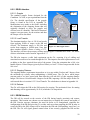
Final Report
Michael Trauttmansdorff (Operations)
Kristian Dixon (Controls)
Stephanie Allen (Electrical)
Mohammad Alam (Systems)
Wassim Abu-Zent (Mechanical)
Rev. ZG
December 6, 2004
I
Acknowledgements
Team HERO would like to thank the following people for their help and support throughout the
design project.
Paul Fulford – MDR Course Coordinator
Tim Reedman
Ross Gillett
Tim Fielding
Perry Newhook
Professor Chris Damaren – U of T Course Coordinator
Luke Stras
Dr. Chad English - Neptec
II
Executive Summary
The Hubble Rescue Mission [2] planned by NASA has a primary objective to safely and reliably
de-orbit the Hubble Space Telescope (HST) and a secondary objective to extend the useful
scientific life of the HST. The mission will be performed by a Hubble Rescue Vehicle (HRV)
which is to consist of a De-Orbit module (DM) which de-orbits the HST, and an Ejection
Module (EM) which supports the Grapple Arm (GA) and Dexterous Arm (GA) and de-orbits
them after the servicing phase is complete.
The following high-level requirements of a robotic servicing mission have been put forth from
NASA Head Quarters:
1. Provide the capability to safely and reliably de-orbit HST at the end of its useful
scientific life
2. Provide the capability to robotically extend the scientific life of HST for a minimum of 5
(TBR) years
3. Provide robotic installation of the WFC3 and COS instruments
4. Provide single-fault tolerance for the de-orbit mission
5. Ensure that Level I performance is not degraded by robotic servicing
As stated in MDR’s request for proposal (RFP) [1], requirements 2, 3, 4, and 5 form the mission
objectives for the Dexterous Robot (DR) system. Additionally, the DR will operate
cooperatively with the Grapple Arm (GA), which provides a platform from which the DR will
perform the servicing tasks.
The design described within this document has the necessary operations policies, systems
architecture, control systems, electrical power supply, and mechanical design to achieve the
above mission, and to satisfy all the necessary requirements.
The DR is able to perform all necessary work within worksites on the HST with an arm span of
4.8 m (2.4 m per arm) and 6 degrees of freedom in each arm. It will be moved from work site to
work site on board the end effector of the GA. A general purpose manipulator arm is used to
handle cables, doors and other fixures on the HST. A tool arm uses interchangeable specialized
tools for tasks such as unscrewing, driving latches, and mating connectors.
The DR will achieve better than required performance through the use of autonomous abilities
such as work site registration and active force control. The DR will compensate for perturbations
during motions which are due to the flexibility of the combined DR/GA structure.
For reliability, the DR has a fully manual backup mode, and has been designed to a maximum
level of redundancy with appropriate factors of safety. HST level 1 performance is preserved by
the hazard mitigation strategy of stopping the GA and DR as soon as fault conditions are
detected, and having ground controllers assess such situations for safety.
Finally, the DR meets all the requirements given by the customer and is the best solution to the
given problem. In short, the DR Rocks!
III
Table of Contents
ACKNOWLEDGEMENTS ......................................................................................................................II
EXECUTIVE SUMMARY ..................................................................................................................... III
TABLE OF CONTENTS .........................................................................................................................IV
1
THIS PAGE INTENTIONALLY LEFT BLANK........................................................................... 1
2
ABBREVIATIONS ............................................................................................................................ 2
3
MISSION OVERVIEW..................................................................................................................... 3
3.1
3.2
3.2.1
3.2.2
3.2.3
3.2.4
3.3
3.4
3.4.1
3.4.2
4
DEXTEROUS ROBOT OVERVIEW .............................................................................................. 6
4.1
4.1.1
4.1.2
4.2
4.2.1
4.2.2
4.3
4.3.1
4.3.2
4.3.3
4.4
5
MISSION SCOPE ...........................................................................................................................................3
MISSION OBJECTIVES ..................................................................................................................................3
Power Augmentation..............................................................................................................................3
Replace aging Rate Sensing Units (RSUs).............................................................................................3
Extend Scientific Life .............................................................................................................................3
Do No Harm to Hubble..........................................................................................................................3
STAKEHOLDERS / USERS .............................................................................................................................3
MISSION PROFILE ........................................................................................................................................4
Mission Phases ......................................................................................................................................4
Mission Systems .....................................................................................................................................4
TOP LEVEL REQUIREMENTS ........................................................................................................................6
Functional Requirements.......................................................................................................................7
Performance Requirements....................................................................................................................7
SYSTEM ARCHITECTURE .............................................................................................................................8
Functional Decomposition.....................................................................................................................8
System Block Diagram.........................................................................................................................10
DR CHARACTERISTICS ..............................................................................................................................11
Physical Architecture...........................................................................................................................11
Power Budget.......................................................................................................................................13
Mass Budget.........................................................................................................................................13
SYSTEM CONCLUSION ...............................................................................................................................13
OPERATIONS ................................................................................................................................. 14
5.1
5.1.1
5.1.2
5.1.3
5.2
5.2.1
5.3
5.3.1
5.3.2
5.3.3
5.3.4
5.4
5.5
5.5.1
5.5.2
5.6
5.6.1
5.6.2
OPERATIONAL OVERVIEW .........................................................................................................................14
Operational Policies ............................................................................................................................14
Operational Constraints ......................................................................................................................14
Operational Environment ....................................................................................................................14
FUNCTIONAL FLOW ...................................................................................................................................15
Operations Timeline ............................................................................................................................15
DR/GA INTERACTION ...............................................................................................................................16
DR grappling and activation ...............................................................................................................16
DR repositioning during servicing.......................................................................................................17
DR / GA emergency stop......................................................................................................................17
DR stow and un-grappling...................................................................................................................17
OPERATING MODES ...................................................................................................................................17
SAFETY .....................................................................................................................................................18
Operational Scenarios .........................................................................................................................18
Failure Modes and Effects Analysis ....................................................................................................19
GROUND CONTROL ARCHITECTURE ..........................................................................................................19
Initiation of Mission Tasks (Internal Interfaces) .................................................................................21
External Interfaces...............................................................................................................................22
IV
5.6.3
Personnel Needs ..................................................................................................................................22
5.6.4
Existing Support Environment .............................................................................................................23
5.7
AUTONOMY ...............................................................................................................................................23
5.7.1
Autonomy Requirements ......................................................................................................................24
5.7.2
Autonomous Architecture ....................................................................................................................25
5.8
OPERATIONS TRADEOFFS ..........................................................................................................................26
6
CONTROL SYSTEM ...................................................................................................................... 28
6.1
6.1.1
6.1.2
6.1.3
6.1.4
6.1.5
6.2
6.2.1
6.2.2
6.2.3
6.3
6.3.1
6.3.2
6.3.3
6.4
6.4.1
6.4.2
6.4.3
6.4.4
6.4.5
6.4.6
6.4.7
7
CONTROL REQUIREMENTS.........................................................................................................................28
Functional............................................................................................................................................28
End Effector Position Accuracy...........................................................................................................28
End Effector Position Resolution.........................................................................................................28
Vision System Sensor Requirements ....................................................................................................28
Time Domain Requirements.................................................................................................................28
CONTROL ARCHITECTURE .........................................................................................................................29
Control Philosophy - Distributed controllers and Centralized Coordination .....................................29
Controlled Devices ..............................................................................................................................29
Controller Overview ............................................................................................................................30
VISION SYSTEM ARCHITECTURE ...............................................................................................................33
Selection of a Primary Vision System Sensor ......................................................................................33
Video Cameras.....................................................................................................................................36
Vision System CPU ..............................................................................................................................36
SOFTWARE ARCHITECTURE .......................................................................................................................37
Software Requirements ........................................................................................................................37
Level 0 - Rationale...............................................................................................................................39
Level 1 Breakdown ..............................................................................................................................41
Level 2 breakdown ...............................................................................................................................45
Example Software Mini-Spec...............................................................................................................48
Data Dictionary ...................................................................................................................................48
Software ‘Push Down’ Hardware Requirements.................................................................................48
ELECTRICAL SUBSYSTEM ........................................................................................................ 49
7.1
ELECTRICAL REQUIREMENTS ....................................................................................................................49
7.2
ELECTRICAL ARCHITECTURE ....................................................................................................................49
7.2.1
External Interfaces...............................................................................................................................49
7.2.2
Cabling Layout ....................................................................................................................................49
7.2.3
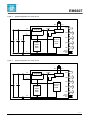
Functional Block Diagrams.................................................................................................................50
7.3
ELECTRICAL SYSTEM IMPLEMENTATION ...................................................................................................52
7.3.1
Power Busses .......................................................................................................................................52
7.3.2
Data Busses .........................................................................................................................................53
7.3.3
Electrical Mass Budget........................................................................................................................53
7.4
FAULT TOLERANCE ...................................................................................................................................53
7.4.1
Automatic Breakers and Fault Recovery .............................................................................................53
7.4.2
Power Bus Redundancy .......................................................................................................................54
7.4.3
Data Bus Redundancy..........................................................................................................................54
7.5
POWER DEMAND .......................................................................................................................................54
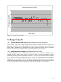
7.6
DESIGN TRADEOFFS ..................................................................................................................................56
7.6.1 Complex Multiple Redundancy vs. Redundancy through Duplication ............................................56
7.6.2 Centralized Device control vs. Distributed Device Control..............................................................56
8
MECHANICAL SUBSYSTEMS .................................................................................................... 57
8.1
MECHANICAL REQUIREMENTS ..................................................................................................................57
8.2
PHYSICAL ARCHITECTURE ........................................................................................................................57
8.2.1
Overview of Mechanical Design..........................................................................................................57
8.2.2
DR/GA Interface ..................................................................................................................................58
8.2.3
DR/EM Interface..................................................................................................................................58
8.3
MECHANICAL SYSTEM IMPLEMENTATION .................................................................................................59
8.3.1
Tool Arm ..............................................................................................................................................59
V
8.3.2
Manipulator Arm .................................................................................................................................61
8.3.3
Body .....................................................................................................................................................62
8.3.4
Tools ....................................................................................................................................................62
8.3.5
Tool Caddy...........................................................................................................................................66
8.3.6
Thermal................................................................................................................................................67
8.4
FAULT TOLERANCE ...................................................................................................................................67
8.5
MASS BUDGET ..........................................................................................................................................68
8.5.1
Cabling and Connector Mass ..............................................................................................................68
8.5.2
Boom Structure/Fairings .....................................................................................................................68
8.5.3
Joint Structure .....................................................................................................................................68
8.5.4
Resolver Mass......................................................................................................................................68
8.5.5
Tool Mass ............................................................................................................................................68
8.5.6
Motor Electronics ................................................................................................................................68
8.5.7
Thermal Protection System..................................................................................................................68
8.5.8
A Final Note.........................................................................................................................................69
8.6
DESIGN TRADEOFFS ..................................................................................................................................69
8.6.1
Joints....................................................................................................................................................69
8.6.2
Booms ..................................................................................................................................................69
9
CONCLUSIONS .............................................................................................................................. 71
9.1
POSSIBLE IMPROVEMENTS .........................................................................................................................71
10
REFERENCES ................................................................................................................................. 72
11
BIBLIOGRAPHY ............................................................................................................................ 73
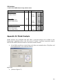
APPENDIX 1
FUNCTIONAL FLOW .............................................................................................. 74
APPENDIX 1.1
FUNCTIONAL FLOW LISTING .......................................................................................................74
Appendix 1.1.1. Launch Phase Functional Flow............................................................................................74
Appendix 1.1.2. Pursuit Phase Functional Flow............................................................................................74
Appendix 1.1.3. Proximity Phase Functional Flow........................................................................................74
Appendix 1.1.4. Capture Phase Functional Flow...........................................................................................74
Appendix 1.1.5. Approach Phase Functional Flow........................................................................................74
Appendix 1.1.6. Jettison Phase Functional Flow ...........................................................................................80
APPENDIX 1.2
CONTINGENCY SCENARIOS .........................................................................................................80
Appendix 1.2.1. Mechanical failure of the 7/16” tool ....................................................................................80
Appendix 1.2.2. Failure of the main power system.........................................................................................81
Appendix 1.2.3. Communications black out due to solar ...............................................................................81
APPENDIX 2
SYSTEM REQUIREMENTS.................................................................................... 83
APPENDIX 3
SYSTEM ARCHITECTURE .................................................................................... 91
APPENDIX 3.1
SYSTEM BLOCK DIAGRAM ..........................................................................................................91
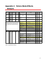
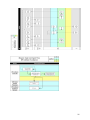
APPENDIX 4
FAILURE MODE EFFECTS ANALYSIS............................................................... 92
APPENDIX 4.1
FREQUENCY AND SEVERITY RATINGS FOR FMEA ......................................................................93
APPENDIX 5
AUTONOMY.............................................................................................................. 94
APPENDIX 5.1
APPENDIX 5.2
LEVELS OF AUTONOMY...............................................................................................................94
COMMAND AND CONTROL FLOW DOWN .....................................................................................94
APPENDIX 6
CONTROLS.............................................................................................................. 103
11.1
11.2
11.3
11.4
11.5
11.6
11.7
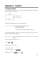
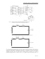
DYNAMIC MODEL ...................................................................................................................................103
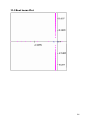
PLANT AND CONTROLLER BLOCK DIAGRAM ...........................................................................................104
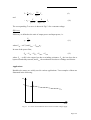
ROOT LOCUS PLOT ..................................................................................................................................106
BODE PLOT..............................................................................................................................................107
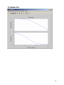
STEP INPUT RESPONSE ............................................................................................................................108
CORRESPONDENCE WITH DR. CHAD ENGLISH PHD. NEPTEC, .................................................................108
DATADICTIONARY ..................................................................................................................................114
VI
11.8
MINI SPECIFICATION FOR MOTOR CONTROL LEVEL 2 ..............................................................................115
APPENDIX 7
ELECTRICAL.......................................................................................................... 119
APPENDIX 7.1
CABLE LAYOUT ........................................................................................................................119
Appendix 7.1.1. Cable Layout Map ..............................................................................................................119
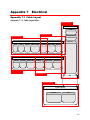
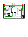
Appendix 7.1.2. Layout and Cabling 1 – Lower Tool Arm...........................................................................120
Appendix 7.1.3. Layout and Cabling 2 – Upper Tool Arm...........................................................................121
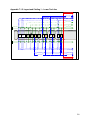
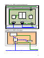
Appendix 7.1.4. Layout and Cabling 3 – Lower Manipulator Arm ..............................................................122
Appendix 7.1.5. Layout and Cabling 4 – Upper Manipulator Arm ..............................................................123
Appendix 7.1.6. Layout and Cabling 5 – DR Body.......................................................................................124
Appendix 7.1.7. Layout and Cabling 6 – EM ...............................................................................................125
APPENDIX 7.2
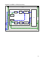
ELECTRICAL FUNCTIONAL BLOCK DIAGRAM............................................................................126
Appendix 7.2.1. High Level EFBD ...............................................................................................................126
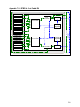
Appendix 7.2.2. EFBD 1 - Motor EU ...........................................................................................................127
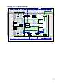
Appendix 7.2.3. EFBD 2 - Thermal Control System.....................................................................................128
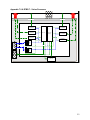
Appendix 7.2.4. EFBD 3 - LCS EU (Control Unit) ......................................................................................129
Appendix 7.2.5. EFBD 4 - Tool Caddy EU ..................................................................................................130
Appendix 7.2.6. EFBD 5 - Tool Gripper MEU.............................................................................................131
Appendix 7.2.7. EFBD 6 - Clamp EU ..........................................................................................................132
Appendix 7.2.8. EFBD 7 - Vision Processor ................................................................................................133
Appendix 7.2.9. EFBD 8 - CPU ...................................................................................................................134
Appendix 7.2.10. EFBD 9 - Force/Torque Sensor Unit ...............................................................................135
Appendix 7.2.11. EFBD 10 - Mini Camera ..................................................................................................135
APPENDIX 7.3
POWER DEMAND .......................................................................................................................136
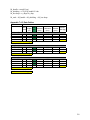
APPENDIX 7.4
DR CABLE MASS ......................................................................................................................137
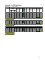
Appendix 7.4.1. Power Cables .....................................................................................................................137
Appendix 7.4.2. Power Sample Calculations ...............................................................................................138
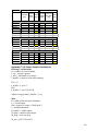
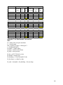
Appendix 7.4.3. Data Cables........................................................................................................................139
Appendix 7.4.4. Data Sample Calculations..................................................................................................140
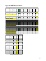
APPENDIX 7.5
GA CABLE MASS ......................................................................................................................141
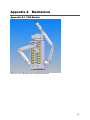
APPENDIX 8
MECHANICAL........................................................................................................ 142
APPENDIX 8.1
CAD MODELS ...........................................................................................................................142
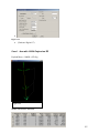
APPENDIX 8.2
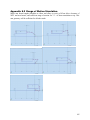
RANGE OF MOTION SIMULATION ..............................................................................................145
APPENDIX 8.3
CALCULATIONS .........................................................................................................................146
Appendix 8.3.1. Tool Manipulator Arm Calculations: .................................................................................146
Appendix 8.3.2. Tool Manipulator Joints Calculations................................................................................147
Appendix 8.3.3. Tool Manipulator Material Selection .................................................................................148
Appendix 8.3.4. General Manipulator Arm Calculations.............................................................................149
Appendix 8.3.5. General Manipulator Joints Calculations ..........................................................................150
Appendix 8.3.6. General Manipulator Material Selection Calculations ......................................................151
Appendix 8.3.7. Motor and Gearbox Calculations.......................................................................................152
Appendix 8.3.8. Motor Sample CalculationsGA Interface ...........................................................................153
Appendix 8.3.8. GA Interface .......................................................................................................................154
APPENDIX 8.4
MODAL ANALYSIS ....................................................................................................................154
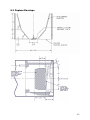
Case 1 - Arm with 1000lb Payload on EE .......................................................................................................155
Case 2 - Arm with no Payload on EE...............................................................................................................156
APPENDIX 8.5
THERMAL CONTROL SUBSYSTEM..............................................................................................158
APPENDIX 8.6
END EFFECTOR PERFORMANCE .................................................................................................161
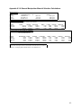
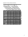
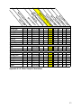
APPENDIX 8.7
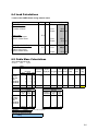
DETAILED MASS BUDGET .........................................................................................................165
APPENDIX 9
DATA SHEETS ........................................................................................................ 167
APPENDIX 10
INTERFACE CONTROL DOCUMENT............................................................... 168
ICD TABLE OF CONTENTS ............................................................................................................... 169
1
ICD NOMENCLATURE............................................................................................................... 170
2
ICD MECHANICAL INTERFACE............................................................................................. 171
VII
2.1
2.2
2.3
2.4
2.5
STRUCTURE .............................................................................................................................................171
DR STOW CONFIGURATION .....................................................................................................................171
CAPTURE ENVELOPE ...............................................................................................................................172
LOADING .................................................................................................................................................172
THERMAL ................................................................................................................................................172
3
ICD ELECTRICAL INTERFACE............................................................................................... 173
4
ICD SOFTWARE INTERFACE .................................................................................................. 174
4.1
COORDINATE SYSTEMS ...........................................................................................................................174
4.2
COMMUNICATIONS ..................................................................................................................................174
4.2.1
Emergency Stop Command ................................................................................................................174
4.2.2
From Ground Control to DR/GA.......................................................................................................174
4.2.3
From DR/GA To Ground Control......................................................................................................174
4.2.4
DR Ground Control to GA Ground Control ......................................................................................175
4.2.5
GA Ground Control to DR Ground Control ......................................................................................175
5
ICD REFERENCES....................................................................................................................... 176
6
ICD APPENDICES ........................................................................................................................ 177
6.1
6.1.1
6.1.2
6.1.3
6.2
6.3
6.4
6.5
6.6
6.6.1
6.6.2
GA END EFFECTOR .................................................................................................................................177
Front View .........................................................................................................................................177
Isometric View ...................................................................................................................................178
Interface Teeth Detail ........................................................................................................................179
DR STOW CONFIGURATION .....................................................................................................................180
CAPTURE ENVELOPE ...............................................................................................................................183
LOAD CALCULATIONS .............................................................................................................................184
CABLE MASS CALCULATIONS .................................................................................................................184
ELECTRICAL INTERFACE REQUIREMENTS ................................................................................................185
Power Interface .................................................................................................................................185
Data Interface....................................................................................................................................185
APPENDIX 11
CLASS PHOTO........................................................................................................ 187
VIII
1 This page intentionally left blank
1
2 Abbreviations
Abbreviation
Definition
AFC
C&DH
CU
DR
DM
DOF
EE
EL
EM
EMI
EPS
EU
FMEA
FRGF
FTSU
GA
GC
HRM
HRV
HST
ICD
IR
IRED
LCS
MEU
MH
PWM
RFP
RSS
RSU
SP
SR
TBD
TBR
TCS
WFC3
WF/PC2
WP
WR
WRT
WY
Active Force Control
Command and Data Handling
Control Unit
Dexterous Robot
De-Orbit Module
Degrees Of Freedom
End Effector
Elbow
Ejection Module
Electro Magnetic Interference
Electrical Power System
Electrical Unit
Failure Mode Effects Analysis
Flight Releasable Grapple Fixture
Force Torque Sensing Unit
Grapple Arm
Ground Control
Hubble Rescue Mission
Hubble Rescue Vehicle
Hubble Space Telescope
Interface Control Document
Infra Red
Infra Red Emitting Diodes
Laser Camera System
Motor Electrical Unit
Manipulator Hand
Pulse Width Modulation
Request For Proposal
Robotic Servicing System
Rate Sensing Unit
Shoulder Pitch
Shoulder Roll
To Be Determined
To Be Reviewed
Thermal Control System
Wide Field Camera 3
Wide Field / Planetary Camera 2
Wrist Pitch
Wrist Roll
With Respect To
Wrist Yaw
2
3 Mission Overview
3.1 Mission Scope
The scope of the DR mission is limited to the robotic servicing portions of the Hubble Rescue
Mission (HRM) as presented by the contractor, MD Robotics, in the Request For Proposal (RFP)
[1]. It will consist of the robotic mechanisms and support systems required to perform the power
augmentation, wide field camera change out, and gyroscope installation operations during the
servicing phase of the mission.
The DR shall operate in concert with another robot, the Grapple Arm, which will serve as a
mobile platform from which the DR will operate. Power and communications will be provided to
the DR from the systems in place on board the EM component of the HRV, and the DR will be
stowed on the EM when not in use.
3.2 Mission Objectives
3.2.1 Power Augmentation
The DR is responsible for connecting the power conduits to the +V2 and –V2 diode boxes. This
conduit connects the HST solar panels to the new batteries on board the de-orbit module.
3.2.2 Replace aging Rate Sensing Units (RSUs)
The DR is responsible for installing new Rate Sensing Units (RSUs) to allow the HST to
maintain pointing control when one of the remaining three RSUs fails. This will be accomplished
by installing the Wide Field Camera 3 (WFC3) on which the new RSUs are mounted.
3.2.3 Extend Scientific Life
The repair of HST power and pointing systems will extend the scientifically useful life of the
HST for a number of years. Additionally, the WFC3 will expand the capabilities of the HST,
further increasing the scientific value and potential of the Hubble Mission.
3.2.4 Do No Harm to Hubble
During all parts of the mission, Level 1 performance of the HST must not be degraded. The DR
will operate so as to do no harm to the HST.
3.3 Stakeholders / Users
The main user of the DR system is the NASA HST mission team. This team requires a reliable
and effective robotic servicing system to fulfill their mission objectives. The operators of the DR
will be specially trained NASA mission personnel responsible for directing the DR in the
servicing operations.
Indirect stakeholders in the DR are the members of the scientific community who will benefit
from the extended life and enhanced scientific capabilities of the HST. Also, the space robotics
industry stands to benefit from the technologies developed for this mission, and from the
experience gained in performing orbital robotic servicing.
3
3.4 Mission Profile
3.4.1 Mission Phases
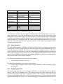
The role of the DR in context of the Hubble Rescue Mission’s phases is described in Table 3.1.
The scope of DR primary operations is within the servicing phase of the mission. The DR acts as
a payload on board the EM during the remainder of the mission.
Phase
Duration
DR Operations
Purpose
Launch
Pursuit
Proximity
Operations
Capture
Servicing
2 hours
2-12 days
1-2 days
Off
Off
Off
Payload
Payload
Payload
2 hours
30 days
Off
Activation
Service Ops
EM Jettison &
Disposal
Science Operations
De-orbit
4 days
Shutdown
Payload
Augment EPS
Install RSUs
Install WFC3
End of Life
(Payload)
5 years +
4 days
None
None
Table 3.1 – Mission Phases and Systems
3.4.2 Mission Systems
The major systems involved in the execution of the Hubble Rescue mission, other than the
Dexterous Robot, are as follows:
3.4.2.1 Hubble Rescue Vehicle (HRV)
This spacecraft is made of two components, the De-Orbit module (DM) and Ejection Module
(EM). The HRV will transfer from its initial low earth orbit to perform a rendezvous with the
HST, allowing the robotic systems to perform the capture and servicing operations.
3.4.2.2 De-Orbit Module
This spacecraft will carry out the primary objective of the HRM, namely the controlled de-orbit
of the HST. However, prior to this terminal phase of the mission, it will serve as the structural
attachment between the HST and the EM (and thus the RSS). It also contains the auxiliary
batteries that will extend the functional life of the HST.
3.4.2.3 Ejection Module
This spacecraft contains the GA and DR robots, as well as the electrical power systems (EPS),
communications hardware, and new HST components. During launch, pursuit, proximity,
capture, and de-orbit the DR is stowed as a payload on the side of this module. At the end of the
servicing mission this module separates from the HST-DM unit, and is de-orbited along with the
on board GA and DR.
4
3.4.2.4 Grapple Arm
This robot performs the mission critical capture operation, and brings the HRV into alignment
for docking with the HST. Additionally, it serves as the primary platform from which the DR
operates during the servicing phase. The GA positions the DR at the necessary work sites,
provides a structural support, and is a conduit for the DR’s electronics and data cables
connecting it to the Ejection Module.
5
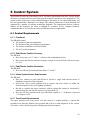
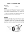
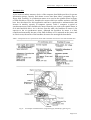
4 Dexterous Robot Overview
The purpose of the Dexterous Robot (DR) is to
perform three main tasks. It must perform power
augmentation operation, replace the old WF/PC2
camera with the new WFC3 camera and replace the
RSU’s in the process. We look at the DR from a
systems point of view in this section. The basic
functional and performance requirements were
provided in the RFP [1] and these were broken
down to give detailed functional and performance
requirements.
Vision Sys
Manipulator
Arm
Tool Arm
The DR has the following major systems:
1) Vision
The vision system is comprised of the LCS
Tool Caddy
(3D laser scanner), four mini cameras and
IR sensors enabling the operators and the
DR to be aware of the environment.
Figure 4.1 - DR Overview
2) Two manipulator arms
Each arm has a span of 2.4 m with six
degrees of freedom and a tip resolution of 0.025mm (translation) and 0.011 degrees
(rotation), giving the DR the ability reach and access all parts of the workspace.
3) Communication
The communication system enables the DR to constantly update ground control about the
workspace situation and receive new commands and scripts.
4) Survival
The survival system enables the DR to keep alive and maintain its system. This includes
the thermal control and the fault monitoring and control system.
5) Control
The control system controls the process and actions carried out by the DR to complete the
mission.
6) Tools
The tools enable the DR to interface with the HST in order to perform its mission.
These seven systems enable the DR to satisfy all given customer requirements.
In the following sections we present the customer requirements, system architecture, system
block diagram showing the top level components of our system, physical architecture and the
summarized power and mass budgets.
4.1 Top Level Requirements
The top level requirements were derived from the RFP and these were broken down further to
get the system requirements on which our DR design was derived. The sections that follow
present these requirements and the top level system architecture designed to satisfy these
requirements followed by a system block diagram that outlines these systems.
6
4.1.1 Functional Requirements
The DR shall be able to perform the following operations:
DR.F1 Power augmentation
DR.F1.1 Tap SA3 power at P6A and P8A on both HST diode boxes.
DR.F1.2 Rout SA3 power to DM via new harness
DR.F1.3 Harness Attachments (12 locations) to hold down conduit
DR.2 WFC3 installation
DR.F2.1 Attach new ground strap stowage fixture
DR.F2.2 WF/PC2 Interface plate
DR.F2.3 WF/PC 2 blind mate release
DR.F2.4 Release and secure Ground strap
DR.F2.5 Release A latch
DR.F2.6 Remove and stow WF/PC2
DR.F2.7 Retrieve and position WFC3
DR.F2.8 Install WFC3 into telescope
DR.F2.9 Replace latch A
DR.F2.10 Replace ground strap
DR.F2.11 Replace blind mate
DR.F2.12Final stow WF/PC2
DR.F3 Gyro data and power augmentation
DR.F3.1 486 - 1553 data bus installation (J9 connector on HST bay 1)
DR.F3.2 Power for Gyros supplied by harness from DM to WFC3
DR.F4 All the above functions have to be performed while being supported by the GA and
therefore have to satisfy interface requirements from the GA team
4.1.2 Performance Requirements
The DR shall:
DR.P1 Capable of maneuvering arm/s anywhere in the workspace
accuracy of ± 1° relative to commanded position
resolution better than 0.1” and 0.1°
DR.P2 Torque drive of 50 ft-lb and
DR.5.1 track the progression of tool by counting turns and monitoring torque
DR.P3 Be capable of stopping a 1000lb mass from maximum commanded tip velocity within 2”
and 2°
DR.P4 DR shall be capable of limiting forced normal to constrained translational paths to no
more than 10lbs and delivering up to 25lbs along those paths
DR.P4.1 Shall have a six axis force and torque sensor near end effector to sense the
torque and force at end effector with accuracy of less than ±2lbs and ±2ft-lb as
measured at end effector
DR.P5 Consume less than 300W that has been assumed to be the current power budget.
DR.P6 Weigh less that 500Kg which we assumed is the mass budget allowed.
The detailed requirement tree derived from these requirements can be found in Appendix 2
7
4.2 System Architecture
4.2.1 Functional Decomposition
The following are the basic functions that the system needs in order to complete the mission.
Vision system
The DR will be equipped with two camera systems that include one laser camera system (LCS)
and four mini cameras.
The LCS by Neptec provides xyz workspace data. The LCS has a range of 30m and an accuracy
of ±2mm within a 5m range. See Table 6.1 for details. Two mini cameras will be located at each
end effector. These will be used to provide video feedback to GC.
System Interfaces
To perform the required operations the DR has to interface with the surrounding systems
including HRV, HST, GA, and GC. The most important interface for the mission is the interface
between the GA and DR. This interface is basically a modification of the FRGF. The details of
the ICD can be found in Appendix 10.
Communication System
The communication system has three parts:
1) Communication within DR
The various parts of the DR have to be able to communicate with each other and the
CPU. Most of the components of the DR are connected to the central computer via a
MIL –1553 data bus. The LCS requires a high data transfer rate and high processing
power. Thus it will have a separate CPU and will be connected to the vision system
CPU using a separate MIL – 1553 data bus. The vision system CPU and the main
CPU will be in communication with each other in the avionics box.
2) Communication with GA
The DR CPU and the GA CPU will be in communication to notify each other of new
coordinates and emergency halt commands.
3) Communication with GC
The communication with GC will be achieved using the EM communication module.
This is necessary to keep GC aware of the current situation and to receive and new
scripts and commands from GC.
Survival system
The purpose of our survival system is to ensure that the DR is not damaged or rendered
inoperable during launch or operational phase. This system includes thermal control and fault
monitoring.
The heating system uses thermocouples located at thermally sensitive locations to determine
whether active heating is necessary. Unless active heating is necessary the temperature is
maintained using passive heating and cooling. The heating element will be Kapton heaters (see
Appendix 8.5) and to prevent over cooling MLI insulation blankets will be used. Since the DR
has to be single fault tolerant most vulnerable systems are duplicated and the survival system
will detect failure to any of these components and switch to the backup. Such systems include
the electrical cabling, data bus, lights, mini cams, motor winding and others.
8
Other sensing capabilities
We decided to provide the DR with two other sensing capabilities that are
1) IR sensors: The IR sensors are located in specific locations on the DR that are not in
the field of view of the LCS or the mini cams. The purpose is to detect if those parts
are too close to the Hubble.
2) We will also use touch/pressure sensor in the tool caddy to register whether the tools
are in position. When the tool arm acquires the tool it applies a pressure that
stimulates the release of the right tool.
Control system
The control system of the DR is comprised of the various sensors that report telemetry to the
C&DH where software processes this data and produces output signals to actuators/devices that
creates the necessary response. The major part of the control software is the control of the
motors. According to the calculated response time and due to the fact that we decided that
absolutely no overshoot is acceptable we decided use a second order control transfer function
with simple P control with data from the resolvers forming the feed back loop.
Central C&DH
The central CPU will be located in the avionics box in the EM. Since the vision data processing
requires large processing powers we decided to have a separate CPU to perform model matching
and analyzing the data from the LCS and the four Mini Cameras.
9
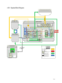
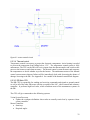
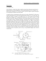
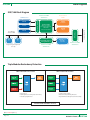
4.2.2 System Block Diagram
Hubble Space Telescope
Tools
Used
To
Perform
Service
Functions
Grapple Arm
Dexterous Robot
WF2/C
Temporary
Stow
Fixture
`
GA
Grappling
DR
Thermal Control System
End Effector
Mechanism TCS
Backup
Power
Bus
Primary
Power
Bus
7/16" Tool
Sensors
Joint
Joint
Joint
Mechanisms
Mechanisms
Mechanisms
Structural
Mechanisms
`
Sensor Relay
Temp
Sensor
Joint Relay
Grapple Fixture
Sensor Pointing
Mechanism
Angle Sensor /
Encoder
Angle
Sensor
GA
EPS
6 D.O.F. Force/
Torque Sensor
End Effector
Relay
Angle Sensor /
Encoder
Actuators
Temp
Sensor
Backup
Data
Bus
Temp
Sensor
GA Data
Connection
DR C&DH
System
Safety Fuses
Primary
Data
Bus
Ground Control
Operators & Customer
Radiative Heat Loss
Temp
Sensor
Docking Latches
and Hardpoints
Temp
Sensor
C&DH TCS
`
Solar Heat
Tool Gripping /
Drive
Mechanism
Temp
Sensor
EPS TCS
GA Power
Connection
End Effector
Mechanism
Force/Torque
Sensor
Sensor Pointer
Relay
Safety Fuses
General
Purpose
Clip
Sensor System
Joint TCS
Ejection Module
DBA
Connector
Tool
Tools
Camera TCS
Camera Positioning
Mechanism TCS
RSU
Conenctor
Tool
LEGEND
Satellite Data
Link
Greyed Out Box
Blocks External to, but interfacing
with, the RSS
Black Bordered
Box
Blocks Representing Subsystems
of the RSS
Grey Filled Box
Blocks Representing Subsystem
Components
Mechanical Interface
Thermal Interface
`
Ground Control Station
User Interface
Ground Control
Station User
Interface
Large
Arrows
Ground Control
Comm
System
External / Environmental
Interfaces to the RSS
Medium
Arrows
Internal Interfaces between
Subsystems of the RSS
Small Arrows
Internal Interfaces between
Subsystem Components
Sensory / Data
Interface
Electrical Interface
10
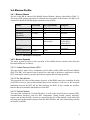
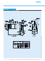
4.3 DR Characteristics
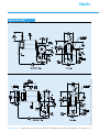
4.3.1 Physical Architecture
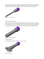
Figure 4.2 Front view of DR
11
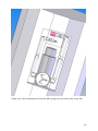
Figure 4.3 Rear View of the DR
12
This section summarizes the physical architecture of the DR. and briefly describes the five major
physical structures, the main body, tool arm, gripper arm, head (housing the LCS) and grapple
fixture. Figure 4.2 shows the front view of the DR. Here the six joints of both arms are visible
along with the tool caddy and the LCS mounted on the head. We can also see the various
stowage fixtures. Figure 4.3 shows the rear view of the grapple fixture with the two target
points, two power connectors and two data connectors.
The body houses the tool caddy the two shoulder roll motor and the power and data busses going
to the arms and the LCS. The length of the body is 140 cm and has a diameter of ∼ 58cm.
The arms have a total span of ∼2.4m. They have 3 main segments shoulder, arm booms, wrist
and end effectors. The arm booms each have a length of 85 cm. The shoulder and wrist roll
motors have a range ±180°, the shoulder pitch, the elbow and the wrist pitch and yaw motors
each have a range of ±135° giving the DR the range of motion necessary to complete the
mission.
The LCS, mounted on the head, is controlled by two motors, enabling it to pan ± 90° and tilt
±45°. This ability gives the LCS a large field of view, which is highly beneficial for the mission.
The grapple fixture is a modified version of the FRGF. The chief modifications being two
targeting points, two data bus connectors, two power bus connectors and 24 gripping teeth. The
purpose of the gripping teeth is to prevent rotational motion while mated to the GA.
The DR has two specialized end effectors; one for handling tools and payloads and the second is
a general purpose gripper to hold loose objects stabilize payload and assist vision system with its
two cameras.
4.3.2 Power Budget
The total average power needed for the DR servicing mission is 145 W.
4.3.3 Mass Budget
The total mass of the DR is 340 kg.
4.4 System Conclusion
The HRV mission presents several engineering challenges. On-orbit robotic servicing will
require significant improvements in control, communications, imaging systems and machine
vision. While NASA has requested that the HRV not be an R&D project, it is apparent that some
new technologies like the LCS are needed in order to carry out the mission. We had to consider
technologies that have not been verified for use in space. This is especially important given that
NASA needs to have the HRV in a timely fashion and in a form that it is reliable enough to
service the one of the most valuable space assets in orbit.
13
5 Operations
This section describes the operations and procedures followed by the DR and its controllers in
carrying out the mission tasks identified in section 3 (above). Hazard mitigation and system
autonomy are also discussed.
5.1 Operational Overview
5.1.1 Operational Policies
In order to maximize the likelihood of the success of the primary and secondary mission
objectives, the DR is required to have limited single fault tolerance. We designed the functional
flow of the mission to accommodate appropriate fail-safes, redundancies, and contingency
scenarios.
It is paramount that the DR does not degrade the Level 1 performance of Hubble during
servicing operations. Appropriate control precision, reliability, safe-modes and abort scenarios
were therefore designed. Additionally, we designed the DR to prevent orbital debris production,
so as not to create a hazardous debris cloud around the HST.
5.1.2 Operational Constraints
The DR operates on power supplied from the EM’s on board Electrical Power System (EPS).
The DR shall interface with communications systems found on the EM for data communication
with Ground Control. It is assumed that the EM communication system will be sufficiently
reliable and have sufficient bandwidth to allow operation of the DR during all mission phases.
The configuration of the HST is fixed, and therefore all operations are designed to be performed
successfully within the envelopes defined by the HST work sites.
Due to the performance demands of the mission, and the lag in radio communications to LEO,
the DR is capable of performing simple scripted tasks such as tip motions or tool actuation in an
autonomous fashion. These scripted tasks will always be initiated by ground control.
The mission must be completed prior to the expected failure date of one of the remaining three
RSUs so as to prevent the HST from entering an uncontrolled and unrecoverable spin. This puts
the servicing phase of the mission no later than mid 2009.
5.1.3 Operational Environment
When launching the HRV, thrusts from the rockets will pulsate and cause the rocket and HRV to
vibrate. The HRV must withstand these vibrations and reach HST unharmed.
HST is a Low Earth Orbiting (LEO) satellite; its orbit is in the thermosphere (HST is at an
altitude of approx. 600km) [3]. The pressure at this altitude is very low (almost zero) and
temperature gradients during each HST orbit can vary over 100°F as the Earth blocks out the
sun’s light. Temperatures range at this altitude from 300°F to –300°F. The DR has been
designed to regulate its temperature to ranges that are survivable by its subsystems (see appendix
8.5).
14
The mission needs to be carried out without blocking Hubble’s solar arrays, communication
receivers/transmitters or the Tracking and Data Relay Satellite System (TDRSS).
At Hubble’s altitude, the overhead atmosphere (the exosphere) does not provide any significant
radiation protection. We have therefore designed the systems of the HRV to withstand this harsh
radiation environment.
5.2 Functional Flow
The operational process is described in detail in Appendix 1. The HRV is to be first packaged
securely on the rocket launcher so that it survives the launch loads and vibrations. After launch,
the rocket separates and the HRV will pursue the HST using its guidance/navigation systems.
The DR remains in a keep-alive mode until the GA has captured the HST and docked the HRV
on its berthing pins.
The GA will then mate to the DR, allowing it to power up and detach from the EM. The GA will
then position the DR as required to perform servicing operations that include power
augmentation, installation of the new Wide Field Camera 3 and RSU connections. During
servicing, the DR will have to ensure that all loose parts are stowed properly and not set adrift in
open space. At the completion of servicing task, all tools and components removed from the
HST will be properly stowed on the EM.
After servicing is complete, the GA will stow the DR back onto the EM, placing it within its
stow fixtures and releasing the grapple fixture once the DR has powered down. Once GA has
stowed itself, the EM will jettison from the HST/DM and will be de-orbited. The De-Orbit
module will remain attached to the Hubble for future controlled de-orbit of the HST/DM
complex.
5.2.1 Operations Timeline
This section describes the basic timeline of DR operations. We decomposed the Functional Flow
Block Diagrams from the mission objectives, and detailed them sufficiently to allow the
identification of all significant functional requirements imposed on the DR by its mission.
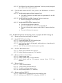
Listed below are the top levels of functional flow during the major parts of the DR mission. A
more detailed functional flow of the DR system is presented in the detailed Functional Flow in
Appendix 1.
1. Launch
1.1. Pre-launch system check
1.2. DR enter keep-alive mode
5. Servicing
5.1. Deploy DR
5.1.1. Activate GA
5.1.2. Move to DR stow site
5.1.4. Grapple DR
5.1.5. DR Wake up & Checkout
5.1.6. DR standby
15
5.1.6.1 DR switches from Normal to Sleep Mode
5.1.6.2 Await command signal from ground control
5.2. Power Augmentation
5.2.1. Conduit Deploy
5.2.2. Diode Box -V2
5.2.3. Diode Box +V2
5.3. WFC3 Operations
5.3.1. Remove Ground Strap
5.3.2. Remove and Temporarily Stow WF/PC2
5.3.3. WFC3 installation
5.3.4. Permanently Stow WF/PC2
5.3.5. WFC3 Support Hardware
6. EM Jettison and De-Orbit
6.1. DR shutdown
6.1.1. Activate GA
6.1.2. Activate DR
6.1.3. Move GA/DR to DR stow site on EM
6.1.5. Configure DR for stowage
6.1.6. GA Positions DR in large capture envelope of main stow fixture
6.1.7. GC engages main stow fixture, aligning DR with other fixtures.
6.1.8. GA tilts DR to position it within capture envelope of remaining
stow fixtures
6.1.9. GC engages remaining stow fixtures as required
6.1.10. DR shuts off power completely
6.1.11. GA releases DR
6.1.12. GA standby
6.2. GA shutdown
6.3 EM Jettisons and Carries out De-Orbit maneuver
Upon the completion of primary and secondary mission objectives the Ejection Module carrying
the RSS will be disposed via separation and subsequent de-orbit. The HST will continue to
produce useful scientific data for an expected period of 5+ years after the end of the DR mission.
5.3 DR/GA Interaction
This section describes the coordination of the DR and GA
operations and explains how the two robots interact. The
DR and GA will interact in four major ways during the
mission:
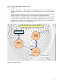
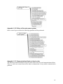
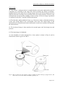
5.3.1 DR grappling and activation
The DR will be in keep-alive mode until the capture phase
of the mission is complete. Once the GA is ready, it will
move to the DR stow site on the side of the EM, and
position itself to grapple the exposed DR Grapple Fixture
(GF). To simplify the operation, we designed the GF on the
DR to emulate a standard FRGF like those on the HST and
positioned it so that it is exposed and easy to reach.
Figure 5.1 - DR is stowed face down
with GF exposed for easy access.
16
The DR will be a passive target during this phase, as its primary systems will be un-powered
until the GA has made the power and data connection. DR ground control will await
confirmation of successful structural and connector mating, and will then activate the main
power and data systems of the DR. This will supply power to the robotic part of the DR via
busses running along the GA. Once the DR has been activated and tested, the stow fixtures will
release, and the GA will move the DR clear of the EM for final testing.
5.3.2 DR repositioning during servicing
During servicing operations the DR will need to be moved from work site to work site by the
GA. The DR has an arm span of about 4.8 m (2.4 meter arms), so it is capable of reaching all
necessary parts of a given work site while executing servicing tasks. However, the servicing
operations take place at various sites, necessitating DR mobility.
Combined motion will be accomplished by the series of operations described in the second
‘Combined GA/DR Move’ Command and Control Flow Down
EM
diagram in Appendix 2. In essence, the DR will assume a static
configuration, the GA will move to the new location, and then the DR
will resume operations
5.3.3 DR / GA emergency stop
In the event of a contingency situation arising, we have identified a
full stop of activities as being the best hazard mitigation strategy (See
5.5 – Safety below) . For this reason, the DA and GR will coordinate
emergency stops so that both systems halt completely in the event of
some fault being detected.
5.3.4 DR stow and un-grappling
The DR needs to be re-stowed prior to jettisoning of the EM. We have
designed the stowing operation to account for the accuracy capabilities
of the GA (See ICD in appendix 10) by making the first stow fixture GA
have a large capture envelope. The DR will be configured for stowing,
and the GA will then need to place the matching fixture on the DR into
the initial stow fixture.
DR GC will then engage this initial fixture to force the DR into
alignment with the remaining connection points. The GA will then
pivot the DR around the closed stow fixture until the remaining ones
are aligned and can be engaged. Once the DR is secure, it will shut
down all systems in anticipation of power being severed one the GA
un-grapples and moves into its own stow position.
Figure 5-1 DR ready
configuration
for
placement in stow
fixtures on EM
5.4 Operating Modes
5.4.1.1 Keep-alive Mode
In this mode the DR be essentially inactive. All CPUs, motors and vision systems will be shut
down to conserve power, aside from the minimum necessary to run the Thermal Control System
17
(TCS). This mode will be used during the launch, pursuit, proximity, and capture phases while
the DR is a payload on the EM.
5.4.1.2 Standby Mode
In this mode the DR will monitor its temperature and power heaters as needed to maintain its
minimum temperature. All processors are on, and the DR is essentially just awaiting the next
command from ground control.
5.4.1.3 Normal mode
In this mode the DR will perform its servicing operations making use of its full set of on board
autonomous capabilities. Arm motions and forces will be autonomously corrected as outlined in
section 5.5 below.
5.4.1.4 Manual mode
In this mode operators will be able to control some, or all, subsystems on the DR directly in the
event of primary control systems failure or if some contingency operation calls for it.
5.4.1.5 Safe Mode
In the event of a fault being detected on the DR, it shall cease all motion to ensure no harm
comes to the HST, send a notification signal to the GA and to GC. The DR will then send
telemetry to GC and await instructions. In the event of a stop during some major operation,
ground controllers will need to decide an appropriate course of action sufficiently quickly to
prevent damage such as having the system freeze to death.
5.5 Safety
5.5.1 Operational Scenarios
Many different operating scenarios may take place during the mission. The nominal operations
scenario is outlined in detail in 1.Appendix 2. In case of failure, the general operating scenario is
defined as follows:
1.
2.
3.
4.
5.
6.
7.
8.
9.
DR automatically enters safe mode
DR resets systems
DR performs safety and operational self tests
If problem successfully eliminated then return to nominal operations
If unsuccessful, DR awaits further instructions from GC
GC identifies solution
Solution is implemented
DR performs safety and operational self tests
Nominal operations resume
The operations procedures used to mitigate a set of specific failures characteristic of the potential
operational disruptions are discussed in Appendix 1.2
Mechanical failure of the 7/16” tool – Appendix 1.2.1
Failure of the main power system – Appendix 1.2.2
Communications black out due to solar interruptions – Appendix 1.2.3
18
5.5.2 Failure Modes and Effects Analysis
In response to the mission requirement that the DR do no harm to the Hubble Space Telescope,
we performed Failure Modes and Effects Analysis (FMEA) on the operations performed by the
DR. The table shown in Appendix 4 illustrates this analysis as broken down into the following
steps:
5.5.2.1 Hazard Identification
First, we identified the various categories of maneuvers performed by the DR. For each of these
actions, a frequency index was assigned based on the scale given in Appendix 4.1. We then
identified the key input and how damage will be caused to the HST. Following this, the failure
modes and effects were listed. The severity of all potential DR failure effects was very high due
to the importance of not harming the HST. See Appendix 4 for the severity index scale.
5.5.2.2 Hazard Mitigation
The second part of the FMEA involved outlining strategies for controlling each hazard. The
potential causes of the failures were outlined, completing the identification and organization task.
We first considered ways to eliminate the hazards from the mission entirely. If this was not
possible, design features were identified that could remove or control the hazard. Finally, in
some instances neither of these options was possible, so we considered methods of reducing the
damage caused by the hazard. See Appendix 4.1 for the control index.
We then assigned a risk index to each series of control actions based on the three categories
discussed above. This allowed for easy identification of the most serious risks to the mission.
All but one of these high-risk failures fall into the group of communication failures during
operations of the DR. These pose the highest risk to the mission because short of having an
entirely redundant communication system, the possibility of failure cannot be eliminated.
Furthermore, the frequency of these actions is very high, increasing the likelihood of a failure
during their operations. Therefore our overall hazard control strategy is to have the DR cease all
motion and await further instructions from ground control.
The last high risk factor falls into the group of command corruption, and we have decided to
mitigate this by having all mission commands and signals use a double-positive system. This
way no single failed channel, or misinterpreted signal, can lead to uncommanded control input to
the DR.
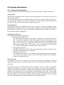
5.6 Ground Control Architecture
This section defines the ground control architecture that will govern how operators carry out the
Dexterous Robot’s repair mission. DR ground control is responsible for all mission tasks, while
the DR subsystems will govern low-level operations that maintain basic functions like thermal
control.
We have reducing the DR to a minimum level of autonomy, as this preserves the same overall
mission capabilities while eliminating failure points, including a number of catastrophic
scenarios (i.e.- a runaway robot completing servicing tasks incorrectly and causing damage to the
HST).
19
The onboard systems of the DR will not be truly autonomous, though they will provide real time
corrections and adjustments while executing the commands issued by ground controllers. Details
of the DR’s autonomy are discussed in section 5.4 (below). The following is a discussion of how
the human controllers of the DR command and control the robotic system during its various
activities.
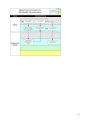
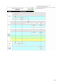
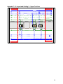
Below is a table identifying what the mission tasks initiated by GC, and those performed by on
board systems without an operator in the loop.
Mission Tasks
Operational Command Tasks
Grapple DR
Deploy DR
DR Self Test
Performance Asessment
Manual operations (I.e. drive a motor)
Service Operation
Grapple tool
Move DR EE to target location
Have GA move DR to a new Work Site
Stow DR
GC Communication Tasks
Establish Communications
Video/LCS downlink
Telemetry Transmission
Update DR software
Low-level continuous tasks
DR Keepalive
Initialize/Refresh Workspace Registration
Collision/Fault Detection
Emergency Stop Signal
Mechanical Sensors (resolvers)
Thermal Control
Ground Control
(Manual)
DR
(Automated)
x
x
x
x
x
x
x
x
x
x
x
x
x
x
x
x
x
x
x
Table 1 – Mission Task Initiators
20
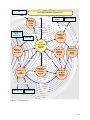
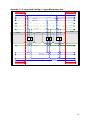
Below is a diagram outlining the subsystems that play a role in the command flow within the DR
system. It also places them in context with external systems that have command interactions with
the DR during its mission.
Colission Detection
System
Emergency Stop
Thermal
Controllers
Main CPU
Motor
Controller(s)
LCS
System
Grapple Arm
Vision System CPU
Communications Link (via Ejection Module)
NASA
Mission
Controllers
and Personnel
Video
Camera
System
Communications Link
DR Ground Control
Communications
Link
Communications
Link
GA Ground Control
Figure 5-2 - Ground Control Architecture (Solid arrows indicate commands
from GC. Dashed Arrows indicate autonomously command signals initiated by
the DR. Thick solid arrows indicate external interfaces with GC. Grey blocks are
systems and actors external to the DR.)
5.6.1 Initiation of Mission Tasks (Internal Interfaces)
DR operations such as servicing tasks will be orchestrated by ground control sending
combinations of available command types to the DR. This methodology can be likened to giving
the DR a script to follow, and telling it when to carry out a particular line. By tailoring the
scripts, which the DR executes on orbit, ground controllers maintain control of the robot at all
times but still benefit from its real-time control capabilities that it uses while executing a
particular given script. Typical commands are an EE move, where ground controllers could
specify a destination point, or a constrained path along which the EE should travel.
For example, to remove a bolt, ground controllers would first initiate a combined move of the
GA/DR. Then they would have the DR acquire the correct tool. Next they would command the
DR to position the tool on the bolt, an operation that would make use of the DR’s greatest on
board autonomous capabilities. While moving the tool from its original location to its final
position on top of the targeted bolt the DR will use its vision system to provide registration
(calibration of the tool position relative to the target location) and correct for any perturbations in
21
its position. Next ground controllers would command the DR to drive its wrist motor to turn the
bolt the desired number of times.
Ground control would upload a part of the above instruction set to the Main CPU on the DR,
which would then execute the instructions by coordinating subsystems on board the DR. In this
manner, by stitching together the various commands that are used to trigger mission tasks on
board the DR, ground controllers will ensure that the mission objectives will be met.
In the event of CPU failure, ground controllers have the capability to command joint motors and
other subsystems directly in manual control mode. This mode provides extra reliability, but does
not offer the same level of performance since the real-time autonomous functions performed by
the CPU are unavailable.
5.6.2 External Interfaces
Ground control needs to interact with NASA mission controllers and operators while performing
servicing tasks on the HST. In the likely event that operations need to be modified or updated
due to unforeseen complications during the mission, DR GC will collaborate with HST
specialists and operators to lay out the functional flow and objectives of any necessary
operations.
Ground control also needs to interact with GA Ground control to coordinate the operations of the
two robotic elements of the RSS. The following information will regularly be exchanged
between DR and GA ground controllers during the operational life of the DR:
DR GC To GA GC:
• Readiness to grapple, prior to un-stowing.
• Readiness to be moved away from open stow fixtures.
• Desired position and orientation to which the GA should move the DR
• Envelope and mass of the DR and any payload prior being moved.
• Resolution of Emergency Stop condition
• Readiness to be placed in open stow fixtures.
• Readiness to un-grapple after stowing. (Ready to power off)
From GA GC:
• Successful grapple of DR.
• Successful mating of connectors on DR GF. (Ready to power on)
• Resolution of Emergency Stop condition
• Arrival at requested location.
• Successful un-grapple and de-mating of connectors on DR GF.
5.6.3 Personnel Needs
The GA and DR are both mainly autonomous systems; however, human interaction with the
robotic manipulators is required at many points in during the mission. First, a team will be
required to prepare the GA and DR for launch, performing manual safety and operational
checkouts and finally stowing the robots on the HRV. This group should have a broad technical
skill set for the installation. Also, these persons should have a thorough understanding of the
procedures to be performed during the mission, in order to effectively test the robotic arms.
22
During the mission, from launch to the EM Jettison, a team will work from the ground to direct
the phase transitions of the GA and DR, as well as to initiate robotic sequences. This team is
also responsible for manually operating the arms in the case of failure. Members of this team
need to be trained and practiced at using the communication equipment. They should also be
flexible and creative, in case of deviations from the mission plan. All personnel associated with
this mission should have a multidisciplinary engineering and problem solving background.
5.6.3.1 Personnel Profile and Activities
The execution of tasks during the HRV mission will be performed by robotic arm. However, a
ground team is needed to monitor and support the actions of the GA and DR.
Specialized personnel will be needed to prepare the GA and DR for launch. These people will
perform manual safety and operational checkouts and stow the DR on the HRV. This group
should have a broad technical skill set for the installation. Also, these people should have a
thorough understanding of the procedures to be performed during the mission, in order to
effectively test the robotic arms.
During the mission, from launch to the EM Jettison, ground controllers will direct DR. This
team is also responsible for manually operating the robot in the event that the primary control
system fails. Members of this team need to be trained and practiced at using the communication
equipment and in controlling and commanding the various DR subsystems. They should also be
flexible and creative, in case of deviations from the mission plan. All technical personnel
associated with this mission should have a multidisciplinary engineering and problem solving
background.
The remainder of the team should be populated with mission specialists, payload experts and
various management personnel. Together this team should be capable of effectively and
efficiently coordinating DR operations with other teams in the HRM (like the GA), and dealing
with all situations that arise during the HRV mission.
5.6.3.2 Organizational Structure
The DR mission control should consist of teams focused on individual mission components will
make up the larger DR Ground Control team. A mission controller who facilitates interaction
between the DR, GA, and EM will coordinate DR operations.
DR and GA ground control should be co-located to facilitate the effective communication and
coordination that will be required during all phases of the DR mission.
5.6.4 Existing Support Environment
It may be necessary to undergo staff training for this system; we assume NASA has the resources
and capital needed for this mission. Ground operations will require a suitable facility such as the
Goddard Space Center, which has the necessary communications infrastructure for this mission.
5.7 Autonomy
This section describes in detail the nature and level of autonomy required of the DR, to give an
idea of the overall level of autonomy of the mission. The reader should gain an understanding of
what actions the DR is responsible for initiating in each of its operating modes. The tasks
23
performed autonomously by the DR are either ongoing closed loop functions, or are triggered by
a task such as end effectors motion commands.
5.7.1 Autonomy Requirements
The autonomy laid out in the above section imposes a number of functional requirements on the
DR. These requirements are decomposed into performance specs in the relevant detailed design
sections of this report.
•
The DR shall be capable of performing an Emergency Stop to ensure that the HST is not
harmed.
o The DR shall be able to detect conditions requiring an emergency stop, and halt
all motion prior to a potential collision.
o The DR shall have sensors to detect whether there are any objects within an
unsafe distance of the DR.
o All DR commands other than an operator override shall have a lower priority than
Emergency Stop
o DR shall and halt all motion within 10.6 mm and 0.4°. (Negotiated total stopping
distance with GA)
o The DR CPU shall have a connection to the GA that allows it to signal when an
emergency stop is required.
o The DR CPU shall signal to ground control that an emergency stop has occurred.
•
The DR shall have a backup mode allowing full manual control in the event of primary
control systems failure. (Single Fault Tolerance)
o DR shall have a direct command link between GC and DR subsystems
o GC shall have an explicit option to override the DR Emergency Stop
•
The DR shall be capable of coordinated joint motion when controlling either of its arms.
o DR CPU shall be capable of doing 6 Degree of Freedom (DOF) inverse
kinematics to solve joint angle changes to achieve commanded EE locations.
o DR shall be capable of simultaneously powering and commanding all 6 joint
motors in one arm
o DR shall be able to command its motors at a continuous range of speeds from
zero up to the maximum speed of a given joint.
o Motor commands shall have a lower priority than Emergency Stop
•
The DR shall be capable of moving its end effector along a constrained path while
applying a force, as during the insertion of the WFC.
o DR CPU shall be capable of doing the 6 Degree of Freedom (DOF) inverse
kinematics and joint rate adjustments required to solve joint motions for a
constrained end effector path.
•
The DR shall use active force control to limit off axis forces to prevent jamming of the
WFC.
o DR shall stop motions if forces at the end effector exceed limits set by the
operators. (TBD)
24
o DR Shall have a force and torque sensor at each end effector capable of metering
200% of the expected forces and torques.
o DR Shall use active force control to limit off axis forces to 10 lbs
•
The DR shall use a vision system to correct user commands for perturbations due to
GA/DR structural flexibility
o DR shall have a ‘vision system’ to provide accurate position info WRT work site.
o DR shall use a model matching algorithm to compute its delta vector (distance
from actual DR position to reference DR position used in operator commands)
•
The DR shall report telemetry such as temperature data, joint positions and speeds,
forces/torques, and other engineering data to ground control.
o DR CPU shall initiate the communication connection upon which telemetry is
transmitted to GC.
5.7.2 Autonomous Architecture
5.7.2.1 Subsystem Controllers – Manual Mode
At its most primitive level, the DR will allow ground controllers to directly command each
individual joint. This basic level of functionality ensures mission success even in the event that
the more capable CPU controllers fail.
5.7.2.2 Main CPU – Motion Control
At its normal operating level, the DR will be augment user commanded motion with autonomous
control that will significantly improve performance during normal operations. The main CPU of
the DR will be able to compute appropriate motor commands for each of the 6 joints per arm, to
achieve coordinated motion at the end effectors. We determined that this functionality is desired
since the several seconds of communications lag between GC and the DR precludes real-time
control. Additionally, coordinated control of joints is required to achieve motion along
constrained paths as during the insertion of the WFC3.
5.7.2.3 Main CPU – Active Force Control
In addition to computing the joint motions required for a given commanded tip motion, the DR
will be able to intelligently correct motions if it is perturbed by deflections of the flexible
DR/GA system. In effect the DR need to ‘Register’ its workspace, determine its displacement
relative to its expected location, and produce a delta vector that allows it to correct motions in
real time. Details of how this capability improves the performance of the DR is found in Section
6 - Control System (below).
5.7.2.4 Main CPU - Active Force Control (AFC)
At its the primitive (manual) level of DR, operators inputting commands at less than real time are
unlikely to have great success preventing jamming while moving the WFC3 along the
constrained path of the rails. This problem is likely to be exacerbated by motion of the DR and
GA as loads are applied. The backup manual mode would achieve path following by monitoring
forces and stopping the DR if load limits are exceeded. However, this requires GC to reassess
and re-plan the motion many times during the operation.
25
We have decided to enhance the DR’s autonomous capability so that it can to modify the joint
torques in real time during the insertion motion. This will improve the DR performance during
WFC operations considerably, by allowing it to correct for misalignment during insertion before
jamming occurs. This capability will require additional computational power on the Main CPU,
as well as data from force torque sensors placed at each end effector. However, we believe that
this is achievable since AFC has been used on other robots, most notably the SPDM, as well as
being used in robotic manufacturing [7] and surgery [8]. For this reason we felt this technology
is both appropriate and feasible for the DR.
5.7.2.5 Main CPU - Telemetry Reporting
The Main CPU will report telemetry to ground control whenever the DR is in an operating mode.
This process will take place continuously without being initiated by controllers, since we desire
continuous data collection. The CPU will initiate commands to the EM communications system
when it needs to transmit data.
The separation of telemetry transmission from central robot functions means that telemetry
signals could be displaced from the communication bus in the event of higher priority signals.
This could lead to loss of telemetry at times, but can be mitigated by appropriate use of interrupt
priorities and scheduling rules.
5.7.2.6 Collision Detection System – Emergency Stop
The collision controller will continuously monitor the space available around the DR structure
and halt operations when a collision is about to occur. It does not receive any commands from
other systems on the DR or from ground controllers.
The moment of approaching any physical object beyond the safety limit that collision sensors
detect should cause the collision controller to automatically send the halt command to DR CPU.
This will trigger the Main CPU to stop any motor commands, put the DR into safe mode, and to
signal the GA via the dedicated emergency stop communication bus. Upon stopping, the DR
shall report its status to ground control, and wait in safe mode for operators to assess and resolve
the situation.
Ground control will be able to override the emergency stop signal if for some reason the system
is triggers a halt and operators determine that it is safe for the DR to continue.
5.8 Operations Tradeoffs
Minimum vs Maximum Autonomy
Greater autonomy could be used to enhance the overall performance of the DR, but we believe
that the cost in terms of mission risk and complexity would be too high. An autonomous system
has more failure modes and thus would be more dangerous in close proximity to the HST. For
this reason we have designed the DR to use the minimum necessary.
26
Active Force Control vs. Purely Scripted Motion
Operators using only scripted motion are likely to have great difficulty in performing the WFC
due to the small tolerances on each rail (+-0.1”). They would have to do stop and go control;
finely tuning the commands to unstick the rails. Active force control, while complex, is current
technology, and is well suited to this application. We felt that the extra demands on the DR
software were justified by the increased mission safety resulting from speeding up the WFC
installation so that it is not in danger of freezing while it is stuck and partly inserted.
27
6 Control System
This section discusses the DR control system. The major requirements that drove various design
decisions are itemized and are listed from general to specific (and hence more quantitative). The
control system architecture is then outlined through a discussion of our control philosophy and
how the requirements contributed to its design. The software architecture is then discussed and
supported by a number of software architecture diagrams. The requirements that the software
imposes on the hardware are listed in addition to a number of key computer hardware
components that we feel will be necessary to fulfill the software requirements.
6.1 Control Requirements
6.1.1 Functional
The DR shall control:
• The position of the tool manipulator
• The position of the general purpose manipulator
• The camera orientation at each end effector
• The LCS system orientation
6.1.2 End Effector Position Accuracy
The DR shall:
• Have an accuracy of ± 1” and ± 1° relative to the commanded position.
• Have a tool end effector such that can apply a torque of at least 50 ft-lbs with an accuracy
of ± 15%
6.1.3 End Effector Position Resolution
The DR shall:
• Have end effector tip resolution better than 0.1” and 0.1°
6.1.4 Vision System Sensor Requirements
The DR shall:
• Have two cameras on each end-effector to provide a single fault tolerant means of
obtaining viewpoints of the workspace.
• Provide the vision system software data to register and track objects to within the
aforementioned accuracy in all lighting conditions.
• Be able to visualize the entire workspace with no regions that cannot be visualized by
either moving the end effector cameras or pivoting the LCS.
• Have an LCS lens, mounted on the top of the body, capable of +/- 90 degrees of pan and
+/-45 degrees of tilt
6.1.5 Time Domain Requirements
The repair operation will occur slowly over the course of a month; therefore, a system that
responds in an ultra-fast fashion is not required and is likely to add complexity to our system.
Given this, we have decided upon the following time domain response:
28
6.1.5.1 Settling Time:
In order to complete the HST servicing operations in a reasonable amount of time, the lag time
should be no greater than 5 seconds
6.1.5.2 Rise Time
The rise shall be less than 2.5 seconds. This is deemed to be an acceptable rise time
6.1.5.3 Bed Time
This shall gradually increase without bound while I = nψ.
6.1.5.4 Steady State Error Requirements
The steady state error is interpreted as the cumulative error in tip position caused by the steady
state angular errors of each joint in the arm. For a cumulative error less than 1”, as requested by
the customer, a higher accuracy is required at the shoulder joints as compared to the wrist.
However, we have decided to apply the highest-level constraint to each joint, to improve the
overall accuracy of the arm. Given our arm’s length, the steady state error allowed in each joint
is +/- 0.0466 degrees.
6.1.5.5 Frequency Domain Requirements
The control system shall be stable for obvious reasons, and this necessitates that there be no
poles in the right hand plane or exactly on the imaginary axis. Moreover, from the requirement
that the HRV shall do no harm to the HST, it is apparent that any overshoot of the desired
position by the DR will not be tolerated. In order to accomplish this, the system must be
critically or slightly over-damped, such that ζ >= 1.
6.1.5.6 Bandwidth
We may need to compensate for small oscillations in the tip position as the result of vibrations in
the GA and DR as whole, therefore our bandwidth shall be able accommodate our highest
predicted natural frequency, 107Hz. Appendix 8 contains the details of the modal analysis.
6.2 Control Architecture
6.2.1 Control Philosophy - Distributed controllers and Centralized Coordination
Each controlled device will have its own micro controller that will handle all low-level
operations. Conversely, all command operations and advanced data handling will be
accomplished by a centralized CPU. In this ‘dictator style’ control, the central controller does not
need to spend its processing power on low-level monitoring operations. Instead, the CPU simply
requests data from a device specific micro controller, when required.
6.2.2 Controlled Devices
To achieve the functional and system specifications the following components need to be
controlled.
1. Arm motors (to control the precision positioning of the end effector)
2. LCS orientation motors (to control the direction the LCS is pointing at)
3. Control torque applied by end effector motor
4. Temperature (to ensure minimum survival temperature is maintained)
29
Human operators at ground control will command the dexterous robot. However, several
subsystems on the dexterous robot, and the GA, which interfaces with the DR, are capable of
autonomous actions, and thus are capable of influencing the DR independently of Ground
Control. This section lists these actors, and describes their autonomous functionality.
6.2.3 Controller Overview
6.2.3.1 Arm Motor Control
The absolute coordinate system will be as follows. The z-axis is along the cylindrical axis of
HST, the x-axis is orthogonal to the z-axis along the length of the solar array boom, and the yaxis is orthogonal to both axes. This coordinate system has been chosen to be on HST since this
way we can pre-determine the required positions of the workspace from the Hubble model
available.
The ground controllers are going to be in control of the ultimate position of the end effector.
From the LCS feedback, GC can locate the end effectors as well as identifiable features on the
Hubble. From this data the ground control computer will calculate the relative position and
orientation of the end effectors. Using the existing 3D model of Hubble, GC will calculate the
position of the end effector relative to the fixed coordinate system mentioned above. This way
GC is going to be aware of the exact location and orientation of the end effector relative to the
fixed coordinate system.
To move the arm the GC will upload desired Dx, Dy, Dz and Dq1, Dq2, Dq3 to the DR CPU.
The CPU will then calculate the desired motor angles and command the motor micro-controllers
to rotate the motor. The motors will have resolvers that are will used to identify the amount of
turn. This data will be fed back to the micro-controller to form a closed loop feedback. This data
will also be fed back to the main CPU and transmitted to GC.
While moving the arm the CPU continuously uses real time readings from the collision detecting
IR sensors so that the minimum clearance from the HST is not violated. In the case that the IR
sensors detect a violation, the CPU will command the micro controllers to immediately halt all
power supply to the motors.
Fine-tuning of end effector position will be done at GC with the feedback of the mini cameras
and the LCS once the end effector is in workspace vicinity.
6.2.3.2 LCS Motor Control
The LCS will have 2 degrees of freedom, a yaw motor and a pitch motor. Since the GA will not
be fully rigid, GC will have to register the position of the end effector before a move,to generate
the Dx, Dy, Dz and Dq1, Dq2, Dq3, and after a move, to ensure correct positioning and apply
corrections if necessary. Once the motion is complete and the end effector is in position the LCS
will be used to register the workspace for servicing operations.
The LCS motors will be controlled using motor angles as input. The resolvers will form the
feedback loop. GC will control the orientation of the LCS view.
The motor micro controllers will receive the following commands:
• Move Joint at speed X
30
•
•
Move Joint to angle X
Apply Force X to Joint
The motor micro controllers will give the following commands:
• Control signals to the internal hardware (release brakes, voltage to motors, read sensors)
• Position/Rate/Torque telemetry to the CPU and ground control
6.2.3.2.1 Level of Autonomy
The motor controllers perform some autonomous operations, in that they operate as closed loop
feedback system. They operate until they achieve the desired position/rate/force given by the
controlling actor (GC or DR CPU).
6.2.3.2.2 Performance Impact
The low level autonomy in the motor units increases reliability and responsiveness to input
commands, as there will not be any internal processes that could cause a control lock.
Additionally, it allows various agents to control the same physical mechanism while still
providing a sufficient level of abstraction, which encapsulates the details of internal hardware
and electronics.
6.2.3.3 Control torque applied by end effector motor
Ground control will determine the torque to be applied to the tool. The processor will receive the
required torque via the communications, and pass the data to the micro controller. This will
determine the duty ratio of the pulse width modulation that is applied to the motor drive circuits.
The motor drive circuits will receive the PWM signal through a MOSFET gate node, which
allows the current through the drain-to-source to be controlled directly through PWM. The motor
is in series with the drain and hence we can control the torque of the motor directly. Relays can
be used for directional control. Figure 6.1 shows the motor control circuit.
31
figure 6.1: motor control circuit
6.2.3.4 Thermal control
Temperature control is necessary to protect the electronic components. Active heating is needed
to prevent the temperature from falling below -15°C. The temperature control system is fully
autonomous. The CPU on the DR will receive inputs from the thermocouples and switch on the
power to the heaters as and when necessary. The thermal control system measures and compares
the temperatures to decide whether to power the heaters. The autonomous nature of the thermal
control system ensures that any failures will be immediately dealt with, decreasing the chance of
damage occurring to the DR. See Appendix 6 for a model of the thermal control block diagram.
6.2.3.5 DR Main CPU
The DR CPU is responsible for sending and receiving commands and signals to ground control
as well as all of the other DR actors with the exception of the LSC, video cameras and telemetry
controller. It performs high-level tasks, which coordinate most of the autonomous systems on
the DR.
The CPU will give commands to the following systems:
Vision System Processor
• Update the workspace definition- these tasks are actually carried out by separate visions
system controller.
Motor Controllers
• Start/stop
• Required angles
32
• Required speeds
• Perform test
• Enter stow configuration.
Communication
• Establish Data Link with Ground
Sensors
• Power up
• Perform test
GA
• Emergency Stop
Self
• Switch into desired mode
6.3 Vision System Architecture
The DR vision system includes a suite of sensors, which it uses to perceive its workspace. The
sensor data is interpreted by a dedicated vision system processor, which, through machine vision
algorithms, locates the DR relative to the HST and provides essential feedback for the control
system. The primary vision sensor will provide the data for workspace registration and a
secondary system will provide additional camera angles, and close up views of specific objects.
We have selected a pair of NepTec LCSs to act as our primary vision sensor (with one in reserve
as a back-up to provide single fault tolerance). Two Toshiba mini-cameras will be mounted on
the end of each end effector and will provide additional camera angles and limited stereoscopic
ability (our system however does not require this capability).
6.3.1 Selection of a Primary Vision System Sensor
There are a number of requirements on the DR design, which will directly influence the selection
of a vision sensor. These are outlined below:
Accuracy
The DR must achieve:
• Closed loop accuracy of 0.16” or 4.06mm
• Angular accuracy of better than 1º
While this could be accomplished by simply having accurate sensors in the DR arms in the form
of resolvers, the addition of feedback provided by a vision system will make this goal
significantly easier to achieve, and makes the system more robust in the presence of transient
disturbances to the DR arms. Any vision sensor selected should be able to determine the location
of a target point to about the same level of accuracy quoted above. This statement neglects the
full extent of the information that a vision system provides, in that not only does it provide xyz
coordinates for specific points, but also determines corner locations, edge locations and the
orientation of a ‘rigid body’ etc. To restrict our scope and given that machine vision is a topic
with a considerable amount of depth (well beyond our space to examine it here), it will suffice to
say that our visual sensor will have an accuracy equivalent to the DR requirements.
Range
The DR vision sensor does not require an extensive range, since the majority of its operations
will be conducted within and ‘arms reach’ of the DR. Hence the range should not exceed 5m.
33
The vision sensor should however have a wide field of view such that the DR is capable of
viewing its entire workspace despite being in close proximity to it.
Lack of Markers or Digital Landmarks
The DR vision sensor will not have the benefit of special purpose markers attached to any of the
HST components to aid in their identification and position/orientation measurement. The vision
sensor(s) used must be able to provide enough information to the image processing software such
that it is able to identify each DR and HST component and its position and orientation. Certain
vision sensors such as a single camera may have difficulty doing this and may require the use of
a second camera to gain full depth information.
Current Technological Options
There are two major DR vision sensor alternatives that will provide position xyz information:
• Traditional visual-spectrum cameras;
• Laser based scanners
Both of these technologies have been demonstrated in space applications, with the former being
extensively applied on both the Canadarm and Canadarm2 and the latter only in limited proof-ofconcept tests on STS-105. The laser scanner was selected for the DR’s main vision sensor.
The conventional camera technology is limited in that it requires a second camera to gain depth
measurement without the aid of fudicials (markers). Space cameras also suffer from the effects
of inconsistent lighting during orbital operations as a result of the ultra-high contrast between
light and shadow rendering the vision sensor information useless. This would mean that despite
being a fully proven technology, RSS operations would have to be dependent on lighting
conditions, introducing an element of unreliability that is not acceptable.
Laser-based scanners are a new technology that was first developed for aerial surveying tasks
and has been recently introduced into space operations. They have the advantage of being almost
completely immune to the lighting effects of the sun, and are also capable of operating in
complete darkness (given that the sun appears to rise and set 16 times a day in LEO, this is
essential for long duration servicing operations). The accuracies quoted for laser scanners are
also comparable to the photogrammetric results obtained using a conventional camera with
special target markers [9].
There are two laser-based vision sensors that have been designed for the space environmentNepTec’s LCS (Figure 6.3) and MDR/Optech’s RELAVIS (Figure 6.4). RELAVIS is intended to
work at extremely long ranges so that it would be useful for rendezvous operations, and LCS has
been design for shorter range use, and is currently being considered to inspect tiles for the OBSS
project (see Table 6.1 for RELAVIS and LCS comparison). Because NepTec’s product is already
partially adapted to the DR’s needs, it was selected as the primary vision sensor.
34
Figure 6.3 NepTec LCS
Figure 6.4 MDR/OpTech RELAVIS
35
Parameter/Feature
Flight Tested?
Primary
Technology
Range
Instrument
RELAVIS (Goals)
no
Range accuracy
FOV
Data Rate
1cm
30x30
10000-50000 point/s
Volume
6-10L
NepTec LCS
Yes
Laser 3D auto synch
scan
30m
0.1mm @ 1m, 2mm @
5m, 10mm @ 10m, 80mm
@ 30m
30x30
Unknown
13.32L
Mass
6-8 kg
12.1 kg
Power
35 W
65 W
Optech LIDAR
500m-5km
Table 6.1 RELAVIS- LCS comparison [10][11]
A scaled down version of the LCS could be produced that would take advantage of the shortrange requirement (<5m) and could operate on the DR’s power. This would take more
development resources than using a conventional camera, but given the advantage of being able
to operate in any lighting condition, the added cost is worth the benefit. The field of view (FOV)
would also have to be expanded so that the vision system could keep both arms in view at the
same time. To complement this FOV expansion, the LCS will be mounted on a platform which
will allow pan-tilt operation.
6.3.2 Video Cameras
The video cameras produce a standard 2-D image of whatever they are pointed at to provide the
vision system as well as ground controllers with a full motion visual representation of the site at
which the cameras are pointed. The cameras act in response to being turned on via the vision
system controller. The cameras are low level autonomous, constantly producing a stream of
video output as long as they are turned on. Low level single function autonomy in the cameras
increases their reliability as a subsystem, and offloads the burden of the low-level image capture
tasks away from the Vision System Controller.
The following commands are received by the video cameras
• Vision System Controller - Turn On
The following commands are given by the video cameras
• Control Internal Hardware (focus, capture image, encoding it, and transmitting it along
the video bus)
6.3.3 Vision System CPU
The vision system processor is to be designed such that it is to automatically react to requests
from GC and CPU for workspace view. This reaction involves the vision system processor to
command LCS and the mini cams to capture the image of the workspace. The vision system
processor shall automatically receive LCS and video data directly as soon as the data and the
appropriate bandwidth are available. The most demanding level of autonomy for the processor is
36
to coordinate the data to calculate the relative coordinate system of each vision field from Mini
cams and LCS for meaningful mapping. This processed data is to also be fed back to DR CPU
and GC upon requests.
The following commands are received by the vision system processor.
• DR GC – Acquire view of workspace.
• DR CPU – Request 3D mapping workspace registration.
The following commands are sent by the vision system processor.
• LCS – Capture image
• Video Cameras – Capture video of workspace.
6.4 Software Architecture
6.4.1 Software Requirements
The DR software must fulfill a number of fundamental requirements such that it is usable by the
HRV ground controllers. These requirements however do not necessarily contribute the most to
its complexity, difficulty of implementation or to the demands it places on other systems. As a
result two lists of requirements have been produced, the first ranked in order of fundamental
functionality and the second in terms of the complexity induced by the requirement. These two
lists can be combined in a matrix format, whereby we will be able to correctly rank each
requirement based on both its core functionality and complexity factor. The various
requirements, not in any particular order are stated below:
a. The DR software shall be capable of accessing the communications system on the EM
and communicating with ground control.
b. The DR software shall be capable of operating all actuators and devices on the DR.
c. The DR software shall use a vision system to locate all elements of the workspace
including their orientations and positions relative to the DR
d. The DR software shall be capable of commanding the DR arms to any location and
orientation and along any required trajectory, and apply corrections accordingly based on
vision system feedback
e. The DR software shall have the ability to solve multi degree of freedom movements to
avoid collisions or critical occlusions with HST or the DR itself.
f. The DR software shall complete machine vision processing tasks in a timely fashion such
that it does not unduly prolong servicing operations.
g. The DR software shall be sufficiently stable such that it does not crash or malfunction
during servicing operations.
h. The DR software shall have a situational awareness model that incorporates data from
DR sensors (ie. motor encoders), the DR vision system, and internally stored data (self
knowledge).
i. The DR software shall interface with the GA software such that it is capable of
commanding the GA to move the DR to any desired position and orientation as well as
halting such motion at any time.
j. The DR software shall have a minimum level of autonomy such that it is able to detect a
collision and take appropriate actions to prevent the following (in order of priority)- 1) do
no damage to the HST 2) do no damage to the HRV (GA/DR) 3) do not prevent success
of RSS mission.
37
k. The DR software shall be capable of a self-assessment to ensure to the integrity of its
executables.
l. The DR software shall be capable of downloading patches and bug fixes via the GC
comm. system to correct errors in its programming
m. The DR software shall be capable of interfacing with the HST system via the EM comm.
system such that it can trigger internal mechanisms of the HST such as the detector vent
valves.
Ranking these in terms of their respective core functionality generates the following:
b,a,c,g,d,e,i,h,j,m,f,k,l
Ranking in terms of complexity:
h,c,j,f,e,d,l,g,i,m,b,a,k
This produces the following matrix,
functionality
1
2
3
4
5
6
7
8
9
10
11
12
13
complexity
1 2 3
4
5
6
7
8
9
10
11
b
12
13
a
C
g
d
e
i
h
j
m
f
k
l
By adding the row and column number in quadrature ((x^2+y^2)^0.5) we can derive a single
‘importance number’ for each requirement, which serves as the basis for our final ranking:
C,D,E,H,G,J,B,I,F,A,M,L,K.
Hence our top ten software requirements are:
1. The DR software shall have machine vision algorithms that will be able to match a xyz
data from the LCS system and stereoscopic information from the video cameras with a
3d model.
2. The DR software shall be capable of commanding the DR arms to any location and
orientation and along any required trajectory, and apply corrections accordingly based on
vision system feedback
3. The DR software shall have the ability to solve multi degree of freedom movements to
avoid collisions or critical occlusions with HST or the DR itself.
4. The DR software shall have a situational awareness model that incorporates data from
DR sensors (ie. motor encoders), the DR vision system, and internally stored data (self
knowledge).
38
5. The DR software shall be sufficiently stable such that it does not crash or malfunction
during servicing operations.
6. The DR software shall have a minimum level of autonomy such that it is able to detect a
collision and take appropriate actions to prevent the following (in order of priority)- 1) do
no damage to the HST 2) do no damage to the HRV (GA/DR) 3) do not prevent success
of RSS mission.
7. The DR software shall be capable of operating all actuators and devices on the DR.
8. The DR software shall interface with the GA software such that it is capable of
commanding the GA to move the DR to any desired position and orientation as well as
halting such motion at any time.
9. The DR software shall complete machine vision processing tasks in a timely fashion such
that it does not unduly prolong servicing operations.
10. The DR software shall be capable of accessing the communications system on the EM
and communicating with ground control.
Requirements M, K, and L were eliminated from the top-ten list as a result of this procedure.
6.4.2 Level 0 - Rationale
Our overall software architecture consists of two distinct elements: the main command module
and the vision system module. This division was chosen because each software element will
reside on an independent processor and will be carrying out vastly different tasks with differing
software and hardware requirements. Taken together, these modules interpret all sensory
information provided by the data gathering systems on the DR and communicate the condition of
the DR and its surroundings to the outside world (GC, EM, GA etc). This dual architecture is
summarized is Figure 6.5 below.
39
Level 0 Software Architecture
Force Torque
Sensors
Actuator Motor
Controllers (15 )
Thermal Sensors
which tools
are present
Foce and
torque at EE
Joint postion
Tool Caddy
Touch Sensors
thermal
information
GA
Communication(Emergency
Stop)
Main DR
Command
Collision
avoidance
Sensors
EM
Communication
proximity
information
fault data
and corrective actions
Electrical Fault
Recovery System
Data
Inter-processor
communication
Ground
Communication
on/off lighting
Video Camera (4)
Video Lighting
System (2)
video data
Vision System
Software and
Command
LCS Pan-Tilt
Motor controllers
(2)
motor control
and data
LCS data/
tracking and
scan
LCS System (2)
Figure 6.5 Level 0 Software Architecture
40
6.4.3 Level 1 Breakdown
Our dual architecture can be broken down further into software nodes contained within each of
the main control and the vision system. Please see Figures 6.6 and 6.7.
6.4.3.1 Level 1: Main DR Command
The main command module will handle all non-vision operations of the DR. The main command
modules will individually process these tasks while the MCOS (Main Command Operating
System) will handle the computer system resources and the lower level tasks. The main
command module will contain the following software modules:
• Redundancy Control - This module will only be active if there has been a failure detected
in the DR’s power or data bus system. The redundancy control system will take
corrective action, engaging backup systems and coordinating this complex switching task
with the power regulation module.
• Power Regulation System - This module will act as the central governor of all power on
the DR. It will know how much power is available and will supply power to devices
based on requests from their respective commanding modules (i.e. the motor command
module would request power for a motor, and then would handle the control of that
motor) and will have control of the central switching mechanisms. Each commanding
module in the main controller must interface with the power controller and hence, this
module is of central importance and should require extensive verification and validation.
By having all power controlled through one software module, we can avoid the
possibility of an error leading to the DR exceeding its power limit and potentially
damaging other systems on the HRV.
• Collision Avoidance - This software element interprets data from the infrared emitting
diode (IRED) sensors and heavily preprocessed data from the vision system and detects a
potential collision situation. This information and is reported to GC and GA via the
communications module and immediate corrective actions are sent to the motor
command module (generally a full-stop).
• Thermal Control - This module handles the monitoring the thermocouple sensors and
requests that various heaters be turned on in order to maintain a optimal operating
temperature.
• Communications - This module coordinates all communications with EM,GA, and GC.
GC communications are routed through the radios on the EM while communications with
the EM, and GA are handled internally within the HRV.
41
Main Controller Software diagram level 1
Motors
Motor
Controller
Data
Power system
Data
Force Torque
Sensors
Joint postion
Breaker Reset
Power system health data
Reset commands
Joint postion
thermocouple
input
F/T data
Module 1.6
Redundancy
Control
System
temperature data
Module 1.2
thermal control
command
Module 1.1
Arm Movement
command
Power commands (which devices are on/off)
heater on/off
motor power up
commands
To Vision System
motor commands to stop
imminent collision
commands and data
from ground and vice
versa
Module 1.3
Power
regulation
system
commands from ground
and temp data from DR
Interface with all
modules
power data and telemetry
and GC commands
Module 1.4
collision
avoidance
MCOS
(handles all
low level
operations)
collision dataand corrective actions
Module 1.5
External
Communications
w/ GA , GC, EM
proximity data
To Vision System
comm link data
comm link
IRED Sensor
Data
GA
comm link data
GC
EM
Figure 6.6 Level 1 Main Control
42
6.4.3.2 Level 1: Vision System
• Vision operating system - The vision system requires a dedicated OS to help it manage
the system resources, and handle the deluge of data that must pass through the visions
system’s limited data bus bandwidth. It also coordinates all the communication between
each software module within the vision system.
• LCS Controller - Directly controls the LCS, receives data and disseminates it accordingly
through the VSOS.
• LCS Pan Tilt Movement - This module commands the movement of the LCS pan-tilt
mount based upon commands received from the LCS system controller or the GC via the
VSOS.
• 3D Model Matching Engine - This module generates 3D models of the DR’s workspace
using full-scan data from the LCS. This data is received directly from the LCS control
module and the results are sent to GC and various other modules via the communications
interchange.
• Stereoscopic Engine - Solves for depth of field information given the two video streams
from each camera and known baseline between the cameras
• Collision Detection Engine - Analyzes the latest model update and tracking data for
imminent collisions and communicates the results through VCOS to all interested parties.
• Video Camera Controller - This module controls the video cameras and their associated
lighting on each end effector. It alters the focus accordingly and receives and
preprocesses visual data so that it can be sent to the stereoscopic engine.
• External Communication - The vision system is able to communicate directly with GC
via this module, which interacts with the radios on the EM. Video data are compressed by
this module and any other operations
• LCS Edge Tracking Engine - This module contains the algorithms required to deal with
the LCS tracking mode. The edges identified by the LCS will be fitted to models of the
objects in question and a coarse determination of the position and orientation of each
object will be determined.
43
GC
Vision System Software diagram level 1
comm link data
Lighting
System
Module 1.1
External
Comm
w/ GC
on/off
Video Camera
data/focus
settings
To Main Controller
LCS Pan-Tilt
Motor
Commands
comm link data
Module 1.8
Video
Camera
Controller
LCS Pan-Tilt
motor data
Module
VCOS-1.7
Vision System
Operating
comm
interchange
System
commands/motor data
Module 1.2
Pan-Tilt
movement
commands, data
results of
data requests
commands/data
data
Module 1.3
LCS
controller
XYZ data
LCS Full Scan
preprocessed
tracking data
tracking data
Module 1.7
Stereoscopic
Solver
Engine
Module 1.6
Collision
Detection
Engine
Module 1.4
LCS Edge
Tracking
Engine
data
Module 1.5
3D Model
Matching
Engine
preprocessed
full scan data
LCS Tracking
Figure 6.7 Vision System
44
6.4.4 Level 2 breakdown
For reasons of brevity we have not developed every software module to the detail of a level two
breakdown. However as an example, we do present level two breakdowns for both the motor
controller and the thermal control modules.
6.4.4.1 Level 2 (example): Motor Command
Please see Figure 6.8
• Force Torque Monitor - This module will continuously loop over the Force torque sensor
data and report processed data to the overload monitor, the command interpretation
module (so that it may send the data to the GC) and to the motor command calculator.
• Overload Monitor - Compares force/torque data to overload values and signals the GC
and the main controller if we exceed the specified safe limits or each joint.
• Command Interpretation - This module will take in all external commands to the motor
controller module and interprets them accordingly- it will also send out data from the
motor controller to other modules and GC.
• Motor Command Calculator - This module will take in data from the power request
module, F/T monitor, overload monitor, motor/shaft position monitor, and determine an
appropriate motion for the arm as a whole or a specific motor. These instructions are then
sent out to the appropriate device after its power request has been satisfied.
• Motor/Gearbox Output Shaft Monitor - This module will continuously monitor the output
data of each resolver and calculate the current angle, angle rate and angle acceleration.
This data will be communicated externally via the Command Interpretation module
• Power Request Module - The power request module will interact with the power
regulation system in requesting power for motors. While the power regulation system
does not directly control the function of the motors, it does control which devices are
currently have a full power supply and which are in standby.
45
Level 2 Motor Command Software
Force Torque
sensors
F/T data at EE
earth commands/ via
external comm
Script commands
Force Torque data
Module 1.1.2
Force Torque
Monitor
Emergency Stop
command
Force Torque data
Module 1.1.3
Command
Interpretation and
Data Handling
Module 1.1.6
Overload Monitor
Force Torque data
emmeregncy
stop
destination commands/
ouput data
Motor Shaft
Resolver
Module 1.1.4
Motor Command
Calculator
rate and angle information
position data
Module 1.1.1
Motor/Shaft
position monitor
data to/from power regulator
motors to turn on/
motors available
angle commands/ rate/
health data
Module 1.1.5
Power Request
Motor microcontrollers
rate and angle information
Gear Box
Resolver
Figure 6.8 Motor Control
46
6.4.4.2 Level 2 (example) Thermal Control
Please see Figure 6.9
• Monitor Temperature - This module continuously loops over the data from the
thermocouples and processes this data for communication to the Adjust Temperature
module
• Command and Data Handling - This module interprets thermal commands form the other
modules and the GC and sends them on to the temperature adjustment module.
• Adjust Temperature - Based on data received from monitor temperature and commands
received from the CD&H this module will adjust the temperature on a specific device
accordingly by switching on the appropriate heating element. This is accomplished by
making a request to the power regulation system.
Level 2 Thermal Control Command Software
Thermocouples
Earth/CPU data/commands
thermocouple voltage drops
Command
and Data
Handling
Monitor
Temperature
thermocouple voltage drops
temparature data
Adjust
Temperature
To power regulation systemheaters that need to switched
Figure 6.9 Thermal Control
47
6.4.5 Example Software Mini-Spec
See Appendix 6
6.4.6 Data Dictionary
See Appendix 6
6.4.7 Software ‘Push Down’ Hardware Requirements
In order to complete its requirements the software shall:
Since the processing power of conventional radiation hardened CPUs is comparatively small
compared to their earth-bound brethren, and large quantities of rad-hard memory are unavailable,
the DR software must be designed such that it does not overwhelm the resources of its
supporting hardware. This imposes limitations on operations that require large computational
power and especially impact vision systems activities.
We have determined that the most computationally significant operation carried out by the DR
software is the registration of the workspace using the LCS. The LCS scans the workspace and
generates a 3D model of the workspace. The workspace is then registered using model matching,
which is an iterative and computationally intensive process. Due to this factor we decided to
have a separate CPU for vision system. We will need to store quite a large bit of data for the
operation especially when handling the model matching as a result we need a high volume of
data storage space. Typical model matching applications being researched at Princeton
University [12] needed 256 MB of RAM.
The CPU and memory requirements led to the choice of the SCS 750A computer by Maxwell
Corporation. Operating at 800MHz and accompanied by 64KB of L1 cache and 256 KB of L2
cashe and 256MB of RAD hardened SDRAM.
Capabilities of CPU have to be chosen based on software complexity and will determine the
power required by the CPU. This will impose requirement on our power budget. The Maxwell
CPU and Memory board requires 7-25 W of power depending on the clock rate and MIPs
requirements.
For reasons of simplicity, this processor (although vastly over-computationally-powered) was
also selected as the CPU for the Main command CPU.
See Appendix 9 for detailed specification of the system CPUs and memory board.
48
7 Electrical Subsystem
7.1 Electrical Requirements
•
•
•
•
•
•
The DR shall have single fault tolerance in its electrical subsystem
o The DR electrical subsystem shall use resettable circuit breakers for overcurrent
protection
o The DR electrical subsystem shall be completely redundant
o Motor redundancy shall be obtained through dual windings
The DR cables bundles shall be small enough in size so that the force required to bend
them is less than 10 N
The DR cable bundles shall have 0.15 m slack at the joints to allow for full mechanical
range of motion (shoulder roll ±180, shoulder pitch ±135, elbow ±135, wrist roll ±180,
wrist pitch ±135, wrist yaw ±135)
The DR cable mass shall not be more than 5% of the total DR mass
The DR electrical subsystem shall be capable of supplying power to all 6 joint motors in
one arm simultaneously
o The tool arm power buses shall provide a maximum of 142 W to the motors
o The manipulator power bus shall provide a maximum of 108 W to the motors
o The DR power bus system shall carry 24 volts over the length of the arms.
The DR shall be able to command its motors at a continuous range of speeds from zero
up to the maximum speed of a given joint.
o The motor electrical units shall vary current to change the motor speeds over the
ranges given in Appendix 8.3.7
7.2 Electrical Architecture
7.2.1 External Interfaces
7.2.1.1 DR to EM
During the Launch, proximity and capture operations, the DR is stowed aboard the EM. In order
to prevent damage to the electronics, the thermal subsystem must be active during these phases.
To accomplish this the DR will have a primary and redundant electrical connection to EM. Both
power and data will be transferred by these connectors.
The power for the DR is drawn from the batteries on board the EM. Cables are passed through
the GA to two 20-pin connecters at the interface to the DR. The DR’s main CPU is located on
the EM, requiring data busses to pass through the GA to the DR micro controllers and
components. Power and data will both be connected to the DR when it is grappled by the GA.
7.2.2 Cabling Layout
Cabling will be routed along the exterior of the arms, with 0.15 m slack loops at each joint to
allow sufficient flexibility of the arm. At each drop point a connector will rout the necessary
wires from the main bus to the specific EPCE.
49
7.2.2.1 Power Cables
There will be two primary and two redundant 24V busses for each arm, and a primary and
redundant 24V pair for the body. These 10 (5 primary, 5 redundant) busses will supply power to
the joint and gripper motors in the arms, the LCS orientation motors and the main LCS unit.
For the lower power devices, there will be two primary and two redundant 12V busses on each
arm, and a primary and redundant 12V pair for the body. These 10 (5 primary, 5 redundant)
busses will supply power to the electronics, heaters, sensors and the tool caddy.
7.2.2.2 Data Cables
Data will be supplied to and retrieved from the motors, sensors, heaters and the LCS via MILSTD-1553 busses. There will be a set of primary and backup busses for each arm and the body.
Couplers and stub connections will be used to connect components to the buses.
Video data from each of the four mini cameras (two at each end effector) will be transmitted
along dedicated primary and redundant video busses.
The complete cable layout has been included in Appendix 7.1. The map illustrates both arms
below each other because of space limitations for presenting the map. The actual design will
have the body and head in the middle of the robot, and the arms come out of either side. The
boxes that are diagonally hatched in the cabling layout diagrams represent the external interfaces
for the DR. These systems have links with the DR but are not physically part of the DR. The
cable layout diagram has been broken down into 6 subsections, listed in Table 7.1 below for
clarity. A map of the DR has been provided to show the integration of these subsections.
Dia gra m
Layout
Layout
Layout
Layout
Layout
Layout
and
and
and
and
and
and
Cabling
Cabling
Cabling
Cabling
Cabling
Cabling
1
2
3
4
5
6
Title
Appe ndix
Cable Layout Map
7.1.1
Lower Tool Arm
7.1.2
Upper Tool Arm
7.1.3
Lower Manipulator Arm
7.1.4
Upper Manipulator Arm
7.1.5
DR Body
7.1.6
EM
7.1.7
Table 7.1 Cable Layout Breakdown.
7.2.3 Functional Block Diagrams
The complete electrical functional block diagram of the DR is seen in Appendix 7.2. A high
level diagram shows the location of all subsystems and the connections between them. These
electrical subsystems have been further decomposed to show the connections and redundancy of
the EPCE on the DR. The characteristic subsystems are listed in Table 7.2 with their
corresponding appendix.
50
Diagram
EFBD 1
EFBD 2
EFBD 3
EFBD 4
EFBD 5
EFBD 6
EFBD 7
EFBD 8
EFBD 9
EFBD 10
Title
Appendix
High Level??
7.2.1
Motor EU
7.2.2
Thermal Control System
7.2.3
LCS EU (Control Unit)
7.2.4
Tool Caddy EU
7.2.5
Tool Gripper MEU
7.2.6
Clamp MEU
7.2.7
Vision Processor
7.2.8
CPU
7.2.9
Force/Torque Sensing Units 7.2.10
Mini Camera
7.2.11
Table 7.2 EFBD Breakdown.
The following component descriptions are characteristic of those seen in the EFBD’s
7.2.3.1 Circuit Breakers
Each electrical unit will have two circuit breakers, located between each unit and its power bus.
One breaker will be primary and the second backup, forming the connections to the primary and
redundant power busses. In the event of an overload, the breaker will trip, sending a signal to the
bus controller. At this point, either the backup bus will be activated, or the breaker will be reset.
The breakers will be capable of being reset by the bus controller, discussed below.
7.2.3.2 Bus Controllers
Every electrical unit will contain a primary and backup bus controller. The job of this controller
is to facilitate the transfer of information between the micro-controller(s) and the data bus. In
addition the bus controller will receive a signal directly from the circuit breaker if an overload
has occurred.
7.2.3.3 Voltage Regulators
Voltage regulators are located after each circuit breaker (primary and backup for each electrical
unit). If necessary, regulators drop the bus voltage to that required by the electronics. In addition,
the voltage regulators ensure the input to electronics is within their specified limits by increasing
or decreasing the voltage by small amounts as required.
7.2.3.4 EMI Filters
EMI filters are used in the electrical units of the motors and the LCS. These components are
‘noisy’ and in order to prevent propagation of this noise into the rest of the system, EMI filters
are used.
7.2.3.5 Analog to Digital Converters
These are used to convert analog data from various sensors to a digital signal that can be
received by a micro-controller.
7.2.3.6 Collision Avoidance Sensors
The collision avoidance sensors will be located near each electronics box (MEU), with each box
providing the required data and power connections. In this way a separate connection to the
power and data bus is not required. The redundant hardware in each electronics box will support
its own collision detection system. Since each collision detector is composed of an IR emitter
51
and detector (both of which are small and consume little power) it is acceptable to have a
redundant collision system on each joint to correspond to the redundant hardware/busses.
7.3 Electrical System Implementation
7.3.1 Power Busses
7.3.1.1 Interfaces
The power for the DR is transferred from the EM, via
cables through the GA.
Two 20-pin power
connectors are located on the grapple fixture to route
the power to the DR. Each connector will carry a full
set of cables, allowing the DR to fully function in the
event of a connector fault.
Backup
Power
Connector
7.3.1.2 Design
Power
The electrical devices on DR have been divided Connector
between the buses in such a way so that the noise and
back EMF associated with motors and other actuators Figure 7.1 - Power Connector Locations
cannot affect sensitive electronic components.
Therefore, motors and electronics will not be drawing
their power from the same bus. Additionally, the DR heating units can draw large amounts of
power and for reasons of limiting the wire gauge required, are connected to their own
independent power bus. Exceptions to this paradigm are the heaters in the body of the DR, which
have been included on the same bus as the LCS system for reasons of limiting the buses required
and matching.
Since all the motors could not be placed on the same bus for reasons of limiting the wire gauge,
it was also decided to stagger the connections such that if a bus failed and its backup also failed,
a critical joint such as the shoulder would not be rendered completely inoperative. In this worstcase scenario, at least one DOF in the shoulder would still be active and provide the ground
control with some options as to removing the arm from Hubble. Although one might think that
this is an example of ‘scope creep’ we feel that this added error tolerance is essentially ‘free’ as
the motor power needs to be divided between two busses in any case, and changing the order in
which the connections are distributed adds no additional complexity cost to the system.
The power bus voltages have been selected based on the specifications provided for each
component: i.e. 24 Volts for motors and 12 V for electronics. The electronics boxes will have
their own transformers to step down the 12 V according to specialized needs of the hardware.
The heater power bus requires 12V as well. An additional consideration taken into account when
selecting voltages is the gauge of wiring required to supply power to each of the devices.
52
7.3.2 Data Busses
7.3.2.1 Interfaces
The data busses are routed from the CPU on the EM,
through the GA. Two 32-pin data connectors are
located on the grapple fixture to transfer the data
busses to the DR. The pin set consists of 16 1553
data bus connections and 16 video bus connections.
Each connector will carry a full set of data cables,
allowing the DR to maintain functionality in the event
of a connector fault.
Backup
Data
Connector
Data
Connector
7.3.2.2 Design
Given the large amount of data expected from the
video cameras and the LCS (the LCS can output a Figure 7.2 - Data Connector Locations
maximum resolution image size equivalent to 1Mb),
we expect that they will likely need a dedicated bus to
handle this heavy data transfer. A similar arrangement will be followed for the video cameras,
with each video camera having a separate independent bus. Since there are two video cameras on
the end of each arm, each camera serves as the other’s back-up and there is no need to have
back-up data bus for each camera.
7.3.3 Electrical Mass Budget
The total mass of cabling in the DR is 14 kg. The details of these calculations are found in
Appendix 7.4. This number includes wire insulation, bundle shielding and connectors at all bus
drop locations. The wire gages were adjusted to accommodate the derating of the cable bundles.
Since the power and control center of the DR is located on the EM, cable-carrying requirements
are imposed on the GA. The total cabling mass imposed on the GA is 4kg. The details of these
calculations are located in Appendix 7.5
7.4 Fault Tolerance
7.4.1 Automatic Breakers and Fault Recovery
There shall be a bus controller in each electronics box that controls all breakers. Each actuator
has its power breaker contained within its controlling unit, such that the breaker for the control
unit and actuator are co-located and do not necessitate a separate breaker bus line going to both
locations.
The recovery bus will be redundant like the power and data busses, with each recovery bus RA
and RB providing breaker control to the corresponding power bus, PA and PB. The 1553
standard will be used and will pass through the GA and will be connected to the main avionics
box where its bus controller will be located. The main computer will provide command and
control of the breaking functions.
53
7.4.2 Power Bus Redundancy
Each of the busses is electrically isolated from each other such that any shorting between the two
busses is completely avoided. This will prevent the majority of single fault failure modes and
comply with customer requirement of single fault tolerance, whereby a single fault in one bus
could potentially corrupt both busses and render the DR inoperative.
Unfortunately this electrically isolated redundancy requirement has significant ramifications for
the overall system design. There now has to be a doubling of most electronic components that
represent a critical loss in performance should they fail. All MEU’s and SEU’s shall contain two
identical sets of components connected to their own power bus (one serving as the backup of the
other). We now require that our motors have dual windings, such that either bus can drive the
motor without having to physically switch the power connections between the busses or
requiring a complicated clutch to switch between independent motors.
7.4.3 Data Bus Redundancy
The data busses in the DR will be redundant in a similar fashion as the power busses. Each
hardware string will be connected to its data bus (whether primary or backup) and there will be
no interconnections between the data busses on the external component level (ie outside the
CPU). This will prevent most of single point failures and the interconnection at the CPU could
be designed such that a failure is unlikely. Given the low power usually found in data busses, the
likelihood of a short at the CPU interconnect (not a direct connection, however both busses are
connected to the same processor), which would render both busses un-operational, is also
unlikely.
7.5 Power Demand
The power demand during key mission tasks was evaluated by summing the max power of the
active components. All of the EPCE and their corresponding power requirements are listed in
Appendix 1.3. A graph of the peak power demand vs. time with is given in Figure 7.3. Key
mission tasks are identified and described in Table 7.3
54
D
A
B
C
E
Figure 7.3 Peak power demand vs. Time
Label
A
B
C
D
E
Mission Operation
Start up and checkout
Conduit Deploy
Diode Box Ops
WFC Ops
Shutdown
Table 7.4 Key Mission Operations
The average power needed during the mission is given in Figure 7.5. The overall mission
average power is given by the horizontal line as 145 W. This graph illustrates the power demand
at each mission step. To determine these values, a list of components that will be drawing power
at each step was made and the power added up for each stage to give the total power demand
during that stage.
55
Figure 7.5 Average Power Demand
7.6 Design Tradeoffs
7.6.1 Complex Multiple Redundancy vs. Redundancy through Duplication
It was decided to go with a simple failure tolerant system whereby all electrical systems are
duplicated in order to exclude the possibility of introducing unknown or poorly understood
failure modes. Additionally, the duplication of primary systems as backups allows for simpler
analysis, which increases confidence in the predicted performance of the system.
7.6.2 Centralized Device control vs. Distributed Device Control
A distributed architecture was chosen for devices such as motor electrical controllers, sensor
controls, and TCS control units. This was selected in order to reduce the number of micro
controllers producing heat in a centralized location (i.e. CPU) as well as to increase the reliability
of the control system by spreading tasks across a large set of specialized micro-controllers.
Additionally, the co-location of devices and their associated controllers reduces overall cabling.
A distributed arrangement requires only one data bus running along the robot, rather than a host
of cables to allow each sensor to communicate with centrally located micro-controllers.
56
8 Mechanical Subsystems
8.1 Mechanical Requirements
The mechanical requirements imposed on the design to meet customer’s request are listed below:
1.
2.
3.
4.
5.
6.
7.
8.
The DR shall have closed loop accuracy of 0.16”
Linearly retract WF/PC II 7.5' in the plane of WF/PC II
The DR's tool actuator shall be capable of applying 50 ft-lb of torque
Resolution accuracy of Force/Moment at end effector shall be at least ±2lbs and at least
±2ft-lb
The DR should not weigh more than 500 KG.
The DR motion should have a resolution of 0.1 inch and 0.1 degree
The DR motion should be accurate to +/-1 degree and +/- 1 inch.
The DR must be able to stop a 1000lb mass from the maximum commanded tip velocity
within 2 inches and 2 degrees
8.2 Physical Architecture
8.2.1 Overview of Mechanical
Design
The dexterous robot will have a pair of
arms, approximately 2.4 meters in
length, each with 6 degrees of freedom.
The main segments between shoulder
and elbow and between the elbow and
wrist will be 85 cm in length. One arm
will project from each side of the DR
body, allowing for a full range of motion
on either side of the robot. Figure 8.1
depicts the overall look.
This configuration allows the DR to
fully retract/install the wide field camera
in a single continuous motion, without
requiring re-positioning of the base. See
Appendix
8.2
for
a
diagram
demonstrating the maneuver used to
determine arm sizing.
Vision Sys
Manipulator
Arm
Tool Arm
Tool Caddy
Main Stow
Fixture
Figure 8.1 - DR Overview
The six degrees of freedom will be
accomplished with a set of two one-axis joints in the ‘shoulder’, one joint at the ‘elbow’, and
three more at the ‘wrist’. One arm will have a tool grappling mechanism at its end, allowing it to
pick up and drive the various tools used to service the HST. The other arm will have a general
purpose manipulator. Details of both arms are in sections 8.3.1 and 8.3.2 respectively.
57
8.2.2 DR/GA Interface
8.2.2.1 Grapple
The standard grapple fixture designed for the
CanadArm 2 is used, as per requirements from the
GA. The detailed specification of the grapple
fixture is found in the ICD in Appendix 10.
Modifications were made to the fixture including
the elimination of the clamping feature that was
originally designed to allow the grapple end
effector to act as a shoulder. This kind of structural
support is not necessary for the mission and thus
the clamps will be discarded.
Target
Backup
Target
Alignment
8.2.2.2 Load Transfer
Teeth
The dominant interface force is 226 N and results
from applying 50ft-lb of torque at the DR end
effector. The dominant torque is 288 Nm and Figure 8.2 - DR Grapple Fixture
results from stopping a 1000lb mass. Note that
these numbers include a factor of safety of 1.75.
The interface will have the necessary stiffness and strength to withstand these loads. The details
of these calculations can be found in Appendix 8.3.7.
The DR also imposes a cable load requirement on the GA, requiring 4 kg of cabling and
associated accessories to be routed through the GA. This imposes structural requirements as well
as adding to the force required from each of the motors. Using the estimation that a 100- wire
bundle requires 5 Nm of torque (given by Ross Gillett), we have 5.2 Nm of torque needed for the
104 wires.
8.2.2.3 Stopping Distance
The stopping distance requirement imposed on us is to stop within 2 inches and 2 degrees from
the maximum tip velocity when manipulating a 1000lb mass. The GA has a much longer
structure and so we have agreed with them that they will take 80% of this stopping distance
budget. This leaves 0.4 inches and 0.4 degrees for the DR, imposing a 288 Nm torque on the GA
as discussed above in section 8.2.2.2 Load Transfer. The calculations is shown in Appendix 8.6.
8.2.2.4 Release
The GA will release the DR on the EM exterior for stowing. The mechanical force for mating
and demating will be approximately 10-20 N, which the GA can perform.
8.2.3 DR/EM Interface
The DR will be stowed on the exterior of the EM during launch, proximity and capture
operations. This location was chosen over an interior bay to simplify the removal and return of
the DR. Exterior stowage eliminates the need for doors to be manipulated, simplifies the
configuration of the DR and gives the GA a wider work area when grappling the DR. In order to
secure the DR to the EM, clamps will be located on the EM and corresponding ‘towel bars’ on
the DR. The GA will signal ground control when it has securely grappled the DR and the
58
stowage clamps will be opened by ground control. Similarly, when the GA has returned the DR
to the stow location, a signal will be sent and the clamps closed. The stowed configuation is
shown in Figure 8.2.
Figure 8.2 Stowed Configuration
To stow the body and the arm securely, it has been decided that the joints need to be held
securely to prevent pivoting. The boom structure is a thin carbon composite tube while the joints
are titanium, having stow fixtures at the booms might cause fracture because the boom structure
is thin. Nine stow fixtures will be needed to have a fixed body. Two at each wrist, one at each
elbow, one at the head pivot and two for the body will be sufficient. Drawings detailing the
stowed configuration can be found in Appendix 8.1.
The stow fixtures are to be released from a signal from the DR ground control team once the GA
team has confirmed successful grapple and mating is done.
8.3 Mechanical System Implementation
8.3.1 Tool Arm
8.3.1.1 Interfaces
The tool arm will interface with all tools and manipulate the WF/PC2 and WFC3. As well,
during stowage the arm will interface with the EM via three stow fixtures, one in the elbow and
two in the wrist.
8.3.1.2 Requirements
The requirements of the tool arm come from the specified functional requirements:
1. The DR shall have closed loop accuracy of 0.16”
2. The DR motor gear ratio will be sufficiently great to allow minimum input to stack up
to required resolution.
3. Linearly retract WF/PC II 7.5' in the plane of WF/PC II
4. The DR's tool actuator shall be capable of applying 50 ft-lb of torque
5. Resolution accuracy of Force/Moment at end effector shall be at least ±2lbs and at
least ±2ft-lb
6. Stow away tools and parts not in use.
7. The DR motion should have a resolution of 0.1 inch and 0.1 degree
8. The DR motion should be accurate to +/-1 degree and +/- 1 inch.
9. The DR must be able to stop a 1000lb mass from the maximum commanded tip
velocity within 2 inches and 2 degrees
8.3.1.3 Design and Performance
The tool arm will be able to achieve a tip speed of 0.04 m/s or 2°/s when maneuvering a 1000lb
payload, and can move faster when moving smaller loads. Table 8.1 lists the DR tool arm
characteristics and the details are found in Appendix 8.3.
59
Main Boom Lengths
Arm Diameter
Arm Offset from Body Center
Total Arm Length
Tip Translation Speed @ 1000 lbs
Tip Rotation Speed @ 1000 lbs
Mass (structure and motors only)
0.85
0.15
0.45
2.6
0.04
2
138.6
m
m
m
m
m/s
°/s
kg
Table 8.1 DR Tool Arm Characteristics
The material selected for the arm was carbon composite. The arm will have six degrees of
freedom to be able to perform its tasks. Motors and gears performance for the tool arm is
summarized in Appendix 8.3.7. The calculations were based on satisfying the requirements
imposed on the tool arm.
Our design utilizes two gearboxes coupled together to provide the appropriate output speed and
torque required. The motor is attached to a primary worm gearbox, which is inherently
nonbackdrivable (the ramifications of this are discussed below). The output shaft of this box is
then coupled to a secondary planetary gearbox, which completes speed reduction and is coupled
to the output shaft. Since our gearboxes are non-backdrivable, we do not require actual brakes
on the DR. This necessitates that our boxes have greater strength and ability to safely absorb the
energy of a stopping maneuver. We believe that with sufficient design effort this problem can be
adequately solved without developing any new technologies.
The tool arm end effector is shown below in Figure 8.3
Figure 8.3 – Tool arm end effector
The tool end effector will consist primarily of a gripper mechanism and two mini cameras. The
gripper design includes a primary tool gripper that will actively hold any tool while it is being
manipulated. This is where the common tool interface is grappled. As well, there is a secondary
actuator designed to open the multi-purpose clip tool.
60
With this gripper in the open position, the primary gripper is able to grab the clip tool such that
the secondary actuator is in position to open the tool. By activating only the secondary grip, the
clip tool can be opened and closed while still held securely by the end effector.
The mini cameras are oriented 180° from each other, tilted inwards. In this configuration, the
cameras can view worksite immediately in front of the end effector. A ring of white LED’s,
mounted in the outer shroud of the end effector, will illuminate the workspace.
The sensitivity of the end effector position to resolver error was analyzed in various arm
configurations to determine the expected resolution of the end effector. Calculations are based on
the resolvers selected, which have a manufacturer quoted error of ±4 arc-minutes. A MATLAB
code which computes the end effector position as a function of joint angles and boom lengths
was written and used to determine the error in tip position introduced by varying commanded
inputs by the maximum error of 4 arc-minutes. Table 8.2 below outlines the results.
Table 8.2 End Effector Resolutions
See Appendix 8.6 for a complete tabulation of configurations considered, the resultant errors,
and the maple code used.
This analysis was not performed to include all possible symmetries, so the worst case for
translation (∆X, ∆Y, ∆Z) and rotation (∆ϕ1, ∆ϕ2, ∆ϕ3) are assumed to be the largest of each set,
as shown in Table 8.3.
Table 8.3 End Effector Resolution Requirements Met
Overall, we expect the DR to have an end effector resolution better than the cited values, since
these are derived from analysis of cumulative worst-case errors in resolver data. However, we do
not have a quantitative result for more optimistic performance figures.
8.3.2 Manipulator Arm
8.3.2.1 Interfaces
The manipulator arm will be required to open bay doors and hold objects when the tool needs to
clip the conduit or ground strap. The EM will also interface during stowage. Three stow fixtures
will be located on the arm, one in the elbow and two in the wrist
61
8.3.2.2 Requirements
1. The DR shall have closed loop accuracy of 0.16”
2. The DR motor gear ratio will be sufficiently great to allow minimum input to stack up to
required resolution.
3. The DR motion should have a resolution of 0.1 inch and 0.1 degree
4. The DR motion should be accurate to +/-1 degree and +/- 1 inch.
5. The DR must be able to stop a 1000lb mass from the maximum commanded tip velocity
within 2 inches and 2 degrees
8.3.2.3 Design
The DR general manipulator arm characteristics are listed in Table 8.4. Please refer to Appendix
8.3 for the detailed calculations
Main Boom Lengths
Arm Diameter
Arm Offset from Body Center
Total Arm Length
Tip Translation Speed @ 200 lbs
Tip Rotation Speed @ 200 lbs
Mass (structure and motors only)
0.85
0.15
0.45
2.2
0.1
3
118.6
m
m
m
m
m/s
°/s
kg
Table 8.4 DR General Manipulator Arm Characteristics
As with the tool arm, our design utilizes two gearboxes coupled together to provide the
appropriate output speed and torque required. The motor is attached to a primary worm gearbox,
which is inherently non-backdrivable (to eliminate the need for brakes). The output shaft of this
box is then coupled to a secondary planetary gearbox which completes speed reduction and is
coupled to the output shaft. Motor and gearbox details are found in Appendix 8.3.7.
8.3.3 Body
The body will be where all other parts interconnect. The shoulders for the arms, the head for the
LCS, the tool caddy and the GA power/data interface will all be in the body. The EM will also
interface when stowing or releasing the body.
8.3.4 Tools
8.3.4.1 Interfaces
The tools carried on board are needed by the DR to perform certain tasks required by the
customer. These tasks require that tools can interface with:
1. The tool end effector
2. The blind mate connector (7/16” hex interface)
3. The A-Latch (7/16” ex interface)
4. The bolt holding the ground strap in place
5. The J9 and 1553 terminator plugs.
6. P6A/P8A connectors
7. Ground strap
8. The conduit, to harness to the handrail
The end effector interface will be common to all tools to simplify the design. The tools will have
the end shown in Figure 8.4 for gripping, which matches the end effector design discussed later
62
Figure 8.4 Tool/EE interface
8.3.4.2 Tool Requirements
• The 7/16” tool will be 2” long to reach the blind mate connector.
• The 7/16” tool will have a 7/16” hexagonal male interface.
• The 7/16” tool will interface with the tool end effector on the DR.
• The 7/16” tool will be able to turn the blind mate connector 5 turns.
• The 7/16” tool will be able to turn the A-latch 22.5 turns.
• The ground strap release tool will have a 7/16” hexagonal female interface.
• The ground strap release tool will have end dimension less than or equal to 1.25” in
diameter. (in order to clear the surrounding structure when turning)
• The ground strap release tool will interface with the tool end effector on the DR.
• The RSU connector tool will grapple the terminator plugs.
• The RSU connector tool will securely hold the terminator plug while moving it to new
location.
• The RSU connector tool will interface with the tool end effector on the DR.
• The diode box connector tool will grapple the P6A/P8A connector.
• The diode box connector tool will be able to rotate and unscrew the P6A/P8A connector
• The diode box connector tool will securely hold the P6A/P8A connector while moving it
to new location.
• The diode box connector tool will interface with the tool end effector on the DR.
• The harnessing tool shall to fix the conduit in place securely
• The ground strap stowing tool will need to stow the ground strap temporarily.
• The clip tool shall have a target for the DR end effector to locate.
8.3.4.3 Design and Performance Specifications
Un-powered tools were chosen in order to eliminate the need for an electrical interface between
the end effector and the tools. Since no connectors need to be mated, the accuracy involved in
the tool capture procedure is reduced. Furthermore, the tools themselves become much less
massive, as no motors, electronics or cables are housed in them.
The wrist roll joint will provide the necessary torques to the tools, however its range of motion is
limited to ±180° due to the cables. In order to accomplish the multiple turns needed to operate
the blind mate connector and A-latch, the 7/16” hex tool will be ratchet style, allowing the wrist
to apply multiple turns of 360°, without removing the tool.
8.3.4.3.1
7/16” Hex Tool
63
The 7/16” hex tool is used for the blind mate connector and the A-latch. Figure 8.5 below shows
the basic tool design. A ratchet style tool will be used as discussed above. Both a right hand and
left hand tool will be required in order to enable clockwise and counter-clockwise torques.
Figure 8.5 - 7/16” Hex Tool
8.3.4.3.2 Ground Strap Tool
The ground strap tool is used to torque the bolt holding the ground strap in place. The design is
shown in Figure 8.6. A circular end shape was chosen to maximize the area, while remaining
1.25” in diameter. The 7/16” female connector was filleted at the opening to facilitate its
placement on the ground strap bolt. Also, the tool uses the common interface identified above.
Figure 8.6 Ground Strap Tool
8.3.4.3.3 RSU Tool
The RSU tool manipulates the J9 and 1553 terminator plugs.
Figure 8.7 RSU Tool
64
8.3.4.3.4 Right Angle Tool
Figure 8.8 shows the right angle tool design. The shape was chosen to encompass the terminator
plug, holding it with pressure during movement. The tool uses the connector wing tabs as a
means of applying the torque needed to unscrew the connector. Again, the tool uses the common
interface.
Figure 8.8 Right Angle Tool
8.3.4.3.5 Multi Purpose Clip Tool
The general-purpose clip has been redesigned to account for the different clipping envelopes for
gripping the ground strap and the conduit. The new clip has a circular end that will allow the
gripping action to be more flexible and versatile. When clipping the conduit to the handrail, the
circular end is sized such that it closes to rigidly grip them in place. As for the ground strap, the
redesigned clip is allowed to close beyond the horizontal pivot line so that it can enclose smaller
clipping envelopes for gripping the ground strap to the handrail.
One hand of the clip will have the typical (tool)-(end effector) interface for the end effector to
grip. This is seen in Figure 8.9 below, labeled Tool/EE interface. The other hand of the clip will
have a circular ‘towel bar’ that will allow our secondary gripper to open the clip when it strokes
the two clip hands together. The reason to the towel grip design is because the stroke motion will
follow a radius of curvature, and so the towel bar design can interface with the end effector while
allowing the radius of curvature to be followed without inducing stresses on the end effector or
the clip.
65
Figure 8.9 Multi Purpose Clip Tool
The springs in the clip will always be in compression and so will always apply a force to close
the clip in place. The springs have to be designed such that when the clip is closed all the way in
the tightest position, the springs are still in compression. An appropriate force that the clamp
should withstand in the most closed position while the springs are in compression is about 10 N.
In the clip design, the distance between the pivot and the springs is a quarter of the distance from
the pivot to the clip end. This means that, when balancing moments, the springs should provide a
force of 4 x 1 = 4 lb-ft in tension. To have this tension force in a relatively small tensile
displacement for the springs, such as 0.5 inch, we need an effective spring constant to be:
keff = f/x = 4/0.5 = 8 lb-ft/inch. = 1400 N/m.
Two springs, each with the above spring constant, are included for redundancy. The spring will
be directly welded to the titanium clip. The clip should be made from titanium to have them as
light as possible, because we will have 24 of them as seen below:
Harnesses needed
Conduit
Diodebox connectors
Ground strap
Conservative addition
Total
Table 8.5 Clip tools
Number needed
12
8
1
3
24
8.3.5 Tool Caddy
The tool caddy consists of 2 rails, holding the multipurpose clips and a center console, designed
to house the remaining tools. Pressure sensors will be located at the base of each tool inset, to
ensure proper removal and storage. The tool interfaces protrude from the body of the DR to
66
facilitate capture by the tool end effector. A diagram of the tool caddy, with the tools loaded can
be found in Appendix 8.1
8.3.6 Thermal
8.3.6.1 Requirements
The thermal control system (TCS) needs to keep the DR in the survival range at all times when
off and in the operational temperatures at all times when it is on. These temperature ranges are
given in Table 8.6.
Operational mode (°C)
Survival mode (°C)
Power/Fuses
-10 to 20
-15 to 35
C&DH
-20 to 70
-40 to 85
Electronic components
-20 to 65
-50 to 70
Joint actuators
-20 to 70
-65 to 80
End effector actuators
-20 to 70
-65 to 80
Camera/sensors
-20 to 65
-50 to 70
Structure
-15 to 65
-45 to 65
Table 8.6 Operational and Survival Temperatures
This imposes that the EM provide power to the DR thermal system when the DR is stowed. This
will occur through dedicated ‘keep alive’ connectors on the DR.
8.3.6.2 Design
The TCS ‘isolates’ the DR from space by using a MLI blanket. The MIL blanket is painted white
on the outside to minimize the heat absorption when the sunrays are in direct exposure. The MIL
blanket results in a reduced radiation heat loss from the DR body, making the net power
requirement for all of the heaters 20 W. The detailed calculations have been included in
Appendix 8.5.
To have an approximate duty ratio of 70 %, we design the heaters to have a maximum capacity
of 30 W. When requiring a 20 W average power, the duty ratio will be 20/30 = 67 %. This allows
moderate power consumption when the heaters are on, and also leaves room to increase our
power need by increasing our duty ratio. Increasing the duty ratio may be required because of
degradation of the heaters or unexpected cold cases & heat loss. A total of 18 heaters are needed.
This comes from needing 14 heaters to be evenly distributed among the joints, 7 heaters on each
arm, and 4 on the body. Each heater will be approximately dissipate 1.7 W when on.
8.4 Fault Tolerance
The fault tolerance requirement is to be single fault tolerant. While we have done so in most
subsystems, it is unfeasible to fully meet the requirement mechanically. Adding an extra tool arm
or an extra body would have been analogous to carrying an extra engine in a car to make the car
single fault tolerant. Our calculations have a high safety factor of 1.75, and we believe that well
manufactured gearboxes and motors should eliminate the need to double the number of
gearboxes and motors. The booms can be made sufficiently strong to prevent buckling or any
mechanical failure during the mission
67
8.5 Mass Budget
A detailed mass budget for the DR may be found in Appendix 8.7. For those components for
which the mass was difficult to estimate, a number of assumptions had to be made. These are
outlined and justified below.
8.5.1 Cabling and Connector Mass
These figures were generated from a previous analysis of the cabling mass for the DR, and are
based upon expected motor and other power system loads. These estimates could be refined
further, given our updated mass budget and our improved fully three-dimensional performance
analysis in an iterative procedure. However, given the time constraints on this project, it was felt
that our current estimates are sufficient for a design in the PDR stage.
8.5.2 Boom Structure/Fairings
The links between the DR joints were assumed to be perfect hollow tubes with a circular cross
section. An appropriate thickness was calculated based on stiffness calculations with predicted
load cases. The mass of the booms was simply calculated from the density of the chosen material
(carbon composite) and material volume of the boom. These calculations are detailed in
Appendix 8.3.
8.5.3 Joint Structure
Without a detailed design, the mass of the joint structure was largely an educated guess. We
selected a mass that would be comparable, in that such a mass would be likely be able to
accommodate the load cases. A large margin ratio (20%) was also used to further buffer our
estimate in the event that in reality we may require a larger joint. It was felt that because we had
neither the time nor the resources to conduct a full fledged joint design, and conclusive joint
mass was extremely difficult to produce.
8.5.4 Resolver Mass
The mass of the resolver could not be found on the manufacturer’s website, so a comparable
resolver of similar proportions (standard size 11) was used for the mass number [5].
8.5.5 Tool Mass
We estimated our tool mass based on their volume (calculated from the solid models) and the
density of the selected material (titanium) to gain a first order approximation of the tool mass.
Given the preliminary nature of our design, this was deemed to be sufficient.
8.5.6 Motor Electronics
This was estimated by searching for a terrestrial version of the electronics required to control the
motors and searching for their mass. Masses of circuit boards of seemingly similar capability
varied largely any where from 25g to 200g, therefore a middle estimate of 100g was chosen. The
overall contribution of the electronic components is small and therefore a rough estimate such as
this one can be made, given a large margin of 20%.
8.5.7 Thermal Protection System
We found it extremely difficult to locate masses for commonly used solar blanket materials such
as aluminized mylar or beta cloth. Therefore, we selected a more terrestrial material; a heavy
camping tarp which was highly likely to have a larger mass per m^2 than the solar blanket
68
materials. We applied five layers of our thermal blanket to the outer surface of the DR body and
arms to protect its internal components. Mass was calculated accordingly using the figures for
the terrestrial tarp material [13].
8.5.8 A Final Note
Any components of our system located in the GA or EM were not included in our mass budget.
These items (mostly cabling the GA and computers in the EM) are relatively small and will be
given a more thorough examination in a more detailed design. That said, however, the cabling
mass present in the GA due to DR needs has been communicated to the GA team for inclusion
into their mass budget.
8.6 Design Tradeoffs
8.6.1 Joints
8.6.1.1 Varying Joints vs. Standardized
Having all joints the same size was considered but rejected as it is not a mission requirement to
be able to change out a joint, nor is it realistic for the robot to achieve that level of selfreparability. Since the driving reason for uniform joint size would be to make spares
interchangeable, there is no reason for the DR joints to be uniform in size. Diminishing joint
strengths were selected as this allows for an overall reduction of mass along the arm, and thus
reduces the loads on the joints and booms
8.6.1.2 Titanium vs. Aluminum
Titanium has a CTE much closer to Steel than Aluminum, and so a joint housing made from
titanium will have much lower thermal stresses between the housing and steel
bearings/shafts/gears within the motor. By keeping thermal stresses small it is expected that the
friction to drive the joints will be kept at a reasonable level, well within the loads specified for
the motors.
Material:
Steel
Aluminum
Titanium
CTE [2]:
12.6 µm/m-°C
24 µm/m-°C
8.7 µm/m-°C
8.6.1.3 Single Axis Motors vs. Tendons
Since precision (stiffness and controllability) is the driving constraint for the arm, it is necessary
to have the both precise and simple to control actuators. A tendon driven arm will be far too
flexible for the DR application, and for this reason, a tendon system is ruled impractical.
8.6.2 Booms
8.6.2.1 Same Arm Sizes vs. Differing Sizes
While it is possible to operate such that one arm performs the more structurally demanding tasks
while another does only fine manipulation, doing so increases mission risk in the event of one
arm experiencing a failure. By having two arms with identical performance envelopes, many
operations can be performed by either arm.
69
8.6.2.2 Straight vs. Tapering
Consistent size allows for simpler manufacturing and analysis, as well as providing consistent
paths for routing cables etc. By maintaining a maximum diameter along the length of the arm,
the second moment of area, and thus stiffness, is maximized.
8.6.2.3 Carbon vs. Aluminum
The loads on the booms of each arm can be easily withstood by all of the suggested space
materials, and so we make the choice of carbon based on secondary criteria. Carbon fiber
composites have excellent mechanical properties, including high stiffness, low density, and
extremely low coefficients of thermal expansion. A low CTE is desirable in reducing end
effector positioning error due to thermal drift. While composite structures are harder to
manufacture than metals, the demands of the DR do not require any exotic structural design
outside of the current state of the art.
70
9 Conclusions
This document has presented the operations, systems, controls, electrical, and mechanical design
of a Dexterous Robot that meets the requirements set forth in MDR’s request for proposal. The
robot performs at the required precision needed to perform the difficult task of WFC insertion,
and has the mobility and dexterity needed to complete all the servicing tasks. It is small enough
and light enough to be transported economically to the HST, and can be powered and controlled
effectively.
9.1 Possible Improvements
The obvious area for improvement in this design is the application of more time and resources to
the analysis of the various systems, so that the many approximations can be improved, and more
exact performance parameters could be determined.
With more time and specialized engineering experience, the details of the design would be
optimized and improved to a far greater extent than was possible in the time allocated for this
project. In particular, nobody on our team had a substantial electrical engineering background,
which made the electrical, computer, and software portions of the design much more
challenging.
We found that the main constraint on the design was the distinction between Grapple Arm and
Dexterous Robot, which created the need for a more complicated DR than could do the job if the
two systems were operationally and physically integrated into one design.
More work should be done in our overall tracking and proving of requirements. Since the DR
mission is of such a complex nature, there is an enormous number of requirements which are
interconnected.
Our present methods also limit the design, as we were unable to perform proper mechanical
analysis of the joints which would have allowed us to better assess performance. Also, we did
not have the means to simulate all of the operations (both manpower and computer power) which
would validate our Functional Flow, or perhaps allow us to identify better operations concepts.
The most limiting specifications were those requiring accuracy and precision at the end effectors
in order to achieve alignment of the WFC3 rails. We proposed the shortening of one WFC rail to
allow us to get the process started on one side first, rather than having to simultaneously align
two rails with tight tolerances.
What specifications are most limiting or where could they reasonably be modified or best
clarified to simplify or improve the design?
71
10 References
[1]
MDRobotics Request for Proposal 2004, Hubble Space Telescope (HST)
Robotic Servicing Mission
[2]
NASA Hubble Space Telescope Program HST Robotic Servicing Mission,
Concept Review, May 13-14 2004
[3]
HST Project Science Office, Spacecraft In Orbit
http://hstsci.gsfc.nasa.gov/orbit.html, January 2000
[4]
ANSI/AIAA G-043-1992 Guide for the Preparation of Operational Concept
Documents American Institute of Aeronautics and Astronautics
[5]
H.E.R.O. and Frontier Robotics Interface Control Document
[6]
Wertz and Larson, Space Mission Analysis and Design Third Edition,
1999 Microcosm Press, El Segundo, California
[7]
AFD1000 Series Active Force Tools
http://www.midwestthermal.com/afd1000.htm
[8]
Davies BL, Harris SJ, Lin WJ, Hibberd RD, Middleton R, Cobb JC. Active
compliance in robotic surgery--the use of force control as a dynamic constraint.
http://www.ncbi.nlm.nih.gov/entrez/query.fcgi?cmd=Retrieve&db=PubMed&li
st_uids=9330539&dopt=Abstract
[9]
Samson C., English C., et.al., ‘Imaging and Tracking Elements of the
International Space Station using a 3D Auto-Synchronized Scanner’, National
Research Council Institute for Information Technology, April 2002.
[10]
Berinstain A., et. al., ‘Laser Ranging Imager for Planetary Exploration’,
MDR/Optech
[11]
http://www.neptec.com/products/space_vision/lcs_specsheet.html, NepTec
online LCS specification
[12]
Matching 3D Models with Shape Distributions, by Robert Osada, Thomas
Funkhouser, Bernard Chazelle, and David Dobkin Princeton University
[13]
Sierra Surplus, Trekker Tarp http://www.sierrasurplus.com/trekkertarp.html
72
11 Bibliography
[1]
ANSI/AIAA G-043-1992 Guide for the Preparation of Operational Concept
Documents American Institute of Aeronautics and Astronautics
[2]
NPD 8710.3A NASA Policy for Limiting Orbital Debris Generation
[3]
HST Project Science office, http://hstsci.gsfc.nasa.gov/orbit.html , January
2000
[4]
A. Ulitsky, D. King Enabling the Future: Lidar Space Vision Systems for Next
Generation On-Orbit Servicing http://www.on-orbitservicing.com/workshop_2002/OOS-Docs-ST6-1/4-3a.pdf
[5]
Prado, Pewitt A High Performance COTS based Vector Processor for Space
http://klabs.org/richcontent/MAPLDCon99/Presentations/P16_Prado_S.ppt
[6]
Bundle Diameter Calculator http://www.bitnet.com/~omegaone/refs/bundle_single.html
[7]
MicroMo Electronics, www.micromo.com
[8]
Vishay Measurements Group,
http://www.vishay.com/company/brands/measurementsgroup/guide/notebook/e
20/e20.htm , October 1994.
[9]
Netcomposites Natural Fibre Injection
http://www.netcomposites.com/news.asp?2017
[10]
Cement & Concrete Institute, Fibre reinforced concrete
http://cnci.org.za/inf/leaflets_html/fibre.html
[11]
Watlow, Kapton Material
http://www.watlow.com/literature/specsheets/files/heaters/1702_1100.pdf
[12]
AMCI Resolvers and Resolver Transducers
http://www.amci.com/resolvers/size-11-brushless-resolvers.asp
[13]
ICD, FRGF_cor14ASTS, Ch 14, AER 407 Supplemental Notes, 2004
[14]
Engineering Fundamentals, www.efunda.com
73
Appendix 1
Functional Flow
Appendix 1.1 Functional Flow Listing
Chronological sequence is in the downward direction as indicated by the numbering of the items.
The hierarchy of the functional flow is represented by nested numbering and by the indentation
of the lines. Please note that this information is presented textually instead of in block form. We
decided to leave it like this because it was easier to maintain and update the functional flow in
text, and producing blocks from this large a set of steps would take a large number of hours
while adding little actual content to this section.
Appendix 1.1.1. Launch Phase Functional Flow
1. Launch
1.1. Pre-launch system check
1.1.1 DR stowed in fixtures on EM
1.1.2 Keep alive power connection activated
1.2. DR enter keep-alive mode
1.2.1. Shut down Actuators
1.2.2. Shut down Sensors
1.2.3. Shut down Communications
1.2.4. Shut down Processors
1.2.5. Activate Thermal Control Loop
Appendix 1.1.2. Pursuit Phase Functional Flow
2. Pursuit
The DR is in keep-alive mode during this phase
Appendix 1.1.3. Proximity Phase Functional Flow
3. Proximity Operations
The DR is in keep-alive mode during this phase
Appendix 1.1.4. Capture Phase Functional Flow
4. Capture
The DR is in keep-alive mode during this phase
Appendix 1.1.5. Approach Phase Functional Flow
5. Servicing
5.1. Deploy DR
5.1.1. Activate GA
5.1.2. Move to DR stow site
5.1.4. Grapple DR
5.1.4.1 Move arm until GF inside capture envelope
5.1.4.2 Grapple manipulator to DR GF
5.1.4.3 Verify physical connection was made
5.1.4.4 Rigidize connection and engage power/data connectors
5.1.4.5. Signal successful connection
74
5.1.5. DR Wake up & Checkout
5.1.5.1 DR GC shuts off keep-alive system
5.1.5.2. DR GC powers up DR via main connection across GA
5.1.5.2.1 DR Switches from Keep-Alive to Normal operating mode
5.1.5.2.2 DR powers up processors.
5.1.5.2.2 GC and DR establish communications
5.1.5.2.2 Guidance online
5.1.5.2.3 Power up sensors
5.1.5.2.4 Power up actuators
5.1.5.2. Perform static self test (while stowed)
5.1.5.2.1 Perform sensor static self test
5.1.5.2.2 Perform arm static self test
5.1.5.2.3 Perform joint static self test
5.1.5.2.4 Perform manipulator static self test
5.1.5.3. Release Stow Fixtures
5.1.5.3.1 DR GC trigger stow fixture release
5.1.5.3.2 Verify latches released (sensors and video feed)
5.1.5.2.3 GA moves DR clear of stow fixtures.
5.1.5.4. Move GA/DR to home position
5.1.5.5. Perform DR dynamic self test (motion and performance)
5.1.5.5.1 Perform joint dynamic self test
5.1.5.5.2 Perform manipulator dynamic self test
5.1.6. DR standby
5.1.6.1 DR switches from Normal to Sleep Mode
5.1.6.1.1. Moves arms to standby configuration at safe distance from HST
5.1.6.1.2. Power down motors
5.1.6.1.3 Power down sensors (other than thermal and collision)
5.1.6.2 Await command signal from ground control
5.2. Power Augmentation
5.2.1. Conduit Deploy
5.2.1.1 Activate GA
5.2.1.2 Activate DR
5.2.1.2.1 GC commands DR to switch from Sleep Mode to Normal
Mode
5.2.1.2.2 Power up sensors
5.2.1.2.3 Power up actuators
5.2.1.2.4 DR Self Check
5.2.1.3 Move GA/DR to conduit stow site
5.2.1.4 Remove conduit stowage fixtures
5.2.1.5 Grapple conduit with manipulator arm.
5.2.1.6 Repeat installation procedure for each attachment point (as
required)
5.2.1.6.1 Move GA/DR to conduit attachment work site
5.2.1.6.2 Acquire a clip tool from tool caddy
5.2.1.6.3 Attach conduit to rail using a clip tool
5.2.1.7 Stow loose conduit cables for next tasks
5.2.1.8 DR standby
5.2.1.9 GA standby
5.2.2. Diode Box -V2
75
5.2.2.1. Attach connector interface plate
5.2.2.1.1 Activate GA
5.2.2.1.2 Activate DR
5.2.2.1.3 Move GA/DR to diode box opening fixture stow site
5.2.2.1.4 Grapple -V2 diode opening fixtures
5.2.2.1.5 Open -V2 diode box
5.2.2.1.6 Stow opening fixtures
5.2.2.1.7 Move GA/DR to conduit connector plate stow site
5.2.2.1.8 Remove connector stowage fixtures
5.2.2.1.9 Grapple connector
5.2.2.1.10 Install conduit attachment point to DBA II
5.2.2.1.11 Stow any remaining fixtures
5.2.2.1.12 DR standby
5.2.2.1.13 GA standby
5.2.2.2. Attach cabling harnesses to HST handrails
5.2.2.2.1 Activate GA
5.2.2.2.2 Activate DR
5.2.2.2.3 Attach Cable 4 points (repeated)
5.2.2.2.3.1 Move GA/DR to harness attachment work site
5.2.2.2.3.2 Acquire a clip tool from tool caddy
5.2.2.2.3.3 Attach harness to rail using a clip tool
5.2.2.2.4 Stow any remaining fixtures
5.2.2.2.5 DR standby
5.2.2.2.6 GA standby
5.2.2.3. Complete diode box power connection
5.2.2.3.1 Activate GA
5.2.2.3.2 Activate DR
5.2.2.3.4 Grapple right angle tool from caddy
5.2.2.3.5 Move Tool Arm End Effector into position inside diode
box
5.2.2.3.6 Remove P8A connector from diode box
5.2.2.3.7 Connect P8A connector to interface plate
5.2.2.3.8 Repeat P8A ops for P6A connector
5.2.2.3.9 Stow right angle tool in caddy
5.2.2.3.10 Stow any remaining fixtures
5.2.2.3.11 Close diode box -V2
5.2.2.3.12 DR standby
5.2.2.3.13 GA standby
5.2.3. Diode Box +V2
5.2.3.1. Attach connector interface plate
5.2.3.1.1 Activate GA
5.2.3.1.2 Activate DR
5.2.3.1.3 Move GA/DR to diode box opening fixture stow site
5.2.3.1.4 Grapple +V2 diode opening fixtures
5.2.3.1.5 Open +V2 diode box
5.2.3.1.6 Stow opening fixtures
5.2.3.1.7 Move GA/DR to conduit connector plate stow site
5.2.3.1.8 Remove connector stowage fixtures
5.2.3.1.9 Grapple connector
76
5.2.3.1.10 Install conduit attachment point to DBA II
5.2.3.1.11 Stow any remaining fixtures
5.2.3.1.12 DR standby
5.2.3.1.13 GA standby
5.2.3.2. Attach cabling harnesses to HST handrails
5.2.3.2.1 Activate GA
5.2.3.2.2 Activate DR
5.2.3.2.3 Attach Cable 4 points (repeated)
5.2.3.2.3.1 Move GA/DR to harness attachment work site
5.2.3.2.3.2 Acquire a clip tool from tool caddy
5.2.3.2.3.3 Attach harness to rail using a clip tool
5.2.3.2.4 Stow any remaining fixtures
5.2.3.2.5 DR standby
5.2.3.2.6 GA standby
5.2.3.3. Complete diode box power connection
5.2.3.3.1 Activate GA
5.2.3.3.2 Activate DR
5.2.3.3.4 Grapple right angle tool from caddy
5.2.3.3.5 Move Tool Arm End Effector into position inside diode
box
5.2.3.3.6 Remove P8A connector from diode box
5.2.3.3.7 Connect P8A connector to interface plate
5.2.3.3.8 Repeat P8A ops for P6A connector
5.2.3.3.9 Stow right angle tool in caddy
5.2.3.3.10 Stow any remaining fixtures
5.2.3.3.11 Close diode box +V2
5.2.3.3.12 DR standby
5.2.3.3.13 GA standby
5.3. WFC3 Operations
5.3.1. Remove Ground Strap
5.3.1.1. Activate GA
5.3.1.2. Activate DR
5.3.1.3. Move GA/DR to Work Site at WF/PC2
5.3.1.4. Release Ground Strap
5.3.1.4.1 Grab hold of GS with manipulator hand
5.3.1.4.2 Acquire ground strap tool from caddy
5.3.1.4.3 Use ground strap tool and release ground strap by
loosening bolt
5.3.1.4.4 Put away ground strap tool
5.3.1.5 Temporarily Stow Ground Strap
5.3.1.5.1 Use Manipulator arm to position ground strap over rail
5.3.1.5.2 Acquire a clip tool from tool caddy
5.3.1.5.3 Attach GS to rail using clip tool
5.3.1.5.4 Release GS from manipulator arm
5.3.1.8. DR standby
5.3.1.9. GA standby
5.3.2. Remove and Temporarily Stow WF/PC2
5.3.2.1. Activate GA
5.3.2.2. Activate DR
77
5.3.2.3. Move GA/DR to Work Site at WF/PC2
5.3.2.4. Install WF/PC2 interface plate
5.3.2.4.1 Acquire interface plate
5.3.2.4.2 Position interface plate with guide studs
5.3.2.4.3 Place interface plate
5.3.2.5. Release blind mate connector on WF/PC2
5.3.2.5.1 Acquire 7/16”counterclockwise ratchet tool from tool
caddy
5.3.2.5.2 Position tool for driving blind mate connector
5.3.2.5.3 Drive tool until connector is released (5 turns)
5.3.2.6. Release A-Latch
5.3.2.6.1 Position 7/16” counterclockwise ratchet tool for driving
A-Latch
5.3.1.6.2 Drive tool until A-Latch is released (22.5 Turns)
5.3.1.6.3 Stow 7/16” counterclockwise ratchet tool in caddy
5.3.2.7. Grapple Interface Plate with Tool Arm
5.3.2.8. Retract WF/PC2 7.5' from HST
5.3.2.6.1 DR withdraw WF/PC2 from bay on HST
5.3.2.6.2 DR maneuver WF/PC2 to safe distance from HST
5.3.2.9. Stow WF/PC2 at temporary stow position
5.3.2.7.1 DR/GA move to DR stow site while carrying WF/PC2
5.3.2.7.2 Insert WF/PC2 in temporary stow fixture
5.3.2.7.3 Release WF/PC2
5.3.2.10. DR standby
5.3.2.11. GA standby
5.3.3. WFC3 installation
5.3.3.1. Activate GA
5.3.3.2. Activate DR
5.3.3.3. Retract thermal/contaminant cover
5.3.3.4. Stow cover on EM
5.3.3.5. Release ground strap from EM (As above, with 7/16” clockwise
ratchet tool)
5.3.3.6. Release A-latch (As above, with 7/16” clockwise ratchet tool)
5.3.3.7. Grapple WFC3 with Tool Arm (As above)
5.3.3.8. Retract WFC3 7.5' from EM (As above)
5.3.3.9. DR/GA move to HST WFC site while carrying WFC3
5.3.3.10. DR Stabilize WFC3
5.3.3.11. Position WFC3 for insertion into HST
5.3.3.11.1 Align longer rail using video from manipulator arm.
5.3.3.11.2 Engage longer rail (insert a bit)
5.3.3.11.3 Align shorter rail using video from manipulator arm.
5.3.3.11.4 Engage shorter rail (insert a bit)
5.3.3.12. Push WFC3 7.5' into position in HST
5.3.3.13. Drive A-latch into position
5.3.3.13.1 Acquire 7/16” counterclockwise ratchet tool from tool
caddy
5.3.3.13.2 Position tool for driving A-Latch
5.3.3.13.3 Drive tool until A-Latch is closed (22.5 Turns)
5.3.1.14. Drive blind mate connector into position
78
5.3.1.14.2 Position7/16” counterclockwise ratchet tool for driving
blind mate connector
5.3.1.14.3 Drive tool until connector is engaged (5 turns)
5.3.1.14.4 Stow 7/16” counterclockwise ratchet in caddy
5.3.3.15 Un-stow ground strap
5.3.1.15.1 Capture GS with manipulator arm
5.3.1.15.2 Capture clamp tool holding GS with tool arm
5.3.1.15.3 Detach GS from rail by opening clamp tool
5.3.1.15.4 Put away clip tool
5.3.3.16 Install Ground Strap on WFC3
5.3.1.16.1 Acquire ground strap tool from caddy
5.3.1.16.2 Position ground strap on WFC3 using manipulator hand.
5.3.1.16.3 Use ground strap tool and attach ground strap by
tightening bolt
5.3.1.16.4 Put away ground strap tool
5.3.1.16.5 Grab hold of GS from manipulator hand
5.3.3.17. DR standby
5.3.3.18. GA standby
5.3.4. Permanently Stow WF/PC2
5.3.4.1. Activate GA
5.3.4.2. Activate DR
5.3.4.3. Move GA/DR to Temporary Stow Work Site at WF/PC2
5.3.4.4. Grapple Interface Plate With Tool Arm
5.3.4.5. Release WF/PC2 from Temporary Stow Fixture
5.3.4.6. Move GA/DR to WFC bay on EM while carrying WF/PC2
5.3.4.7. Push WF/PC2 7.5' into position in EM bay (As Above)
5.3.4.8. Release WF/PC2
5.3.2.9. Drive A-Latch into position (As Above)
5.3.4.10. DR standby
5.3.4.12. GA standby
5.3.5. WFC3 Support Hardware
5.3.5.1. Activate GA
5.3.5.2. Activate DR
5.3.5.3 Move GA/DR to WFC3 Work site on HST
5.3.5.4. Engage blind mate connection (As Above)
5.3.5.5. Open detector vent valves
5.3.5.6. Mate harness from conduit/ECU to WFC3 for RSU
5.3.5.6.1 Grapple connector on harness conduit/ESU
5.3.5.6.2 Position circular connector on WFC3
5.3.5.6.3 Complete Connection
5.3.5.5.4 Release harness
5.3.5.7. Mate 1553 bus from RSU to J9
5.3.5.7.1 Open Bay 1
5.3.5.7.2 Acquire RSU tool from caddy
5.3.5.7.2 Uninstall J9 terminator plug
5.3.5.7.3 Stow terminator plug
5.3.5.7.4 Grapple 1553 connector
5.3.5.7.5 Mate 1553 connector with 486 computer
5.3.5.7.6 Return RSU tool to caddy
79
5.3.5.7.7 Close Bay 1
5.3.5.7. DR standby
5.3.5.8. GA standby
5.3.6. Have a smoke and pat self on back
Appendix 1.1.6. Jettison Phase Functional Flow
6. EM Jettison and De-Orbit
6.1. DR shutdown
6.1.1. Activate GA
6.1.2. Activate DR
6.1.3. Move GA/DR to DR stow site on EM
6.1.5. Configure DR for stowage
6.1.6. GA Positions DR in large capture envelope of main stow
6.1.7. GC engages main stow fixture, aligning DR with other fixtures.
6.1.8. GA tilts DR to position it within capture envelope of remaining stow
fixtures
6.1.9. GC engages remaining stow fixtures as required
6.1.10. DR shuts off power completely
6.1.10.2. Shut down Actuators
6.1.10.3. Shut down Sensors
6.1.10.4. Shut down Communications
6.1.10.5. Shut down processors
6.1.10.6. GC shuts off power connection from EM
6.1.11. GA releases DR
6.1.12. GA standby
6.2. GA shutdown
6.3 EM Jettisons and Carries out De-Orbit maneuver
6.4. Mission Accomplished - Break out the champagne
Appendix 1.2 Contingency Scenarios
Appendix 1.2.1. Mechanical failure of the 7/16” tool
This following is a detailed description of the operations that will take place if a failure occurs
while using the 7/16” tool. This process can be generalized to outline the scenario for any
mechanical tool failure. Further more, eliminating steps 2.8 and 2.9 will provide a basic
framework for any mechanical failure of the RSS.
Chronological sequence is in the downwards direction as indicated by the numbering of the
blocks.
80
Appendix 1.2.2. Failure of the main power system
In the event of a power failure the following operations will be performed:
Appendix 1.2.3. Communications black out due to solar
The following scenario details the steps to be done in the event of a total communications failure.
This is a worst-case scenario that can be taken as characteristic of any smaller communication
problems.
81
82
Appendix 2
System Requirements
Note to the reader: Numbering of the requirements is separate from that of the structure of this
document, and is consistent with the original definition of requirements in our first systems
assingnment.
4.2 Dexterous Robot derived functional requirements
4.2.1
The DR shall achieve the following performance requirements during its
operations.*
4.2.1.1 The DR shall be capable of maneuvering anywhere in the workspace
4.2.1.1.1 The DR shall have a range of motion such that it can move anywhere in
the workspace with a resolution of 2.4mm (translational) and 0.1°
(rotational)
4.2.1.1.2 The DR shall have reach and maneuverability TBD.
4.2.1.2 The DR shall have accuracy of ± 1° relative to commanded position.
4.2.1.2.1 The DR shall have closed loop accuracy of 0.16”
4.2.1.2.2 The DR shall have angle resolvers with tolerance stack-up of less than 1°
4.2.1.2.3 The DR motor and gearbox tolerance stack-up shall be sufficiently small
to satisfy the above
* These requirements will be affected by the accuracy of the GA.
4.2.2 The DR shall perform the power augmentation procedure.
4.2.2.1 The DR shall retrieve both DBA II connector interface plates (-V2 and +V2)
from the conduit
4.2.2.1.1 The DR End Effector shall grapple the DBA II Connector Interface Plate
• This is the process of removing the DBA II connector interface plate
from its storage location on the conduit
• The DBA II connector interface plate must meet the requirements
for the DR tool arm End Effector Interface
4.2.2.1.2 The DR shall move the DBA II connector interface plate to its location
on the Diode Box
• DBA II connector interface plate assumptions
o Angle Aluminum, 6"x3"x3"x1/8"
o mass of plate: 200g
o mass of J8B and J6B connectors: 100g each
o total mass: 500g
4.2.2.2 The DR shall attach the harness from the conduit to the HST handrails
4.2.2.2.1 The DR shall grapple the Harness Attachment Tool
• The Harness Attachment Tool shall meet the requirements for the
DR End Effector Interface
83
4.2.2.2.2 The DR shall use the Harness Attachment Tool (the specially designed
clip to harness the conduit in position.
4.2.2.3 The DR shall connect the HST 's SA3 power to the DM batteries via the new
harness
4.2.2.3.1 The DR shall grapple the DBA Connector Tool
• The DBA Connector Tool shall meet the requirements for the DR
Tool Interface
4.2.2.3.2 The DR shall move the DBA Connector Tool to the work site
• Harness Attachment Tool assumptions
o mass: 5 kg
4.2.2.3.3 The DR shall use the DBA Connector Tool
• The tool shall grapple the connector
• The tool will remove the connector from the DBA II
• The tool will attach the connector to the DBA II Connector Interface
Plate
• The tool will release the connector
4.2.3 The DR shall perform the following actions to complete the WFC3 change out
4.2.3.1 Remove ground strap and clamp it to handrail
4.2.3.2 Install WF/PC2 Interface Plate
4.2.3.2.1 Acquire and grapple WF/PCII interface plate
4.2.3.2.2 Position WF/PCII interface plate
4.2.3.2.3 Install interface plate by driving guide stud interfaces on it into the guide
studs on the WF/PC2
4.2.3.2.4 use 7/16” hex tool to bolt interface plate in position
4.2.3.3 WF/PC2 Blind Mate Release
4.2.3.3.1 Identify and reach blind mate connector
4.2.3.3.2 Release blind mate connector (7/16" interface)
4.2.3.4 Release and Secure Ground Strap
4.2.3.4.1 Grapple ground strap
4.2.3.4.2 Release ground strap (7/16" hex interface)
4.2.3.4.3 Install ground strap on GS temporary stowage fixture (7/16" hex
interface)
4.2.3.5 Release Latch-A
4.2.3.5.1 Locate released Latch A
4.2.3.5.2 Verify Latch A has been removed
4.2.3.5.3 Grapple it and bring it into position
4.2.3.5.4 Secure it into position (7/16" interface)
4.2.3.6 Remove and Stow WF/PC2
4.2.3.6.1 Grapple WF/PC2 grappling fixture on the interface plate.
4.2.3.6.2 Linearly retract WF/PC II 7.5' in the plane of WF/PC II
84
4.2.3.6.3 Move WF/PC II to stowage location on EM
4.2.3.6.4 Secure WF/PC II on EM to prevent it from floating away
4.2.3.7 Retrieve and Position WFC3
4.2.3.7.1 Locate and reach WFC3 storage/housing bay on EM
4.2.3.7.2 Remove/retract WFC3 thermal/contamination protection cover on EM
4.2.3.7.3 Locate and release ground strap on EM
4.2.3.7.4 Release Latch-A on EM
4.2.3.7.5 Verify release of latch A.
4.2.3.7.6 Grapple robotics interface on WFC3
4.2.3.7.7 Pull WFC3 out of storage/housing bay
4.2.3.7.8 Move it into position ready for installation
4.2.3.8 Install WFC3 into HST
4.2.3.8.1 Stabilize WFC3
4.2.3.8.2 Align WFC3 with is guide rails
4.2.3.8.3 Verify proper alignment
o Shall be done with camera on DR gripper arm mini Cams
4.2.3.8.4 Push WFC3 into WFC3 enclosure on along guide rails.
4.2.3.8.5 Monitor force/moment on all axes to ensure that jamming does not occur
4.2.3.9 Replace Latch-A
4.2.3.9.1 Locate released Latch A
4.2.3.9.2 Grapple it and bring it into position
4.2.3.9.3 Secure it into position (7/16" interface)
4.2.3.10 Replace Ground Strap
4.2.3.10.1 Release ground strap from temporary clamp
4.2.3.10.2 Bring GS back to position on WFC3
4.2.3.10.3 Secure GS in position on WFC3
4.2.3.11 Replace Blind Mate if automatic function fails
4.2.4
The DR shall be able to perform the following functions to make the power and
data connections for the gyros.
4.2.4.1 Release blind mate connector (same as 4.2.3.3)
4.2.4.2 Connect conduit harness to WFC3
4.2.4.2.1 The DR End Effector shall have the ability to grapple the conduit harness
that may (in the worst case) be loose cabling floating in space.
4.2.4.2.2 The DR shall be capable of tracking the conduit harness and returning
this information to the DC&H system.
4.2.4.2.3 The DR shall have the ability to mate conduit harness to the WFC3,
through the use of the circular connector interface on the WFC3. This
will require positioning the circular connector correctly on the WFC3
prior to mating this may include a specialized tool or use of the DR End
Effector.
85
4.2.4.2.4 The DR shall have the ability to disengage itself from the conduit harness
without undue harm to the harness.
4.2.4.3 Open Bay 1 and make 1553 data bus connection through J9
4.2.4.3.1 The DR End Effector shall have the ability to open Bay 1
4.2.4.3.2 The DR shall have a tool to grapple the J9 connector
4.2.4.3.3 The DR shall have a tool to grapple the 1553 connector
4.2.4.3.4 The DR shall be capable of sensing its environment to such a degree, that
it is able to work within the confined space of the WFC3 bay on the HST
(see 4.3.5)
4.2.5 The DR's tool actuator shall be capable of applying 50 ft-lb of torque
4.2.5.1 The DR Tool Drive Motor and DR Tool Drive Gearbox ratios shall be sufficient
to apply this torque
• Getting this kind of torque and a reasonable turn speed may
influence DR power requirements
4.2.6
The DR will track the progression of its tool by monitoring the number of
revolutions and the torque applied
4.2.6.1 The DR shall have a torque sensor in its tool drive mechanism capable of
measuring up to 50*1.5=75ft-lb torques.
4.2.6.1.1 (1.5 is estimated F.O.S.)
4.2.6.1.2 50*1.5=75ft-lb = 101.6865 Nm
4.2.6.2 The DR's tool actuator shall use an optical encoder/tachometer/stepper motor
((Minimum resolution of O(360°)).
4.2.7
The DR shall be capable of stopping a 1000lb mass from maximum commanded
tip velocity within 2” and 2°. i.e. it must have the strength, stiffness etc to stop
operations any if commanded to do so.
4.2.7.1 The DR shall produce a minimum tip force of 4465*v^2 N where v is the tip
velocity.
4.2.7.2 The DR shall produce a minimum torque of 677*w^2 Nm where w is the
angular rate.
4.2.7.3 The DR shall be sufficiently stiff so that stopping distances / angles are satisfied.
4.2.7.3.1 Stiffness of the Arms and Joints gives how much the stopping distance is
extended by elastic deformation.
4.2.7.3.2 need to find out how to model/budget linear and tortional deflections.
86
4.2.7.3.3 Overall stiffness is affected by DR/GA structural interface and Stiffness
of GA i.e. how the strength of the DR stacks up on top of the GA.
Note: For details of above calculations see Appendix 5
4.2.8
DR shall be capable of limiting forces normal to constrained translational paths
to no more than 10lbs and delivering up to 25lbs along those paths.
4.2.8.1 Shall have a six axis force and torque sensor near end effector
4.2.8.2 Resolution accuracy of Force/Moment at end effector shall be
4.2.8.2.1 at least ±2lbs and
4.2.8.2.2 at least ±2ft-lb
4.2.8.3 All actuator commands will be based on feedback from the 6 axis sensor to
conform to the 10lb/25lb requirement
4.2.9 The DR shall have the following interfaces:
4.2.9.1 The required structural interface between DR and GA is the same as 4.1.3.1.1
4.2.9.2 The DR shall be able to interface with the HST in two following ways:
4.2.9.2.1 Directly grapple Different Components that include
• Harness from conduit to WFC3
• Power cables
• Data cables
• New Ground Strap Stow Fixture
• WF/PCII interface plate
• blind mate connector
• Ground Strap
• A-Latch
• Thermal/contamination cover for WFC3
• Robotic interface on WFC3
• Bay 1 covering
• Robotic Tools
4.2.9.2.2 Via tools to release/secure different parts that include (see Section 4.3.3)
4.2.10 The DR should not weigh more than 500 KG. Possible allocation scheme
4.2.11 The DR should not consume more than 250W at any time.
4.2.11.1 The DR should operate at a maximum of 160W during nominal operations or
survival mode. Power consuming components will include
4.2.11.1.1 Sensors (touch, position, video camera/3D LCS)
4.2.11.1.2 Actuators (motors)
87
4.2.11.1.3 Thermal control (heating systems)
4.2.11.1.4 Computer CPU
4.2.11.2 The DR shall not consume more than 250W. Power consuming elements are the
same as above.
4.2.11.3 The DR will draw its power from the interface between the GA and DR (refer to
4.1.3.3)
4.3 Miscellaneous requirements
4.3.1
The system will have a vision system capable of supporting both controlled and
semi autonomous operations.
4.3.1.1 DR vision system requirements
4.3.1.1.1 DR vision system shall be capable of viewing most components of the
DR arms body and workspace.
4.3.1.1.2 The DR vision system shall be capable of distinguishing between the
GA, DR, HRV, and HST at all times using 3D model matching.
4.3.1.1.3 The DR vision system shall be capable of operating in both, night, day
and high glare conditions while in space.
4.3.1.1.4 The range of each vision sensor will be partially covered by other sensor
in the event of a single failure, such that the vision system is single fault
tolerant.
4.3.1.1.5 Imaging system may include stereoscopic cameras or LIDAR
4.3.1.2.6 The vision system shall have stable supporting software/algorithm able
to resolve the DR pose regardless of its configuration.
4.3.1.2.7 The vision system shall be capable of providing real-time feedback the
CD&H system to facilitate closed loop positioning and semi autonomous
operations.
4.3.2
The DR shall have the ability to perform operations directly under Earth
Control:
4.3.2.1 The DR CPU shall be capable of receiving scripted ground commands through
the EM to control DR operations
4.3.2.2 The DR CPU shall be able to send visual and position data feed back to ground
control from data fed back to it from DR via the EM comm.
4.3.2.3 The DR shall feedback data (applied torque and force as felt at end effector,
video and position) to GC to assist in Ground Control feed back
4.3.2.4 The DR actuators shall be able to follow ground commands with the accuracy as
found in 4.2.1
4.3.2.5 The Vision System on DR shall be of sufficient resolution to provide enough
details for efficient ground control
88
4.3.3
The tools shall be capable of properly interfacing with the DR as well as all the
required interfaces on HST.
4.3.3.1 All tools will have two interfaces
4.3.3.1.1 Interface with one of the DR end effector (ideally the same in all the
tools)
4.3.3.1.2 Interface with the appropriate part of the HST or the component it is
supposed to install.
4.3.3.2 All tools shall be capable to tolerating the maximum force applied by the DR
4.3.3.3 The DR shall be capable of acquiring the required tool as necessary for each
operation
4.3.3.4 The DR shall be capable of fastening the tool to its appropriate arm in a secure
manner
4.3.3.5 The DR shall be capable of using its end effector to apply the required
force/torque to operate the tools
4.3.3.6 The DR shall be able monitor torque/revolutions monitor the progression of the
tool.
4.3.3.7 The DR shall ensure that all tools are safely stowed away after completion of use
(not floating around as it might damage the HST or cause other unwanted
complications)
4.3.4 The DR and GA will be able to perform self diagnostics to identify malfunctions.
4.3.4.1 The DR software shall have appropriate algorithms to communicate with the
sensors to check status before or during operations
4.3.4.2 The DR sensors shall be capable of checking the internal circuits of the GA/DR
4.3.4.3 The HRV shall be capable of checking the on board processor functionality
4.3.4.4 The DR shall be able to verify whether all its actuators are functioning
4.3.4.5 The DR software shall be capable of checking the control software before the
control commands are executed
4.3.4.6 The EM C&DH shall be able to verify that communication link is established
with both GA and DR.
4.3.4.8 The DR/GA will communicate self check results to Ground Control
4.3.5
The DR shall have the appropriate software for performing all the function and
have the following modes.
4.3.5.1 Earth Control Mode
The software will
• continuously check for feed from earth
• stop all operations if feed is lost
• try to reestablish feed if lost
• relay sensor signals (vision, torque, force, moment, position) to ground
control if continuous feed present.
• relay commands from ground control to actuators and end effectors if
continuous feed present
89
•
Change to autonomous mode if feed cannot be established after a
determined minimum number of attempts or if commanded to do so from
Ground control
4.3.5.2 Semiautonomous mode
This mode is the same as the Earth control mode except that the commands are
uploaded to the DR CPU in scripted from and the DR follows the commands
while people at ground station observe.
90
Appendix 3
System Architecture
Appendix 3.1 System Block Diagram
Hubble Space Telescope
Tools
Used
To
Perform
Service
Functions
Grapple Arm
Dexterous Robot
WF2/C
Temporary
Stow
Fixture
`
GA
Grappling
DR
Thermal Control System
End Effector
Mechanism TCS
Backup
Power
Bus
Primary
Power
Bus
7/16" Tool
Sensors
Joint
Joint
Joint
Mechanisms
Mechanisms
Mechanisms
Structural
Mechanisms
`
Camera TCS
Temp
Sensor
Camera Positioning
Mechanism TCS
Joint Relay
Grapple Fixture
Sensor Pointing
Mechanism
Angle Sensor /
Encoder
Angle
Sensor
GA
EPS
Radiative Heat Loss
6 D.O.F. Force/
Torque Sensor
End Effector
Relay
Angle Sensor /
Encoder
Temp
Sensor
Docking Latches
and Hardpoints
Temp
Sensor
Actuators
Temp
Sensor
Backup
Data
Bus
Temp
Sensor
GA Data
Connection
DR C&DH
System
Safety Fuses
Primary
Data
Bus
Ground Control
Operators & Customer
Solar Heat
Tool Gripping /
Drive
Mechanism
Temp
Sensor
EPS TCS
C&DH TCS
`
End Effector
Mechanism
Force/Torque
Sensor
Sensor Pointer
Relay
GA Power
Connection
General
Purpose
Clip
Sensor System
Sensor Relay
Safety Fuses
DBA
Connector
Tool
Tools
Joint TCS
Ejection Module
RSU
Conenctor
Tool
LEGEND
Satellite Data
Link
Greyed Out Box
Blocks External to, but interfacing
with, the RSS
Black Bordered
Box
Blocks Representing Subsystems
of the RSS
Grey Filled Box
Blocks Representing Subsystem
Components
Mechanical Interface
Thermal Interface
`
Ground Control Station
User Interface
Ground Control
Station User
Interface
Large
Arrows
Ground Control
Comm
System
External / Environmental
Interfaces to the RSS
Medium
Arrows
Internal Interfaces between
Subsystems of the RSS
Small Arrows
Internal Interfaces between
Subsystem Components
Sensory / Data
Interface
Electrical Interface
91
Action
F
R
E
Q
Key Input
Potential
Failure Mode
Potential
Failure
Effects
S
E
V
Potential Causes
Controls
C
O
N
What is the
Action
Category?
What is
the Key
Input?
In what ways
can the Key
Input go
wrong?
What is the
impact on the
customer
requirements?
How severe?
What causes the Key Input to
go wrong?
What are the control strategies that will
prevent the cause or the failure mode?
What control?
Failure Mode Effects
How often?
Appendix 4
Analysis
GA/DR
movement
w/o payload
DR
manipulating
payload at
worksite
2
8
Position of
GA/DR wrt
HST
Grapple
payload
securely
GA/DR collides Damage to
with HST
HST GA/DR
DR fails, tool
collides with
HST
Damage to
HST by
payload
9
9
Note: The two process steps and failure modes and effects above
have different frequency and severity indexes. However, they have
been grouped together because all of the causes listed on the right
apply to all three of the failures. In calculating the Risk Index, a
frequency of 8 and a severity of 9 wree used, representing the
highest combination in the set, and therefore the worst case
scenario.
GA/DR
movement w/
payload
8
Grapple
payload
securely
Damage to
DR releases
HST by
payload,
payload collides payload
with HST
Structural failure - due to
overload
Design GA and DR to withstand loads
greater than the anticipated maximum
Electrical failure - unintentional implement a double positive system for
power to actuators
activation. Power alone will not cause
activation
Electrical failure - no
communication between GC
and DR and GA
Sensor failure - loss of
feedback, incorrect picture of
surroundings
Command corruption - DR
activated inadvertantly
Command corruption - GA or
DR activated incorrectly
Power failure
DR to enter safe mode when there is a
comunication failure - ie movement ceases
untill further instruction
DR to enter safe mode when there is a
sensor failure
implement a double positive system for
activation.
DR will sense location during ops. Warning
given when proximity too close.
joints not backdrivable, effectively have
brakes enaged when not driven
double check system - input command,
confirm, then send
double positive system to send commands
Operator error - incorrect
command
Operator error - accidental
command
Mechanical failure - wear on
DR wil have a double grapple system, 2
DR end effector, payload slips independent means of gripping
9
Structural failure - overloaded
DR, end effector fails
Electrical failure - no
communication between GC
and DR and GA
Sensor failure - loss of
feedback
Command corruption - DR
incorrectly or inadvertantly
signalled to release
Power failure - end effector
opens
Operator error - incorrect
command to release
Operator error - accidental
command to release
Design DR to withstand loads greater than
the anticipated maximum
DR to enter safe mode when there is a
comunication failure - ie movement ceases
untill further instruction
DR to enter safe mode when there is a
sensor failure
implement a double positive system for
release. A single corrupt command cannot
have damaging effects
End effector normal state is closed, reaqires
electrical power to open.
double check system - input command,
confirm, then send
double positive system to send commands
R
I
S
K
Notes
5
360
5
360
10
720
Largest risk
index
10
720
Largest risk
index
5
360
10
720
5
360
5
360
5
360
5
360
5
360
5
360
10
720
5
360
5
360
5
360
5
360
Largest risk
index
Largest risk
index
Table 2 - FMEA Detailed Analysis
92
Appendix 4.1 Frequency and Severity Ratings for FMEA
Number
1
2
3
4
5
6
7
8
9
10
Description
once in the mission
Continuously
Table 3 - Frequency Rating
Number
1
2
3
4
5
6
7
8
9
10
Description
no damage to HST
HRV trapped to HST
Payload collides with HST
HRV collides with HST
Table 4 - Severity Rating
Number
1
5
10
Description
Remove/control hazard through operational strategies
Remove/control hazard through design
Reduce consequence of hazard
Table 5 - Control Rating
93
Appendix 5
Autonomy
Appendix 5.1 Levels of Autonomy
In order to identify the required capabilities of each subsystem of the Dexterous robot we have
adopted the following scale for varying levels of autonomy. These are based on the levels
discussed in the SMAD [9].
Level 0
Level 1
Level 2
Level 3
Level 4
Non-Autonomous tasks or commands performed by ground controllers.
The robot runs relatively simple and continuous on board closed loop processes
The robot can execute planned events and respond to expected inputs based on a
stored set of rules and timed commands
The robot can interpret unplanned sensor inputs and react to unplanned events based
on event-driven rules and algorithms.
“At the fourth level of autonomy, spacecraft react to unplanned events not just by
executing rules but by using forms of on board intelligence, inference engines, and
planning agents.” [9]
The design of the DR’s control and command architecture is such that we generally minimize the
level of autonomy required to perform a given task satisfactorily. That is, we consider a low
number on this scale to be desirable, and trades on system autonomy are viewed with the aim of
minimizing the number of actors that require level 3 autonomy.
Appendix 5.2 Command and Control Flow Down
These diagrams are made to illustrate the level of autonomy involved in each operational process
and mission task executed by the DR. For a definition of the various levels of autonomy, see
Appendix 5.1 (above).
The reader should gain an understanding of which subsystems use low-level continuous loops or
closed loop control, and which systems require a level of self-control that is compatible with the
conventional definition of autonomy.
Additionally, these diagrams identify the initiators of each operation, and trance how commands
and control of the DR passes through the system.
94
95
96
97
98
99
100
101
102
Appendix 6
Controls
11.1 Dynamic Model
We model the DC motor armature to have resistance and negligible inductance. The speed of the
motor generates a back emf voltage.
The equations governing the motor (with torque constant K) is:
ea − ia Ra − Vb = 0
where: ea is the voltage supplied at the armature,
Ra is the armature resistance,
ia is the armature current,
.
Vb is the back emf voltage due to the shaft rotation K θ
For the mechanical equation, we lump the motor inertia with the load inertia into the term I. The
radial position of the shaft θ is related by:
..
.
I θ + C θ = Ki a + Tl
where C is a damping constant in the model, and Tl is some externally
applied load.
After some algebraic manipulation, we get:
..
I θ + (C +
KVa
K2 .
)θ =
+ Tl
Ra
Ra
A simpler way to write it would be:
..
.
τ θ + θ = K 0 (Va + K1Tl )
where the new constant τ is τ =
And define K0 to be K 0 =
I
( K / Ra ) + C
2
R
K
, then K1 = a
K + CRa
K
2
103
The final model relates the radial position derivatives in terms of the input voltage Va.
..
.
τ θ + θ = K 0 (Va + K1Tl )
The Laplace transform of the equation is:
sθ ( s ) × (τs + 1) = K 0 (Va ( s ) + K1Tl ( s ))
11.2 Plant and Controller Block Diagram
Q represents θ, and t represents τ. Qdes(ired) is compared to Q sensed, and the error is sent to the
PID controller that outputs the required armature voltage to the motor.
We selected a P controller because it satisfies all our transient and steady state need.
Using the data from the motor specification sheet we get:
Ra = 9 Ω
K = 0.043 Nm/amp
We require the rise time to be 2.5 seconds. Hence if we use the approximation that
1 − 0.4167ζ + 2.917ζ 2
tr =
, we can calculate that for tr = 2.5 seconds and ξ =1, we find that ωn
ωn
is at least 1.4 rad/sec. We should have a higher ωn for a quicker rise time.
The settling time requirement to be no greater than 5 seconds imposes that:
4.5ζ
ωn =
= 0.9 rad/sec. Of course, ωn will be greater to meet the initial requirement
ts
I = mass of upper boom x (length /2)^2 + motor inertia = 2.58 kg – m2.
For a simplified model with no noise or disturbances, we can assume the functional flow block
diagram:
104
0.00185
Ko
=
τs + 1 s + 0.387156(c + 0.000205)
The forward transfer function becomes:
G(s) =
0.00185P
s ( s + 0.387156(c + 0.000205))
For the stead state error requirement of 0.0046 degrees, we meet this because our forward
transfer function has a zero pole, meaning this system is of type 1, and hence has a steady state
error of zero for position control.
The final closed loop transfer function is:
0.00185P
θ ( s)
= 2
θdes( s) s + 0.387156(c + 0.000205) s + 0.00185P
For 0.00185P =(ωn 2 => 1.96), P >= 1059.
The damping ratio required is ξ =1, and hence
0.387156(c+0.000205)=2ξ ωn , and so
c>= 7.232Ns/m
We take P to be 1500, and we take C = 10 to exceed the boundaries required.
The final transfer function is:
θ ( s)
θdes( s)
=
2.775
,
s + 3.872 s + 2.775
2
ωn = 1.67 rad/sec, and ξ =1.16
105
11.3 Root Locus Plot
106
11.4 Bode Plot
107
11.5 Step Input Response
11.6 Correspondence with Dr. Chad English PhD. NepTec,
Hello Dr. English,
Thanks for your reply, it really helped to clarify some misconceptions
I had about the LCS, SVS and vision systems in general.
As my space systems course has been progressing, we have finally
returned to vision systems as a final topic, and I think I perhaps
know enough now to ask some better questions. Before doing that
though, I thought I might give you a bit of background about our
project so that you might understand what is motivating my interest in
NepTec's LCS.
Our fourth-year space systems project is to design a robotic servicing
system that will repair/replace hardware on the Hubble Space Telescope
and provide it with a controlled de-orbit capability for it future
disposal. All this of course, has to be done without any immediate
human presence and requires the use of an advanced vision system (this
108
is where your LCS sensor comes in!). My team is responsible
(specifically) for designing a dexterous robot which will perfrom the
close-range serviicing operations.
So here are some questions I've thought of,
1)I've selected the LCS because it can operate in any lighting
condition... Immune to glare etc. To what extent does this assumption
hold (can direct sunlight blind the LCS?) and is this the case for
all surfaces? this leads me to my next one,
1) Since the LCS determines depth information by bouncing a laser off
of an object.. how well does it perform on a highly specular surface
such as the Hubble (the exterior is as shiny as a mirror)?
2) I know the LCS has two modes operation- scanning and trackingcould you elaborate on the advantages and limitations of either mode?
Does tracking require pre-placed targets? or will well defined edges
suffice?
3)How fast can the LCS update its scan..?. what resolutions are
available? since there are no markers on the Hubble we'll have to
match each scan to a 3D model.
4)How large (Mb) is each scan- are you aware of any rad-hard
processors that can deal with that much information to provide useful
feedback for a control loop (our robotic arms)?
5)Has NepTec used the LCS to provide visual feedback to a control
system? how did you do this?
6)Lets say I had two LCS's operating at the same time, side by side...
would they interfere with each other? (we're required to have single
fault tolerance in our system etc- we wouldn't necessarily run them at
the same time... but who knows!)
7)How do scientists in the machine vision field estimate the
computational cost of 3d model matching or registration? (this is the
one that we're really struggling with, since we need to select a
processor that's up to the task)
well that about sums it upI really appreciate your help.
thanks,
Kristian
109
Dr English’s ResponseKristian,
See my answers after each question below.
Regards,
Chad
This has been proven several times. We flew the LCS on shuttle flight
STS-105 (August 2001) and performed scans during "day" and "night" (in
orbital terms) passes. We showed that the scans were identical. (This was
published.) Also, in July 2003 we did tests with NASA at Johnson Space
Center where the shone a mini-sun lamp (simulates wavelengths and
intensities of sunlight in space) during scans and found that there was no
effect on the scan results.
The solar immunity comes from a few sources. First, the laser wavelength in
LCS is 1500 nm which is a low point in the solar spectrum. The detector we
use is only sensitive from about 900 nm to 1700 nm so any other solar light
won't show up. Then we also put a narrow bandpass filter in front of the
detector that only lets in 1500 nm +/- 10 nm.
Next, although LCS has a total field-of-view (FOV) of 30 deg by 30 deg, the
instantaneous FOV is only about 3.5 degrees, meaning the detector can only
see 3.5 degrees at a time and we move this small FOV around the big FOV as
we scan. This small instantaneous FOV means that the detector can only pick
up a small amount of solar light during each measurement compared to wider
FOV sensors like normal cameras.
Combining these, there is very little intensity from the sun that reaches
the detector that could possibly create any interference in the measurement.
As I say, the immunity has been proven several times as well.
> 1) Since the LCS determines depth information by bouncing a laser off
> of an object.. how well does it perform on a highly specular surface
> such as the Hubble (the exterior is as shiny as a mirror)?
Excellent question. (Two questions #1?) As with any optical system,
specular surfaces pose a difficulty. Keep in mind that surfaces might be
specular at one wavelength of light but not another. I don't know the
specular reflectivity of Hubble for near-IR like 1500 nm. (Of course, I
don't know it for visible light either.)
The net effect of specular surfaces is that we can only "see" parts where
110
the surface normal is generally pointing back towards the camera, plus or
minus some angle. We've scanned many specular surfaces successfully,
including in space, but in areas where the normal is steep relative to the
camera we don't get any measurement. Again, that's true of any optical
system.
> 2) I know the LCS has two modes operation- scanning and tracking> could you elaborate on the advantages and limitations of either mode?
> Does tracking require pre-placed targets? or will well defined edges
> suffice?
Things have changed a little. In the original software these were the only
modes. Scanning could be done on anything. It entailed moving the laser
spot in a raster pattern and making a range image where each "pixel" of the
scan would have an (X,Y,Z) and intensity value. Tracking was the original
intent of the scanner and it worked on circular targets, either normal SVS
targets or retro-reflectors. I'm not sure what I'd say about advantages of
either, they did what they were designed to do.
Since then, we've developed algorithms for tracking generic objects without
targets. All it needs is some 3D detail like curvature. Flat surfaces are
harder to track, although we can get most of their degrees-of-freedom, just
not the roll.
We also have modes of scanning in various scanning patterns. Since LCS uses
scanning mirrors, we don't have to scan in raster patterns. We can scan in
essentially arbitrary patterns at gather 3D data at each point. This has
big benefits over other approaches because raster scanning (like most 3D
scanners) gathers *all* data in FOV of the scanner (or some section of the
FOV). If we only want to scan certain objects or features on an object then
everyone ends up throwing away most of the data and only keeping the
relevant data. Arbitrary scan patterns allow the scanner to only scan the
points of interest, especially given the ability to track where the object
and features are.
> 3)How fast can the LCS update its scan..?. what resolutions are
> available? since there are no markers on the Hubble we'll have to
> match each scan to a 3D model.
The update rate depends on a number of factors. The length of time to take
a single point measurement depends on the integration time of the detector,
which we control. If the object is close we only have to integrate the
reflected light for a very short time (e.g., 20 microseconds). If it's far
away it might take hundreds up to thousand of microseconds per point.
(Light intensity falls with the square of distance, so the integration time
correspondingly increases with the square of object distance.)
111
That covers the time for a single point measurement. How long the entire
scan takes depends on how many points are in the defined scan. We typically
use up to 1024 points in a non-raster scanning pattern (such as Lissajous
patterns). At that rate we can repeat the pattern generally about 2-10
times per second depending on the integration time (range to object). It
scales linearly for fewer points (e.g., with 256 points per scan pattern we
could get 4 times as many - 8-40 scans per second).
For raster scans it just scales up linearly. If we do 1024 x 1024, and we
do 2-10 lines per second (as above for 1024 points), then it takes about 100
(1.5 min) - 500 seconds (8 min) for the total scan. (We rarely take more
than about 3 minutes for a 1024x1024.) Lower resolutions scale with the
square, e.g., a 256x256 takes 1/16th the time since there is 1/16th the
number of points.
The resolutions available for raster scans are 2x2 up to 1024x1024 and don't
have to be square (e.g., 2x1024). For other scan patterns the resolution is
anywhere from 2 to 1024 points in the scan pattern. The FOV that the raster
images or scan patterns is completely adjustable, so you can make 1024x1024
points cover 30deg x 30deg or as low as 0deg x 0deg (measuring the same
point a million times). So there is a wide range of possible scanning
configurations.
As far as a 3D model, we have software that tracks objects and updates the
pose estimation with a 3D model of the object. Autonomous rendezvous and
docking is one of the applications we are looking at using this for, but
there are a number of other applications. We tend to use non-raster
patterns for this since we don't need all of that data to get the pose
estimation.
> 4)How large (Mb) is each scan- are you aware of any rad-hard
> processors that can deal with that much information to provide useful
> feedback for a control loop (our robotic arms)?
Yes, we are working on some of that already with our current NASA contract.
As far as the processor I don't have the exact answer. We have ones that
are rad-hard but I don't know the models. I can find out later but it will
be tomorrow. I think the VR7 board is one possibility. (I can't remember
the manufacturer.)
The scans are about 10 bytes per voxel measurement. (About 10 MB for a
1024x1024.) But that's before compression.
> 5)Has NepTec used the LCS to provide visual feedback to a control
> system? how did you do this?
For an external control system, no. We are working with several groups to
do this for autonomous vehicle operations (rovers, mining vehicles, etc.) as
112
well as robotic arms for manufacturing environments. But these are
preliminary efforts right now.
Internally, we use data from scan patterns to plan the next scan pattern
within the scanner. In other words, the object pose estimation from one
scan pattern will change the size, shape, and position of the next scan
pattern. This approach could generally be applied to a pan-tilt unit or
even a robotic arm, though the computations would be different and more
complicated. (2 DOFs for scanning mirrors or pan-tilt is easier than
multi-DOF for robotic arms.)
> 6)Lets say I had two LCS's operating at the same time, side by side...
> would they interfere with each other? (we're required to have single
> fault tolerance in our system etc- we wouldn't necessarily run them at
> the same time... but who knows!)
Generally, no. We've never had a reason to have two running at the same
time or interfacing with each other. That being said, our current control
software can control more than one scanner at a time and use the data
however you want, e.g., have the data from one scanner affect the commanded
scan pattern for the other scanner. We haven't done this, but there's no
reason you couldn't.
> 7)How do scientists in the machine vision field estimate the
> computational cost of 3d model matching or registration? (this is the
> one that we're really struggling with, since we need to select a
> processor that's up to the task)
Ooh, tough question. We tend not to calculate it. We just do it and see
how long it takes. Currently, our 3D model pose estimation calculations /
registration is on the order of a few milliseconds on a 3 GHz PC. But we're
using some proprietary algos. Other algos can take many seconds to minutes
to register data. It really depends on the algos.
> well that about sums it up>
> I really appreciate your help.
OK. Hope this all helps.
113
11.7 DataDictionary
Device
Data
LCS
3D map
Description To
The three
dimentional
map
LCS
of
the
CPU
workspace
and
surrounding
LCS
CPU
Distance
Minicams(4)
Video
From
Units
Range Precision Accuracy
LCS
N/A
30
LCS
m
Earth
Minicams N/A
control
on/off state
whether the
lights have
to be on or
off
IR Sensors
on/off
indicates
whether
they are too DR
close to the CPU
Hubble for
collision
Resolvers (16)
motor shaft
angle
DR
motor position relaive
to
CPU
initial
position
T/F Sensors (2)
Torque
Torque at
motor shaft
of EE
N/m
Force
Force
at
motor shaft
of EE
N
Camera
System
Lighting
30 m
16777216 4096x
bits
4096
per image resolution
13 bits
0
to
infinite
0.1mm @
1m
2mm @ 5m
10mm @
10m
80mm @
30m
659 (H) x
494
(V)
@
N/A
0,1
1 bit
1
IR
N/A
Sensors
0,1
1 bit
1
Resolvers
arc sec
(16)
0
to
20 bits
135
+/- 4
mins
arc
114
Thermocouple
voltage
drop
proportional
to
temperature
relative to
normal
temperature
degrees -120 to
8 bits
Celcius 120
1
N/A
0 and 1 1 bit
1
N/A
0 and 1 1 bit
1
To position
DR into the
required
Position Data workspace
in terms of
(x,y,z)
coordinates
m
0 to 15 14 bit
0.001
Emmergency
Stop
N/A
0 and 1 1 bit
1
N/A
0 and 1 1 bit
1
Voltage
Touch Sensors
Limit Switches (28) on/off state
DR CPU
To indicate
whether a
motor
has
reached the
end of its
range
of
motion
Motor
Microcontrollers
Heater switches
Command
data
and
Ground/EM Comm
engineering
data
Switch
control
to
turn
heaters on
and off as
necessary
-
-
-
-
-
-
11.8 Mini Specification for motor control Level 2
Function: Motor/Shaft position monitor 1.1.1
Inputs:
data input:pulse count, direction
Time input:from CPU
Outputs: position and velocity
Psuedocode:
Loop
When motor are in motion and when requested
115
Read pulses for resolver
Read time from central computer;
Calculate position from pulses;
Calculate velocity from position and time data;
Provide these data to requesting module;
End loop
Function: Monitor Force and Torque 1.1.2
Inputs:
data inputfrom sensor:Torque and force data from T/F
sensors
Outputs: torque and force at each joint
Psuedocode:
Loop
Read torque/force data from t/F sensors;
Apply 6D jacobian (1) to calculate force and
torque at each joint;
Output data to motor command calculator(1.1.4);
Report data to Overload monitor module (1.1.6);
end loop
(1) See appendix 8 for the 6D jacobian
Function: Command interpreter 1.1.3
Inputs:
Data input: scripted motor control data
Data input: Earth Control command for motors
Data input: Emmergency commands
Outputs: destination position and velocity
Psuedocode:
Loop
Check for emmergency halt commands;
Check for command from Earth control;
Get required motor position data from script;
If
Emmergency halt command exists forward to
command control module;
Else if
Earth command exists, it overrides scripted
command;
Else
Pass on scripted command to motor command
calculator;
End loop
Function: Motor command calculator 1.1.4
Inputs:
Data input: Command from interpreter
116
Data input: motor/shaft position from encoder
Data input: force/torque on each joint
Data input: Power availability
State data: overload status
State data: motor health
Outputs: PWM values for each motor
Psuedocode:
Loop
Acquire overload status;
If overload
Shutdown motor;
Else
Acquire
command
from
interpreter
(1.1.3);
Acquire motor position and velocity
(1.1.1);
Acquire
force
torque
at
each
joint(1.1.2);
Acquire motor health;
Calculate force and torqure required at
each joint using 6D jacobian;
Translate it into pwm for mosfets
controlling current to motor;
Output
PWM
values
to
moto
microcontrollers;
End loop
Function: power availability command signal unit 1.1.5
Inputs:
data input: motor power requirements
Data input: power availability
Outputs: power available for motors
Psuedocode:
Loop
Acqure power required;
Aquire power available;
Deficit = power availabe – power required
if
deficit < 0
Report to motor command calculator
(1.1.4);
Else
return zero to motor command calculator
(1.1.4);
End loop
117
Function: Overload monitor 1.1.6
Inputs:
data input:force/torque at each joint
Outputs: emmergency stop command
Psuedocode:
Loop
Acqure force/Torque at each joint;
For each joint{
Difference = max load – current load
If differnece < 0
Issue emmergency stop command to motor
command calculator;
Else
Return
everythin
normal
to
motor
command calculator;
}
End loop
118
Appendix 7
Electrical
Appendix 7.1 Cable Layout
Appendix 7.1.1. Cable Layout Map
Layout and Cabling 5
DR Body
LCS
`
Layout and Cabling 2
LCS Pan/Tilt
Layout and Cabling 1
`
Tool Arm
Tool
`
EE
Wrist
`
Lower Arm
`
`
DR Body
Elbow
Upper Arm
Shoulder
`
`
`
`
`
`
Manipulator Arm
Hand
Wrist
Lower Arm
Elbow
Upper Arm
Shoulder
`
`
`
`
`
`
`
Layout and Cabling 3
Layout and Cabling 4
GA
`
Layout and Cabling 6
Ejection Module
EM EPS
CPU
`
`
`
119
Appendix 7.1.2. Layout and Cabling 1 – Lower Tool Arm
To Layout and Cabling 2
BUS P1A (24V)
BUS P1B (24V)
BUS P2A (24V)
BUS P2A (24V)
BUS P2B (24V)
BUS P2B (24V)
Bus V1 (NTSC)
Bus V2 (NTSC)
Bus D1A (1553)
Bus D1A (1553)
Tool
`
End Effector
TG
MEU
CLAMP
MEU
EE`
CAM 1
EE
CAM 2
Wrist Roll
EE
TCS
EE
FTSU
`
WR
MEU
Bus D1B (1553)
WR
TCS
Wrist Yaw
Wrist Pitch
Lower Arm
WY ` WY
MEU TCS
WP ` WP
MEU TCS
`
Bus D1B (1553)
BUS P3A (12V)
BUS P3A (12V)
BUS P3B (12V)
BUS P3B (12V)
BUS P4A (28V)
BUS P4B (28V)
BUS P4A (28V)
BUS P4B (28V)
To Layout and Cabling 2
120
Appendix 7.1.3. Layout and Cabling 2 – Upper Tool Arm
From Layout and Cabling 1
To Layout and Cabling 5
BUS P1A (24V)
BUS P1B (24V)
BUS P2A (24V)
BUS P2B (24V)
Bus V1 (NTSC)
Bus V2 (NTSC)
Bus D1A (1553)
Lower Arm
Elbow (Pitch)
Upper Arm
`
EL ` EL
MEU TCS
`
Bus D1A (1553)
Shoulder Pitch
SP`
MEU
Shoulder Roll
DR Body
`
SR ` SR
MEU TCS
SP
TCS
Bus D1B (1553)
Bus D1B (1553)
BUS P3A (12V)
BUS P3B (12V)
BUS P4A (28V)
BUS P4B (28V)
To Layout and Cabling 5
From Layout and Cabling 1
121
Appendix 7.1.4. Layout and Cabling 3 – Lower Manipulator Arm
To Layout and Cabling 4
BUS P7A (24V)
BUS P7B (24V)
BUS P8A (24V)
BUS P8A (24V)
BUS P8B (24V)
BUS P8B (24V)
Bus V3 (NTSC)
Bus V4 (NTSC)
Bus D4A (1553)
Bus D4A (1553)
Gripper
`
Manipulator Hand
GRIPPER
MEU
`
MH Han
MH
CAM 1
CAM 2
Wrist Roll
MH
TCS
MH
FTSU
`
WR
MEU
Bus D4B (1553)
WR
TCS
Wrist Yaw
Wrist Pitch
Lower Arm
WY ` WY
MEU TCS
WP ` WP
MEU TCS
`
Bus D4B (1553)
BUS P9A (12V)
BUS P9A (12V)
BUS P9B (12V)
BUS P9B (12V)
BUS P10A (28V)
BUS P10B (28V)
BUS P10A (28V)
BUS P10B (28V)
To Layout and Cabling 4
122
Appendix 7.1.5. Layout and Cabling 4 – Upper Manipulator Arm
From Layout and Cabling 3
To Layout and Cabling 5
BUS P7A (24V)
BUS P7B (24V)
BUS P8A (24V)
BUS P8B (24V)
Bus V3 (NTSC)
Bus V4 (NTSC)
Bus D4A (1553)
Bus D4A (1553)
Lower Arm
Elbow (Pitch)
Upper Arm
`
EL ` EL
MEU TCS
`
Shoulder Pitch
SP`
MEU
SP
TCS
Shoulder Roll
DR Body
`
SR ` SR
MEU TCS
Bus D4B (1553)
Bus D4B (1553)
BUS P9A (12V)
BUS P9B (12V)
BUS P10A (28V)
BUS P10B (28V)
From Layout and Cabling 3
To Layout and Cabling 5
123
Appendix 7.1.6. Layout and Cabling 5 – DR Body
LCS Unit
LCS
`
CU
LCS
TCS
LCS Yaw
LCSY
`
MEU
LCS Y
TCS
Bus V1 (NTSC)
BUS P6A (28V)
BUS P6B (28V)
DR Body
BUS D3B (1553)
BUS P2B (24V)
LCS P
TCS
BUS D5B
BUS(1553)
D5B (1553)
BUS P2A (24V)
BUS
BUS D5A
D5A (1553)
(1553)
BUS P1B (24V)
LCSP
`
MEU
BUS D3A (1553)
BUS P1A (24V)
To Layout and Cabling 4
LCS Pitch
BUS P5B (24V)
BUS P5A (24V)
From Layout and Cabling 2
BUS P7A (24V)
BUS P7B (24V)
BUS P8A (24V)
BUS P8B (24V)
Bus V3 (NTSC)
Bus V4 (NTSC)
Bus V2 (NTSC)
Bus D1A (1553)
Bus D4A (1553)
Bus D1B (1553)
Bus D4B (1553)
CADDY
`
EU
BUS P3A (12V)
BUS P9A (12V)
BODY
TCS
BUS P3B (12V)
BUS P4A (28V)
BUS P9B (12V)
BUS P10A (28V)
BUS P4B (28V)
BUS P10B (28V)
Connector 2
All Backup Power
Busses (PxB)
20 Pins
Bundle 1
Bundle 2
Grapple Arm
Connector 3
All Primary Data and Video
Busses (DxA & VxA)
36 Pins
Connector 4
All Backup Data and Video
Busses (DxB & VxB)
36 Pins
Bundle 3
Bundle 4
To Layout and
Cabling 6
To Layout and
Cabling 6
Connector 1
All Primary Power
Busses (PxA)
20 Pins
`
124
Bundle 1
Bundle 2
Connector 1
Primary Power (PxA)
20 Pins
Connector 2
Backup Power (PxB)
20 Pins
`
Bundle 3
Bundle 4
Grapple Arm
Connector 3
Primary Data (DxA & VxA)
36 Pins
Connector 4
Backup Data (DxB & VxB)
36 Pins
To Layout and
Cabling 5
To Layout and
Cabling 5
Appendix 7.1.7. Layout and Cabling 6 – EM
Ejection M odule
BUS P4B (28V)
BUS P4A (28V)
BUS P3B (12V)
BUS P3A (12V)
BUS P2B (24V)
BUS P2A (24V)
BUS D5A (1553)
BUS P1A (24V)
BUS P5A (24V)
D1B
BUS P6A (28V)
V2
BUS P7A (24V)
BUS P8A (24V)
BUS P8B (24V)
BUS P9A (12V)
BUS P9B (12V)
BUS P10A (30V)
BUS P10B (30V)
V4
V1
BUS P7B (24V)
V3
D1A
D4AD4B
BUS D3B (1553)
BUS P6B (28V)
BUS D3A (1553)
BUS P5B (24V)
EM
Electrical
Power
System
BUS D5B (1553)
BUS P1B (24V)
`
PVisionA (12V)
PVisionB (12V)
PCpuA (12V)
PCpuB (12V)
Vision Processor
GRAPPLE
ARM CPU
BOX
EM
Communications
System
Main CPU
125
Appendix 7.2 Electrical Functional Block Diagram
Appendix 7.2.1. High Level EFBD
DR Body
Tool Arm
LCS
Wrist Yaw
Wrist Pitch
WY ` WY
MEU TCS
WP ` WP
MEU TCS
Lower Arm
Elbow
`
EL ` EL
MEU
TCS
Upper Arm
Shoulder Pitch
Shoulder Roll
SP ` SP
MEU TCS
SR ` SR
MEU TCS
`
`
LCS
`
CU
LCS
TCS
LCS Yaw
LCSY
`
MEU
Tool Arm
Tool
EE
LCS Y
TCS
Wrist Roll
`
`
TG
MEU
EE`
CAM 1
CLAMP
MEU
EE
CAM 2
EE
TCS
EE
FTSU
WR`
MEU
`
WR
TCS
LCS Pitch
LCSP
`
MEU
LCS P
TCS
Manipulator Arm
Wrist Yaw
Wrist Pitch
Lower Arm
Elbow
Upper Arm
Shoulder Pitch
Shoulder Roll
`
SP ` SP
MEU TCS
SR ` SR
MEU TCS
`
WY ` WY
MEU TCS
WP ` WP
MEU TCS
`
EL ` EL
MEU TCS
DR Body
CADDY
EU
`
BODY
TCS
Manipulator Arm
GA
`
Gripper
Manipulator Hand
Wrist Roll
`
`
GRIPPER
MEU
MH ` MH
CAM 1 CAM 2
MH
TCS
MH
FTSU
WR`
MEU
Ejection Module
WR
TCS
EM
Electrical
Power
System
EM Communications
System
Vision Processor
GRAPPLE
ARM CPU
BOX
`
Main CPU
126
Appendix 7.2.2. EFBD 1 - Motor EU
BUS P7A (24V)
BUS P7B (24V)
Bus D4A (1553)
IR Emitter
IR Recievers
Lower Arm
Elbow (Pitch)
Upper Arm
24V Breaker
A/D C
+ve Limit
Switch
Reset
EMI Filter
24V Breaker
Voltage Regulator
EMI Filter
BUS
Controller
Voltage Regulator
Motor Shaft
Encoder
`
Winding 1
Gearbox
Motor Micro
Controller
`
`
Motor
Winding 2
Joint Shaft
Encoder
Motor Power
Amplifier
and Switching
Motor Shaft
Encoder
Motor Power
Amplifier
and Switching
Reset
Joint Shaft
Encoder
Reset
-ve Limit
Switch
Motor Micro
Controller
-ve Limit
Switch
+ve Limit
Switch
Voltage Regulator
A/D C
Voltage Regulator
EMI Filter
EMI Filter
12V Breaker
12V Breaker
Reset
IR Emitter
BUS
Controller
IR Recievers
Bus D4B (1553)
BUS P9A (12V)
BUS P9B (12V)
127
Appendix 7.2.3. EFBD 2 - Thermal Control System
Bus D4A (1553)
Bus D4A (1553)
Elbow (Pitch)
Temperature
Sensor
(Thermocouple)
Bus
Controller
A/D
Converter
Voltage
regulator
`
Kapton Heater
Voltage
regulator
Temperature
Sensor
(Thermocouple)
A/D
Converter
Breaker
Breaker
Bus D4B (1553)
Bus
Controller
Bus D4B (1553)
BUS P10A (30V)
BUS P10B (30V)
128
Appendix 7.2.4. EFBD 3 - LCS EU (Control Unit)
LCS Unit
Breaker
Voltage
Regulator
EMI Filter
Bus
Controller
Breaker
EMI Filter
BUS D5B (1553)
LCS
`
Voltage
Regulator
BUS P5A (24V)
BUS P5B (24V)
BUS D5A (1553)
Bus
Controller
129
Appendix 7.2.5. EFBD 4 - Tool Caddy EU
DR Body
Contact switch
Contact switch
Contact switch
Contact switch
Contact switch
Tool
Tool Cady
Cady
Microcontroller
Microcontroller
Bus
Controller
Tool Cady
Microcontroller
Breaker
Voltage
Regulator
`
Contact switch
Contact switch
Contact switch
Contact switch
Contact switch
Tool
Tool Cady
Cady
Microcontroller
Microcontroller
Voltage
Regulator
BUS P6A (28V)
Contact switch
BUS D3B (1553)
Contact switch
BUS P6B (28V)
BUS D3A (1553)
Contact switch
Tool Cady
Microcontroller
Bus
Controller
Breaker
Contact switch
130
Appendix 7.2.6. EFBD 5 - Tool Gripper MEU
BUS P2A (24V)
BUS P2B (24V)
Bus D1A (1553)
IR Emitter
IR Recievers
IR Emitter
IR Recievers
Tool / Gripper
End Effector / Manipulator Hand
24V Breaker
A/D C
A/D C
Reset
EMI Filter
24V Breaker
Voltage Regulator
EMI Filter
BUS
Controller
Reset
Voltage Regulator
Motor Micro
Controller
+ve Limit
Switch
-ve Limit
Switch
`
Motor Power
Amplifier
and Switching
Winding 1
`
Motor
Winding 2
Motor Power
Amplifier
and Switching
-ve Limit
Switch
+ve Limit
Switch
Motor Micro
Controller
A/D C
A/D C
Voltage Regulator
Voltage Regulator
EMI Filter
EMI Filter
12V Breaker
12V Breaker
Reset
IR Emitter
Reset
Gearbox
IR Recievers
IR Emitter
BUS
Controller
IR Recievers
Bus D1B (1553)
BUS P3A (12V)
BUS P3B (12V)
131
Appendix 7.2.7. EFBD 6 - Clamp EU
BUS P2A (24V)
BUS P2B (24V)
Bus D1A (1553)
IR Emitter
IR Recievers
IR Emitter
IR Recievers
Tool
End Effector
24V Breaker
A/D C
A/D C
Reset
EMI Filter
24V Breaker
Voltage Regulator
EMI Filter
BUS
Controller
Reset
Voltage Regulator
Motor Micro
Controller
+ve Limit
Switch
-ve Limit
Switch
`
Motor Power
Amplifier
and Switching
Winding 1
`
Motor
Motor Power
Amplifier
and Switching
Winding 2
-ve Limit
Switch
+ve Limit
Switch
Motor Micro
Controller
Voltage Regulator
A/D C
A/D C
Voltage Regulator
EMI Filter
EMI Filter
12V Breaker
12V Breaker
Reset
IR Emitter
Reset
Gearbox
IR Recievers
IR Emitter
BUS
Controller
IR Recievers
Bus D1B (1553)
BUS P3A (12V)
BUS P3B (12V)
132
Appendix 7.2.8. EFBD 7 - Vision Processor
To Bundles
across GA
To Bundles
across GA
`
Grapple Arm
Ejection Module
BUS D5A (1553)
D5A Master
Bus Controller
BUS D5B (1553)
D5B Master
Bus Controller
V3
V4
V2
V1
V1 Master
Bus Controller
Vision CPU
Vision CPU
(Backup)
V3 Master
Bus Controller
V2 Master
Bus Controller
Reset
Voltage
Regulator
EMI Filter
12V Breaker
EM
Electrical
Power
System
PVisionA (12V)
Reset
EMI Filter
Voltage
Regulator
12V Breaker
PVisionB (12V)
V4 Master
Bus Controller
`
EM
Communi
cations
System
Main CPU
133
Appendix 7.2.9. EFBD 8 - CPU
To Bundles
across GA
To Bundles
across GA
`
Grapple Arm
D1B
D1A
D3A
Vision Processor
D3A Master
Bus Controller
D3A Master
Bus Controller
D1A Master
Bus Controller
D1A Master
Bus Controller
D1B Master
Bus Controller
Reset
EMI Filter
Voltage
Regulator
EMI Filter
Voltage
Regulator
PCpuA (12V)
12V Breaker
EM
Electrical
Power
System
Main CPU
(Backup)
Main CPU
BUS D3B (1553)
Ejection Module
D4A
D4B
D1B Master
Bus Controller
`
Reset
PCpuB (12V)
12V Breaker
EM
Communi
cations
System
GRAPPLE
ARM CPU
BOX
134
Appendix 7.2.10.
EFBD 9 - Force/Torque Sensor Unit
Bus D1A (1553)
End Effector
Wrist Roll
Reset
BUS
Controller
Force / Torque
Sensor (Backup)
Force / Torque
Sensor
FTSU Micro
`
Conotroller
(Backup)
Voltage Regulator
FTSU
` Micro
Conotroller
(Backup)
Voltage Regulator
EMI Filter
EMI Filter
12V Breaker
12V Breaker
Reset
BUS
Controller
Bus D1B (1553)
BUS P3A (12V)
BUS P3B (12V)
Appendix 7.2.11.
EFBD 10 - Mini Camera
V id e o U n it
V id e o C a m e ra
`
V o lta g e
re g u la to r
Bus
C o n tro lle r
B re a k e r
Bus V 1 N TS C
B U S P 3 A (1 2 V )
135
Appendix 7.3 Power Demand
Component
LCS
Tool Arm Shoulder Roll Motor
Tool Arm Shoulder Pitch Motor
Gripper Arm Shoulder Roll Motor
Gripper Arm Shoulder Pitch Motor
Gripper Arm Elbow Motor
Gripper Arm Wrist Pitch Motor
Gripper Arm Wrist Yaw Motor
Gripper Arm Wrist Roll Motor
LCS Motor 1
LCS Motor 2
Tool Arm Elbow Motor
Tool Arm Wrist Pitch Motor
Tool Arm Wrist Yaw Motor
Tool Arm Wrist Roll Motor
Gripper Control Motor
Tool Arm Gripper Control Motor1
Tool Arm Gripper Control Motor2
MicCTRL
Power Required (W)
35
20
20
17
17
17
17
17
17
17
17
17
17
17
17
17
17
17
13
136
Appendix 7.4 DR Cable Mass
Appendix 7.4.1. Power Cables
Wires
current
wire
circuit
Insulation bundle bundle
wire wire bundle
required
diameter thickness diameter mass
length
gage current current
at
(mm)
(m)
(mm)
(mm)
(kg)
there return total interface
Tool Arm Bundle
Bus P1
2
2
4
2.63
4.72
20
6.5
3.25
0.813
0.50
0.23
Bus P2
2
2
4
2.63
4.97
20
6.5
3.25
0.813
0.50
0.24
Bus P3
2
2
4
3.91
7.10
18
9.2
4.6
1.024
0.50
0.46
Bus P4
2
2
4
0.58
5.88
30
1.3
0.65
0.254
0.50
0.09
1.03
16
7.10
7.2
Total mass 3.99
kg
# of wires
Body Bundle
Bus P5
2
Bus P6
2
2
2
Total mass 1.16
kg
Tool Arm Bundle
Bus P7
2
Bus P8
2
Bus P9
2
Bus P10
2
2
2
2
2
Total mass
3.50 kg
Total mass
8.66 kg
4
4
8
2.50
1.07
4
4
4
4
16
2.58
1.94
3.11
0.58
2.51
3.63
3.63
22
28
4.72
4.66
6.49
5.88
6.49
20
22
20
30
4.5
1.8
6.5
4.5
6.5
1.3
3.38
1.35
3.25
2.25
3.25
0.65
0.643
0.320
0.813
0.643
0.813
0.254
0.500
0.500
3.9
0.09
0.07
0.16
8.4
0.23
0.17
0.32
0.09
0.81
0.500
0.500
0.500
0.500
137
Shielding
Bus Drops
thickness
(mm)
surface
number mass per
mass
mass
area
of bus bus drop
(kg)
(kg)
(m^2)
drops
(kg)
Tool Arm Bundle
Bus P1
Bus P2
Bus P3
Bus P4
0.3
0.161
0.37
8
8
22
14
52
0.05
2.6
0.10
6
12
18
0.05
0.9
0.39
8
6
18
14
46
0.05
2.3
Body Bundle
Bus P5
Bus P6
0.3
Tool Arm Bundle
Bus P7
Bus P8
Bus P9
Bus P10
0.3
0.044
0.171
Appendix 7.4.2. Power Sample Calculations
Derating Considerations
N = number of wires in bundle
I_req = current required
I_wire = individual wire current
I_bundle = current in wires after derating
If N >15
I_bundle = I_wire/2
Else
I_bundle = I_wire*(29-N)/28
Adjust wire gage until I_bundle > I_req
Mass
R = radius of the wire plus insulation
L = circuit length
Rho = density of copper = 8960 kg/m^3
t = shielding thickness
R_bundle = bundle radius
N_drops = number of bus drops
M_drop = mass per drop
M_bus = pi*R^2*L*rho*N
138
M_bundle = sum(M_bus)
M_shielding = t*2*pi*R_bundle*L*rho
M_bus drops = n_drops*m_drop
M_total = M_bundle + M_shielding + M_bus drops
Appendix 7.4.3. Data Cables
Wires
circuit
wire
# of
wire
length
diameter
wires
gage
(m)
(mm)
Tool Arm Bundle
Bus D1 - 1553
4
Bus V1 - Video
4
Bus V2 - Video
4
12
Total mass
2.37
Body Bundle
Bus D3 - 1553
Bus D5 - 1553
Total mass
4
4
8
0.69
4.72
4.05
4.05
4.72
kg
26
26
26
2.51
2.10
2.51
kg
26
26
Tool Arm Bundle
Bus D4 -1553
4
4.72
Bus V3 - Video
4
4.05
Bus V4 - Video
4
1.00
12
4.72
Total mass
2.10 kg
Total mass
26
26
26
0.404
0.404
0.404
0.404
0.404
0.404
0.404
0.404
Insulation
thickness
(mm)
bundle
bundle
diameter
mass (kg)
(mm)
0.50
0.50
0.50
2.1
0.11
0.09
0.09
0.30
1.6
0.06
0.05
0.06
2.1
0.11
0.09
0.02
0.22
0.500
0.500
0.500
0.500
0.500
5.15 kg
139
Shielding
thickness
(mm)
Bus Drops
surface
mass
area
(kg)
(m^2)
Tool Arm Bundle
Bus D1 - 1553
Bus V1 - Video
Bus V2 - Video
0.3
0.031
0.013
0.07
0.05
2
0.03
12
2
12
0.05
0.6
0.07
34
0
2
36
0.05
1.8
Tool Arm Bundle
Bus D4 -1553
Bus V3 - Video
Bus V4 - Video
0.3
0.031
mass
(kg)
36
2
2
40
Body Bundle
Bus D3 - 1553
Bus D5 - 1553
0.3
mass per
number of
bus drop
bus drops
(kg)
Appendix 7.4.4. Data Sample Calculations
Mass
R = radius of the wire plus insulation
L = circuit length
Rho = density of copper = 8960 kg/m^3
t = shielding thickness
R_bundle = bundle radius
N_drops = number of bus drops
M_drop = mass per drop
M_bus = pi*R^2*L*rho*n_wires
M_bundle = sum(M_bus)
M_shielding = t*2*pi*R_bundle*L*rho
M_bus drops = n_drops*m_drop
M_total = M_bundle + M_shielding + M_bus drops
140
Appendix 7.5 GA Cable Mass
Wires
current circuit
wire
Insulation
bundle bundle
# of required at length wire diameter thickness wire bundle diameter mass
wires interface
(m) gage (mm)
(mm)
current current (mm)
(kg)
Bundle 1
power
Total mass
20
3.91
2.04 kg
10
18
1.024
0.5
9.2
4.6
7.9
1.47
Bundle 2
power
Total mass
20
3.91
2.04 kg
10
18
1.024
0.5
9.2
4.6
7.9
1.47
Bundle 3
data 1553
video
8
8
16
0.05 kg
-
10
26
0.404
0.5
-
-
4.1
0.18
-
10
26
0.404
0.5
-
-
4.1
0.18
Total mass
8
8
16
0.05 kg
Total mass
4.19 kg
Total mass
Bundle 4
data 1553
video
Shielding
thickness
(mm)
Connectors
surface
area mass
(m^2) (kg)
Number of
pins
Bundle 1
power
0.3
0.2
0.56
20
Bundle 2
power
0.3
0.2
0.56
20
0.29
16
16
32
0.29
16
16
32
Bundle 3
data 1553
video
0.3
0.1
Bundle 4
data 1553
video
0.3
0.1
141
Appendix 8
Mechanical
Appendix 8.1 CAD Models
DR Front View illustrating tool acquisition opearation
142
DR front view, Caddy contains 2 columns of clip tools, and one column of all the other tools.
143
DR Side View
144
Appendix 8.2 Range of Motion Simulation
Major arm boom lengths (shoulder to elbow and elbow to wrist) of 85cm allow clearance of
WFC and arm booms, and sufficient range of motion for 7.5 ‘ of linear translation at tip. This
arm geometry will be sufficient for all other tasks.
145
Appendix 8.3 Calculations
Appendix 8.3.1. Tool Manipulator Arm Calculations:
Basic Parameters
Main Boom Lengths
Arm Diameter
Arm Offset
Appprox Arm Length
Tip Speed with 1000lb mass
Tip Rotation
Assumptions:
0.85
0.15
0.45
2.6
0.04
2
Factors of Safety
Static Margin
Kinetic Margin
m
m
m
m
m/s
°/s
2
1
Inertial (self weight) Forces on Arm are neglected / Assumed small compared to end effector loads
Tip Speeds adjusted to make Power draw reasonable
Stop 1000lb Case
TA Self Mass
EE Payload
Effective Payload Mass
1000 lb
Payload Moment of Inertia
Payload Kinetic Energy
Payload Rotational Energy
Stopping Distance
Stopping Angle
Tip Force
210.9845
0.405196
0.128539
0.008
0.007
J
J
m
rad
105.8044 kg
From Mass Budget
453.5924 kg
506.4946237 kg
Payload plus half of self mass
Assumes mass is the size of WfC3 which is
approximated by a 82" x 90" x 32" rectangle
torqued about the Ixx axis.
F=KE/distance*StaticMargin*KineticMargin
= 99.31267 N
Tip Torque
T=RE/angle*StaticMargin*KineticMargin
This load case is less than the 50Nm
= 37.76795 Nm
requirement, therefore is not
dominating.
Shoulder Torque - Normal Tip Load
Required Torque
T=Length*TipForce
Required Torque
258 Nm
Required Power
9W
Elbow Torque - Normal Tip Load
Required Torque
T=Length/2*TipForce
Required Torque
129 Nm
Required Power
5W
Wrist Torque - Normal Tip Load
Required Torque
T=WristLength*TipForce
Required Torque
89.3814 Nm
Required Power
3W
Apply 50 ftlb Torque Case
EE Torque
Required Joint Torque
Required Joint Torque
Required Power
move 1000lb
tip acceleration
EE Payload
Tip Force
50 ft-lb
67.7909 Nm
T=EETorque*StaticMargin*DynamicMargin
136 Nm
5W
0.02 m/s^2
1000 lb
F=ma
= 9.071848 N
453.5924 kg
Assumes mass is the size of WfC3 which is
approximated by a 82" x 90" x 32" rectangle
torqued about the Ixx axis.
146
Appendix 8.3.2. Tool Manipulator Joints Calculations
TOOL ARM JOINTS
Dominant Load Cases:
Joint
Shoulder
Elbow
Wrist
Torque
Mass Budget
mass~=4+(0.03*Torque)
Joint
Shoulder
Elbow
Wrist
Structure
Shoulder (Same I
as upper boom)
Upper Boom
Lower Boom
Wrist
258 Nm
136 Nm
136 Nm
Power
9W
5W
5W
-SMAD
Estimated Motor Mass
11.7 kg
8.1 kg
8.1 kg
4
2
6
Total
47.0 kg
16.1 kg
48.4 kg
Total Mass of Joints
111.5 kg
Estimated Boom Mass
3.4
15.8
8.6
0.9
kg
kg
kg
kg
Qty
Qty
Total
3
1
1
3
Total Mass of Arm Structure
10.3
15.8
8.6
2.7
kg
kg
kg
kg
27.1 kg
147
Appendix 8.3.3. Tool Manipulator Material Selection
Material Properties:
Name
Composite
Titanium
Aluminium
BendingStress/1.75
114285714.3 Pa
433714285.7 Pa
55142857.14 Pa
E
Density
1570 kg/m^3
4700 kg/m^3
2700 kg/m^3
1.90E+11 Pa
1.1E+11 Pa
7.10E+10 Pa
Minimum strength for Bending:
I minimum = Bending Moment * Radius / Bending stress capability
Segment
Upper Boom
Lower Boom
Wrist
I carbon
I Titanium
I Aluminium
1.69E-07
4.47E-08
3.51E-07
8.90E-08
2.34E-08
1.84E-07
8.90E-08
2.34E-08
1.84E-07
Radius
t carbon
t Titanium
t Aluminum
0.075
0.0001
3.4E-05
0.0003
0.075
0.0001
1.8E-05
0.0001
0.075
0.0001
1.8E-05
0.0001
Minimum Strength for Allowed Deflection (BENDING)
MaxNetDeflection=
0.002 m
I= M*L^2/(2*E*MaxDeflection)
Segment
Shoulder
Upper Boom
Lower Boom
Wrist
Max Deflection I carbon
I Titanium
I Aluminium
0.0002
3.28E-05
5.67E-05
8.78E-05
0.0007
1.16E-05
2.00E-05
3.10E-05
0.0007
6.08E-06
1.05E-05
2.82E-05
0.0004
1.15E-05
1.98E-05
2.82E-05
Radius t carbon
t Titanium
t Aluminum
0.075
0.0248
0.0428
0.0663
0.075
0.0087
0.0151
0.0234
0.075
0.0046
0.0079
0.0213
0.075
0.0087
0.0150
0.0213
Note: All these materials can easily handle the required loads. However, it is desireable to
produce beams with higher moments of inertia than the calculated minimums to produce
a stiffer arm. The stopping distance budget allows for a net displacement of 2mm due to
mechanical deflection of the arm.
148
Appendix 8.3.4. General Manipulator Arm Calculations
Basic Parameters
Main Boom Lengths
Arm Diameter
Arm Offset
Appprox Arm Length
Tip Speed
Tip Rotation
Assumptions:
0.85
0.15
0.45
2.2
0.1
3
Factors of Safety
Static Margin
Kinetic Margin
m
m
m
m
m/s
°/s
2
1
Inertial (self weight) Forces on Arm are neglected / Assumed small compared to end effector loads
Tip Speeds adjusted to make Power draw reasonable
Stop 200lb Case
MA Self Mass
EE Payload
Effective EE Payload
Payload Moment of Inertia
Payload Kinetic Energy
Payload Rotational Energy
Stopping Distance
Stopping Angle
200 lb
58.51445
0.453592
0.08021
0.008
0.007
99.50545 kg
90.71848 kg
140.4712054 kg
Mass Budget
Payload plus half of se
J
J
m
rad
Tip Force
F=KE/distance*StaticMargin*KineticMargin
= 111.1746 N
Tip Torque
T=RE/angle*StaticMargin*KineticMargin
= 23.56776 Nm
This load case is less than the 50Nm requirement, th
Shoulder Torque - Normal Tip Load
Required Torque
T=Length*TipForce
Required Torque
245 Nm
Required Power
13 W
Elbow Torque - Normal Tip Load
Required Torque
T=Length/2*TipForce
Required Torque
122 Nm
Required Power
6W
Wrist Torque - Normal Tip Load
Required Torque
T=WristLength*TipForce
Required Torque
55.5873 Nm
Required Power
3W
Apply 50 ftlb Torque Case
EE Torque
Required Joint Torque
Required Joint Torque
Required Power
move 1000lb
tip acceleration
EE Payload
Tip Force
20 ft-lb
27.11636 Nm
T=EETorque*StaticMargin*DynamicMargin
54 Nm
3W
0.05 m/s^2
200 lb
90.71848
F=ma
= 4.535924 N
149
Appendix 8.3.5. General Manipulator Joints Calculations
MANIPULATOR ARM JOINTS
Dominant Load Cases:
Joint
Shoulder
Elbow
Wrist
Torque
Mass Budget
mass~=4+(0.03*Torque)
Joint
Shoulder
Elbow
Wrist
Structure
Shoulder
Upper Boom
Lower Boom
Wrist
245 Nm
122 Nm
56 Nm
Power
13 W
6W
3W
-SMAD
Estimated Motor Mass
11.3 kg
7.7 kg
5.7 kg
4
2
6
Total
45.4 kg
15.3 kg
34.0 kg
Total Mass of Joints
94.7 kg
Estimated Boom Mass
3.3
15.0
7.7
0.4
kg
kg
kg
kg
Qty
Qty
Total
3
1
1
3
Total Mass of Arm Structure
9.9
15.0
7.7
1.2
kg
kg
kg
kg
23.9 kg
150
Appendix 8.3.6. General Manipulator Material Selection Calculations
Material Properties:
Name
Composite
Titanium
Aluminium
BendingStress/1.75
114285714.3 Pa
433714285.7 Pa
55142857.14 Pa
E
Density
1570 kg/m^3
4700 kg/m^3
2700 kg/m^3
1.90E+11 Pa
1.1E+11 Pa
7.10E+10 Pa
Minimum strength for Bending:
I minimum = Bending Moment * Radius / Bending stress capability
Segment
Upper Boom
Lower Boom
Wrist
I carbon
I Titanium
I Aluminium
1.61E-07
4.23E-08
3.33E-07
8.03E-08
2.11E-08
1.66E-07
3.65E-08
9.61E-09
7.56E-08
Radius
t carbon
t Titanium
t Aluminum
0.075
0.0001
3.2E-05
0.0003
0.075
0.0001
1.6E-05
0.0001
0.075
0.0000
7.3E-06
0.0001
Minimum Strength for Allowed Deflection (BENDING)
MaxNetDeflection=
0.002 m
I= M*L^2/(2*E*MaxDeflection)
Segment
Shoulder
Upper Boom
Lower Boom
Wrist
Max Deflection I carbon
I Titanium
I Aluminium
0.0002
3.11E-05
5.37E-05
8.32E-05
0.0007
1.10E-05
1.90E-05
2.94E-05
0.0007
5.49E-06
9.48E-06
2.55E-05
0.0004
4.71E-06
8.14E-06
1.16E-05
Radius t carbon
t Titanium
t Aluminum
0.075
0.0235
0.0405
0.0628
0.075
0.0083
0.0143
0.0222
0.075
0.0041
0.0072
0.0192
0.075
0.0036
0.0061
0.0087
Note: All these materials can easily handle the required loads. However, it is desireable to
produce beams with higher moments of inertia than the calculated minimums to produce
a stiffer arm. The stopping distance budget allows for a net displacement of
151
Appendix 8.3.7. Motor and Gearbox Calculations
)
/s
eg
(d
)
te
m
ra
N
rn
(m
tu
e
y
or
qu
ot Tor
nc
ie
m
ut
fic
y
Ef
up
r
nc
O
ie
ea
or
G
fic
ot
in
Ef
M
a
io
M
ar
e
at
G
rR )
m
ea W
or
G er (
W
ow
)
/s
tP
eg
pu
(d
ut
e
O
)
at
m
ox
R
(N
n
rb
s
ur
ea
)
ue
G
tT
m
rq
in
(N
To
Jo
e
ng rqu
pi
o
op g T
St
in
riv
tD
in
Jo
Tool Arm
Shoulder Roll
Shoulder Pitch
Elbow Pitch
Wrist Pitch
Wrist Yaw
Wrist Roll
Tool Gripper
Clamp Gripper
LCS
Pitch
Yaw
Manipulator Arm
Shoulder Roll
Shoulder Pitch
Elbow Pitch
Wrist Pitch
Wrist Yaw
Wrist Roll
Gripper
222.0
222.0
135.6
135.6
135.6
135.6
676
676
400
124
124
124
1.00
1.00
1.50
1.50
1.50
1.50
3.9 15000 0.6
3.9 15000 0.6
3.5 9000 0.6
3.5 9000 0.6
3.5 9000 0.6
3.5 9000 0.6
9000
9000
0.6
0.6
0.6
0.6
0.6
0.6
44.8
44.8
41.9
41.9
41.9
41.9
15000
15000
13500
13500
13500
13500
0.6
0.6
0.6
0.6
0.6
0.6
44.4
44.4
44.4
44.4
44.4
44.4
12500
12500
12500
12500
12500
12500
2500
2500
40.0
40.0
40.0
40.0
40.0
40.0
542
542
322
100
100
100
5.0
5.0
5.0
5.0
5.0
5.0
3.5
3.5
3.5
3.5
3.5
3.5
2500
2500
2500
2500
2500
2500
2500
0.6
0.6
0.6
0.6
0.6
0.6
152
rO
p
ut
r
ea
G
n
ai
M
io
d
at
te
rR
lc
ea
Se
io
G
at
n
ai
rR
M
r
ea
G
ea
G
m
m
or
or
W
)
W
d
(W
te
er
lc
ow s)
Se
t P hm
pu
(o t
In
e an
or
nc st
n
ot
ta
M
is Co
es ue
R
r q A)
or
To /
ot
or
M or Nm
ot
M
ot (m
M
ed
ct
)
le
(W
Se
er
w
Po
ut
PM
R
o
ot
M
or
ot
M
Tool Arm
Shoulder Roll
Shoulder Pitch
Elbow Pitch
Wrist Pitch
Wrist Yaw
Wrist Roll
Tool Gripper
Clamp Gripper
LCS
Pitch
Yaw
Manipulator Arm
Shoulder Roll
Shoulder Pitch
Elbow Pitch
Wrist Pitch
Wrist Yaw
Wrist Roll
Gripper
2500 11.7 3564 024 B 20.1
2500 11.7 3565 024 B 20.1
2250 9.9 3566 024 B 20.1
2250 9.9 3567 024 B 20.1
2250 9.9 3568 024 B 20.1
2250 9.9 3569 024 B 20.1
3570 024 B
3571 024 B
1.2
1.2
1.2
1.2
1.2
1.2
3572 024 B
3573 024 B
2083
2083
2083
2083
2083
2083
9.7
9.7
9.7
9.7
9.7
9.7
3572 024 B
3573 024 B
3574 024 B
3575 024 B
3576 024 B
3577 024 B
3578 024 B
20.1
20.1
20.1
20.1
20.1
20.1
1.2
1.2
1.2
1.2
1.2
1.2
17.7
17.7
15.0
15.0
15.0
15.0
15.0
15.0
G2.6
G2.6
G2.6
G2.6
G2.6
G2.6
G2.7
G2.8
36
36
36
36
36
36
37
38
417
417
250
250
250
250
250
250
30/1
30/1
30/1
30/1
30/1
30/1
30/1
30/1
15.0
15.0
G2.6
G2.6
36
36
69
69
30/1
30/1
15.5
15.5
15.5
15.5
15.5
15.5
15.5
G2.6
G2.6
G2.6
G2.6
G2.6
G2.6
G2.6
36
36
36
36
36
36
36
69
69
69
69
69
69
69
30/1
30/1
30/1
30/1
30/1
30/1
30/1
Appendix 8.3.8. Motor Sample Calculations
153
GA Interface
Loads on the GA/DR fixture during extreme cases
Stopping 1000lb
Linear Force case:
Distance from force
to centre of fixture
Torque case:
Distance from torque
centre to centre fixture
Applying a 50-ftlb Torque
Torque
Distance from torque
centre to centre fixture
w/ FOS
99.3
Equivalent Load on fixt
w/ FOS
Force
Torque
99.3 N
288.0 Nm
Force
Torque
125.9 N
37.8 Nm
Force
226.0 N
37.8
67.8
Torque
67.8 Nm
Appendix 8.4 Modal Analysis
Modal Analysis was performed with SAP 2000, a structural analysis tool available on the
Engineering Computing facility at the University of Toronto. It performs eigenvalue analysis
based on the stiffness and mass matrices associated with the structure.
•
A low fidelity model was created, where each Joint was assumed to have 15kg Mass, and
boom characteristics were entered as follows:
•
Figure 11-1
•
(Units are Kg/cm/°C)
154
•
Figure 11-2
•
(Units are Kg/cm/°C)
Case 1 - Arm with 1000lb Payload on EE
Payload Mass = 1000lb =453.6kg
Figure 11-3
Model with Masses indicated.
155
Frequency Analysis Output
•
•
Modes 1&2 are 1st transverse, Mode 3 is 1st axial, Modes 4&5 are 2nd transverse, and
Mode 6 is 2nd axial.
For control, the important natural frequencies are the transverse ones:
o 3.1628 Hz
o 106.28 Hz
Case 2 - Arm with no Payload on EE
Figure 11-4
Model with Masses indicated.
Frequency Analysis Output
•
•
Modes 1&2 are 1st transverse, Modes 3&4 are 2nd transverse, Mode 5 is 1st axial, and
Mode 6 is 2nd axial.
For control, the important natural frequencies are the transverse ones:
o 10.332 Hz
o 107.7 Hz
156
157
Appendix 8.5 Thermal Control Subsystem
Power/Fuses
C&DH
Electronic components
Joint actuators
End effector actuators
Camera/sensors
Structure
Temperatures are in ºC
Table A8-1 Temperature limits of DR
Operational mode
Survival mode
-10 to 20
-15 to 35
-20 to 70
-40 to 85
-20 to 65
-50 to 70
-20 to 70
-65 to 80
-20 to 70
-65 to 80
-20 to 65
-50 to 70
-15 to 65
-45 to 65
Internal heat generation:
qint ernal − min = 0 (All electronics off)
With our 50 W power consumption requirement for actuators, we can assume the robot has 40 %
efficiency, hence the heat dissipated would be
qint ernal − max = 0.6 × 50 = 30 [W]
We can add to this active heating depending on our analysis and thermal control requirements
Solar flux extremes:
Assumptions:
Dexterous robot, when fully extended, is assumed to be a cylinder with a 4.72 m length and a
diameter of 0.2 meters. This is used for the worst-case steady state analysis for the energy
balance
α = Solar absorptivity.
Full sun: q s − max = α × 1353 × 4.72 × 0.2 = 1277α [W]
Full shadow: q s − min = 0 [W]
Albedo Extremes:
Distance to DR from earth makes DR view factor similar to a flat plate projected area of the DR
cylinder onto the DR orbit.
Albedo factor is taken as 0.3 for hot case and 0.23 for cold case
FEarth→ DR ≈ 0.85 for hot case (as assumed for flat plate) and FEarth→ DR ≈ 0.5 for cold case (incase
of HST/cloud in the way or other geometric variation)
Surface area of DR ADR = Π × 0.2 × 4.72 + 2Π × 0.12 = 3.03 [m2]
q a max = α × ADR × 1353 × 0.3 × FEarth→ DR
Hot case:
FEarth→ DR ≈ 0.85
Hence q a max = α × 3.03 × 1353 × 0.3 × 0.85 = 1045.4α [W]
158
Cold case:
q a min = α × ADR × 1353 × 0.23 × FEarth→ DR
FEarth→ DR ≈ 0.5 hence q a min = 471.5α [W]
Earth-Emitted IR:
Additional Assumption: Earth average surface temperature is 260K.
εsurface = IR surface emissivity of DR
Hot case:
q IR max = ε surface × ADR × FEarth→DR × 5.67021 × 10 −8 × 260 4
Where FEarth→DR = 0.85 , Hence q IR max = 667.35 ε DR [W]
Cold case:
q IR min = ε surface × ADR × FEarth →DR × 5.67021 × 10 −8 × 260 4
Where FEarth →DR = 0.5 , Hence q IR min = 392.6ε DR [W]
Radiated heat from DR surface area to space sink
4
4
q emitted = ε surface × 5.67021 × 10 −8 × ADR × TDR = 1.7181 × 10 −7 × ε surface × TDR
Energy balance for hot case:
a) Using an MLI blanket to reduce radiation loss, we can do the energy balance for the MLI as
shown in the equation below
q s − max + q a − max + q IR − max + q DR − MLI = q emitted
1277 α + 1045 . 4α + 667 . 35 ε surface + ε DR ε MLI (T DR − T MLI ) × 1 . 7181 × 10 − 7 = 1 . 7181 × 10 − 7 × ε surface × T MLI
4
4
Or
4
4
4
2322.4α + 667.35ε surface + ε DR ε MLI (TDR − TMLI ) × 1.7181 × 10 −7 = 1.7181 × 10 −7 × ε surface × TMLI
If we paint the MLI outer surface white to reduce the solar absorption of sunlight, we can
simplify the equation further using ε MLI = 0.04 , ε surface = 0.92 and α s = 0.2 . Requiring that TDR
= 330K, we can get an expression for TMLI in terms of ε DR .
4
TMLI =
1.18592 × 1010 (ε DR + 13.232)
ε DR + 23
b) Energy Balance for DR during the hot case:
qint ernal − max + q heating = q DR − MLI
or
30 + q heating = ε DR ε MLI (330 4 − TMLI ) × 1.7181 × 10 −7
4
159
4
using equation a) for TMLI, we can get an expression for qheating in terms of ε DR :
q heating =
796.086ε DR
− 30
ε DR + 23
for 0< ε DR <1,
qheatingmax = 3.17 [W] for ε DR =1
qheatingmin = -30 [W] for ε DR =0
(i.e. need to cool off 30 W)
Energy balance for cold case:
a) Requiring that TDRmin=273K, we have the energy balance for the MLI blanket to be
q s − min + q a − min + q IR − min + q DR − MLI = qemitted
475.1α + 392.6ε surface + ε DR ε MLI (273 4 − TMLI ) × 1.7181 × 10 −7 = 1.7181 × 10 −7 × ε surface × TDR
4
4
which becomes
273 4 (ε DR + 11.9511)
ε DR + 23
b) Cold case energy balance for DR:
4
q heating = ε DR ε MLI (273 4 − TMLI ) × 1.7181 × 10 −7
4
TMLI =
Using a) for cold case, we get
421.773ε DR
q heating =
ε DR + 23
for 0< ε DR <1,
qheatingmax = 17.57 [W] for ε DR =1
qheatingmin = 0 [W] for ε DR =0
To sum up, we have the following heating requirement range based on our equations:
Hot case qheating needed
Cold case qheating needed
3.17
[W]
17.57
[W]
ε DR =1
-30 [W]
0 [W]
ε DR =0
Picking a high emissivity for DR, we can design it such that we do not get –30 W, i.e. we do not
use a cooling system. If DR was also painted white such that ε DR =0.92, then qheating for the cold
case will be 16.22 [W] and 0.62 [W] for the hot case. Hence we require a 20 W heating capacity.
It is favorable to have a duty ratio to supply the designed 20 W need. A 30 W heater with a 67 %
duty ratio should be sufficient.
160
Appendix 8.6 End Effector Performance
Stopping Distances
Global
Stopping Distance
Stopping Angle
DR
Total Stopping Distance
Bending Portion
Effective Stopping Distance
Total Stopping Angle
Torsion Portion
Effective Stopping Angle
2"
2°
0.0508 m
0.034907 rad
0.4 "
2 mm
0.01016 m
0.002 m
0.00816 m
Portion:
0.2
0.006981 rad
0.000175 rad
0.006807 rad
Portion:
0.2
0.4 °
0.01 °
Resolution:
Configurations were chosen to be somewhat representative of arm configurations during
operation, as well as to explore the extremities of the operating envelope. While, this analysis is
not exhaustive, it is representative of the overall performance of the arm.
• Joint Angle Error: +-4 Minutes = -4/(360*60)*PI()/180 radians = 0.0000032321
radians
• 89 degrees was chosen instead of 90 to avoid singularities in inverse kinematics
calculations.
• The Maple code can be found on the following page.
• “Worst Resolution” is the maximum of the absolute values of the various
computed position errors.
Maple Code:
>
>
>
>
restart;
with(linalg):
#The three principal rotation matrices
C1 := x->matrix(3,3,[1,0,0,0,cos(x),sin(x),0,-sin(x),cos(x)]):
161
> C2 := x->matrix(3,3,[cos(x),0,-sin(x),0,1,0,sin(x),0,cos(x)]):
> C3 := x->matrix(3,3,[cos(x),sin(x),0,-sin(x),cos(x),0,0,0,1]):
>
> C1t := x->matrix(3,3,[1,0,0,0,cos(x),-sin(x),0,sin(x),cos(x)]):
> C2t := x->matrix(3,3,[cos(x),0,sin(x),0,1,0,-sin(x),0,cos(x)]):
> C3t := x->matrix(3,3,[cos(x),-sin(x),0,sin(x),cos(x),0,0,0,1]):
>
> C1 := x->matrix(3,3,[1,0,0,0,cos(x),sin(x),0,-sin(x),cos(x)]):
> C2 := x->matrix(3,3,[cos(x),0,-sin(x),0,1,0,sin(x),0,cos(x)]):
> C3 := x->matrix(3,3,[cos(x),sin(x),0,-sin(x),cos(x),0,0,0,1]):
>
> C1t := x->matrix(3,3,[1,0,0,0,cos(x),-sin(x),0,sin(x),cos(x)]):
> C2t := x->matrix(3,3,[cos(x),0,sin(x),0,1,0,-sin(x),0,cos(x)]):
> C3t := x->matrix(3,3,[cos(x),-sin(x),0,sin(x),cos(x),0,0,0,1]):
>
>
> #arm length segments
> l1:=matrix(3,1,[0.15,0,0]):
> l2:=matrix(3,1,[0.85,0,0]):
> l3:=matrix(3,1,[0.85,0,0]):
> l4:=matrix(3,1,[0.15,0,0]):
> l5:=matrix(3,1,[0.15,0,0]):
> l6:=matrix(3,1,[0.15,0,0]):
>
> #finding xyz in terms of the joint angles...
> x6:=evalm(l6):
> x5:=evalm(multiply(C1t(theta6),x6)+l5):
> x4:=evalm(multiply(C3t(theta5),x5)+l4):
> x3:=evalm(multiply(C2t(theta4),x4)+l3):
> x2:=evalm(multiply(C2t(theta3),x3)+l2):
> x1:=evalm(multiply(C2t(theta2),x2)+l1):
> xsol:=evalm(multiply(C1t(theta1),x1)):
>
>
> X1:= xsol[1,1]:
> X2:= xsol[2,1]:
> X3:= xsol[3,1]:
>
>
Cbig:=multiply(C1(theta6),C3(theta5),C2(theta4),C2(theta3),C2(theta2),C1(theta
1)):
>
> #A general rotation matrix used in order to find orientation of EE wrt base
> Cgeneral:=multiply(C3t(beta3),C2t(beta2),C1t(beta1)):
>
> sols[2]:= solve( -sin(beta2)=Cbig[3,1],beta2):
>
>
> S3:= solve(cos(sols[2])*sc=Cbig[2,1],sc):
> S1:= solve(sa*cos(sols[2])=Cbig[3,2],sa):
> C1:= solve(cos(sols[2])*ca=Cbig[3,3],ca):
> C3:= solve(cc*cos(sols[2])=Cbig[1,1],cc):
> sols[1]:=arctan(S1,C1):
> sols[3]:=arctan(S3,C3):
>
> #Solve for Jacobian
> Xv:= vector([X1,X2,X3, sols[1], sols[2], sols[3]]):
> thetav:= vector([theta1,theta2,theta3,theta4,theta5,theta6]):
> J:=jacobian(Xv,thetav):
>
> C1 := x->matrix(3,3,[1,0,0,0,cos(x),sin(x),0,-sin(x),cos(x)]):
> C2 := x->matrix(3,3,[cos(x),0,-sin(x),0,1,0,sin(x),0,cos(x)]):
> C3 := x->matrix(3,3,[cos(x),sin(x),0,-sin(x),cos(x),0,0,0,1]):
>
> C1t := x->matrix(3,3,[1,0,0,0,cos(x),-sin(x),0,sin(x),cos(x)]):
> C2t := x->matrix(3,3,[cos(x),0,sin(x),0,1,0,-sin(x),0,cos(x)]):
> C3t := x->matrix(3,3,[cos(x),-sin(x),0,sin(x),cos(x),0,0,0,1]):
162
> #Location of each joint
>
> #arm length segments
> l1:=matrix(3,1,[0.15,0,0]):
> l2:=matrix(3,1,[0.85,0,0]):
> l3:=matrix(3,1,[0.85,0,0]):
> l4:=matrix(3,1,[0.15,0,0]):
> l5:=matrix(3,1,[0.15,0,0]):
>l6:=matrix(3,1,[0.15,0,0]):
>
>#TIP RESOLUTION ANALYSIS
>
> #Resolvers give +-4arcminutes
> #Controls Assignment
>
> #+-4 Minutes = =-4/(360*60)*PI()/180 radians = 0.0000032321 radians
> #1 degree = 0.0174533 radian = Pi/180 radian
> #http://www.onlineconversion.com/angles.htm
>
> #Vary these to produce different configurations
> theta1:=0*Pi/180:
> theta2:=0*Pi/180:
> theta3:=0*Pi/180:
> theta4:=0*Pi/180:
> theta5:=0*Pi/180:
> theta6:=89*Pi/180:
>
> #Vary these to introduce joint errors
> delta1:=0.0000032321:
> delta2:=0.0000032321:
> delta3:=0.0000032321:
> delta4:=0.0000032321:
> delta5:=0.0000032321:
> delta6:=0.0000032321:
>
>
> CommandedEEPos:=evalf(evalm(matrix(6,1,[X1,X2,X3, sols[1], sols[2],
sols[3]])));
>
> theta1:=theta1+delta1:
> theta2:=theta2+delta2:
> theta3:=theta3+delta3:
> theta4:=theta4+delta4:
> theta5:=theta5+delta5:
> theta6:=theta6+delta6:
> ErroneousEEPos:=evalf(evalm(matrix(6,1,[X1,X2,X3, sols[1], sols[2],
sols[3]])));
>
163
> DeltaX:=evalm(ErroneousEEPos)-evalm(CommandedEEPos)=evalm(ErroneousEEPosCommandedEEPos);
DeltaX :=
164
Appendix 8.7 Detailed Mass Budget
Detailed DR Mass Budget
Tool Arm
Component
DC Brushless Motor
Worm Gearbox
Secondary Planetary Gearbox
Resolver
mini-cams
Power Cabling
Data Cabling
Structure
Thermal Protection Blankets
Motor Electronics***
Heaters
Collision Avoidance System
Component Type
Faulharber 3564 O24 B
FaulHarber G2.6
Faulharber 30/1*
Harowe BRCT 300-P**
Toshiba IK-52V
Shoulder Fairing
Elbow Joint
Upper Boom
Lower Boom
Wrist Fairing
Joint Structure****
IR emitter CQX-19
IR detector
Number
6
6
6
12
2
1
1
3
1
1
1
3
6
1
12
14
28
28
Design MaMargin (%)
Allocated Mass (kg)
0.309
5%
1.947
0.450
5%
2.835
0.235
5%
1.482
0.142
5%
1.789
0.045
5%
0.095
3.370
10%
3.373
2.130
10%
2.343
4.436
10%
14.639
4.436
10%
4.880
21.610
10%
23.771
11.284
10%
12.413
0.907
10%
2.991
4.000
20%
28.800
1.066
10%
1.173
0.100
20%
1.440
0.100
10%
1.540
0.005
5%
0.147
0.005
5%
0.147
Tool Arm total
105.804 kg
Manipulator Arm
Component
DC Brushless Motor
Worm Gearbox
Secondary Planetary Gearbox
Resolver
mini-cams
Power Cabling
Data Cabling
Structure
Thermal Protection Blankets
Motor Electronics***
Heaters
Collision Avoidance System
Component Type
Faulharber 3564 O24 B
FaulHarber G2.6
Faulharber 30/1*
Harowe BRCT 300-P**
Toshiba IK-52V
Shoulder Fairing
Upper Boom
Lower Boom
Wrist Fairing
Joint Structure****
IR emitter CQX-19
IR detector
Number
6
6
6
12
2
1
1
3
1
1
3
6
1
12
14
28
28
Design MaMargin (%)
0.309
5%
0.450
5%
0.235
5%
0.142
5%
0.045
5%
3.370
10%
1.920
10%
3.294
10%
15.048
10%
7.744
10%
0.385
10%
3.000
20%
21.320
10%
0.100
20%
0.100
10%
0.005
5%
0.005
5%
Manipulator Arm total
Allocated Mass (kg)
1.9467
2.835
1.482396
1.7892
0.0945
3.707
2.112
10.87145
16.55239
8.517952
1.27086
21.6
23.452
1.44
1.54
0.147
0.147
99.50545 kg
165
Body
Component
Data Cabling
Power Cabling
Laser Camera System
LCS Pan and Tilt motors
Worm Gearbox
Secondary Gearbox
Resolver
Tools
Motor Electronics***
Heaters
Collision Avoidance System
Component Type
Number
NepTec LCS
Faulharber 3564 O24 B
FaulHarber G2.6
Faulharber 30/1*
Harowe BRCT 300-P**
General Purpose Clip
Clockwise 7/16" Ratchet Tool
Right Angle Tool
RSU tool
Counter Clockwise 7/16" Ratchet To
IR emitter CQX-19
IR detector
Thermal Protection System
Structure
1
1
2
6
2
2
4
26
2
2
2
2
4
8
6
6
1
1
Design MaMargin (%)
0.640
10%
1.040
10%
12.100
5%
0.309
5%
0.450
5%
0.235
5%
0.142
5%
0.300
10%
0.300
10%
0.300
10%
0.300
10%
0.300
10%
0.100
20%
0.100
10%
0.005
5%
0.005
5%
3.904
10%
50.000
10%
Body Mass Total
Allocated Mass (kg)
0.704
1.144
25.41
1.9467
0.945
0.494132
0.5964
8.58
0.66
0.66
0.66
0.66
0.48
0.88
0.0315
0.0315
4.294668
55
43.88323
Mass Budget Summary
sub total
margin
249.193
10%
Total Design (kg)
Notes:
*- exact mass
talk about backup tools… in case of loss
***sized from terrestrial boards with comparable functionality
****4.0 kilo based on reasonable estimate
*****mass of blankets calculated to be 0.1967 Kg/M^2 take fiv
******0.6096x0.508x1.5 dimensions of DR box
274.1124433
Thermal Protection Calculations
Arms
diameter (m)
length (m)
0.15
2.3
surface area total
Mass of single TPS layer (kg/m^2)
layers needed
Body
sides (m)
1.083849
0.1967
5
1.065966
0.609
0.508
1.5
surface area total
layers needed
Mass of single TPS layer (kg/m^2)
3.969744
5
0.1967
3.904243
166
Appendix 9
Data Sheets
167
“We have been using the ATI F/T for automotive seat testing since
1998. We are impressed with its ruggedness and reliability.”
Kevin Moore, Automotive Testing Technologies
Theta
BENEFITS AND FEATURES
Extremely High Strength
! Precision machined from high-strength stainless steel.
! Overload pin stops make this an especially rugged transducer.
! Maximum allowable overload values are 6.1 to 20 times
rated capacities.
High Signal-to-Noise Ratio
Silicon strain gauges provide a signal 75 times stronger than
conventional foil gauges. This signal is amplified, resulting in
near-zero noise distortion.
TYPICAL APPLICATIONS
!
!
!
!
!
The Theta F/T transducer
The transducer is made of hardened stainless
steel, and the standard mounting adapter is
made of high-strength stainless steel.
English-Calibrated
Sensing Ranges
Rehabilitation research
Robotic assembly
Orthopedic research
Product testing
Telerobotics
US-200-1000
US-300-1800
US-600-3600
Fx, Fy (+lb)
200
300
600
Fz (+lb)
500
875
1500
Tx, Ty (+in-lb)
1000
1800
3600
Tz (+in-lb)
1000
1800
3600
Resolution
F/T System Type †
CON
DAQ
CON
DAQ
CON
Fx, Fy (lb)
1/8
1/128
5/17
5/272
1/2
1/32
Fz (lb)
1/4
1/64
10/17
5/136
1
1/16
Tx, Ty (in-lb)
1/2
1/32
1 1/4
5/64
2
1/8
Tz (in-lb)
1/2
1/32
1 1/4
5/64
2
1/8
Metric-Calibrated
Sensing Ranges
DAQ
SI-1000-120
SI-1500-240
SI-2500-400
Fx, Fy (+N)
1000
1500
2500
Fz (+N)
2500
3750
6250
Tx, Ty (+N-m)
120
240
400
Tz (+N-m)
120
240
400
Resolution
F/T System Type †
CON
DAQ
DAQ
CON
DAQ
1
1/16
2
1/8
2
1/8
Fz (N)
1
1/16
2
1/8
4
1/4
Tx, Ty (N-m)
1/10
1/160
1/5
1/80
1/5
1/80
Tz (N-m)
1/20
1/320
1/10
1/160
1/5
1/80
Contact ATI for complex loading information. Resolutions are typical.
22
CON
Fx, Fy (N)
ATI INDUSTRIAAL AUTOMAATION
†CON = Controller F/T System, DAQ = 16-bit DAQ F/T System
Single-Axis Overload
English
Metric
Fxy
+5700 lb
+25000 N
Fz
+14000 lb
+61000 N
Txy
+22000 in-lb
+2500 N-m
Tz
+24000 in-lb
+2700 N-m
Stiffness (Calculated)
English
Metric
X-axis & Y-axis force (Kx, Ky)
420x103 lb/in
74x106 N/m
Z-axis force (Kz)
710x103 lb/in
120x106 N/m
X-axis & Y-axis torque (Ktx, Kty)
3.0x106 in-lb/rad
340x103 N-m/rad
Z-axis torque (Ktz)
4.8x106 in-lb/rad
540x103 N-m/rad
Resonant Frequency (Measured)
Fx, Fy, Tz
680 Hz
Fz, Tx, Ty
820 Hz
Physical Specifications
Weight †
Diameter †
English
Metric
11.0 lb
5000 g
6.10 in
155 mm
Height †
2.41 in
61.1 mm
† Specifications include standard interface plates.
ATI INDUSTRIAAL AUTOMAATION
23
Chapter 12. Brushless DC Motors
Topics to cover:
1. Structures and Drive Circuits
2. Equivalent Circuit
3.
4.
Performance
Applications
Introduction
Conventional dc motors are highly efficient and their characteristics make them suitable
for use as servomotors. However, their only drawback is that they need a commutator
and brushes which are subject to wear and require maintenance. When the functions of
commutator and brushes were implemented by solid-state switches, maintenance-free
motors were realised. These motors are now known as brushless dc motors.
In this chapter, the basic structures, drive circuits, fundamental principles, steady state
characteristics, and applications of brushless dc motors will be discussed.
Structures and Drive Circuits
Basic structures
The construction of modern brushless motors is very similar to the ac motor, known as
the permanent magnet synchronous motor. Fig.1 illustrates the structure of a typical
three-phase brushless dc motor. The stator windings are similar to those in a polyphase
ac motor, and the rotor is composed of one or more permanent magnets. Brushless dc
motors are different from ac synchronous motors in that the former incorporates some
means to detect the rotor position (or magnetic poles) to produce signals to control the
electronic switches as shown in Fig.2. The most common position/pole sensor is the
Hall element, but some motors use optical sensors.
Fig.1 Disassembled view of a brushless dc motor (from Ref.[1] p58 Fig.4.1)
48531 EMS – Chapter 12. Brushless DC Motors
PM ac
Motor
DC
Supply
Position
Sensor
Logic
Circuit
Electronic Commutator
Fig.2 Brushless dc motor = Permanent magnet ac motor + Electronic commutator
Although the most orthodox and efficient motors are three-phase, two-phase brushless
dc motors are also very commonly used for the simple construction and drive circuits.
Fig.3 shows the cross section of a two-phase motor having auxiliary salient poles.
Comparison of conventional and brushless dc motors
Although it is said that brushless dc motors and conventional
dc motors are similar in their static characteristics, they
actually have remarkable differences in some aspects. When
we compare both motors in terms of present-day technology,
a discussion of their differences rather than their similarities
can be more helpful in understanding their proper
applications. Table 1 compares the advantages and
Fig.3 Two-phase motor
disadvantages of these two types of motors. When we
having auxiliary salient poles
discuss the functions of electrical motors, we should not (from Ref.[1] p95 Fig.5.22)
forget the significance of windings and commutation.
Commutation refers to the process which converts the input direct current to alternating
current and properly distributes it to each winding in the armature. In a conventional dc
motor, commutation is undertaken by brushes and commutator; in contrast, in a
brushless dc motor it is done by using semiconductor devices such as transistors.
Page 12-2
48531 EMS – Chapter 12. Brushless DC Motors
Drive circuits
(1) Unipolar drive
Fig.4 illustrates a simple three-phase unipolar-operated motor that uses optical sensors
(phototransistors) as position detectors. Three phototransistors PT1, PT2, and PT3 are
placed on the end-plate at 120o intervals, and are exposed to light in sequence through a
revolving shutter coupled to the motor shaft.
As shown in Fig.4, the north pole of the rotor now faces the salient pole P2 of the stator,
and the phototransistor PT1 detects the light and turns transistor Tr1 on. In this state, the
south pole which is created at the salient pole P1 by the electrical current flowing
through the winding W1 is attracting the north pole of the rotor to move it in the
direction of the arrow. When the north pole comes to the position to face the salient pole
P1, the shutter, which is coupled to the shaft, will shade PT1, and PT2 will be exposed
to the light and a current will flow through the transistor Tr2. When a current flows
through the winding W2, and creates a south pole on salient pole P2, then the north pole
in the rotor will revolve in the direction of the arrow and face the salient pole P2. At this
moment, the shutter shades PT2, and the phototransistor PT3 is exposed to the light.
These actions steer the current from the winding W2 to W3. Thus salient pole P2 is deenergized, while the salient pole P3 is energized and creates the south pole. Hence the
north pole on the rotor further travels from P2 to P3 without stopping. By repeating such
a switching action in sequence given in Fig.5, the permanent magnet rotor revolves
continuously.
Fig.4
Three-phase unipolar-driven brushless dc motor
(from Ref.[1] p59 Fig.4.2 with winding directions swapped)
Page 12-3
48531 EMS – Chapter 12. Brushless DC Motors
Fig.5
Switching sequence and rotation of stator's magnetic field
(from Ref.[1] p60 Fig.4.3)
(2) Bipolar drive
When a three-phase (brushless) motor is driven by a three-phase bridge circuit, the
efficiency, which is the ratio of the mechanical output power to the electrical input
power, is the highest, since in this drive an alternating current flows through each
winding as an ac motor. This drive is often referred to as 'bipolar drive'. Here, 'bipolar'
means that a winding is alternatively energised in the south and north poles.
We shall now survey the principle of the three-phase bridge circuit of Fig.6. Here too,
we use the optical method for detecting the rotor position; six phototransistors are
placed on the end-plate at equal intervals. Since a shutter is coupled to the shaft, these
photo elements are exposed in sequence to the light emitted from a lamp placed in the
left of the figure. Now the problem is the relation between the ON/OFF state of the
transistors and the light detecting phototransistors. The simplest relation is set when the
logic sequencer is arranged in such a way that when a phototransistor marked with a
certain number is exposed to light, the transistor of the same number turns ON. Fig.6
shows that electrical currents flow through Tr1, Tr4, and Tr5, and terminals U and W
have the battery voltage, while terminal V has zero potential. In this state, a current will
flow from terminal U to V, and another current from W to V as illustrated in Fig.7. We
may assume that the solid arrows in this figure indicate the directions of the magnetic
fields generated by the currents in each phase. The fat arrow in the centre is the resultant
magnetic field in the stator.
Page 12-4
48531 EMS – Chapter 12. Brushless DC Motors
Fig.6
Three phase bipolar-driven brushless motor (from Ref.[1] p61, Fig.4.4)
The rotor is placed in such a position that the field flux will have a 90o angle with
respect to the stator's magnetic field as shown in Fig.7. In such a state a clockwise
torque will be produced on the rotor. After it revolves through about 30o, PT5 is turned
OFF and PT6 ON which makes the stator's magnetic pole revolve 60o clockwise. Thus
when the rotor's south pole gets near, the stator's south pole goes away further to create a
continuous clockwise rotation. The ON-OFF sequence and the rotation of the transistor
are shown in Fig.8.
Fig.7
Stator's magnetic field in the shutter state of Fig.6, and the direction
of torque (from Ref.[1] p62, Fig.4.5)
Fig.8
Clockwise revolutions of the stator's magnetic field and rotor
(from Ref.[1] p63 Fig.4.6)
Page 12-5
48531 EMS – Chapter 12. Brushless DC Motors
The rotational direction may be reversed by arranging the logic sequencer in such a way
that when a photodetector marked with a certain number is exposed to light, the
transistor of the same number is turned OFF. On the other hand, when a phototransistor
is not exposed to light, the transistor of the same number is turned ON.
In the positional state of Fig.6, Tr2, 3, and 6 are ON, and the battery voltage E appears at
terminal V, while U and W have zero electric potential. Then, as shown in Fig.9(a), the
magnetic field in the stator is reversed, and the rotor's torque is counter-clockwise. After
the motor revolves about 30o, Tr2 turns OFF and Tr1 ON. At this point, the field has
revolved 60o and becomes as shown in (b). As the rotor produces another counterclockwise torque, the counter-clockwise motion continues and the field becomes as
shown in (c). This action is replaced in the sequence of (a)→(b)→(c)→(d)...... to
produce a continuous counter-clockwise motion.
Fig.9 Counter-clockwise revolutions of the stator's magnetic field and rotor (from Ref.[1] p63 Fig.4.7)
The motor discussed above has ∆-connected windings, but it may also have Yconnected windings. Fig.10(a) shows a practical circuit which is used in a laser-beam
printer or a hard-disc drive. As shown in Fig.10(b), three Hall elements are placed at
intervals of 60o for detection of the rotor's magnetic poles. Because this motor has four
magnetic poles, a mechanical angle of 60o corresponds to an electrical angle of 120o.
Equivalent Circuit and General Equations
The per phase equivalent circuit is shown in Fig.11 as following, where λm is the flux
linkage of stator winding per phase due to the permanent magnet.
For steady state conditions, assuming v and e are sinusoidal at frequency ω, the
equivalent circuit becomes the one shown in Fig.12, where X=ωL, and V, I, E, and λm
are phasors with rms amplitudes. The steady state circuit equation can be written as
V = E + ( R + jωL ) I
(1)
Page 12-6
48531 EMS – Chapter 12. Brushless DC Motors
Fig.10
Practical circuit for a three-phase bipolar-driven motor, and
arrangement of Hall elements (from Ref.[1] p80 Fig.5.1)
i
L
R
e=
v
Fig.11
Dynamic per phase equivalent circuit of brushless dc motors
X = ωL
I
dλ m
dt
R
E = j ωλ m
V
Fig.12
Steady state per phase equivalent circuit of brushless dc motors
For a maximum mechanical power at a given speed, I and E are in phase. This also gives
maximum torque/ampere (minimum current/Nm). A brushless dc motor has position
feedback from the rotor via Hall devices, optical devices, encoder etc. to keep a
particular angle between V and E, since E is in phase with rotor position, and V is
Page 12-7
48531 EMS – Chapter 12. Brushless DC Motors
determined by the inverter supply to the motor. Assuming that ωL<<R, when I is in
phase with E, V will also be in phase with E. Thus the circuit can be analyzed using
magnitudes of E, V, and I as if it were a dc circuit.
But first note that when E and I are in phase, the motor mechanical power output (before
friction, windage, and iron losses) i.e. the electromagnetic output power is
Pem = m |E| |I| = mω |λm| |I|
(2)
where m is the number of phases, |E|, |I|, and |λm| are the amplitudes of phasor E, I, and
λm, and the electromagnetic torque is
Tem =
mω | λ m || I |
Pem
=
ωr
ωr
(3)
where ωr = 2ω/p is the rotor speed in Rad/s, and p the number of poles.
mp
∴ Tem =
|λm| |I|
2
(4)
The actual shaft output torque is
Tload = Tem - Tlosses
(5)
where Tlosses is the total torque due to friction, windage, and iron losses.
Dropping the amplitude (modulus) signs, we have
Tem =
mp
λ I
2 m
(6)
and in terms of rotor speed
E=
p
ω λ
2 r m
(7)
Performance of Brushless DC Motors
Speed-Torque (T~ω) curve
Still assuming ωL<<R and position feed back keeps V and E (and hence I) in phase, the
voltage equation can be simplified in algebraic form as
V = E + RI
(8)
Substituting relations of E~ωr and T~I, we obtain
Page 12-8
V=
p
2R
T
ω rλm +
mpλ m em
2
(9)
and
V
R
∴ ωr =
T
pλ m / 2 m(pλ m / 2 ) 2 em
(10)
The corresponding T~ω curve is shown in Fig.13 for a constant voltage.
Efficiency
Efficiency is defined as the ratio of output power and input power, i.e.
η=
Pout
Pin
(11)
where Pin = mVI, and Pout = Tloadωr.
In term of the power flow,
Pin = Pcu + PFe + Pmec + Pout
(12)
where Pcu = mRI2 is the copper loss due to winding resistance, PFe the iron loss due to
hysteresis and eddy currents, and Pmec the mechanical loss due to windage and friction.
Applications
Brushless dc motors are widely used in various applications. Two examples of them are
illustrated in the following.
ωr
ωo
0
Fig.13
P
Tload+Tlosses
Tem
T~ω curve of a brushless dc motor with a constant voltage supply
Page 12-9
48531 EMS – Chapter 12. Brushless DC Motors
Laser printer
In a laser printer, a polygon mirror is coupled directly to the motor shaft and its speed is
controlled very accurately in the range from 5000 to 40,000 rpm. When an intensitymodulated laser beam strikes the revolving polygon mirror, the reflected beam travels in
different direction according to the position of the rotor at that moment. Therefore, this
reflected beam can be used for scanning as shown in Fig.14. How an image is produced
is explained, using Fig.15 and the following statements:
(1) The drum has a photoconductive layer (e.g. Cds) on its surface, with photosensitivity
of the layer being tuned to the wavelength of the laser. The latent image of the
information to be printed formed on the drum surface by the laser and then developed by
the attracted toner.
(2) The developed image is then transferred to normal paper and fixed using heat and
pressure.
(3) The latent image is eliminated.
A recent brushless dc motor designed for a laser printer is shown in Fig.16, and its
characteristic data are given in Table 2.
Fig.14 Role of motors for laser printers; (right) a brushless dc motor driving a polygon mirror, and
(above) how to scan laser beams (from Ref.[1] p82 Fig.5.3)
Page 12-10
48531 EMS – Chapter 12. Brushless DC Motors
Fig.15
Fig.16
Table 2
Principles of laser printers (from Ref.[1] p82 Fig.5.4)
Brushless dc motor for a laser printer (from Ref.[1] p83 Fig.5.5
Characteristics of three-phase bipolar type brushless motors
* A non-inertial load is a load applied by using a pulley and a weight
Page 12-11
48531 EMS – Chapter 12. Brushless DC Motors
Hard disk drive
As the main secondary memory device of the computer, hard disks provide a far greater
information storage capacity and shorter access time than either a magnetic tape or
floppy disk. Formerly, ac synchronous motors were used as the spindle motor in floppy
or hard disk drives. However, brushless dc motors which are smaller and more efficient
have been developed for this application and have contributed to miniaturization and
increase in memory capacity in computer systems. Table 3 compares a typical ac
synchronous motor with a brushless dc motor when they are used as the spindle motor in
an 8-inch hard disk drive. As is obvious from the table, the brushless dc motor is far
superior to the ac synchronous motor. Although the brushless dc motor is a little
complicated structurally because of the Hall elements or ICs mounted on the stator, and
its circuit costs, the merits of the brushless dc motor far outweigh the drawbacks.
Table 3 Comparison of an ac synchronous motor and a brushless dc motor for an 8-inch hard disk drive
Fig.17
An example of hard disk drive (single disk type) (from Ref.[1] p86 Fig.5.9)
Page 12-12
48531 EMS – Chapter 12. Brushless DC Motors
The hard disk drive works as follows (see Fig.17): The surface of the aluminium disk is
coated with a film of magnetic material. Data is read/written by a magnetic head floating
at a distance of about 0.5 µm from the disk surface due to the airflow caused by the
rotating disk, and this maintains a constant gap. Therefore, when the disk is stopped or
slowed down, the head may touch the disk and cause damage to the magnetic film. To
prevent this, this spindle motor must satisfy strict conditions when starting the stopping.
Table 4 lists the basic characteristic data of brushless dc motors used in 8-inch hard disk
drives (Fig.18).
Table 4 Characteristics of a three-phase unipolar motor designed for the spindle drive in
a hard disk drive (from Ref.[1] p87 Table 5.3)
Fig.18
A brushless dc motor used for 8-inch hard disk drives (from Ref.[1] p87 Fig.5.10)
REFERENCES
[1] T. Kenjo, "Permanent magnet and brushless dc motors", Oxford, 1985
[2] T.J.E. Miller, "Brushless permanent magnet and reluctance motor drive", Oxford, 1989
Page 12-13
48531 EMS – Chapter 12. Brushless DC Motors
EXERCISES
1.
Describe the essential features of a brushless dc motor (alternatively called a selfsynchronous motor).
2.
What additional features would be required for a brushless dc servomotor with
torque and position control?
3.
Sketch the power circuit for a 3-phase brushless dc motor.
4.
Calculate the supply frequency required for a twelve pole motor to rotate at
(a) 360 rpm, and (b) 3600 rpm.
5.
A brushless dc motor has 3 phases and 4 poles. The generated emf is 220 V rms
sinusoidal at 1000 rpm (open circuit voltage when tested as generator with a drive
motor). Calculate
(a) the emf constant (V/Rad/s);
(b) the torque constant (Nm/A) with optimum position feedback angle;
(c) the speed/torque curve, if the resistance per phase is 4 Ω;
(d) the supply frequency at 1000 rpm;
(e) curves of input power, output power and efficiency against torque, assuming
friction and iron losses are zero;
(f) the frequency and speed at which X=ωL is equal to the resistance R, if the
phase inductance is 5 mH;
(g) what is the effect of (f) on the speed/torque curve i.e. the effect of L>0 and
ωL>R as speed increases?
6.
A brushless dc motor has 3 phases and 6 poles. The electromagnetic torque is 4 Nm
with a current of 0.5 A rms. Friction and iron losses produce a constant retarding
torque of 0.1 Nm. The resistance and inductance per phase are 70 Ω and 50 mH.
Assume optimum position feedback. Calculate
(a) the torque and emf constants;
(b) the emf generated for a speed of 600 rpm;
(c) the speed of the motor for a supply voltage of 200 V (ac rms per phase) with no
external load;
(d) the speed, current and efficiency for an external load of 4 Nm and a supply
voltage of 200 V ac rms;
(e) the supply frequency for (d), and check ωL<R.
Page 12-14
ENGEL
Planetary Gearheads
7,081 oz-in
Motor and Gearhead combinations:
G6.1 fits motor series GNM5440 & GNM5480
Series G6.1
See beginning of the PMDC Gearhead Section for Ordering Information
G6.1
metal
Housing material
Backlash, at no-load
Shaft load, max.:
– radial
– axial
≤ 1.5°
lbs
lbs
180
33.7 for ratio 8:1
45.0 for ratios 16.8 to 45.3
56.3 for ratios 68.9 and up
Specifications
reduction ratio
134.5:1
187.5:1
weight
without
motor
Kg
3.20
3.20
oz
112.9
112.9
length
with
motor
GNM 5440
mm
in
287
11.3
287
11.3
output torque
direction efficiency
continuous
intermittent
of rotation
operation
operation
M max. M max. M max. M max. (reversible)
Nm
oz-in
Nm
oz-in
%
50
7,081
130
18,410
=
55
50
7,081
130
18,410
=
55
length
with
motor
GNM 5480
mm
in
290
11.42
314
12.36
314
12.36
314
12.36
314
12.36
327
12.87
327
12.87
327
12.87
output torque
direction efficiency
continuous
intermittent
of rotation
operation
operation
M max. M max. M max. M max. (reversible)
Nm
oz-in
Nm
oz-in
%
5.8
821
36
5,098
=
85
11
1,558
70
9,913
=
70
15
2,124
92
13,028
=
70
21
2,974
125
17,702
=
70
29
4,107
130
18,410
=
70
39
5,523
130
18,140
=
55
50
7,081
130
18,410
=
55
50
7,081
130
18,410
=
55
Series G6.1 with Motor Series GNM 5480
reduction ratio
8:1
16.8:1
23.2:1
32.8:1
45.3:1
68.9:1
95.1:1
134.5:1
weight
without
motor
Kg
oz
2.30
81.1
2.90
102
2.90
102
2.90
102
2.90
102
3.20
113
3.20
113
3.20
113
MicroMo Electronics, Inc. · 14881 Evergreen Avenue · Clearwater · FL 33762-3008 · Toll-Free: (800) 807-9166 · Fax: (727) 573-5918 · [email protected] · www.micromo.com
For notes on technical data refer to “Technical Information“. Specifications subject to change without notice. MME0402
Series G6.1 with Motor Series GNM 5440
ENGEL
Series G6.1
For notes on technical data refer to “Technical Information“. Specifications subject to change without notice. MME0402
Dimensional outlines for G6.1 with GNM5440 & GNM5480
MicroMo Electronics, Inc. · 14881 Evergreen Avenue · Clearwater · FL 33762-3008 · Toll-Free: (800) 807-9166 · Fax: (727) 573-5918 · [email protected] · www.micromo.com
MICROELECTRONICS
SCS750A
TM
SUPER COMPUTER FOR SPACE
SCS750P PROTOTYPE MODULE
(As shown - uses commercial components)
(Flight board - conduction cooled with
space qualified components)
• One (1) upset every 300 years in a GEO Orbit
• Up to 1000X Performance of Current Space
Processor Boards
• Highest Space-Qualified Performance @
1800 MIPS
• Demonstrated Radiation Tolerance
- Silicon-On-Insulator (SOI) Processors
- Actel RTAX-S Radiation Tolerant FPGAs
- RAD-PAK® & RAD-STAKTM Packaged Memories
• Triple Modular Redundant Processing
• Advanced Error Corrected SDRAM
• Ultimate Upgradeability
• Software Selectable Power Consumption
from 7-25 watts
• Standard Development Platform – Compatible
with IBM's PowerPC750TM
Page 1 of 5
| Doc. # 1004741 | Rev. 4 |
The SCS750A single board computer is Maxwell’s answer to the
space industry’s need for high-performance computing and on-board
data processing while providing excellent reliability/upset immunity.
There is a trend to perform data management and manipulation on
the spacecraft, which requires a large amount of processing power.
This next generation super computer will enable future satellite
designs to dramatically increase error-free, on-board data
processing, mission planning and critical decision-making.
The SCS750A has been designed to operate in a cPCI system targeting high performance computing and memory for the most demanding space applications. Its design decisions have been driven by a
guarantee of the highest reliability and performance. Maxwell has
developed a comprehensive radiation mitigation strategy to provide
total dose hardness, latchup immunity and upset error mitigation for
the SCS750A. Maxwell's SCS750A has become the benchmark of
which all future space processor boards will be measured.
SCS750AP Prototype Layout
SCS750A
(As shown - uses commercial components)
(Flight board - conduction cooled with space qualified components)
PMC Slots for
Engineering Development
Reed-Solomon
EDAC Protected
SDRAM
System Controller
FPGA w/TMR and
Reed-Solomon Logic
PCI-PCI Bridge
Three (3)
TMR Protected
PPC750FX
2 Serial Ports
RS-232
Push Button Switches
& LEDs for Error Injection
and Board Reset
Clock Distribution
| Doc. # 1004741 | Rev. 4 |
Page 2 of 5
EDAC-Protected
EEPROM
SCS750AP - For hardware & software development & integration
- 2 UARTs (RS-232) vs. 1 UART (LVDS) on AD, AE & AF Models
- 4 Mb EEPROM vs. 8 Mb EEPROM on AD, AE & AF Models
MICROELECTRONICS
SCS750A
SCS750A
Block Diagrams
SCS750A Block Diagram
Rad-Tolerant FPGA
SEU Immune
PowerPC
PowerPC
PowerPC
SDRAM
256 MBytes
System Controller
Memory Controller,
PCI, Timers, Interrupts,
DMA, UART,
Reed-Solomon EDAC
EEPROM
8 MBytes
PCI-PCI Bridge
Local PCI Bus
32 bit, 33 MHz
Reed-Solomon
& ECC
32 bit, 33 MHz cPCI
Triple Modular Redundancy
TMR Protected
PMC
#2
PMC
#1
Engineering development
use only
USRT (x2)
Programmable Timers (x3)
32 Programmable I/O
MIL-STD 1553
BC/RT/MT
(optional)
Rad-Tolerant FPGA
SEU Immune
SEU Immune
Rad-Tolerant FPGA
SEU Immune
Triple Modular Redundancy Protection
TMR Processor SEU Flush
• Detects upset
• Flushes µProcessors memory into main memory
• Tri-states upset µProcessor
TMR Processor Restore
• Scrubs memory contents
• Restores memory back into µProcessors
• Resynchronizes all three µProcessors into lockstep
Flushes and Restores in 1ms!
| Doc. # 1004741 | Rev. 4 |
Page 3 of 5
MICROELECTRONICS
SCS750A
SCS750A
Performance Charts
Software Selectable Power Consumption
2250
2000
Performance (MIPS)
1750
1500
1250
1000
750
500
Maxwell SCS750A
250
Typical Rad-Hard 750 SBC
0
5
0
15
10
25
20
30
35
Power Consumption - Watts
Note: Peak performance listed is based on competitors data sheets and lists their maximum performance
Estimated MIPS vs. Code/Data Size
1800
Estimated (MIPS)
1400
1200
1000
800
600
1000x Performance
8x Performance
1600
Maxwell's MIPS
Competitor's MIPS
400
200
0
0
50
100
150
200
250
300
350
400
Code/Data Size (KBytes)
| Doc. # 1004741 | Rev. 4 |
Page 4 of 5
MICROELECTRONICS
SCS750A
MICROELECTRONICS
SCS750A
Techical Specifications
RADIATION TOLERANCE
WEIGHT
• > 300 Years without an uncorrected upset, SEU rate < 9 E-6 upsets/day
- Entire board in a GEO Orbit ( without 1553 )
• TID: > 100 krad (Si) - Orbit dependent
• SEL (th): > 80 MeV-cm2/mg - All parts except SDRAM
≈ 50 MeV-cm2/mg - SDRAM
• 1.5 Kg (3.3 Lbs.) Max
PROCESSORS
(3) FULLY TMR PROTECTED PROCESSORS
• PowerPC 750FXTM on Silicon on Insulator (SOI), 0.13um
• 2.32 Dhrystone MIPS/MHz
• > 1800 Dhrystone MIPS @ 800MHz
• 400 to 800MHz - Software Selectable Core Clock Rate
• 50MHz PowerPC Local Bus
PROCESSOR CACHE
L1 CACHE
• 32 KByte Instruction with Parity
• 32 KByte Data with Parity
L2 CACHE
• 512 KByte on-chip with ECC @ CPU Core Clock Rate
ORDERING INFORMATION
SCS750AF - FLIGHT CONFIGURATION
• Rad-Tolerant, Class “S” or Equivalent Components
• Conduction Cooled
SCS750AE - ENGINEERING CONFIGURATION
• Rad-Tolerant, Class B/883 Components
• Conduction Cooled
SCS750AD - ENGINEERING DEVELOPMENT CONFIGURATION
• Commercial Components, ACTEL FPGAs
• Full Hardware & Software Compatibility w/ AE & AF Models
• Conduction Cooled
SCS750AP - PROTOTYPE CONFIGURATION
• Commercial Components, Xilinx FPGAs
• Similar functionality to AD, AE & AF Models
• Convection Cooled
All models are available with an optional 1553 interface
MEMORY
VOLATILE
• 256 MByte SDRAM - Reed-Solomon Protected - Double Device Correction
NON-VOLATILE
• 8 MByte EEPROM - ECC Protected
- 7.0 MByte EEPROM available to user
- 0.5 MByte Primary SuROM
- 0.5 MByte Secondary SuROM (Autoswap on Primary Failure)
INTERFACES
cPCI BUS
• 6U
• 3.3V
• 32 bit, 33MHz
• Master/Target & Syscon/Peripheral
1553
• BC/RT/MT
• SEU Immune
SERIAL
• UART ( Asynchronous ), LVDS
• (2) USRTs ( Synchronous ), LVDS
PROGRAMMABLE I/O
• 32 Programmable General Purpose I/O (GPIO)
Board Support Package
•
•
•
•
•
•
•
•
•
Detailed Specification
User Manual
- Interface Control Documents
- Software User’s Manual (SUM)
VxWorks® Runtime License
Certificate of Conformance
Startup ROM Source Code
Functional Test Procedure
- Test Plan
- Test Log
Functional Test Report
Environmental Test Procedure (Flight Only)
- Test Plan
- Test Log
Environmental Test Report (Flight Only)
POWER
• 7 - 25 watts ( typical ) dependent on clock rate/MIPS requirements
• 5V for 1553 interface, 3.3V for rest of board
OPERATING SYSTEM
• VxWorks, Tornado
TEMPERATURE
• -40°C to +70°C ( Rail )
For the most current information on Maxwell products, visit: www.maxwell.com
Worldwide Headquarters
Maxwell Technologies, Inc
All specifications are subject to change.
9244 Balboa Avenue • San Diego, CA 92123 • USA
PHONE: +1 (858) 503 3300
FAX:
+1 (858) 503 3301
EMAIL:
[email protected]
| Doc. # 1004741 | Rev. 4 |
SCS750A
MICROELECTRONICS
Page 5 of 5
ENGEL
Planetary Gearheads
92.9 lb-in
Motor and Gearhead combinations:
GP48.2 fits motor series GNM2636A &
GNM2670A
Series GP48.2
GP48.2
metal
Housing material
Backlash, at no-load
Shaft load, max.:
– radial
– axial
≤ 2.0°
lbs
lbs
40.5
33.8
Series GP48.2 with Motor Series GNM 2670A
oz
13.1
13.1
13.1
19.8
19.8
19.8
19.8
19.8
19.8
26.1
26.1
26.1
length
with
motor
GNM 2670A
mm
in
198
7.80
198
7.80
198
7.80
214.5
8.44
214.5
8.44
214.5
8.44
214.5
8.44
214.5
8.44
214.5
8.44
231.5
9.11
231.5
9.11
231.5
9.11
output torque
continuous
intermittent
direction efficiency
operation
operation
of rotation
M max. M max. M max. M max. (reversible)
Nm
lb-in
Nm
lb-in
%
1
8.85
3
26.6
=
90
1.3
11.5
3.5
31.0
=
90
1
8.85
3
26.6
=
90
3.2
28.3
12
106.2
=
85
4
35.4
14.5
128.3
=
85
4.8
42.5
14.5
128.3
=
85
5.5
48.7
16
141.6
=
85
5.6
49.6
16
141.6
=
85
6
53.1
16
141.6
=
85
7.5
66.4
18
159.3
=
80
8.5
75.2
20
177.0
=
80
9
79.7
20
177.0
=
80
weight
without
motor
Kg
oz
0.74
26.1
0.74
26.1
0.74
26.1
0.74
26.1
0.74
26.1
length
with
motor
GNM 2636A
mm
in
187.5
7.38
187.5
7.38
187.5
7.38
187.5
7.38
187.5
7.38
output torque
continuous
intermittent
direction efficiency
operation
operation
of rotation
M max. M max. M max. M max. (reversible)
Nm
lb-in
Nm
lb-in
%
10.5
92.9
20
177.0
=
80
10.5
92.9
20
177.0
=
80
10.5
92.9
20
177.0
=
80
10.5
92.9
20
177.0
=
80
9
79.7
18
159.3
=
80
weight
without
motor
reduction ratio
5:1
6:1
7.66:1
21:1
25:1
30:1
36:1
46;1
59:1
94:1
125:1
150:1
Kg
0.37
0.37
0.37
0.56
0.56
0.56
0.56
0.56
0.56
0.74
0.74
0.74
Series GP48.2 with Motor Series GNM 2636A
reduction ratio
180:1
216:1
293:1
352:1
450:1
MicroMo Electronics, Inc. · 14881 Evergreen Avenue · Clearwater · FL 33762-3008 · Toll-Free: (800) 807-9166 · Fax: (727) 573-5918 · [email protected] · www.micromo.com
For notes on technical data refer to “Technical Information“. Specifications subject to change without notice. MME0603
Specifications
ENGEL
Series GP48.2
For notes on technical data refer to “Technical Information“. Specifications subject to change without notice. MME0603
Dimensional outlines for GP48.2 with GNM2636 & GNM2670
MicroMo Electronics, Inc. · 14881 Evergreen Avenue · Clearwater · FL 33762-3008 · Toll-Free: (800) 807-9166 · Fax: (727) 573-5918 · [email protected] · www.micromo.com
EM MICROELECTRONIC - MARIN SA
EM6607
Ultra-low power microcontroller
with 4 high drive outputs
Features
‰
Low Power
typical 1.8µA active mode
typical 0.5µA standby mode
typical 0.1µA sleep mode
Figure 1.
32KHz
Crystal Osc
@ 1.5V, 32kHz, 25 °C
‰
‰
‰
‰
‰
‰
‰
‰
‰
‰
‰
‰
‰
‰
‰
‰
Architecture
Low Voltage 1.2 to 3.6 V
ROM
2k × 16 (Mask Programmed)
RAM
96 × 4 (User Read/Write)
2 clocks per instruction cycle
RISC architecture
5 software configurable 4-bit ports
1 High drive output port
Up to 20 inputs
(5 ports)
Up to 16 outputs
(4 ports)
buzzer three tone
Serial Write buffer – SWB
Supply Voltage level detection (SVLD).
Analogue and timer watchdog
8 bit timer / event counter
Internal interrupt sources (timer, event counter,
prescaler)
External interrupt sources (portA + portC)
RAM
96 X 4Bit
V DD VREG
V SS
Power
Supply
VLD 3 Levels
Power on
Reset
Prescaler
Core
EM6600
8-Bit Event
Count/Timer
3 Tone
Buzzer
Watchdog
Timer
Interrupt
Controller
Serial Write
Buffer
Description
Port A
Port B
Port C
Port D
Port E
0 1 2 3
0 1 2 3
0 1 2 3
0 1 2 3
0 1 2 3
Clk
Data
High Drive
Outputs
The EM6607 is a single chip low power, mask
programmed CMOS 4-bit microcontroller. It contains
ROM, RAM, watchdog timer, oscillation detection circuit,
combined timer / event counter, prescaler, voltage level
detector and a number of clock functions. Its low voltage
and low power operation make it the most suitable
controller for battery, stand alone and mobile equipment.
The EM6607 microcontroller is manufactured using EM’s
Advanced Low Power CMOS Process.
In 24 Pin package it is direct replacement for EM6603.
Figure 2.
Typical Applications
‰
‰
‰
‰
‰
‰
‰
‰
‰
‰
ROM
2k X 16Bit
sensor interfaces
domestic appliances
clocks
security systems
bicycle computers
automotive controls
TV & audio remote controls
measurement equipment
R/F and IR. control
motor driving
Buzzer
Pin Configuration
PA0
1
24 VDD
PA0
1
28
VDD
PA1
2
23 VREG
PA1
2
27
VREG
PA2
3
22 RESET
PA2
3
26
RESET
PA3
4
21 PD3
PA3
4
25
PE3
PB0
5
20 PD2
PE0
5
24
PD3
PB1
6
19 PD1
PB0
6
23
PD2
PB2
7
18 PD0
7
22
PD1
PB3
8
17 PC3
PB1
PB2
8
21
PD0
TEST
9
16
PC2
PB3
9
20
PE2
QOUT 10
15
PC1
PE1 10
19
PC3
QIN 11
14
PC0
TEST 11
18
PC2
VSS 12
13
STB/RST
QOUT 12
17
PC1
QIN 13
16
PC0
VSS 14
15
STB/RST
EM6607
(TS)SOP-24
EM6607
EM6680
(TS)SOP-28
06/04 Rev. B
Copyright © 2004, EM Microelectronic-Marin SA
1
www.emmicroelectronic.com.
EM6607
EM6607 at a glance
4-Bit Input/Output PortD
- Input or Output port as a whole port
- Pull-up, Pull-down or none, selectable by metal mask if
used as Input
- CMOS or N-channel open drain mode
- Serial Write Buffer clock and data output
‰
‰ Power Supply
- Low Voltage, low power architecture
including internal voltage regulator
- 1.2V ... 3.3 V battery voltage
- 1.8µA in active mode
- 0.5µA in standby mode
- 0.1µA in sleep mode @ 1.5V, 32kHz, 25 °C
- 32 kHz Oscillator or external clock
4-Bit Input/Output PortE
- Separate input or output selection by register
- Pull-up, Pull-down or none, selectable by metal mask if
used as Input
‰
‰ RAM
- 96 x 4 bit, direct addressable
ROM
- 2048 x 16 bit metal mask programmable
‰
‰
CPU
- 4 bit RISC architecture
- 2 clock cycles per instruction
- 72 basic instructions
‰
Serial (output) Write Buffer
- max. 256 bits long clocked with 16/8/2/1kHz
- automatic send mode
- interactive send mode : interrupt request
when buffer is empty
‰
Buzzer Output
- if used output on PB0 (24 pin) or PE0 (28 pin)
- 3 tone buzzer - 1kHz, 2kHz, 2.66kHz/4kHz (TBC)
Main Operating Modes and Resets
- Active mode
(CPU is running)
- Standby mode
(CPU in Halt)
- Sleep mode
(No clock, Reset State)
- Initial reset on Power-On (POR)
- External reset pin
- Watchdog timer (time-out) reset
- Oscillation detection watchdog reset
- Reset with input combination on PortA
‰
‰
Prescaler
- 32kHz output possible on the STB/RST pin
- 15 stage system clock divider down to 1 Hz
- 3 interrupt requests: 1Hz/8Hz/32Hz
- Prescaler reset (from 8kHz to 1Hz)
‰
8-bit Timer / Event Counter
- 8-bit auto-reload count-down timer
4-Bit Input PortA
- Direct input read
- Debounced or direct input selectable (reg.)
- Interrupt request on input’s rising or falling edge, selectable by
register.
- Pull-down or Pull-up selectable by metal mask
- Software test variables for conditional jumps
- PA3 input for the event counter
- Reset with input combination on PortA (metal option)
‰
- 6 different clocks from prescaler
- or event counter from the PA3 input
- parallel load
- interrupt request when comes to 00 hex.
Supply Voltage Level Detector
- 3 software selectable levels (1.3V, 2.0V,
2.3V or user defined between 1.3V and 3.0V)
- Busy flag during measure
- Active only on request during measurement to reduce
power consumption
‰
4-Bit Input/Output PortB
- Separate input or output selection by register
- Pull-up, Pull-down or none, selectable by metal mask if used as
Input
‰
- Buzzer output on PB0 (24-pin) / PE0 (28-pin)
‰
4-Bit Input/Output PortC
- Input or Output port as a whole port
- Debounced or direct input selectable (reg.)
- Interrupt request on input’s rising or falling edge, selectable by
register.
- Pull-up, pull-down or none, selectable by
metal mask if used as input
- CMOS or N-channel open drain mode
- 3 internal interrupt sources, prescaler, timer and Serial
Write Buffer
- Each interrupt request is individually selectable
- Interrupt request flag is cleared automatically on register
read
Interrupt Controller
- 9 external interrupt sources: 4 from PortA, 4 from PortC.
‰
06/04 Rev. B
Copyright © 2004, EM Microelectronic-Marin SA
2
www.emmicroelectronic.com
EM6607
18.6 DC CHARACTERISTICS - SUPPLY VOLTAGE DETECTOR
43
LEVELS
18.7 OSCILLATOR
43
18.8 INPUT TIMING CHARACTERISTICS
43
Table of Contents
1
PIN DESCRIPTION FOR EM6607
5
2
2.1
2.2
2.3
OPERATING MODES
ACTIVE MODE
STANDBY MODE
SLEEP MODE
7
7
7
7
3
POWER SUPPLY
8
4
4.1
4.2
4.3
4.4
4.5
4.6
4.7
RESET
OSCILLATION DETECTION CIRCUIT
RESET PIN
INPUT PORT (PA0..PA3) RESET
WATCHDOG TIMER RESET
SOFTWARE POWER-ON-RESET
CPU STATE AFTER RESET
POR WITH POWER-CHECK RESET
9
9
9
10
10
10
11
11
5
5.1
OSCILLATOR
PRESCALER
12
12
6
WATCHDOG TIMER
12
7
7.1
INPUT AND OUTPUT PORTS
PORTA
13
13
7.1.1
7.2
7.2.1
7.3
PortC registers
PORTD
7.4.1
7.5
PortB registers
PORTC
7.3.1
7.4
PortA registers
PORTB
PortD registers
PORTE
7.5.1
PortE registers
15
16
18
18
19
19
9
9.1
TIMER/EVENT COUNTER
TIMER/COUNTER REGISTERS
21
22
10 INTERRUPT CONTROLLER
10.1 INTERRUPT CONTROL REGISTERS
11
20
PACKAGE DIMENSIONS
45
Figure 1.
Figure 2.
Figure 3.
Figure 4.
Figure 5.
Figure 6.
Figure 7.
Figure 8.
Figure 9.
Figure 10.
Figure 11.
Figure 12.
Figure 13.
Figure 14.
Figure 15.
Figure 16.
Figure 17.
Figure 18.
Figure 19.
Figure 20.
16
20
20
44
47
47
47
Table of Figures
14
BUZZER
BUZZER REGISTER
PAD LOCATION DIAGRAM
21 ORDERING INFORMATION
21.1 PACKAGE MARKING
21.2 CUSTOMER MARKING
15
8
8.1
19
Architecture
Pin Configuration
Typical Configuration: VDD 1.4V up to 3.3V
Typical Configuration: VDD 1.2V up to 1.8V
Mode Transition Diagram
System reset generation
Port A
Port B
Port C
Port D
Port E
Timer / Event Counter
Interrupt Request generation
Serial write buffer
Automatic Serial Write Buffer transmission
Interactive Serial Write Buffer transmission
Dimensions of SOP24 Package SOIC
Dimensions of TSSOP24 Package
Dimensions of SOP28 Package SOIC
Dimensions of TSSOP28 Package
1
1
6
6
7
9
14
15
17
18
19
21
24
27
28
29
45
45
46
46
23
23
SUPPLY VOLTAGE LEVEL DETECTOR (SVLD) 25
12 SERIAL WRITE BUFFER – SWB
12.1 SWB AUTOMATIC SEND MODE
12.2 SWB INTERACTIVE SEND MODE
26
28
29
13
STROBE / RESET OUTPUT
30
14
TEST AT EM - ACTIVE SUPPLY CURRENT TEST30
15
METAL MASK OPTIONS
15.1.1
15.1.2
15.1.3
Power-Check Level Option
PortA reset Option, see paragraph 3.3
SVLD levels Option, see paragraph 10.0 SVLD
31
32
32
32
16
PERIPHERAL MEMORY MAP
33
17
17.1
17.2
17.3
TEMPERATURE AND VOLTAGE BEHAVIOURS
IDD CURRENT (TYPICAL)
PULL-DOWN RESISTANCE (TYPICAL)
OUTPUT CURRENTS (TYPICAL)
36
36
37
38
18
18.1
18.2
18.3
18.4
18.5
ELECTRICAL SPECIFICATIONS
ABSOLUTE MAXIMUM RATINGS
STANDARD OPERATING CONDITIONS
HANDLING PROCEDURES
DC CHARACTERISTICS - POWER SUPPLY PINS
DC CHARACTERISTICS - INPUT/OUTPUT PINS
40
40
40
40
40
42
06/04 Rev. B
Copyright © 2004, EM Microelectronic-Marin SA
3
www.emmicroelectronic.com
EM6607
Table of Tables
Table 1.
Table 2.
Table 3.
Table 4.
Table 5.
Table 6.
Table 7.
Table 8.
Table 9.
Table 10.
Table 11.
Table 12.
Table 13.
Table 14.
Table 15.
Table 16.
Table 17.
Table 18.
Table 19.
Table 20.
Table 21.
Table 22.
Table 23.
Table 24.
Table 25.
Table 26.
Table 27.
Table 28.
Table 29.
Table 30.
Table 31.
Table 32.
Table 33.
Table 34.
Table 35.
Table 36.
Table 37.
Table 38.
Table 39.
Table 40.
Table 41.
Table 42.
Table 43.
Table 44.
Table 45.
Table 46.
Table 47.
IntRq register
7
8
Watchdog register - WD
Internal state in Active, Stand-by and Sleep mode
8
PortA Inputs RESET options (metal Hardware option) 10
Watchdog-Timer Option (software option)
10
Software Power-On-Reset
10
Initial Value after RESET
11
Prescaler interrupts source
12
12
Prescaler control register - PRESC
12
Watchdog register - WD
Input / Output Ports Overview
13
13
Option register - Option
14
PortA input status register - PortA
14
PortA Interrupt request register - IRQpA
14
PortA interrupt mask register - MportA
15
PortB input/output status register - PortB
15
PortB Input/Output control register - CIOportB
Ports A&C Interrupt
16
16
PortC input/output register - PortC
16
PortC Interrupt request register - IRQpC
16
PortC interrupt mask register - MportC
17
Option2 register - Option2
18
PortD Input/Output register - PortD
18
Ports control register - CPIOB
19
PortE Input/Output status register - PortE
19
PortE Input/Output control register - CIOPortE
20
Buzzer control register - BEEP
Buzzer output pad allocation
20
PB0 & PE0 function used with BUen and BuzzerPE0
control bits
20
Timer Clock Selection
22
22
Timer control register - TimCtr
LOW Timer Load/Status register - LTimLS (4 low bits) 22
HIGH Timer Load/Status register - HTimLS (4 high bits)
22
22
PA3 counter input selection register - PA3cnt
PA3 counter input selection
22
Main Interrupt request register - IntRq (Read Only)* 23
24
Register - CIRQD
SVLD Level selection
25
25
SVLD control register - SVLD
SWB clock selection
26
26
SWB clock selection register - ClkSWB
PortD status
26
27
SWB buffer register - SWbuff
27
SWB Low size register - LowSWB
27
SWB High size register – HighSWB
input/output Ports
31
PortB Hi Current Drive capability
31
06/04 Rev. B
Copyright © 2004, EM Microelectronic-Marin SA
4
www.emmicroelectronic.com
EM6607
1
Pin Description for EM6607
Pin Nb
24 pin
1
2
3
4
5
6
7
8
9
10
11
12
13
14
15
16
17
18
19
20
21
22
23
24
Table 1.
Pin Nb
Pin Name
28 pin
1
port A, 0
2
port A, 1
3
port A, 2
4
port A, 3
5
port E, 0
6
port B, 0
7
port B, 1
8
port B, 2
9
port B, 3
10
port E, 1
11
test
12
Qout/osc 1
13
Qin/osc 2
14
VSS
15
STB/RST
16
port C, 0
17
port C, 1
18
port C, 2
19
port C, 3
20
port E, 2
21
port D, 0
22
port D, 1
23
port D, 2
24
port D, 3
25
port E, 3
26
RESET
27
VREG
28
VDD
Pin Description
Function
Remarks
input 0 port A
input 1 port A
input 2 port A
input 3 port A
input / output 0 port E
input / output 0 port B
input / output 1 port B
input / output 2 port B
input / output 3 port B
input / output 1 port E
test input terminal
crystal terminal 1
crystal terminal 2 (input)
negative power supply terminal
strobe / reset status
input / output 0 port C
input / output 1 port C
input / output 2 port C
input / output 3 port C
input / output 2 port E
input / output 0 port D
input / output 1 port D
input / output 2 port D
input / output 3 port D
input / output 3 port E
reset terminal
internal voltage regulator
positive power supply terminal
interrupt request; tvar 1
interrupt request; tvar 2
interrupt request; tvar 3
interrupt request; event counter input
buzzer output in 28 pin package
buzzer output in 24 pin package
for EM test purpose only (internal pull-down)
Can accept trimming capacitor tw. VSS
µC reset state + port B, C, D write
interrupt request
interrupt request
interrupt request
interrupt request
SWB Serial Clock Output
SWB Serial Data Output
Active high (internal pull-down)
Needs typ. 100nF capacitor tw. VSS
06/04 Rev. B
Copyright © 2004, EM Microelectronic-Marin SA
5
www.emmicroelectronic.com
EM6607
Figure 3.
Typical Configuration: VDD 1.4V up to 3.3V
QIN
VDD
V. Regulator
QOUT
PA
SLEEP
Oscillator
PB
VREG
PC
+
C
+
C
I/O Drivers
SVLD
SWB
Logic
ROM
RAM
POR
PD
PE
Reset
Strb/Rst
Test
VSS
Figure 4.
Typical Configuration: VDD 1.2V up to 1.8V
QIN
VDD
V. Regulator
QOUT
PA
SLEEP
Oscillator
PB
VREG
PC
+
C
I/O Drivers
SVLD
SWB
Logic
ROM
RAM
POR
PD
PE
Reset
Strb/Rst
Test
VSS
06/04 Rev. B
Copyright © 2004, EM Microelectronic-Marin SA
6
www.emmicroelectronic.com
EM6607
2
Operating modes
The EM6607 has two low power dissipation modes: STANDBY and SLEEP. Figure 5 is a transition diagram for these modes.
2.1
Active Mode
The active mode is the actual CPU running mode. Instructions are read from the internal ROM and executed by the CPU.
Leaving active mode via the halt instruction to go into standby mode, the Sleep bit write to go into Sleep mode or a reset
from port A to go into reset mode.
2.2
STANDBY Mode
Executing a HALT instruction puts the EM6607 into STANDBY mode. The voltage regulator, oscillator, Watchdog timer,
interrupts and timer/event counter are operating. However, the CPU stops since the clock related to instruction execution stops.
Registers, RAM, and I/O pins retain their states prior to STANDBY mode. A RESET or an Interrupt request cancel STANDBY
mode.
2.3
SLEEP MODE
Active
Halt
instruction
Writing the SLEEP* bit in the IntRq* register puts the
EM6607 in SLEEP mode. The oscillator stops and most
functions of the EM6607 are inactive. To be able to write
the SLEEP bit, the SLmask bit must be first set to 1 in
register WD. In SLEEP mode only the voltage regulator
and RESET input are active. The RAM data integrity is
maintained. SLEEP mode may be cancelled only by a
RESET at the terminal pin of the EM6607 or by the
selected port A input reset combination. This combination
is a metal option, see paragraph 15.1.2. The RESET port
must be high for at least 10µsec.
Sleep bit
write
IRQ
Standby
Sleep
Reset=0
Reset=1
Reset=1
Reset=1
Reset
Figure 5. Mode Transition Diagram
Due to the cold start characteristics of the oscillator, waking up from SLEEP mode may take some time to guarantee that the
oscillator has started correctly. During this time the circuit is in RESET state and the strobe output STB/RST is high. Waking up
from SLEEP mode clears the SLEEP flag but not the SLmask bit. By reading SLmask it can therefore determine if the EM6607
was powered up (SLmask = 0), or woken from SLEEP mode (SLmask = 1).
Table 1.
Bit
3
2
1
0
2
IntRq register
Name
INTPR
INTTE
INTPC
INTPA
SLEEP
Reset
0
0
0
0
0
R/W
R
R
R
R
W*
Description
Prescaler interrupt request
Timer/counter interrupt request
PortC Interrupt request
PortA Interrupt request
SLEEP mode flag
* Write bit 2 only if SLmask=1
06/04 Rev. B
Copyright © 2004, EM Microelectronic-Marin SA
7
www.emmicroelectronic.com
EM6607
Table 2.
Bit
3
2
1
0
Watchdog register - WD
Name
WDRST
Slmask
WD1
WD0
Reset
0
0
R/W
R/W
R/W
R
R
Description
Watchdog timer reset
SLEEP mask bit
WD Timer data 1/4 Hz
WD Timer data 1/2 Hz
Table 3 shows the status of different EM6607 blocks in these three main operating modes.
Table 3.
Internal state in Active, Stand-by and Sleep mode
Peripheral /// EM6607 mode
POR (static)
Voltage regulator
Quartz 32768 Hz oscillator
Clocks (Prescaler & RC divider)
CPU
Peripheral register
RAM
Timer/Counter
Supply Voltage Level Det.=SVLD
PortA /C, Reset pad debounced
Interrupts / events
Watch-Dog timer
Analogue Watchdog (osc.detect)
3
ACTIVE mode
On
On
On
On
Running
“On”
“On”
“On”
can be activated
Yes
Yes - possible
On / Off (soft selectable)
On/Off (soft select.)
STAND-BY mode
On
On
On
On
In HALT – Stopped
“On” retain value
retain value
“On” if activated before
can not be activated
Yes
Yes - possible
On / Off (soft selectable)
“On” if activated before
SLEEP mode
On
On (Low-Power)
Off
Off
Stopped
retain value
retain value
stopped
Off
No
No – not possible
No
Off
Power Supply
The EM6607 is supplied by a single external power supply between VDD and VSS, the circuit reference being at VSS (ground). A
built-in voltage regulator generates VREG providing regulated voltage for the oscillator and internal logic. Output drivers are
supplied directly from the external supply VDD. A typical connection configuration is shown in figure 4.
For VDD less then 1.4V it is recommended that VDD is connected directly to VREG connected
For VDD >1.8V then the configuration shown in Figure 4 should be used.
*registers are marked in bold and underlined like
IntRq
*Bits/Flags in registers are marked in bold only like
SLEEP
06/04 Rev. B
Copyright © 2004, EM Microelectronic-Marin SA
8
www.emmicroelectronic.com
IK-52V/IK-53V
f
e
a
t
u
r
e
s
with Progressive Scan
The Toshiba IK-52V and IK-53V combine non-interlaced
Progressive Scan imaging with ultra-compact
dimensions for superior performance in a wide range of
quality-sensitive applications.
and VGA resolution!
•
Progressive Scan
•
VGA output to frame grabber or direct to a VGA Monitor
•
(1/60 sec. Non Interlaced)
•
Measures only 29mm square
IK-53V deliver better results than
•
Weighs 46g (1.59 oz.)
cameras twice their size
•
1/3-inch (IK-53V) and 1/2-inch (IK-52V) CCD formats
•
C-Mount Lens Mount
•
659(H) x 494(V) resolution
•
1 [email protected] sensitivity
•
60 dB S/N Ratio
Finally, an “Ice Cube” camera
Incredibly small, the IK-52V and
Imaging Video Products Group
IK-52V/IK-53V
s
c
i
f
i
c
a
t
i
o
n
s
12 VDC (+10.5VDC - +15VDC)
120mA (DC + 12V)
IK-52V: Progressive Scan 1/2 inch CCD
IK-53V: Progressive Scan 1/3 inch CCD
659 (H) x 494 (V)
500 TV Lines
IK-52V: 9.9 µm (H) x 9.9 µm (V)
IK-53V: 7.4 µm (H) x 7.4 µm (V)
Horizontal: 31.469 kHz, Vertical: 59.94 Hz
Internal/External (HD/VD) (HD/VD inut/output area selected
by rear panel switch
All pixels scanning, Partial scanning, 1-pulse trigger sync-reset,
Pulse width trigger sync-reset, 1-pulse trigger sync-nonreset,
Pulse width trigger sync-nonreset, Reset restart
400 lux F5.6 (Gain off)
1 lux, F1.4, manual gain set to maximum
60dB
1.0V (p.p)
75 Ohm, unbalanced
None
C-Mount
Off (0dB) / On (0 to 18dB)
Off (1/60),1/100, 1/250, 1/500, 1/1000, 1/2000, 1/4000, 1/10000,
1/50000, 1/100000
Mode/Sensitivity/Sync in-out
45g (1.59 oz.)
29mm (W) x 29mm (H) x 29mm (D)
Hirose Part Number: HR10A-10R-12PB
Operating Temperature: 0° to +40° Centigrade
Storage Temperature: -20° to +60° Centigrade
Humidity: less than 90% relative
Vibration: 70m/S2 (10 to 200 Hz)
Shock; 700m/S2
➤
➤
➤
IK-52V 1/2-Inch CCD Camera
Relative Sensitivity
500
600
700
800
900
1000
Wave Length (nm)
©2003 Toshiba America Information Systems, Inc. In Touch with Tomorrow is a trademark
of Toshiba America Information Systems, Inc. and/or Toshiba Corporation. All other
products and names mentioned are the property of their respective owners. All
specifications and availability are subject to change. All rights reserved. IK-52/53V 3-03
1.0
0.9
0.8
0.7
0.6
0.5
0.4
0.3
0.2
0.1
0
400
500
600
700
800
900
1000
Wave Length (nm)
Toshiba America Information Systems, Inc.
Imaging Systems Division
9740 Irvine Boulevard, Irvine, California 92618
1-949-461-4986 • www.cameras.toshiba.com
In Touch With Tomorrow
➤
.31"
Spectra Sensitivity Characteristics
IK-53V 1/3-Inch CCD Camera
400
1.63"
➤
Spectra Sensitivity Characteristics
1.0
0.9
0.8
0.7
0.6
0.5
0.4
0.3
0.2
0.1
0
➤
1.14"
Rear Panel Settings
Weight
Dimensions
Connector
Environmental
1.1"
.49"
Standard Subject Illumination
Minimum Subject Illumination
S/N Ratio
Video Output
Output Impedance
IR Filter
Lens Mount
Gain Switch
Electronic Shutter Settings
➤
Sync Modes
➤
➤
Scan Frequency
Synchronizing System
1.14"
1.14"
Effective Pixels
Horizontal Resolution
Pixel Size
Relative Sensitivity
e
➤
Power Supply
Power Consumption
Image Sensor
p
Brushless DC-Servomotors
109 Watt
Electronic Commutation
For combination with:
Gearheads: 30/1, 32/3, 38/1, 38/2
Encoders: 5500, 5540
Drive Electronics: BLD 5608, BLD 5606, MCBL 2805,
MCBL 3603, MCBL 5004
3564 K
UN
R
P2 max.
η max.
012 B
12
0.6
109
81
024 B
24
1.2
101
81
036 B
36
2.8
101
81
048 B
48
4.4
101
82
Volt
Ω
W
%
No-load speed
No-load current (with shaft ø 4.0 mm)
Stall torque
Friction torque, static
Friction torque, dynamic
no
Io
MH
Co
Cv
7,850
0.206
41.2
0.156
3.4 •10-5
11,300
0.189
52.5
0.156
3.4 •10-5
11,550
0.131
53.7
0.156
3.4 •10-5
12,200
0.109
56.8
0.156
3.4 •10-5
rpm
A
oz-in
oz-in
oz-in/rpm
10
11
12
13
Speed constant
Back-EMF constant
Torque constant
Current constant
kn
kE
kM
kI
658
1.521
2.06
0.49
475
2.107
2.85
0.35
324
3.089
4.18
0.24
258
3.877
5.24
0.19
rpm/V
mV/rpm
oz-in/A
A/oz-in
14
15
16
17
18
Slope of n-M curve
Terminal inductance, phase-phase
Mechanical time constant
Rotor inertia
Angular acceleration
Δn/ΔM
L
191
96
10
4.81 · 10-4
86
219
194
11
4.81 · 10-4
109
219
427
11
4.81 · 10-4
111
219
678
11
4.81 · 10-4
118
rpm/oz-in
µH
ms
oz-in-sec2
•103rad/s2
1
2
3
4
Nominal voltage
Terminal resistance, phase-phase
Output power 1)
Efficiency
5
6
7
8
9
19 Thermal resistance
20 Thermal time constant
τm
J
α max.
2.5 / 6.3
23 / 1,175
°C/W
s
21 Operating temperature range
–30 to +125 (– 22 to +257)
°C (°F)
22 Shaft bearings
23 Shaft load max.:
– radial at 3,000/20,000 rpm (7.4 mm (0.291 in) from mounting flange)
– axial at 3,000/20,000 rpm (push-on only)
– axial at standstill (push-on only)
24 Shaft play:
≤
– radial
=
– axial
ball bearings, preloaded
Rth 1 / Rth 2
τ w1 / τ w2
25 Housing material
26 Weight
27 Direction of rotation
Recommended values
28 Speed up to 2)
29 Torque up to 1) 2)
30 Current up to 1) 2)
1)
2)
ne max.
Me max.
Ie max.
389 / 263
180 / 108
472
oz
oz
oz
0.015 (0.0006)
0
mm (in)
mm (in)
aluminum, black anodized
10.9
electronically reversible
oz
27,000
6.67
3.68
27,000
6.23
2.50
27,000
6.22
1.71
27,000
6.23
1.36
rpm
oz-in
A
at 22,000 rpm
thermal resistance Rth 2 by 55% reduced
MicroMo Electronics, Inc. · 14881 Evergreen Avenue · Clearwater · FL 33762-3008 · Toll-Free: (800) 807-9166 · Fax: (727) 573-5918 · [email protected] · www.micromo.com
For notes on technical data refer to “Technical Information“. Specifications subject to change without notice. MME0404
Series 3564 ... B
Option:
K1000: Motors in autoclavable version.
K1155: Motors for operation with
Motion Controller MCBL 2085.
Series 3564 ... B
3564 K ... B
Cable and connection information
Cable
7
)
76
(.2
Single wires, material PTFE
Length 300 mm ± 15 mm
(11.8 ± 0.6 in)
3 conductors, 20 AWG
5 conductors, 26 AWG
Connection
N
S
Δ Coil winding 3 x 120°
A
A
B
B
C
C
+5V
GND
Function
Hall sensor
Phase
Hall sensor
Phase
Hall sensor
Phase
Logical supply
Logical
Color
green
brown
blue
orange
grey
yellow
red
black
MicroMo Electronics, Inc. · 14881 Evergreen Avenue · Clearwater · FL 33762-3008 · Toll-Free: (800) 807-9166 · Fax: (727) 573-5918 · [email protected] · www.micromo.com
For notes on technical data refer to “Technical Information“. Specifications subject to change without notice. MME0404
3564 K ... B K312 with rear shaft
15.5 Watt
Brushless DC-Motors
with integrated Drive Electronics
Series 3153 ... BRE
Nominal voltage 1)
No-load speed
No-load current (with shaft ø 0.12 in)
3153 K
UN
no
Io
009 BRE
9
5,100
0.129
012 BRE
12
5,100
0.100
024 BRE
24
5,200
0.059
Volt
rpm
A
Starting torque
Torque constant
Slope of n-M curve
Rotor inertia
MA
kM
∆n/∆M
J
4.67
2.34
395
17 •10-4
4.67
3.12
340
17 •10-4
4.67
6.10
314
17 •10-4
oz-in
oz-in/A
rpm/oz-in
oz-in-sec2
0 to +70 (32 to +158)
Shaft bearings
Shaft load max.:
– shaft diameter
– radial at 3,000 rpm (3 mm (0.118 in) from mounting face)
– axial at 3,000 rpm
– axial at standstill
Shaft play:
≤
– radial
=
– axial
ball bearings, preloaded
Housing material
Weight
Direction of rotation
1)
The supply voltage range for the integrated electronics is:
Recommended values
Speed range
Torque up to
Current up to (thermal limits)
ne
Me max.
Ie max.
ºC (°F)
4 (0.157)
108
18
180
mm (in)
oz
oz
oz
0.015 (0.0006)
0
mm (in)
mm (in)
mounting face in aluminum, housing in plastic
5.75
not reversible - clockwise rotation, viewed from the front face
oz
min. 5 ... max. 30
V DC
2.8
1.30
500 – 6,500
3.0
1.00
3.3
0.60
rpm
oz-in
A
Caution:
Incorrect lead
connection will damage
motor electronics!
MicroMo Electronics, Inc. · 14881 Evergreen Avenue · Clearwater · FL 33762-3008 · Toll-Free: (800) 807-9166 · Fax: (727) 573-5918 · [email protected] · www.micromo.com
For notes on technical data refer to “Technical Information“. Specifications subject to change without notice. MME0104
Operating temperature range
40 lb-in
Planetary Gearheads
For combination with:
DC-Micromotors: 2338, 2342, 2642, 2657, 3557
Brushless DC-Servomotors: 2444, 3056, 3564
DC-Motor-Tacho Combinations: 2342
Series 30/1
30/1
metal
steel 1)
Housing material
Geartrain material
Recommended max. input speed for:
– continuous operation
Backlash, at no-load
Bearings on output shaft
Shaft load, max.:
– radial (15 mm (0.591 in) from mounting face)
– axial
Shaft press fit force, max.
Shaft play (on bearing output):
– radial
– axial
Operating temperature range
4,000
≤ 1º
ball bearings
≤ 34 lb
≤ 34 lb
≤ 45 lb
≤ 0.0006 in
= 0.006 in
– 30 to +100 ºC (–22 to +212 ºF)
Specifications
3 .71 : 1
14
:1
43
:1
66
:1
134
:1
159
:1
246
:1
415
:1
592
:1
989
:1
1,526
:1
1)
oz
3.8
4.9
6.0
6.0
7.2
7.2
7.2
8.3
8.3
8.3
8.3
length
without
motor
L2
mm (in)
27.1 (1.07)
35.1 (1.38)
43.1 (1.70)
43.1 (1.70)
51.2 (2.02)
51.2 (2.02)
51.2 (2.02)
59.2 (2.33)
59.2 (2.33)
59.2 (2.33)
59.2 (2.33)
length with motor
2342 S
3056 K
2657 W
2642 W
3557 W
output torque
continuous intermittent direction efficiency
operation operation of rotation
(reversible)
L1
L1
L1
L1
L1
M max.
M max.
mm
(in) mm (in) mm (in) mm (in) mm (in)
lb-in
lb-in
%
71.1 (2.80) 69.1 (2.72) 84.5 (3.33) 85.5 (3.37) 92.5 (3.64)
13
27
=
88
79.1 (3.11) 77.1 (3.04) 92.5 (3.64) 93.5 (3.68) 100.5 (3.96) 3 (40)
4 (53)
=
80
87.1 (3.43) 85.1 (3.35) 100.6 (3.96) 101.6 (4.00) 108.6 (4.28) 11 (40) 14 (53)
=
70
87.1 (3.43) 85.1 (3.35) 100.6 (3.96) 101.6 (4.00) 108.6 (4.28) 16 (40) 21 (53)
=
70
95.2 (3.75) 93.2 (3.67) 108.6 (4.28) 109.6 (4.31) 116.6 (4.59) 31 (40) 40 (53)
=
60
95.2 (3.75) 93.2 (3.67) 108.6 (4.28) 109.6 (4.31) 116.6 (4.59) 40 (40) 53 (53)
=
60
95.2 (3.75) 93.2 (3.67) 108.6 (4.28) 109.6 (4.31) 116.6 (4.59) 40 (40) 53 (53)
=
60
103.2 (4.06) 101.2 (3.98) 116.6 (4.59) 117.6 (4.63) 124.6 (4.91) 40 (40) 53 (53)
=
55
103.2 (4.06) 101.2 (3.98) 116.6 (4.59) 117.6 (4.63) 124.6 (4.91) 40 (40) 53 (53)
=
55
103.2 (4.06) 101.2 (3.98) 116.6 (4.59) 117.6 (4.63) 124.6 (4.91) 40 (40) 53 (53)
=
55
103.2 (4.06) 101.2 (3.98) 116.6 (4.59) 117.6 (4.63) 124.6 (4.91) 40 (40) 53 (53)
=
55
2444 S
3564 K
Gearheads with ratio ≥ 14:1 have plastic gears in the input stage. For extended life performance, the gearheads are available with
all steel gears and heavy duty lubricant as type 30/1 S.
• ( ) add 1.4 mm (0.055 in) to L2 column to account for larger mounting flange.
• The values for the torque rating indicated in parenthesis, are for gearheads, type 30/1 S with all steel gears.
*
Note: Reduction ratios have been rounded off.
Exact values are available upon request.
MicroMo Electronics, Inc. · 14881 Evergreen Avenue · Clearwater · FL 33762-3008 · Toll-Free: (800) 807-9166 · Fax: (727) 573-5918 · [email protected] · www.micromo.com
For notes on technical data refer to “Technical Information“. Specifications subject to change without notice. MME0604
reduction ratio weight
(nominal)
without
motor
BAE SYSTEMS’ rad-hard SRAMs are being used
in a variety of important programs for NASA,
defense and commercial satellite applications.
Providing a family of
high-quality, high-performance
radiation hardened memory
products to meet our
customers’ needs
Our Products
BAE SYSTEMS in Manassas, Virginia, with more than 17 years
of experience supporting our space customers, offers a wide
range of radiation hardened static random access memory
(SRAM) devices produced on our line qualified by the Defense
Department’s rigorous Qualified Manufacturer Listing (QML)
program.
Our radiation hardened SRAMs range from 64K to 4M in density.
All are built in epitaxial bulk complementary metal oxide
semiconductor (CMOS) processes in our QML-qualified 1.0
micrometer, 0.8 micrometer and 0.5 micrometer technologies.
We also offer parts that operate with 2.5, 3.3, and 5.0 Volt power
supplies.
Radiation Hardened
Memory
The 1M SRAMs offer 25, 30 and 40ns access
times in our proven epitaxial bulk (0. 5 micrometer)
process. With total dose hardness greater than
1x10 rad(Si), dose rate upset of greater than
1x10rad(Si)/ sec, latchup immunity, and a tested
Single Event Upset (SEU) rate of less than 1x10
errors/ bit-day. This product offers the highest
density radiation hardened SRAM without
compromising cycle performance.
Our 2M SRAM offering utilizes two 1M die in a
dual package to achieve the best size, volume and
power in the industry.
Currently under development, the 4M SRAM is
fabricated in our 0.5 micrometer CMOS
To meet special customer needs, our radiation hardened multichip packaging technology is also available for high-performance, technology. Feature enhancements provide an L
of 0.35 micrometers. The configuration is 512K x 8
high-reliability space applications. Packaging is available for the
1M SRAMs in 40-lead flat packs (256K-pin compatible), and 32- and is offered in 40-lead flat packs compatible with
the 1M SRAM.
lead flat packs.
Packaging is available for
the 1M SRAMs in 40-lead
Radiation Hardened SRAM Offerings
flat packs (256K-pin
256K
1M
2M
64K
4M
compatible), and 32-lead
30ns, 40ns, 60ns
25ns, 30ns, 40ns
30ns, 40ns
flat packs.
1M x 1, 256K x 4,
256K x 8
Organization
Operation
8K x 8
32K x 8
Asynchronous
Asynchronous
512K x 8
128K x 8
Asynchronous
128K x 16
Asynchronous
5.0 V ± 10%,
3.3 V ± 5%,
2.5 V ±10%
CMOS or TTL
Bulk CMOS
on EPI
CMOS or TTL
Bulk CMOS
on EPI
Asynchronous
5.0 V ± 10%
5.0 V ± 10%,
3.3 V ±5%
CMOS or TTL
Bulk CMOS
on EPI
CMOS or TTL
Bulk CMOS
on EPI
5.0 V ± 10%,
3.3 V ± 5%,
2.5 V ±10%
CMOS or TTL
Bulk CMOS
on EPI
Minimum
Feature Size
1.0 µm
0.8 µm
0.5 µm
0.5 µm
0.35 µm
Cell Design
6T + 2R
6T + 2R
6T + 2R
6T + 2R
6T + 2R
Redundancy
4 W/L
(+4 BL for x1)
8 W/L, 8 BL
16 W/L, 16 BL
16 W/L, 16 BL
32 W/L, 32 BL
Read/Write
Performance
(Post Rad)
<55 nsec
(33 nsec typical)
<25 nsec
(19 nsec typical)
<30 nsec
(19 nsec typical)
<10 mW
<20 mW/MHz
<20 mW
<30 mW/MHz
<10 mW
<5 mW/MHz
40 FP Dual Chip
40 FP
Power Supply
I/O
Technology
Power
(Post Rad)
• Standby
• Active
Package
<10 mW
<50 mW/Hz
36 FP, 32 LCC
<30 nsec
(19 nsec typical)
<10 mW
<20 mW/Hz
36 FP, 40 FP,
28 DIP
40 FP, 32 FP
3.3 V
2.5V
<20 nsec
Our
radiation
hardened
SRAMS
range from
64K to 4M
in density
The 256K SRAM, fabricated in our QML-qualified, 0. 8
micrometer process, offers 30 and 40ns access times,
with total dose, dose rate upset and SEU characteristics
identical to those of the 1M SRAM.
Rad-Hard 1M
Static RAM
Packaging options for the 256K products include 36lead flat pack, 40-lead flat pack, 28-pin Dual-Inline
Package (DIP).
The Importance
of QML-Qualification
BAE SYSTEMS in Manassas, was the first producer of
space-qualified, rad-hard semiconductors to obtain
QML-qualified status. This achievement, attained after
an extensive validation audit by a team of government
and industry experts, assures customers that quality
management procedures, processes and controls are in
place from design, through wafer fabrication and
module packaging, to final customer delivery. BAE
SYSTEMS is the only supplier to obtain 1.0 micrometer,
0.8 micrometer, 0.5 micrometer CMOS and multi-chip
packaging QML-qualification
QML-qualification means that quality is built into the
production process rather than verified at the end of the
line by expensive and destructive testing of individual
products. QML also means continuous process
improvement, focusing on enhanced quality and
reliability, along with shortened product introduction and
cycle time.
Manufacturing Process
Assembly
BAE SYSTEMS offers QML-qualified high-pin-count flipchip, wire bond assembly and high I/ O, QML-qualified
multi-chip packaging, supported by inline assembly
monitors and SPC. Our package development
methodology addresses the electrical and physical
parameters of each package used in production.
Quality Assurance
Our product assurance system encompasses all
employees – operators, process engineers and assurance
personnel. Using inline electrical data as well as physical
data, the BAE SYSTEMS wafer acceptance methodology
assures product quality before assembly begins.
Cleared for Public Domain Release
DoD/98-S-3120
7/98
©2000 BAE SYSTEMS
All Rights Reserved
Wafer Fabrication
Our plant provides a clean room facility of more than
25, 000 square feet, including the latest, advanced
lithographic equipment. Using Statistical Process
Control (SPC), our wafer fabrication process assures
quality and reliability in real time, rather than after
screening and qualification at the end of the
manufacturing process.
Rad-Hard Specifications SRAMS
Total Dose -rad(Si)
SEU -errors/bit-day
Latchup
Dose Rate Upset -rad(Si)/sec
Survivability -rad(Si)/sec
Neutron Fluence -n/cm2
>1 x 106
<1 x 10-11
Immune
>1 x 109
>1 x 1012
>1 x 1014
Every lot is continuously monitored for reliability at the
wafer and assembly level, using test structures as well as
product testing. Test structures are placed on all wafers to
allow correlation and checks within wafers, wafer-to-wafer
and lot-to-lot. Fully-screened V-level and Q-level
procedures are available to meet customers’ needs.
Lower-cost engineering devices also are available for
system breadboards and engineering models.
Every lot is
continuously
monitored
BAE SYSTEMS
An ISO 9001, AS9000, ISO 14001,
and SEI CMM Level 4 Company
9300 Wellington Road, Manassas, VA 20110-4122
866-530-8104
http://www.baesystems-iews.com/space/
0980_Rad-Hard_SRAMs.ppt
The property data has been taken from proprietary materials in the MatWeb database. Each
property value reported is the average of appropriate MatWeb entries and the comments report
the maximum, minimum, and number of data points used to calculate the value. The values are
not necessarily typical of any specific grade, especially less common values and those that can
be most affected by additives or processing methods.
Physical Properties
Metric
English
Comments
1.26 - 1.8 g/cc
0.0455 - 0.065 lb/in³
Average = 1.57 g/cc; Grade Count = 11
60 - 65
60 - 65
Average = 63.3; Grade Count = 3
64.19 - 2100 MPa
9310 - 305000 psi
Average = 810 MPa; Grade Count = 11
Tensile Modulus
13 - 520 GPa
1890 - 75400 ksi
Average = 190 GPa; Grade Count = 10
Flexural Modulus
6.41 - 38 GPa
930 - 5510 ksi
Average = 17.1 GPa; Grade Count = 5
110 - 380 MPa
16000 - 55100 psi
Average = 200 MPa; Grade Count = 5
110 - 1720 MPa
16000 - 249000 psi
Average = 530 MPa; Grade Count=11
11 - 15 GPa
1600 - 2180 ksi
Average = 12.3 GPa; Grade Count=3
30 - 120 MPa
4350 - 17400 psi
Average = 64.3 MPa; Grade Count = 7
9 - 14 µm/m-°C
5 - 7.78 µin/in-°F
Average = 12 µm/m-°C; Grade Count=4
1 - 1.2 J/g-°C
0.239 - 0.287 BTU/lb-°F
Average = 1.1 J/g-K; Grade Count = 3
6 - 400 W/m-K
41.6 - 2780 BTU-in/hr-ft²-°F
Average = 110 W/m-K; Grade Count = 9
Density
Mechanical Properties
Hardness, Barcol
Tensile Strength, Ultimate
Flexural Yield Strength
Compressive Yield Strength
Compressive Modulus
Shear Strength
Thermal Properties
CTE, linear 20°C
Heat Capacity
Thermal Conductivity
http://matweb.com/search/SpecificMaterial.asp?bassnum=O1780
Subcategory: 7000 Series Aluminum Alloy; Aluminum Alloy; Metal; Nonferrous Metal
Close Analogs:
Composition Notes: Composition for AA 7075 (not Alclad 7075 specifically).
Aluminum content reported is calculated as remainder.
Composition information provided by the Aluminum Association and is not for design.
Key Words: Alclad 7075-O; Alclad 7075-O
Component
Wt. %
Component
Wt. %
Component
Wt. %
Al
87.1 - 91.4
Mg
2.1 - 2.9
Si
Max 0.4
Cr
0.18 - 0.28
Mn
Max 0.3
Ti
Max 0.2
Cu
1.2 - 2
Other, each
Max 0.05
Zn
5.1 - 6.1
Fe
Max 0.5
Other, total
Max 0.15
Material Notes:
Data points with the AA note have been provided by the Aluminum Association, Inc. and are NOT FOR DESIGN.
Click here to view available vendors for this material.
Mechanical Properties
Metric
English
Comments
Ultimate Tensile Strength
221 MPa
32000 psi
AA; Typical
Tensile Yield Strength
96.5 MPa
14000 psi
AA; Typical
17 %
17 %
AA; Typical; 1/16 in. (1.6 mm) Thickness
Modulus of Elasticity
71.7 GPa
10400 ksi
AA; Typical; Average of tension and compression. Compression modulus
is about 2% greater than tensile modulus.
Shear Strength
152 MPa
22000 psi
AA; Typical
413 °C
775 °F
Elongation at Break
Processing Properties
Annealing Temperature
Solution Temperature
466 - 482 °C 870 - 900 °F
http://www.gtsculpture.com/designwiki/HomePage
http://sourses
http://www.servosystems.com/harowe_resolvers.htm
http://www.polysci.com/docs/DigitalResolverDS.pdf
http://www.globalspec.com/specifications/spechelpall?name=motion_controllers&comp=
44
used resolver reference:
http://www.dynapar-encoders.com/harowe/sections/product/size11_specs1.htm
resolver mass reference
http://www.amci.com/resolvers/resolvers.r11.asp
JOBNAME: No Job Name PAGE: 15 SESS: 964 OUTPUT: Thu Dec 4 10:54:22 2003
/text1/cat/cat/webpdfs/c02a
Thermocouple Probes
For information about thermocouples, see page 487.
Air/Immersion Thermocouple Probes with Flat-Pin (Mini) Connector
1
2
3
Flat-Pin
.096˝ Wd.
.125˝ Wd.
(Mini)
Connector
4&5
6
Probes have male flat-pin (mini) connectors. Note: Response times
listed below are approximate.
Styles 1&2—Have perforated probe tips for measuring ambient air
temperatures. Style 2 has a brass clip to secure probe to a surface.
Max.
Probe Type
Probe Response Cable
(Temp. Range)
Lg.
Time, sec. Temp.
Each
(1) Type 302 SS Probes (1⁄8ⴖ dia.) with 4-ft. Coiled PVC Cable
J ( −40° to +500° F) .. 4⬙ ........10 ................. 176° F ... 3868K42 ...... $47.85
K ( −40° to +500° F) ... 4⬙ ........10 ................. 176° F ... 3868K43 ...... 47.85
T ( −40° to +500° F) .. 4⬙ ........10 ................. 176° F ... 3868K44 ...... 47.85
(2) Type 302 SS Probes (1⁄4ⴖ dia.) with 46ⴖ Fiberglass Cable
J ( −40° to +896° F) .. 21⁄8⬙ ....10 ................. 896° F ... 3868K641.... 47.85
K ( −40° to +896° F) ... 21⁄8⬙ ....10 ................. 896° F ... 3868K642.... 47.85
T ( −40° to +896° F) .. 21⁄8⬙ ....10 ................. 896° F ... 3868K643.... 47.85
(3) Type 316 SS Probes (1⁄8ⴖ dia.) without Cable
... 39095K61 .... 15.10
J ( +32° to +1400° F) ... 12⬙ ........ 0.5 ..............
J ( +32° to +1400° F) ... 18⬙ ........ 0.5 ..............
... 39095K62 .... 16.20
... 39095K63 .... 17.30
J ( +32° to +1400° F) ... 24⬙ ........ 0.5 ..............
J ( +32° to +1400° F) ... 36⬙ ........ 0.5 ..............
... 39095K241.. 19.50
K ( +32° to +1600° F) ...12⬙ ........ 0.5 ..............
... 39095K64 .... 15.10
K ( +32° to +1600° F) ...18⬙ ........ 0.5 ..............
... 39095K65 .... 16.20
... 39095K66 .... 17.30
K ( +32° to +1600° F) ...24⬙ ........ 0.5 ..............
K ( +32° to +1600° F) ...36⬙ ........ 0.5 ..............
... 39095K242.. 19.50
T (−328° to +700° F)... 12⬙ ........ 0.5 ..............
... 39095K67 .... 15.10
T (−328° to +700° F)... 18⬙ ........ 0.5 ..............
... 39095K68 .... 16.20
T (−328° to +700° F)... 24⬙ ........ 0.5 ..............
... 39095K69 .... 17.30
T (−328° to +700° F)... 36⬙ ........ 0.5 ..............
... 39095K243.. 19.50
1
(4) Type 316 SS Probes ( ⁄8ⴖ dia.) with 3-ft. Fiberglass Cable
J ( +32° to +1400° F) ... 12⬙ ........ 0.5 .............. 900° F ... 39095K51.... 24.20
J ( +32° to +1400° F) ... 18⬙ ........ 0.5 .............. 900° F ... 39095K52.... 26.40
J ( +32° to +1400° F) ... 24⬙ ........ 0.5 .............. 900° F ... 39095K53.... 26.40
7-9
Styles 3-6—Have bendable stems that adjust to area being tested.
Designed to measure air temperatures and for immersing into liquids.
Styles 7-9—Have bare tips for measuring ambient air temperatures
and flat-surface temperatures.
Max.
Probe Type
Probe Response Cable
(Temp. Range)
Lg.
Time, sec. Temp.
Each
(4) Type 316 SS Probes (1⁄8ⴖ dia.) with 3-ft. Fiberglass Cable (Cont.)
K ( +32° to +1600° F) ... 12⬙ ........0.5 ................ 900° F ... 39095K54.... $24.20
K ( +32° to +1600° F) ...18⬙ ........0.5 ................ 900° F ... 39095K55.... 26.40
K ( +32° to +1600° F) ...24⬙ ........0.5 ................ 900° F ... 39095K56.... 26.40
T (−328° to +700° F) ... 12⬙ ........0.5 ................ 900° F ... 39095K57.... 24.20
T (−328° to +700° F) ... 18⬙ ........0.5 ................ 900° F ... 39095K58.... 26.40
T (−328° to +700° F) ... 24⬙ ........0.5 ................ 900° F ... 39095K59.... 26.40
(5) Type 316 SS Probes (1⁄16ⴖ dia.) with 3-ft. PVC Cable
J ( +32° to +1400° F) ... 7⬙ ........0.3 ................ 221° F ... 39095K95.... 57.51
K ( +32° to +1600° F) ... 7⬙ ........0.3 ................ 221° F ... 39095K96.... 57.51
T (−328° to +700° F) ... 7⬙ ........0.3 ................ 221° F ... 39095K97.... 57.51
(6) Type 316 SS Probe (3⁄16ⴖ dia.) with 3-ft. Type 302 SS Cable
J ( +32° to +1400° F) ... 24⬙ ........1 ................... 400° F ... 39095K11.... 105.84
K ( +32° to +1600° F) ...24⬙ ........1 ................... 400° F ... 39095K12.... 105.84
(7) Bare-Tip Probes (3⁄16ⴖ dia.) with 3-ft. PTFE Cable
J ( −40° to +400° F) ... 1⁄8⬙ ....7 ................... 400° F ... 6441T671 .... 20.82
K ( −40° to +400° F) ... 1⁄8⬙ ....7 ................... 400° F ... 6441T672 .... 20.82
T ( −40° to +400° F)... 1⁄8⬙ ....7 ................... 400° F ... 6441T673 .... 20.82
(8) Bare-Tip Probes (3⁄16ⴖ dia.) with 15-ft. PTFE Cable
J ( −40° to +400° F) ... 1⁄8⬙ ....7 ................... 400° F ... 6441T821 .... 42.34
K ( −40° to +400° F) ... 1⁄8⬙ ....7 ................... 400° F ... 6441T822 .... 42.34
T ( −40° to +400° F)... 1⁄8⬙ ....7 ................... 400° F ... 6441T823 .... 42.34
(9) Bare-Tip Probes (3⁄16ⴖ dia.) with 4-ft. Fiberglass Cable
J ( −40° to +896° F) ... 1⁄8⬙ ....9 ................... 896° F ... 6441T941 .... 27.05
K ( −40° to +896° F) ... 1⁄8⬙ ....9 ................... 896° F ... 6441T942 .... 27.05
T ( −40° to +896° F)... 1⁄8⬙ ....9 ................... 896° F ... 6441T943 .... 27.05
Penetration/Immersion Thermocouple Probes with Flat-Pin (Mini) Connector
13
14
.096˝ Wd.
.125˝ Wd.
Flat-Pin
(Mini) Connector
10
11
15
12
16-18
Designed for penetrating into soft materials and for immersing into
liquids. These thermocouple probes are made of Type 304 stainless
steel. All have male flat-pin (mini) connectors. Note: Response times
Max.
Probe Type
Probe Response Cable
(Temp. Range)
Lg.
Time, sec. Temp.
Each
(10) Straight-Tip Probes (1⁄8ⴖ dia.) with 4-ft. Coiled PVC Cable
1
J ( −40° to +500° F) ... 4 ⁄2⬙ .... 4 ................. 176° F ... 39105K76.... $47.85
K ( −40° to +500° F) ... 41⁄2⬙ .... 4 ................. 176° F ... 39105K72.... 47.85
T ( −40° to +500° F)... 41⁄2⬙ .... 4 ................. 176° F ... 39105K91.... 47.85
(11) Reduced-Tip Probes (3⁄32ⴖ dia.) with 4-ft. Coiled PVC Cable
J ( −40° to +500° F) ... 6⬙ ........ 3 ................. 176° F ... 39105K651.. 54.78
K ( −40° to +500° F) ... 6⬙ ........ 3 ................. 176° F ... 39105K652.. 54.78
T ( −40° to +500° F)... 6⬙ ........ 3 ................. 176° F ... 39105K653.. 54.78
(12) Reduced-Round-Tip Probes (1⁄16ⴖ dia.) w/4-ft. Coiled PVC Cable
J ( −40° to +932° F) ... 12⬙ ........ 1 ................. 176° F ... 39105K411.. 106.93
K ( −40° to +932° F) ... 12⬙ ........ 1 ................. 176° F ... 39105K412.. 106.93
T ( −40° to +662° F)... 12⬙ ........ 1 ................. 176° F ... 39105K423.. 106.93
(13) Pointed Probes (1⁄4ⴖ dia.) w/T-Handle and 5-ft. Type 304 SS Cable
J (−310° to +1400° F)......10⬙ ........ 10 ................. 900° F ... 39105K211 .. 98.78
K (−418° to +1652° F) ..... 10⬙ ........ 10 ................. 900° F ... 39105K212 .. 98.78
T (−418° to +750° F) .....10⬙ ........ 10 ................. 700° F ... 39105K313 .. 98.78
(14) Heavy Duty Pointed-Tip Probes (5⁄16ⴖ dia.) with T-Handle and 6-ft.
Coiled Polyurethane Cable
K (−166° to +400° F) .....36⬙ ........ 15 ................. 220° F ... 9261T36....... 187.04
K (−166° to +400° F) .....48⬙ ........ 15 ................. 220° F ... 9261T48....... 212.22
K (−166° to +400° F) .....60⬙ ........ 15 ................. 220° F ... 9261T62....... 233.70
(15) Chisel-Tip Probes (1⁄16ⴖ dia.) with 3-ft. PVC Cable
J ( −40° to +500° F) ..... 4⬙ ........ 3 ................. 220° F ... 39105K511 .. 89.45
K ( −40° to +500° F) .... 4⬙ ........ 3 ................. 220° F ... 39105K512 .. 89.45
T ( −40° to +500° F) ..... 4⬙ ........ 3 ................. 220° F ... 39105K513 .. 89.45
(16) PFA-Coated Round-Tip Probes (1⁄8ⴖ dia.) w/32ⴖ Type 304 SS Cable
J (−325° to +500° F) ... 12⬙ ........ 0.25............ 550° F ... 9260T31 ...... 115.80
J (−325° to +500° F) ... 16⬙ ........ 0.25............ 550° F ... 9260T71 ...... 134.40
K (−325° to +500° F).... 12⬙ ........ 0.25............ 550° F ... 9260T37 ...... 115.80
K (−325° to +500° F).... 16⬙ ........ 0.25............ 550° F ... 9260T77 ...... 134.40
490
19-20
listed below are approximate.
Styles 10-12 & 14—Have a self-retracting coiled cable.
Styles 16-18—Have a green PFA-coated stem.
Max.
Probe Type
Probe Response Cable
(Temp. Range)
Lg.
Time, sec. Temp.
Each
(17) PFA-Coated Round-Tip Probes (3⁄16ⴖ dia.) with
32ⴖ Type 304 SS Cable
J (−325° to +500° F) .... 12⬙ ....... 0.25 .............. 550° F .... 9260T33 .. $115.80
J (−325° to +500° F) .... 16⬙ ....... 0.25 .............. 550° F .... 9260T73 .. 134.40
K (−325° to +500° F) ... 12⬙ ....... 0.25 .............. 550° F .... 9260T39 .. 115.80
K (−325° to +500° F) ... 16⬙ ....... 0.25 .............. 550° F .... 9260T79 .. 134.40
(18) PFA-Coated Round-Tip Probes (1⁄4ⴖ dia.) w/32ⴖ Type 304 SS Cable
J (−325° to +500° F) .... 12⬙ ....... 0.25 .............. 550° F .... 9260T35 .. 115.80
J (−325° to +500° F) .... 16⬙ ....... 0.25 .............. 550° F .... 9260T75 .. 134.40
K (−325° to +500° F) ... 12⬙ ....... 0.25 .............. 550° F .... 9260T41 .. 115.80
K (−325° to +500° F) ... 16⬙ ....... 0.25 .............. 550° F .... 9260T81 .. 134.40
(19) Hypodermic-Tip Probes (1⁄16ⴖ dia.) with 32ⴖ Type 304 SS Cable
J (−325° to +600° F) .... 2⬙ ....... 0.25 .............. 550° F .... 9262T22 .. 80.40
J (−325° to +600° F) .... 6⬙ ....... 0.25 .............. 550° F .... 9262T24 .. 85.20
J (−325° to +1500° F) .... 2⬙ ....... 0.25 .............. 550° F .... 9262T52 .. 84.00
J (−325° to +1500° F) .... 6⬙ ....... 0.25 .............. 550° F .... 9262T54 .. 88.80
K (−325° to +600° F) ... 2⬙ ....... 0.25 .............. 550° F .... 9262T32 .. 80.40
K (−325° to +600° F) ... 6⬙ ....... 0.25 .............. 550° F .... 9262T34 .. 85.20
K (−325° to +1500° F).... 2⬙ ....... 0.25 .............. 550° F .... 9262T62 .. 84.00
K (−325° to +1500° F).... 6⬙ ....... 0.25 .............. 550° F .... 9262T64 .. 88.80
(20) Hypodermic-Tip Probes (5⁄64ⴖ dia.) with 32ⴖ Type 304 SS Cable
J (−325° to +600° F) .... 2⬙ ....... 0.25 .............. 550° F .... 9262T26 .. 80.40
J (−325° to +600° F) .... 6⬙ ....... 0.25 .............. 550° F .... 9262T28 .. 85.20
J (−325° to +1500° F) .... 2⬙ ....... 0.25 .............. 550° F .... 9262T56 .. 84.00
J (−325° to +1500° F) .... 6⬙ ....... 0.25 .............. 550° F .... 9262T58 .. 88.80
K (−325° to +600° F) ... 2⬙ ....... 0.25 .............. 550° F .... 9262T36 .. 80.40
K (−325° to +600° F) ... 6⬙ ....... 0.25 .............. 550° F .... 9262T38 .. 85.20
K (−325° to +1500° F) .... 2⬙ ....... 0.25 .............. 550° F .... 9262T66 .. 84.00
K (−325° to +1500° F) .... 6⬙ ....... 0.25 .............. 550° F .... 9262T68 .. 88.80
ENGEL
Worm Gearheads
1,133 oz-in
Motor and Gearhead combinations:
G2.6 fits motor series GNM3150
G3.1 fits motor series GNM5440
Series G2.6 & G3.1
See beginning of the PMDC Gearhead Section for Ordering Information
Housing material
Backlash, at no-load
Shaft load, max.:
– radial
– axial
lbs
lbs
G2.6
metal
G3.1
metal
≤ 1.5°
≤ 1.5°
33.8
13.5
45
18
Specifications
reduction ratio
4.8:1
9.33:1
12:1
14.5:1
20:1
25:1
30:1
36:1
lbs
0.99
0.99
0.99
0.99
0.99
0.99
0.99
0.99
length
with
motor
GNM 3150
mm
in
179
7.05
179
7.05
179
7.05
179
7.05
179
7.05
179
7.05
179
7.05
179
7.05
output torque
direction efficiency
continuous
intermittent
of rotation
operation
operation
M max. M max. M max. M max. (reversible)
Nm
oz-in
Nm
oz-in
%
0.7
99.1
7
991.3
=
82
1.3
184.1
7
991.3
=
80
1.6
226.6
7
991.3
=
80
2.0
283.2
7
991.3
=
78
2.4
339.9
8
1,132.9
=
70
2.7
382.4
8
1,132.9
=
66
3.0
424.8
7
991.3
=
67
2.5
354.0
5
708.1
=
63
weight
without
motor
Kg
lbs
1.0
2.20
1.0
2.20
1.0
2.20
1.0
2.20
1.0
2.20
1.0
2.20
length
with
motor
GNM 5440
mm
in
251
9.88
251
9.88
251
9.88
251
9.88
251
9.88
251
9.88
output torque
direction efficiency
continuous
intermittent
of rotation
operation
operation
M max. M max. M max. M max. (reversible)
Nm
oz-in
Nm
oz-in
%
2.7
382.3
13
1,841
=
85
2.8
396.5
13
1,841
=
85
3.8
538.1
13
1,841
=
82
4.2
549.8
13
1,841
=
78
8
1,133
13
1,841
=
72
8
1,133
13
1,841
=
69
weight
without
motor
Kg
0.45
0.45
0.45
0.45
0.45
0.45
0.45
0.45
Series G3.1 with Motor Series GNM 5440
reduction ratio
5.6:1
9.33:1
14.5:1
17:1
30:1
35:1
MicroMo Electronics, Inc. · 14881 Evergreen Avenue · Clearwater · FL 33762-3008 · Toll-Free: (800) 807-9166 · Fax: (727) 573-5918 · [email protected] · www.micromo.com
For notes on technical data refer to “Technical Information“. Specifications subject to change without notice. MME0402
Series G2.6 with Motor Series GNM 3150
ENGEL
Series G2.6 & G3.1
Dimensional outlines for 3150 + G2.6
For notes on technical data refer to “Technical Information“. Specifications subject to change without notice. MME0402
Dimensional outlines for 5440 + G3.1
MicroMo Electronics, Inc. · 14881 Evergreen Avenue · Clearwater · FL 33762-3008 · Toll-Free: (800) 807-9166 · Fax: (727) 573-5918 · [email protected] · www.micromo.com
ENGEL
Worm Gearheads
1,133 oz-in
Motor and Gearhead combinations:
G2.6 fits motor series GNM3150
G3.1 fits motor series GNM5440
Series G2.6 & G3.1
See beginning of the PMDC Gearhead Section for Ordering Information
Housing material
Backlash, at no-load
Shaft load, max.:
– radial
– axial
lbs
lbs
G2.6
metal
G3.1
metal
≤ 1.5°
≤ 1.5°
33.8
13.5
45
18
Specifications
reduction ratio
4.8:1
9.33:1
12:1
14.5:1
20:1
25:1
30:1
36:1
lbs
0.99
0.99
0.99
0.99
0.99
0.99
0.99
0.99
length
with
motor
GNM 3150
mm
in
179
7.05
179
7.05
179
7.05
179
7.05
179
7.05
179
7.05
179
7.05
179
7.05
output torque
direction efficiency
continuous
intermittent
of rotation
operation
operation
M max. M max. M max. M max. (reversible)
Nm
oz-in
Nm
oz-in
%
0.7
99.1
7
991.3
=
82
1.3
184.1
7
991.3
=
80
1.6
226.6
7
991.3
=
80
2.0
283.2
7
991.3
=
78
2.4
339.9
8
1,132.9
=
70
2.7
382.4
8
1,132.9
=
66
3.0
424.8
7
991.3
=
67
2.5
354.0
5
708.1
=
63
weight
without
motor
Kg
lbs
1.0
2.20
1.0
2.20
1.0
2.20
1.0
2.20
1.0
2.20
1.0
2.20
length
with
motor
GNM 5440
mm
in
251
9.88
251
9.88
251
9.88
251
9.88
251
9.88
251
9.88
output torque
direction efficiency
continuous
intermittent
of rotation
operation
operation
M max. M max. M max. M max. (reversible)
Nm
oz-in
Nm
oz-in
%
2.7
382.3
13
1,841
=
85
2.8
396.5
13
1,841
=
85
3.8
538.1
13
1,841
=
82
4.2
549.8
13
1,841
=
78
8
1,133
13
1,841
=
72
8
1,133
13
1,841
=
69
weight
without
motor
Kg
0.45
0.45
0.45
0.45
0.45
0.45
0.45
0.45
Series G3.1 with Motor Series GNM 5440
reduction ratio
5.6:1
9.33:1
14.5:1
17:1
30:1
35:1
MicroMo Electronics, Inc. · 14881 Evergreen Avenue · Clearwater · FL 33762-3008 · Toll-Free: (800) 807-9166 · Fax: (727) 573-5918 · [email protected] · www.micromo.com
For notes on technical data refer to “Technical Information“. Specifications subject to change without notice. MME0402
Series G2.6 with Motor Series GNM 3150
ENGEL
Series G2.6 & G3.1
Dimensional outlines for 3150 + G2.6
For notes on technical data refer to “Technical Information“. Specifications subject to change without notice. MME0402
Dimensional outlines for 5440 + G3.1
MicroMo Electronics, Inc. · 14881 Evergreen Avenue · Clearwater · FL 33762-3008 · Toll-Free: (800) 807-9166 · Fax: (727) 573-5918 · [email protected] · www.micromo.com
Appendix 10 Interface Control Document
HERO & Frontier Robotics
Interface Control Document
HERO
Michael Trauttmansdorff (Operations)
Mohammad Alam (Systems)
Stephanie Allen (Electrical)
Kristian Dixon (Propulsion/Orbital Dynamics)
Wassim Abu-Zent (Mechanical)
Frontier Robotics
Mark Baldesarra (Systems)
Bruce Cameron (Operations)
Nicolas Lee (Software)
Filip Stefanovic (Propulsion/Control)
Brendan Wood (Mechanical)
Rev. A
October 21, 2004
168
ICD Table of Contents
1
NOMENCLATURE ....................................................................................................................... 170
2
MECHANICAL INTERFACE ..................................................................................................... 171
2.1
2.2
2.3
2.4
2.5
STRUCTURE .............................................................................................................................................171
DR STOW CONFIGURATION .....................................................................................................................171
CAPTURE ENVELOPE ...............................................................................................................................172
LOADING .................................................................................................................................................172
THERMAL ................................................................................................................................................172
3
ELECTRICAL INTERFACE ....................................................................................................... 173
4
SOFTWARE INTERFACE .......................................................................................................... 174
4.1
COORDINATE SYSTEMS ...........................................................................................................................174
4.2
COMMUNICATIONS ..................................................................................................................................174
4.2.1
Emergency Stop Command ................................................................................................................174
4.2.2
From Ground Control to DR/GA.......................................................................................................174
4.2.3
From DR/GA To Ground Control......................................................................................................174
4.2.4
DR Ground Control to GA Ground Control ......................................................................................175
4.2.5
GA Ground Control to DR Ground Control ......................................................................................175
5
REFERENCES ............................................................................................................................... 176
6
APPENDICES ................................................................................................................................ 177
6.1
6.1.1
6.1.2
6.1.3
6.2
6.3
6.4
6.5
6.6
6.6.1
6.6.2
GA END EFFECTOR .................................................................................................................................177
Front View .........................................................................................................................................177
Isometric View ...................................................................................................................................178
Interface Teeth Detail ........................................................................................................................179
DR STOW CONFIGURATION .....................................................................................................................180
CAPTURE ENVELOPE ...............................................................................................................................183
LOAD CALCULATIONS .............................................................................................................................184
CABLE MASS CALCULATIONS .................................................................................................................184
ELECTRICAL INTERFACE REQUIREMENTS ................................................................................................185
Power Interface .................................................................................................................................185
Data Interface....................................................................................................................................185
169
1 ICD Nomenclature
DR – Dexterous Robot
GA – Grapple Arm
RSS – Robotic Servicing System
HST – Hubble Space Telescope
HRV – Hubble Rescue Vehicle
EE – End Effector
FRGF - Flight Releasable Grapple Fixture
170
2 ICD Mechanical Interface
2.1 Structure
The EE on the GA is a modified Canadarm end effector that is designed to capture the standard
GF that is used on the HST. It has two cameras mounted on the exterior of the EE. Only one will
be used during docking, and the second is available to provide a backup in case the primary
camera fails. The cameras are angled 120° away from each other around the EE with the same
relative vertical position and orientation. The 120° offset is derived from the symmetry of the
cams in the GF. If the primary camera fails during docking with the HST, the EE can rotate 120°
and the backup camera will switch on. In this new configuration, the tracking system can use the
visual data as before without recalibration.
The DR grapple fixture will be located on the side of the main body. This will be the most
accessible location on the DR while it is in its stowed position, therefore facilitating the initial
capture of the DR by the GA. The GF will have the same basic structure as the FRGF with some
additions. First, the GF will include two electrical ports to provide power and data connection to
link the DR to its support systems in the EM through wires in the GA. Corresponding ports will
be placed on the EE, and both will be located on the outside of the GF and EE at 60° and 180°
from the primary target. Second, the EE cannot rotate to use its backup camera in the event of
failure since the ports must align to its corresponding port on the DR. Thus the DR grapple
fixture will have two targets, orientated 120° from each other, and if needed the backup camera
will use the backup target for capture.
Both the mechanical and electrical connections will be simultaneously made during capture. This
requires high accuracy in rotation when the EE contacts with the GF back plate so that the
electrical ports mate properly. The rotational accuracy is provided by teeth that are recessed
away from the EE, shown in Appendix 6.1.1 and 6.1.2. A detail of the teeth is shown in
Appendix 6.1.3. These teeth match opposing teeth on the DR GF and align the EE to within the
position tolerance of the electrical port. The teeth are recessed so they do not damage the HST
GF or otherwise interfere with the HST capture.
2.2 DR Stow Configuration
The DR will be stowed on the exterior of the EM during launch, proximity and capture
operations. This location was chosen over an interior bay to simplify the removal and return of
the DR. Exterior stowage eliminates the need for doors to be manipulated, simplifies the
configuration of the DR and gives the GA a wider work area when grappling the DR. In order to
secure the DR to the EM, clamps will be located on the EM and corresponding ‘towel bars’ on
the DR. Three such fixtures will be located on each arm (shoulder, elbow, and wrist) with two
additional fix points on the main body. The GA will signal ground control when it has securely
grappled the DR and the stowage clamps will be opened by ground control. Similarly, when the
GA has returned the DR to the stow location, a signal will be sent and the clamps closed.
In addition to these physical connections, the DR will need to be electrically connected to the
EM in order to monitor and maintain the temperature of its electronics. To accomplish this two
connectors (primary and backup), each carrying a low power and 1553 data bus wire, will mate
171
the DR to the EM before it is grappled by the GA. The connectors will be located on the front of
the DR, which is facing the EM while stowed. When the GA signals the successful capture of
the DR GF, these connections will be shut down. Furthermore, when the GA is returning the DR
to its stow location for deorbit, it is not necessary to reconnect the electrical interface as the DR
is no longer needed. Drawings detailing the stow configuration can be found in Appendix 6.2.
2.3 Capture Envelope
The capture envelope for the GF is defined in Figure 14.4.2.1 in the FRGF document,
reproduced in Appendix 6.3. This envelope ensures firstly that the EE is moving at correct
speeds during the approach to the GF, and secondly that it is in the correct position to reduce the
chances for damage to either the EE or the DR. The DR stowage configuration accommodates
this capture envelope since the GF is positioned away from any other components on the EM and
nothing on the spacecraft interferes with the capture envelope.
2.4 Loading
The dominant interface force is 355 N and results from applying 50ft-lb of torque at the DR end
effector. The dominant torque is 445 Nm and results from stopping a 1000lb mass. Note that
these numbers include a factor of safety of 1.75. The interface will have the necessary stiffness
and strength to withstand these loads. The details of these calculations can be found in Appendix
6.4.
The DR also imposes a cable load requirement on the GA, requiring 3.4 kg of cabling and
associated accessories to be routed through the GA. This imposes structural requirements as
well as adding to the force required from each of the motors. Using the estimation that a 100wire bundle requires 5 Nm of torque, we have 3.2 Nm needed for the 64 wires (details in Section
3 - Electrical Interface) routed through the GA. See Appendix 6.5 for cable mass calculations.
2.5 Thermal
A common temperature range will be defined for both EE and GF in order to minimize thermal
gradients between the GA and the DR. A temperature range between -20°C and 20°C has been
selected based on requirements for actuators and electronics in the EE. The DR grapple fixture
will equilibrate with the GA end effector once a mechanical connection has been made. The
temperature range for the EE during operation will be between -10°C and 65°C as required.
In order to isolate the GF from the main body of the DR, as well as the EE from the GA, ceramic
blocks will separate the two structures. This will ensure that any active heating of the DR
electronics or structure will not result in temperature fluxes at the interface.
172
3 ICD Electrical Interface
We require that the FRGF interface with the GA will have in total two connectors. One
connector would be the primary connector for power and data (32 pins in total), while the other
connector is identical and will be completely redundant for both power and data (also containing
32 pins). This way we meet the single fault tolerant requirement so that if one connector fails, the
other connector can be used to continue the mission. In total, 36 pins are needed for power
cables and 28 pins for data cables. A breakdown of the connections is given in Table 3.1 below
and details are provided in Appendix 6.6.
Connector 1
Connector 2
Total Pins
Low Power 115 V
8
8
16
High Power 24 V
10
10
20
1553 Data Bus
4
4
8
Video Line
4
4
8
Sensors RS232
4
4
8
LCS RS422
_________2________ _______2_______ ________4________
Pin Total
32
32
64
Table 3.1 - GA/DR Electrical Interface Requirements
A trade-off that has been considered is to have 4 connectors: a connector for the primary power,
a connector for the back-up power, a connector for the primary data, and a connector for the
back-up data. This has the advantage that it is more than single fault tolerant, and that if one
connector fails for any of the power or data, the other connector can take over while the second
system would still have two connectors for use. The disadvantage with this is that it would
greatly tighten the mating envelope and hence increase the accuracy requirement of the mating.
It has been deemed unnecessary and so it has been decided that two connectors are sufficient,
each with a full power and data system.
All separate structures for the GA and DR will be electrically linked to provide a common
ground. We assume that the GA structure will be electrically linked to the EM structure, so that
the DR structure will also be the same potential as the EM structure and hence will not cause a
shock upon contact when retrieving WF/PC2 or WFC3.
173
4 ICD Software Interface
4.1 Coordinate Systems
The origin of the DR coordinate system will be located at the base of the FRGF grapple pin. The
x-axis is along the line joining the two laser identifiers on the Grapple fixture. The y-axis is
perpendicular to the x-axis along same plane. The z-axis will be perpendicular to the base plate
of the stow fixture.
The origin of the GA coordinate system is the base of the GA at the shoulder mount. All
coordinate axes are defined in the same direction as the Hubble coordinate system. All GA
positioning commands from ground controllers will be in this reference frame.
The absolute axes to be used in orientation calculation are defined relative to the Hubble. The x–
axis is parallel to the line joining the Solar Array supports, the y–axis is perpendicular to the x–
axis and z-axis is parallel to the cylindrical axis of the HST.
4.2 Communications
4.2.1 Emergency Stop Command
Most communications between the GA and DR is handled through ground control, since most
operations are not time critical and transmission lag is not a factor. The only direct
communication between the DR and GA computers occurs if the DR detects a possible collision
with any element on the HST. In that case, an emergency stop signal is sent directly to the GA
Emergency Systems controller that halts GA motion. This will prevent any damage to the HST.
Since this is a time critical operation, the signal is sent directly from the DR to the GA, and
ground control is later notified when the system has stabilized.
Collision detection on the DR is handled by infrared proximity sensors placed in strategic
locations (most likely collision points TBR). Data from the sensors will be assessed by the
proximity controller on the DR. This controller has the highest priority along the 1553 bus to the
control computer. The 1553 bus controller will be designed to stop all tasks and allow passage
for the stop signal. This priority will be maintained through the DR/GA interface to ensure
immediate stopping.
4.2.2 From Ground Control to DR/GA
Ground control will be responsible for sending the following signals to the DR or GA
• Start next operation
• Stop all operations (basically a halt command that acts like an emergency stop.)
• Upload new scripts
• Upload software patches
• Tool selection signal
4.2.3 From DR/GA To Ground Control
The DR will send the following information to ground control
• Self check results
174
•
•
•
•
•
Operation successfully completed (containing operation description)
Error report (containing the process and system/component where the error occurred)
Up-to-date coordinates as calculated by LCS (DR) or Kinematics Modeler (GA).
Video Feeds
Force/torque sensor data
4.2.4 DR Ground Control to GA Ground Control
The DR ground controllers communicate the following information to GA ground controllers.
• Position Data (when move required) - This will be sent as coordinates to which the origin
needs to be shifted relative to the current position of the origin. See Coordinate system
for details.
• Orientation data – This will include final orientation indicating the angles each axis has to
make with the absolute fixed axes. See coordinate system for details.
• Volume data – volume of space occupied by the DR or DR/payload combination to
calculate trajectory and prevent bumping into the HST.
4.2.5 GA Ground Control to DR Ground Control
The GA ground controllers communicate the following information to DR ground controllers.
• Successful capture before startup.
• Move command carried out successfully, DR task can begin.
Communication protocol will require that the data will be communicated to GA ground control
by the computer. The receipt of the data is acknowledged before the next operation can follow.
Verbal communication may be added for redundancy purposes to ensure nothing is missed.
175
5 ICD References
[1] Space Mission Analysis and Design – 3rd Edition, James R. Wertz and Wiley J Larson.
[2] Engineering Fundamentals, www.efunda.com.
[3] Electrical, Mechanical and Software Assignments, HERO, 2004.
[4] Electrical, Mechanical and Software Assignments, Frontier Robotics, 2004.
[5] ICD, FRGF_cor14ASTS, Ch 14, AER 407 Supplemental Notes, 2004
176
6 ICD Appendices
6.1 GA End Effector
6.1.1 Front View
177
6.1.2 Isometric View
178
6.1.3 Interface Teeth Detail
179
6.2 DR Stow Configuration
In this picture we see the back of the DR. It gives us a view of the grapple fixture with which we
are going to interface with the GA. As specified by the GA team we have tracking fixtures at 120
degrees to each other. It also identifies the location of the power/data connector.
180
High
tolerance
fixture
stow
fixture
Here we see the front view and the stow fixtures to be used for stowing in the EM. The high
tolerance stow fixture designed to maximize capture envelope is to allow the GA to put us in the
EM with imposing extra requirements on their GA. Once the high tolerance fixture is in position
it will be clamped down and positioned tightly and accurately and the other fixtures can then be
locked in position.
There are 12 stow fixtures in total; five support each arm, one on the head and the high tolerance
stow fixture at the base of the GF.
181
Finally, this is the configuration in which the DR is going to be stowed in its bay on the EM.
182
6.3 Capture Envelope
183
6.4 Load Calculations
Loads on the GA/DR fixture during extreme cases
w/ FOS
99.3
Stopping 1000lb
Linear Force case:
Distance from force
to centre of fixture
Equivalent Load on fixt
w/ FOS
Force
Torque
99.3 N
288.0 Nm
Force
Torque
125.9 N
37.8 Nm
Force
226.0 N
37.8
Torque case:
Distance from torque
centre to centre fixture
Applying a 50-ftlb Torque
Torque
Distance from torque
centre to centre fixture
67.8
Torque
67.8 Nm
6.5 Cable Mass Calculations
32 wire bundle through the GA
density Cu
8960
kg/m^3
Wires
there
high power
low power
data 1553
video
data RS 232
data RS 422
# of wires
return total
5
5
10
4
4
8
2
2
4
2
2
4
2
2
4
1
1
2
32
current
required at
interface
circuit
length (m)
wire
bundle bundle
wire bundle diameter diameter mass
wire gage current current
(mm)
(mm)
(kg)
1.92
0.87
1.92
10
22
Shielding
Connectors
surface
thickness area mass
(m^2) (kg)
(m)
mass per
number of connector
connectors
(kg)
4.5
2.25
0.64262
7.9
0.93
mass
(kg)
high power
low power
data 1553
video
data RS 232
data RS 422
0.000254
Total mass
0.2
1.69 kg
0.56
2
0.1
0.2
** for one 32 wire bundle
Total mass of cables through GA
3.39 kg
184
6.6 Electrical Interface Requirements
6.6.1 Power Interface
ARM 1 TCS 115V Primary
ARM 1 TCS 115V Backup
ARM 1 115V Primary
ARM 1 115V Backup
ARM 1 24V Primary 1
ARM 1 24V Backup1
ARM 1 24V Primary 2
ARM 1 24V Backup2
LCS 24V Primary
ARM 2 TCS 115V Primary
ARM 2 TCS 115V Backup
ARM 2 115V Primary
ARM 2 115V Backup
ARM 2 24V Primary 1
ARM 2 24V Backup1
ARM 2 24V Primary 2
ARM 2 24V Backup2
LCS 24V Backup
Number needed for requirement
2 (includes return line)
2 (includes return line)
2 (includes return line)
2 (includes return line)
2 (includes return line)
2 (includes return line)
2 (includes return line)
2 (includes return line)
2 (includes return line)
2 (includes return line)
2 (includes return line)
2 (includes return line)
2 (includes return line)
2 (includes return line)
2 (includes return line)
2 (includes return line)
2 (includes return line)
2 (includes return line)
Connection Interface Power Requirements
Power line
Number of connectors for power line
Low Power 115 V
16
High Power 24 V
20
Total
36
The power lines will need 18 pins for primary power system and another 18 pins for a
completely redundant back up power system.
6.6.2 Data Interface
ARM 1 1553 Primary
ARM 1 1553 Backup
ARM 1 Video Primary
ARM 1 Video Backup
ARM 1 Sensors RS232 Primary
ARM 1 Sensors RS232 Backup
RS 422 (LCS) Primary
ARM 2 1553 Primary
ARM 2 1553 Backup
ARM 2 Video Primary
ARM 2 Video Backup
ARM 2 Sensors RS232 Primary
Number needed for requirement
2 (includes return line)
2 (includes return line)
2 (includes return line)
2 (includes return line)
2 (includes return line)
2 (includes return line)
2 (includes return line)
2 (includes return line)
2 (includes return line)
2 (includes return line)
2 (includes return line)
2 (includes return line)
185
ARM 2 Sensors RS232 Backup
RS 422 (LCS) Backup
2 (includes return line)
2 (includes return line)
Connector Interface Data Requirements
Data Line
1553 Data Bus
Video Line
Sensors RS232
LCS RS422
Total
Number of connectors for data line
8
8
8
4
28
The data lines will need 14 pins for the primary data line and another 14 pins for a completely
redundant back up data line system.
186
Appendix 11 Class Photo
University of Toronto Spacecraft Design Class (AER 407), Fall 2004
187