1
PowerCore (v. 1.0): A program applying the
advanced M strategy using heuristic search for
establishing core or allele mining sets
User Manual
Genetic Resources Division,
National Institute of Agricultural Biotechnology (NIAB),
Rural Development Administration (RDA), R. Korea
Web site: http://genebank.rda.go.kr/powercore/
TABLE OF CONTENTS
1. OVERVIEW .................................................................................... 3
2. INSTALLATION ............................................................................. 5
3. DATA PREPARATION ................................................................ 10
4. DATA IMPORT............................................................................. 12
5. RUNNING POWERCORE............................................................ 14
6. DATA MANAGEMENT ................................................................ 20
7. RICE SAMPLE DATA .................................................................. 21
8. COMPARISON BETWEEN POWERCORE AND MSTRAT ........ 26
9. ISSUES TO BE CONSIDERED INCLUDING SNP DATA ........... 31
10. COMPLEMENTARY USES OF POWERCORE......................... 39
2
1. OVERVIEW
Many genebanks globally contain untapped resources of distinct alleles which will
remain hidden unless efforts are initiated to screen these alleles of its potential use and
function.
The deployment of useful diversity using core collections has been an area of much
interests for researches especially those working in the field of allele mining. The
prerequisite of any core collection established is that it captures the complete diversity of
the entire collection it was derived from. A core set should not be considered a substitute
of the entire collection.
The recent advancements in technological tools related to genomics and bioinformatics
have made it possible to discover new alleles for any gene of interest. These new
techniques also create a further challenge of linking traditional phenotypic information to
a larger quantity of sequential and genetic information and to complement activities
carried out for germplasm enhancement. Allele mining provides the avenue for the
validation of specific gene (s) responsible for a particular trait and mining of the most
favorable alleles.
The advent of PowerCore that implements the advance M-strategy using a modified
heuristic algorithm (A*) is hoped to provide users the added ability to develop core or
allele mining sets representing all alleles or classes of their observations whilst ensuring
the least allelic redundancy and highly reproducible list of entries.
PowerCore software uses the .NET Framework Version 1.1 environment and is freely
available for the MS Windows platforms on personal computer worldwide. PowerCore is
developed by C#. C# is an object oriented language which has accepted many good
features of Java and C++. PowerCore runs on .NET Common Language Runtime (CLR)
and can run on any platform installed with CLR. CLR is similar to Java Virtual Machine
3
of Sun Microsystems. Nowadays there are many attempts to port CLR to Macintosh and
Linux.
4
2. INSTALLATION
a. Download the .NET Framework Version 1.1 from the Microsoft Website
(http://www.microsoft.com/downloads/details.aspx?FamilyID=262d25e3-f589-48428157-034d1e7cf3a3&DisplayLang=en)
5
b. Click ‘Run’ when prompted
c. Click ‘Run’ when prompted
d. A prompt for installation appears on the screen. Click ‘Yes’
e. Installation of Microsoft .NET Framework is now complete once the following dialog
box appears on the screen
f. The PowerCore software is now ready to be executed
6
g. For installation of PowerCore Program, open the PowerCore folder and click
on the folder named ‘SETUP’
h. The following dialog box will appear on the screen. Follow the instructions
provided by clicking ‘Next’
7
i. A prompt for the Installation Folder will appear. Click ‘browse’ to select the location
of the required folder
j. Follow the instructions by clicking ‘Next’ when prompted for confirming installation
8
k. The installation process has begun
l. Installation is now complete. Close the prompt box
9
3. DATA PREPARATION
a. Before the PowerCore is executed, the data set has to be inputted into an Excel
spreadsheet.
Data format
i. The first row in general contains the information of variable/character names (e.g.
%Accession, NM1, NM2 (Note: A percentage (%) character is placed before the
title of the Identification column of accessions to represent each of the accessions
in the collection.
ii. The symbol ~ when placed before the identity of an accession indicates a
preferential selection, wherein the user decides to retain these accessions in the
core set without being validated using the PowerCore.
iii. The symbol ~ when placed before the identity of a variable represents a
continuous/quantitative data type (e.g. height).
iv. The PowerCore program allows any type of character for data input - color can be
represented as YELLOW or ‘A’ or ‘a’ or a numeric data (1). (Note: PowerCore
supports blank data but does not incorporate these into the final calculation).
v.
%Accession
NM1
NM2
~M1
~M2
~M3
~A01
1
1
1
37
113
~A02
2
1
2
31
106
~A03
1
2
3
34
99
~A04
3
1
2
28
113
~A05
2
3
2
34
106
A06
1
4
1
31
113
A07
4
3
2
37
106
A08
2
1
2
31
106
A09
1
2
2
34
92
A10
3
2
3
34
99
A11
2
1
1
37
99
A12
2
1
1
37
106
A13
3
3
3
34
99
Once the data set is complete it is now ready to be used for the PowerCore
program. The Excel spreadsheet can be copied directly into the interface of the
program.
10
b. To run the installed program, go to the ‘START’ toolbar, and search for the
PowerCore program and click ‘Open’.
11
4. DATA IMPORT
a. Once the program is executed, the following window appears on the screen. Using
the mouse pointer, right click on the screen.
b. An additional prompt will appear –
‘Append’ function is used when new information is added to an existing file.
This program has the capability to allow the input of an unlimited set of
accessions or number of variables used (though the excel spreadsheet only
allows limited data input). The program automatically finds/appends the new
data according to the accession ID (column) and variable names (row) along
with the additional information without disrupting the existing information
flow (as shown below in Figures 1a and 1b).
Figure 1a
12
Figure 1 b
i.
ii.
‘Clear and Paste’ functions are used when the existing information is
replaced with a new data set.
‘Copy all’ function is used for exporting the existing data set to a Clipboard
for Excel spreadsheet.
(Note: PowerCore accepts various has no limit for data input size. Data input is based
on the resources
available in the user’s computer, and not according to the limit of the
excel spreadsheet.)
c. Other input sources
i. Star Office
Star Office windows version similar to that of Microsoft Excel.
Figure 1 c
13
ii.
Simple text
PowerCore accepts tab separated text format.
Figure 1 d
5. RUNNING POWERCORE
a. The crucial step would be converting the quantitative data into classes and to
validate the reliability of the data set (e.g. deleting missing/blank data). This is
important as in general a continuous data set has no variables and is expressed in
real numbers or in integer format. Place the mouse pointer on the top right corner
of the window and click Step 1. (Figure 2)
Figure 2. Display of output results for converting data into classes
14
b. Click ‘Classifying’ to create classes of each variable determined by the criterion
of Sturge’s rule 1 . This will allow each accession to be allocated to these created
classes. Figure 3 displays the output in the form of a histogram:
Figure 3. Output in the form of a histogram
c. Scrolling the scrollbar at the right side of the window allows the user to view the
histogram generated for each variable.
d. Histograms for quantitative variables are shaded dark blue. Histograms for
continuous variables are shaded orange. The number of classes for continuous
variables can be adjusted by checking the ‘User’ checkbox at the top of window
and inputting the desired value. ‘Total’ indicates the total number of usermodified variables.
e. By clicking the ‘Classifying’ tab, the changed values are applied.
f. Place the mouse pointer on the top right corner of the window to proceed to ‘Step
2’. The following screen as shown in Figure 4 is displayed.
1
Sturge’s rule = 1 + Log2(n), n : the observed number of accessions.
15
Figure 4. Display screen for proceeding to ‘Step 2’
g. Click ‘Run’ to perform the heuristic search. By checking the ‘Random’ button,
the search is performed using the random method – Accessions are selected
randomly instead of being selected by the heuristic evaluation function.
h. The following figure (Figure 5) shows the steps whereby the heuristic algorithm
searches for the best possible accessions to be selected for the core set.
Figure 5. Heuristic search
•
Number of Accessions-Total number of accessions from the existing
collection
16
•
•
•
•
•
•
•
•
•
•
•
•
•
•
•
j.
k.
Number of Variables- Represents the number of characters from the data
set
Non-heuristic Search-A search which does not use any heuristic
algorithm (Note : Similar to random search, but results are always
repetitive as search is performed sequentially)
Max Possible Entries- It is the worst case scenario, wherein this is the
limit for PowerCore to select the maximum number of entries.
PowerCore- Number of the selected accessions using the heuristic search.
Efficiency Index- Effectiveness of PowerCore in comparison to the nonheuristic search.
PowerCore
PowerCore
or (
when ‘Sequential Entries’ is
Sequencial Entries
Max Possible Entries
checked). (Note: A lower value signifies a more effective search)
Unfilled Diversity Cells - Status during the filling of the diversity index
Random Branching- Selection of nodes randomly during the selection
process of same accessions with same values of minimum evaluation
functions, indicating the number of its occurrence.
1 m Me − Mc
× 100
MD% (Mean difference percentage) - MD% = ∑
m j =1
Mc
(Me: Mean of entire collection, Mc: Mean of core collection)
1 m Rc
×100
CR% (Coincidence Rate) - CR% = ∑
m j =1 Re
(Re: Range of entire collection, Rc: Range of core collection)
1 m Ve − Vc
× 100
VD% (Variance Difference Percentage) - VD% = ∑
m j =1
Vc
(Ve: Variance of entire collection, Vc: Variance of core collection)
1 m CVc
×100
VR% (Variable Rate) - VR% = ∑
m j =1 CVe
(CVe: coefficient of variation of entire collection, CVc: coefficient of
variation of core collection, m: number of traits)
The left most panel on the screen are the selected entries (accessions ID as per
data set) using the heuristic search. By right clicking the ‘Entry’ tab, the list
could be copied to a clipboard.
Figure 6 displays the output for the heuristic search completed. The panel
displayed shows each variable in the form of a histogram. By right clicking the
histogram, a separate table indicating the number of accession for each class,
core count and the entire count is displayed.
17
Figure 6. Output for the heuristic search
l.
Click the ‘diversity index’ tab to display the diversity index using Nei and
Shannon & Weaver calculation (Figure 7)
PIC- Nei DI
C Count – Core Set by Heuristic Method
E Count – Entire collection
Figure 7. Diversity index using Nei and Shannon & Weaver calculation
18
Figure 8. Core Collection data saved
(Note: We have designed to report the probability-value of χ 2 -test for qualitative
characters and the probability-value of Z-test for quantitative characters to compare the
distribution of data of entire and core sets)
19
6. DATA MANAGEMENT
Figure 9. Excel spreadsheet depicting the new file developed
iii.
iv.
Once data generated for the core set is saved, a new excel sheet is
generated by the PowerCore.
Filtering of the core set from the entire collection is done, and the core set
is automatically marked ‘Y’ by the software.
Figure 10. Filtering step for the core set
v. The results can then be saved in a separate worksheet in the excel spreadsheet.
20
Figure 11. Complete accession level detail of core set generated via PowerCore
7. RICE SAMPLE DATA
a. Application of PowerCore on phenotypic data
For actual implementation of the software, a real data set using 1000 phenotypic data for
rice was tested.
i. The file titled ‘Phenotypic_Dataset_for_PowerCore.xls’ is opened and the Data
tab is clicked.
Figure 12. Screen capture of worksheet indicating the phenotypic data for 1000 rice
accessions
21
ii. All data is selected and copied to the clipboard.
Figure 13. Data is copied to clipboard by right-clicking the mouse and selecting the
‘Copy’ option
iii. The PowerCore is first launched using the ‘Start menu’, before data is pasted using
the ‘Clear and Paste’ function by right-clicking the mouse.
Figure 14. Phenotype data is pasted unto the clipboard by right-clicking the mouse and
selecting the desired function
22
Figure 15. Screen capture of the attached phenotypic data using PowerCore
iv. Click the ‘Step1’ and ‘Classifying’ tabs.
Figure 16. Screen capture once classifying is performed
23
v. Click ‘Step2’ and click ‘Run’.
Figure 17. Filling of the diversity panel
Figure 18. Screen capture indicating the completion of the selection process for entries
into the core set using PowerCore
24
b. Application of PowerCore on genotypic data
The PowerCore is next tested using a set consisting 1000 SSR data for rice, whereby the
file ‘SSR_Dataset_for_PowerCore.xls’ is used and the Data tab is clicked open.
Figure 19. Screen capture of the SSR data set
Figure 20. Result display of analysis by PowerCore for SSR data
25
c. Results of a and b.
Table 1. Number of accessions selected by PowerCore
Experiments
Number of
accessions in core
collection
(ratio against entire)
1000 phenotype
45
(4.5%)
1000 SSR
87
(8.7%)
(Note: Detailed results of 1000 phenotype and 1000 SSR
‘Results_for_Phenotypic_Dataset.xls’ and ‘Results_for_SSR_Dataset.xls’. )
data
sets
are
provided
in
8. COMPARISON BETWEEN POWERCORE AND MSTRAT
8.1 Using virtual accessions
Using 1000 virtual accessions, a comparison was done between the PowerCore and
MSTRAT. The quantitative characters (B001, B002 and B003) of the virtual accessions
were designed into three types of distributions as shown in Figure 21. It was noted that
B001 was biased to left side and represented the extreme value. B002 had a normal
distribution and B003 had a double peak.
B001
B002
700
300
600
250
B003
350
300
250
500
200
200
400
150
150
200
100
100
100
50
300
50
150-160
140-150
130-140
120-130
110-120
100-110
80-90
90-100
70-80
60-70
70-75
65-70
60-65
55-60
50-55
45-50
40-45
35-40
30-35
25-30
20-25
15-20
10-15
80-90
90-100
70-80
60-70
50-60
40-50
30-40
20-30
0-10
10-20
0
50-60
0
0
Figure 21. Three types of distributions for the quantitative characters in virtual
accessions
a. PowerCore
All default options were used in PowerCore. PowerCore resulted in 18 accessions being
selected for the core set.
b. MSTRAT
A minimal optimum size of 34 entries for the core set was selected by MSTRAT.
MSTRAT is strongly guided by its ‘Redundance’ function. To obtain the core sets using
MSTRAT, two experiments were conducted. In the first experiment the core value was
set at 18 (value of which is similar to that provided by PowerCore). For the second
experiment, the core value was set at 34 (result of which was obtained using MSTRAT’s
26
‘Redundance’ function). For both experiments, the values set for the ‘Redundance’
function was as follows: 50 repetitions, 100 iterations and the other options were set as
default.
c. Results of PowerCore and MSTRAT
Results obtained are as shown in Table 2. (Important note: PowerCore retains all
classes in the Core Collection)
Table 2. Results of the comparison between PowerCore and MSTRAT
Variables
Class
Entire Count
Core Count
PowerCore
A001
A002
A003
A004
MSTRAT_34
1
781
10
8
21
2
176
3
6
8
3
35
2
2
3
4
7
2
1
1
5
1
1
1
1
1
2
1
1
1
2
2
1
1
2
3
995
15
15
30
1
56
3
3
4
2
768
8
7
19
3
171
5
5
7
4
2
1
1
2
5
2
1
1
1
1
995
15
15
30
2
1
1
1
1
3
1
1
1
1
4
B001
MSTRAT_18
3
1
1
2
3.00 ~ 11.73
722
8
12
24
11.73 ~ 20.45
248
7
5
8
20.45 ~ 29.18
26
1
-
1
29.18 ~ 37.91
1
1
-
-
1
1
-
-
10.00 ~ 15.73
5
1
1
1
15.73 ~ 21.45
17
2
-
-
21.45 ~ 27.18
64
1
2
4
37.91 ~ 46.64
46.64 ~ 55.36
55.36 ~ 64.09
64.09 ~ 72.82
72.82 ~ 81.55
81.55 ~ 90.27
90.27 ~ 99.00
B002
27
B003
27.18 ~ 32.91
121
3
1
5
32.91 ~ 38.64
251
3
5
7
38.64 ~ 44.36
281
2
4
7
44.36 ~ 50.09
194
2
3
7
50.09 ~ 55.82
49
1
1
2
55.82 ~ 61.55
15
1
-
-
61.55 ~ 67.27
2
1
1
1
67.27 ~ 73.00
1
1
-
-
59.00 ~ 67.82
10
1
-
-
67.82 ~ 76.64
29
1
1
1
76.64 ~ 85.45
35
2
2
3
85.45 ~ 94.27
12
1
-
-
94.27 ~ 103.09
255
3
7
7
103.09 ~ 111.91
171
1
1
4
111.91 ~ 120.73
163
3
3
10
120.73 ~ 129.55
237
2
2
4
129.55 ~ 138.36
84
2
1
4
138.36 ~ 147.18
3
1
1
1
147.18 ~ 156.00
1
1
-
-
(Note: Detailed results are in ‘Results_ for_ Virtual_1000.xls’ file)
8.2 Using the real rice phenotype data set of 1,000 accessions (39 phenotype
variables consisting of 28 qualitative and 11 quantitative characters)
To compare the selecting efficiency of PowerCore with the conventional core collection
methods using 39 phenotype traits, 10% core subsets (100 accessions for each core set)
were developed using the strategy of the Random core collection (R-Core) and the
Proportional core collection (P-Core) in the following steps. The quantitative characters
of the entire collection were standardized using Z-score while qualitative characters were
used as encoded. Classification analysis was done using the Two-Step classification
method of the SPSS 13.0 program (SPSS Inc 2004). Seven clusters were determined and
entries were randomly selected using the criteria of the proportional number of each
cluster for developing the P-core. The R-core was developed after random sampling of
the entire collection.
We have also compared the efficiency of PowerCore with MSTRAT which was recently
developed for increasing the diversity of sub-core sets. The same comparison conditions
of same number of entries (45 accessions) were used since PowerCore selected 45
accessions to fill all diversity cells (alleles and intervals of entire collection). Default
parameters (3 for replicates; 30 for maximum iterations) were applied for MSTRAT to
run the rice data set.
28
In the comparison of selecting efficiency using the coverage rate
m
( Coverage (%) = 1 ∑ Dc × 100 , where Dc is number of classes occupied in core
m
j =1
De
collection and De is number of classes occupied in entire accessions in each character and
m is the number of variables). The core sets, developed using PowerCore, showed 100%
coverage of variables without any deviations, indicating the highest selecting efficiency
in all the phenotype characters. This suggests PowerCore maintains all the diversity
present in each class.
Table 3. Comparison of selecting efficiency of PowerCore with the conventional core
collection methods using the real rice phenotype data set of 1,000 accessions
Variables
VG
BP
BC
BLSC
LA
FLA
LC
CC
AuriC
CA
IC
CS
PT
SB
PE
AP
ApiC
SC
LPC
SLC
SLL
SCC
ET
LB
BLB
RSB
LS
S
SH
Coverage (%)
R
80.0
33.3
80.0
50.0
100.0
100.0
66.7
66.7
100.0
100.0
66.7
100.0
100.0
50.0
60.0
100.0
100.0
100.0
60.0
100.0
33.3
40.0
100.0
100.0
60.0
100.0
66.7
60.0
81.8
P
60.0
33.3
80.0
50.0
100.0
100.0
66.7
66.7
100.0
100.0
100.0
100.0
100.0
50.0
100.0
80.0
100.0
100.0
60.0
100.0
33.3
60.0
100.0
100.0
40.0
100.0
66.7
80.0
72.7
MSTRAT
80.0
100.0
100.0
100.0
100.0
100.0
100.0
66.7
100.0
100.0
100.0
100.0
100.0
100.0
100.0
100.0
100.0
100.0
100.0
100.0
100.0
100.0
100.0
100.0
80.0
100.0
100.0
100.0
90.9
PowerCore
100.0
100.0
100.0
100.0
100.0
100.0
100.0
100.0
100.0
100.0
100.0
100.0
100.0
100.0
100.0
100.0
100.0
100.0
100.0
100.0
100.0
100.0
100.0
100.0
100.0
100.0
100.0
100.0
100.0
29
BL
81.8
63.6
90.9
100.0
BW
LL
NDSH
CL
CN
PL
GL
GW
W1000
88.9
60.0
63.6
81.8
60.0
63.6
75.0
66.7
63.6
66.7
60.0
81.8
72.7
60.0
72.7
75.0
33.3
54.5
77.8
90.0
100.0
100.0
80.0
100.0
75.0
66.7
100.0
100.0
100.0
100.0
100.0
100.0
100.0
100.0
100.0
100.0
Coverage
75.9
75.4
94.8
100.0
(NOTE: 28 qualitative characters- VG(Variety group), BP(Blade pubescence), BC(Blade color), BLSC(Basal leaf
sheath color), LA(Leaf angle), FLA(Flag leaf angle), LC(Ligule color), CC(Collar color), AuriC(Auricle color),
CA(Culm angle), IC(Internode color), CS(Culm strength), PT(Panicle type), SB(Secondary branching), PE(Panicle
exsertion), AP(Awn presence), ApiC(Apiculus color), SC(Stigma color), LPC(Lemman and Palea color), SLC(Sterile
Lemma color), SLL(Sterile Lemma length), SCC(Seed coat color), ET(Endosperm type), LB(Leaf blast),
BLB(Bacterial leaf blast (Xanthomonas oryzae), RSB(Striped Rice Borer), LS(Leaf senescence), S(Shattering); 11
quantitative characters- SH(Seedling height), BL(Blade length), BW(Blade width), LL(Ligule length),
NDSH(Number of days from seedling date to 50% heading), CL(Culm length), CN(Culm number), PL(Panicle length),
GL(Grain length), GW(Grain width), 1000W(1000-grain weight).
8.3 Using the real rice genomic SSR data set of 1,000 accessions (18 loci)
To compare the selecting efficiency of PowerCore with the conventional core collection
methods, the genomic data of 12 loci of SSRs were used. We have selected 100
accessions (10% of entire collection) for the core sets of R-core and P- core and 87
accessions for MSTRAT since PowerCore retained 100% coverage with 87 selected
entries. As shown in the phenotype data, PowerCore always retains 100 % of coverage
rates in all the loci tested. PowerCore was designed to fill all diversity cells (all alleles of
SSR loci), so it selects entries until a core set satisfy 100 % of coverage in all the cases.
Table 4. Comparison of selecting efficiency for PowerCore with the conventional core
collection methods using the real rice SSR data set of 1,000 accessions
Variables
iRM21_1
iRM44_1
iRM48_1
iRM206_1
iRM214_1
Coverage Rate (%)
R
45.5
42.1
35.0
45.0
36.8
P
54.5
57.9
75.0
40.0
57.9
MSTRAT
100.0
73.7
80.0
82.5
84.2
PowerCore
100.0
100.0
100.0
100.0
100.0
30
iRM228_1
50.0
42.9
92.9
100.0
iRM231_1
iRM232_1
iRM235_1
iRM241_1
iRM246_1
iRM247_1
iRM249_1
iRM253_1
iRM257_1
iSBE_1
iSSS_1
iGBSS_1
66.7
50.0
47.4
45.5
77.8
45.8
25.0
46.2
48.1
36.4
44.4
54.5
55.6
64.3
31.6
50.0
66.7
45.8
50.0
69.2
44.4
54.5
66.7
63.6
100.0
100.0
78.9
81.8
100.0
95.8
85.0
100.0
92.6
72.7
88.9
90.9
100.0
100.0
100.0
100.0
100.0
100.0
100.0
100.0
100.0
100.0
100.0
100.0
Coverage
46.8
55.0
88.9
100.0
9. ISSUES TO BE CONSIDERED INCLUDING SNP DATA
a. Preferential Selection
PowerCore has the ability to allow preferential selection to be performed by the user.
Preferential selection can be performed when the user decides on including pre-existing
entries from a present core into the new core to be developed by PowerCore without
being validated. Some reasons for preferential selection may include that these accessions
possess traits of interest to the user or that these accessions are considered as standard
reference materials which are needed to be included. As explained earlier in section 3,
the symbol ‘~’ is placed where necessary. PowerCore firstly automatically selects
accessions marked ‘~’ to fill the diversity cells before selecting the rest of the accessions
using its heuristic estimation.
To demonstrate this function, we are providing the results using the same data with the
function of preferential selection.
Table 5. Results of the comparison between PowerCore and MSTRAT without
preferential selection
%Accession
NM1
NM2
~M1
~M2
~M3
A01
1
1
1
37
113
A02
2
1
2
31
106
A03
1
2
3
34
99
A04
3
1
2
28
113
A05
2
3
2
34
106
31
A06
1
4
1
31
113
A07
4
3
2
37
106
A08
2
1
2
31
106
A09
1
2
2
34
92
A10
3
2
3
34
99
A11
2
1
1
37
99
A12
2
1
1
37
106
A13
3
3
3
34
99
A14
1
2
2
31
92
A15
3
1
1
34
85
A16
2
2
2
31
113
A17
1
2
3
34
99
A18
3
3
2
31
113
This data is used without any alteration to it. Results obtained using PowerCore indicate
that 7 entries were selected (Figure 22).
Figure 22. Results of PowerCore using data without preferential selection
The next step would be the modification of the same data by placing ‘~’ to names of
certain accessions (marked in red) to indicate preferential selection. This modified data is
then re-validated using PowerCore.
32
Table 6. Modified data for preferential selection
%Accession
NM1
NM2
~M1
~M2
~M3
A01
1
1
1
37
113
~A02
2
1
2
31
106
A03
1
2
3
34
99
A04
3
1
2
28
113
~A05
2
3
2
34
106
~A06
1
4
1
31
113
A07
4
3
2
37
106
A08
2
1
2
31
106
A09
1
2
2
34
92
A10
3
2
3
34
99
A11
2
1
1
37
99
A12
2
1
1
37
106
~A13
3
3
3
34
99
A14
1
2
2
31
92
~A15
3
1
1
34
85
A16
2
2
2
31
113
A17
1
2
3
34
99
A18
3
3
2
31
113
As shown in Figure 23, the accessions marked with ‘~’ are automatically selected into the
core set developed though the number of entries in the new core set has increased.
33
Figure 23. Results of PowerCore using the same data for preferential selection
b. Dealing with null values using PowerCore
One of the important features of the PowerCore is that it takes into account the
uniqueness in the value of an accession for each character during the filling of the
diversity cells. The heuristic functions of the PowerCore have been designed to ensure no
handicaps are caused by a null value of a character. Missing values are often common in
raw data sets. However these values (whether missing or null) are also considered as
suitable candidates for the core set when validated with PowerCore.
c. The influence of the number of classes and characters to the number of entries in
the core set developed
i. Number of classes
PowerCore creates the number of classes for any quantitative character as a
default value based on Sturge’s rule (mentioned earlier in section 5). The number
of classes for any quantitative character can be adjusted in PowerCore. Increasing
the number of classes in a quantitative character gives more weight to the
particular character. The increase in the number of classes leads to more
accessions being selected to fill in the range.
34
Figure 24. An example illustrating the adjustment in the number of classes
ii. The number of characters
It is important to note that the PowerCore selects entries for the core set based on
only given characters. Diversity is covered within these given characters. Thus,
more characters create more diversity cells which must be filled. Increase in the
number of characters leads to an increase in the number of entries to be selected
for the core set.
A modified data set of the original 1000 virtual accessions was created by
reducing the number of characters (A001, A002, B001, B002) and this was used
to run with PowerCore. As a result, the number of entries for the core set
decreased to only 14 (Figure 25) as compared to 18 from the original results
gained in section 8.
Figure 25. Results attained when characters (A001, A002, B001 and B002) of the 1000
virtual accessions are reduced.
35
c. How to prepare the data sheet for SNP data
With the understanding that large scaled SNP data are rarely available in seed banks so
far, PowerCore was designed for better application of fragment polymorphic data like
SSRs. However, PowerCore does accommodate SNP data through the recording of SNP
and Indel variations among accessions applied. Once the SNP or Indel genotype data of
analyzed accessions is recorded to an Excel worksheet or a text file, PowerCore accepts
those as qualitative data. The rest of the processes are same with that of qualitative data.
Exon-10 start
SNP-
Figure 26. Screenshot after aligning the sequences of particular genes to find and score
SNP or Indel variations
Till date, we do not have SNP data of large collections. We used the virtual data set to
demonstrate the application of PowerCore using SNP data. As mentioned above,
36
PowerCore accepts any form of qualitative data and we used the data sheet shown Figure
27. So each sequence variations is treated as SNP or Indel loci and subjected to
PowerCore for implementing selection of a core set until filling all diversity cells using
the given data. Improvements will be made for PowerCore to be more compatible with
genomic data to meet future needs.
Figure 27. Screenshot indicating how to record SNP or Indel data using an Excel
worksheet
37
Figure 28. Results of PowerCore using sample SNP data
PowerCore can accept each SNP genotype as a qualitative character while also accepting
the combination of letters representing DNA sequences. Heterozygous genotype can be
recorded with a separator like ‘/’. However, we are recommending the users to record
these heterozygote genotype to one form of C/A or A/C in the case where we have
‘A/C’or ‘C/A’ sequence variation on the specific SNP locus. If you use both, PowerCore
recognize both to be different alleles. As for recording Indel alleles, we are
recommending to use ‘O’. If we leave deletion alleles as ‘blank’, PowerCore will ignore
those. So please use ‘O’.
38
10. COMPLEMENTARY USES OF POWERCORE
10.1. Complementary use for selecting entries from the sub-groups when clustering
is performed using the conventional methods
A major challenge for a user in the selection of entries from a cluster developed using the
conventional methods would be choosing those that capture the entire diversity of the
cluster itself and possessing unique alleles for the core set. Certain users may also want
to maintain the genetic clusters of their entire collection and develop core sets for their
specific purposes. Sometimes, these are required for the improvement of an existing core
set. For both cases, PowerCore can be used in combination with conventional clustering
tools. This process can be easily undertaken using PowerCore while maximum diversity
is maintained in the core sets generated. To include entries from a pre-existing core set, a
‘~’ is placed before their accession names, before other entries are selected to cover all
alleles/diversity existing in the entire collection.
10.2 Retaining related accessions for specific purposes, e.g. for association analysis
Some users require retaining related accessions with particular variations to search for
relationships between traits and genes. To cater this, the user can firstly select these
entries using the conventional tools like clustering analysis. A ‘~’ is then placed before
the accession name before running PowerCore to fill-in the diversity cells with the preselected accessions first. PowerCore provides the user with the least number of entries,
while retaining the related accessions and other distant accessions simultaneously.
10.3 Other applications of PowerCore in genetic resources and breeding programs
In addition to developing cores sets, PowerCore is also very useful in selecting diverse
sets for improvement of breeding programs in a minimal time. Some researchers handle
large quantity of breeding materials (in certain cases, several thousand lines) e.g. Near
Inbred Lines (NILs). Developing a short listing of these lines for intensive investigation
such as DNA sequencing or SNP genotyping of specific genes may be cumbersome using
conventional methods. PowerCore provides a quick solution to this.
Another point to note is the ability of PowerCore to develop extremely distant sets from
an existing reference set. As explained in earlier examples, the ‘~’ is placed before the
names of accessions from the reference set before running the PowerCore which
effectively differentiates the reference set from the final list.
39