Download Alpaga: A Tool for Solving Parity Games with

Alpaga: A Tool for Solving Parity Games
with Imperfect Information
Dietmar Berwanger1 , Krishnendu Chatterjee2 , Martin De Wulf3 ,
Laurent Doyen4 , and Thomas A. Henzinger4
1
LSV, ENS Cachan and CNRS, France
CE, University of California, Santa Cruz, U.S.A.
3
Université Libre de Bruxelles (ULB), Belgium
École Polytechnique Fédérale de Lausanne (EPFL), Switzerland
2
4
Abstract. Alpaga is a solver for parity games with imperfect information. Given
the description of a game, it determines whether the first player can ensure to
win and, if so, it constructs a winning strategy. The tool provides a symbolic
implementation of a recent algorithm based on antichains.
1 Introduction
Alpaga is a tool for solving parity games with imperfect information. These are games
played on a graph by two players; the first player has imperfect information about the
current state of the play. We consider objectives over infinite paths specified by parity
conditions that can express safety, reachability, liveness, fairness, and most properties
commonly used in verification. Given the description of a game, the tool determines
whether the first player has a winning strategy for the parity objective and, if this is the
case, it constructs such a winning strategy.
The Alpaga implementation is based on a recent technique using antichains for solving games with imperfect information efficiently [2], and for representing the strategies
compactly [1]. To the best of our knowledge, this is the first implementation of a tool
for solving parity games with imperfect information.
In this paper, we outline the antichain technique which is based on fixed-point computations using a compact representation of sets. Our algorithm essentially iterates a
controllable predecessor operator that returns the states from which a player can force
the play into a given target set in one round. For computing this operator, no polynomial
algorithms is known. We propose a new symbolic implementation based on BDDs to
avoid the naive enumerative procedure.
Imperfect-information games arise in several important applications related to verification and synthesis of reactive systems. The following are some key applications:
(a) synthesis of controllers for plants with unobservable transitions; (b) distributed synthesis of processes with private variables not visible to other processes; (c) synthesis
of robust controllers; (d) synthesis of automata specifications where only observations
of automata are visible, and (e) the decision and simulation problem of quantitative
specification languages. We believe that the tool Alpaga will make imperfect information games a useful framework for designers in the above applications. In the appendix,
we present a concrete example of distributed-system synthesis. Along the lines of [3],
we consider the design of a mutual-exclusion protocol for two processes. The tool Alpaga is able to synthesize a winning strategy for a requirement of mutual exclusion and
starvation freedom which corresponds to Peterson’s protocol.
2 Games and Algorithms
Let Σ be a finite alphabet of actions and let Γ be a finite alphabet of observations.
A game structure with imperfect information over Σ and Γ is a tuple G = (L, l0 , ∆, γ),
where
– L is a finite set of locations (or states),
– l0 ∈ L is the initial location,
– ∆ ⊆ L × Σ × L is a set of labelled transitions such that for all ℓ ∈ L and all a ∈ Σ,
there exists ℓ′ ∈ L such that (ℓ, a, ℓ′ ) ∈ ∆, i.e., the transition relation is total,
– γ : Γ → 2L \ ∅ is an observability function that maps each observation to a set
of locations such that the set {γ(o) | o ∈ Γ } partitions L. For each ℓ ∈ L, let
obs(ℓ) = o be the unique observation such that ℓ ∈ γ(o).
The game on G is played in rounds. Initially, a token is placed in location l0 . In
every round, Player 1 first chooses an action a ∈ Σ, and then Player 2 moves the token
to an a-successor ℓ′ of the current location ℓ, i.e., such that (ℓ, a, ℓ′ ) ∈ ∆. Player 1 does
not see the current location ℓ of the token, but only the observation obs(ℓ) associated to
it. A strategy for Player 1 in G is a function α : Γ + → Σ. The set of possible outcomes
of α in G is the set Outcome(G, α) of sequences π = ℓ1 ℓ2 . . . such that ℓ1 = l0 and
(ℓi , α(obs(ℓ1 . . . ℓi )), ℓi+1 ) ∈ ∆ for all i ≥ 1. A visible parity condition on G is defined
by a function p : Γ → N that maps each observation to a non-negative integer priority.
We say that a strategy α for Player 1 is winning if for all π ∈ Outcome(G, α), the least
priority that appears infinitely often in π is even.
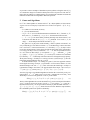
To decide whether Player 1 is winning in a game G, the basic approach consists
in tracing the knowledge of Player 1, represented a set of locations called a cell. The
initial knowledge is the cell s0 = {l0 }. After each round, the knowledge s of Player 1
is updated according to the action a she played and the observation o she receives, to
s′ = posta (s) ∩ γ(o) where posta (s) = {ℓ′ ∈ L | ∃ℓ ∈ s : (ℓ, a, ℓ′ ) ∈ ∆}.
Antichain algorithm. The antichain algorithm is based on the controllable predecessor
operator CPre : 2S → 2S which, given a set of cells q, computes the set of cells q ′ from
which Player 1 can force the game into a cell of q in one round:
CPre(q) = {s ⊆ L | ∃a ∈ Σ · ∀o ∈ Γ : posta (s) ∩ γ(o) ∈ q}.
(1)
The key of the algorithm relies on the fact that CPre(·) preserves downward-closedness.
A set q of cells is downward-closed if, for all s ∈ q, every subset s′ ⊆ s is also in q.
Downward-closed sets q can be represented succinctly by their maximal elements r =
⌈q⌉ = {s ∈ q | ∀s′ ∈ q : s 6⊂ s′ }, which form an antichain. With this representation,
the controllable predecessor operator is defined by
CPre(r) = {s ⊆ L | ∃a ∈ Σ · ∀o ∈ Γ · ∃s′ ∈ r : posta (s) ∩ γ(o) ⊆ s′ } .
(2)
2
Strategy construction. The implementation of the strategy construction is based on [1].
The algorithm of [1] employs antichains to compute winning strategies for imperfectinformation parity games in an efficient and compact way: the procedure is similar to the
classical algorithm of McNaughton [4] and Zielonka [6] for perfect-information parity
games, but, to preserve downwards closure, it avoids the complementation operation
of the classical algorithms by recurring into subgames with an objective obtained as a
boolean combination of reachability, safety, and reduced parity objectives.
Strategy simplification. A strategy in a game with imperfect information can be represented by a set Π = {(s1 , rank1 , a1 ), . . . , (sn , rankn , an )} of triples (si , ranki , aI ) ∈
2L ×N×Σ where si is a cell, and ai is an action. Such a triple assigns action ai to every
cell s ⊆ si ; since a cell s may be contained in many si , we take the triple with minimal
value of ranki . Formally, given the current knowledge s of Player 1, let (si , ranki , ai )
be a triple with minimal rank in Π such that s ⊆ si (such a triple exists if s is a winning
cell); the strategy represented by Π plays the action ai in s.
Our implementation applies the following rules to simplify the strategies and obtain
a compact representation of winning strategies in parity games with imperfect information.
(Rule 1) In a strategy Π, retain only elements that are maximal with respect to the
following order: (s, rank, a) (s′ , rank′ , a′ ) if rank ≤ rank′ and s′ ⊆ s. Intuitively,
the rule specifies that we can delete (s′ , rank′ , a′ ) whenever all cells contained in s′ are
also contained in s; since rank ≤ rank′ , the strategy can always choose (s, rank, a) and
play a.
(Rule 2) In a strategy Π, delete all triples (si , ranki , ai ) such that there exists
(sj , rankj , aj ) ∈ Π (i 6= j) with ai = aj , si ⊆ sj (and hence ranki < rankj by Rule 1),
such that for all (sk , rankk , ak ) ∈ Π, if ranki ≤ rankk < rankj and si ∩ sk 6= ∅, then
ai = ak . Intuitively, the rule specifies that we can delete (si , ranki , ai ) whenever all
cells contained in si are also contained in sj , and the action aj is the same as the action
ai . Moreover, if a cell s ⊆ si is also contained in sk with ranki ≤ rankk < rankj , then
the action played by the strategy is also ak = ai = aj .
3 Implementation
Computing CPre(·) is likely to require time exponential in the number of observations
(a natural decision problem involving CPre(·) is NP-hard [1]). Therefore, it is natural
to let the BDD machinery evaluate the universal quantification over observations in (2).
We present a BDD-based algorithm to compute CPre(·).
Let L = {ℓ1 , . . . , ℓn } be the state space of the game G. A cell s ⊆ L can be
represented by a valuation v of the boolean variables x̄ = x1 , . . . , xn such that ℓi ∈ s
iff v(xi ) = true, for all 1 ≤ i ≤ n. A BDD over x1 , . . . , xn is called a linear encoding,
it encodes a set of cells. A cell s ⊆ L can also be represented by a BDD over boolean
variables ȳ = y1 , . . . , ym with m = ⌈log2 n⌉. This is called a logarithmic encoding, it
encodes a single cell.
We represent the transition relation of G by the n · |Σ| BDDs Ta (ℓi ) (a ∈ Σ,
1 ≤ i ≤ n) with logarithmic encoding over ȳ. So, Ta (ℓi ) represents the set {ℓj |
3
(ℓi , a, ℓj ) ∈ ∆}. The observations Γ = {o1 , . . . , op } are encoded by ⌈log2 p⌉ boolean
variables b0 , b1 , . . . in the BDD BΓ defined by
^
BΓ ≡
b̄ = [j]2 → Cj+1 (ȳ),
0≤j≤p−1
where [j]2 is the binary encoding of j and C1 , . . . , Cp are BDDs that represent the sets
γ(o1 ), . . . , γ(op ) in logarithmic encoding.
Given the antichain q = {s1 , . . . , st }, let Sk (1 ≤ k ≤ t) be the BDDs that encode
the set sk in logarithmic encoding over ȳ. For each a ∈ Σ, we compute the BDD CPa
in linear encoding over x̄ as follows:
_ ^
CPa ≡ ∀b̄ ·
xi → ∀ȳ · Ta (ℓi ) ∧ BΓ → Sk .
1≤k≤t 1≤i≤n
W
Then, we define CP ≡ a∈Σ CPa (q), and we extract the maximal elements in CP(x̄)
as follows, with ω a BDD that encodes the relation of (strict) set inclusion ⊂:
n
n
_
^
xi 6= x′i ,
xi → x′i ∧
ω(x̄, x̄′ ) ≡
i=1
i=1
min
CP
(x̄) ≡ CP(x̄) ∧ ¬∃x̄′ · ω(x̄, x̄′ ) ∧ CP(x̄′ ).
Finally, we construct the antichain CPre(q) as the following set of BDDs in logarithmic
encoding: CPre(q) = {s | ∃v ∈ CPmin : s = {ℓi | v(xi ) = true}}.
Features of the tool. The input of the tool is a file describing the transitions and observations of the game graph. The output is the set of maximal winning cells, and a
winning strategy in compact representation. We have also implemented a simulator to
let the user play against the strategy computed by the tool. The user has to provides an
observation in each round (or may let the tool choose one randomly). The web page of
the tool is http://www.antichains.be/alpaga. We provide the source code,
the executable, an online demo, and several examples. Details of the tool features and
usage are given in the appendix.
References
1. D. Berwanger, K. Chatterjee, L. Doyen, T. A. Henzinger, and S. Raje. Strategy construction
for parity games with imperfect information. Technical Report MTC-REPORT-2008-005,
http://infoscience.epfl.ch/record/125011, EPFL, 2008.
2. K. Chatterjee, L. Doyen, T. A. Henzinger, and J.-F. Raskin. Algorithms for omega-regular
games of incomplete information. Logical Methods in Computer Science, 3(3:4), 2007.
3. K. Chatterjee and T. A. Henzinger. Assume-guarantee synthesis. In Proc. of TACAS, LNCS
4424, pages 261–275. Springer, 2007.
4. R. McNaughton. Infinite games played on finite graphs. Annals of Pure and Applied Logic,
65(2):149–184, 1993.
5. Fabio Somenzi. Cudd: Cu decision diagram package. http://vlsi.colorado.edu/˜fabio/CUDD/.
6. W. Zielonka. Infinite games on finitely coloured graphs with applications to automata on
infinite trees. Theoretical Computer Science, 200:135–183, 1998.
4
Details of Tool Features
4 Practical implementation
In this section we describe the implementation details of the tool Alpaga.
4.1 Programming Language
Alpaga is written in Python, except for the BDD package which is written in C. We
use the CUDD BDD library [5], with its PYCUDD Python binding. There is some
performance overhead in using Python, but we chose it for enhanced readability and to
make the code easy to change. We believe this is important in the context of academic
research, as we expect other researchers to experiment with the tool, tweak the existing
algorithms and add their own.
Alpaga is available for download at http://www.antichains.be/alpaga
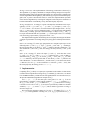
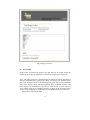
for Linux stations. For convenience, the tool can also be tested through a web interface
(see Fig. 1 for a glimpse to this interface).
4.2 Code architecture
The code consists of four main classes:
1. Game is the main class of Alpaga. It encompasses all necessary information describing a game: BDDs for initial sets, target sets, observations, transition relations.
The class offers two implementations of the controllable predecessors operator:
(a) the“enumerative” CPre implementation which closely follows the definition of
the CPre operator (enumerating labels, states and sets of the antichains, computing desired antichain intersections and unions as it progresses) and (b) the CPre
implementation following the BDD technique explained in Section 3.
Furthermore, the class offers a large set of utility functions to compute, for example, the successors of a set of states, its controllable predecessors, and to manipulate
antichains of sets of states of the game. At a higher level, the class offers methods
to compute strategies for specific kinds of objectives (ReachAndSafe: solving conjunction of reachability and safety objectives, and ReachOrSafe: solving disjunction of reachability and safety objectives). Finally it includes the implementation
of the algorithm of [1] using all previous functions.
2. Parser produces an instance of the class Game from an input file. The parser also
offers a good amount of consistency checking (it checks, for example, that every
state belongs to one and only one observation).
3. Strategy is the class with data structure for strategy representation. The description of a strategy is based on the notion of rank (similar to rank of µ-calculus
formulas), and a strategy maps a cell with a rank to a label and a cell with smaller
rank.
4. StrategyPlayer is the class implementing the interactive mode of Alpaga. It
takes as argument a game and a strategy and allows the user of Alpaga to replay the
strategy interactively (see below).
5
Fig. 1. Alpaga web interface.
4.3 User Manual
In this section we describe the syntax of the input file, how to read the output, the
various options of the tool, and finally we describe the interactive use of the tool.
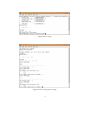
Input. The syntax of the tool is straightforward and follows the formal description of
imperfect information parity games as described in Section 2. Our algorithm solves
games with objectives that are of the following form: parity objectives in conjunction
with a safety objective, along with the disjunction with a reachability objective. The
parity objective can be obtained as a special case when the safe set is the full set of
states, and the target set for reachability objective is empty. In the description below,
we have the safe and target set for the safety and reachability objectives, respectively.
We present the following example:
6
ALPHABET : a
STATES : 1, 2,3
INIT : 1
SAFE : 1,2,3
TARGET : 2
TRANS :
1, 1 , a
1,2, a
2, 3, a
3, 3,a
OBS :
1:1
2:1
3:0
a
a
a
ℓ1
p=1
ℓ2
p=1
a
ℓ3
p=0
The input file describing a parity game with imperfect information is constructed as
follows:
– the sets of labels, states, initial states, safe states, and target states are all specified
on a single line introduced by the corresponding keyword ALPHABET, STATES,
INIT, SAFE or TARGET. The name of the states and labels can be any string accepted by Python that does not include a blank space or the # character (which is
used for comments). However, the keyword SINK is reserved (see below).
– the transition relation is defined on a sequence of lines introduced by the keyword
TRANS on a single line. After the TRANS keyword, each line specifies on a single
line a transition, by giving the initial state, the destination state and the label of the
transition, all separated by commas.
– Finally, the observations and corresponding priorities are specified in a similar fashion. They are introduced by the keyword OBS on a single line. Then follows the
specification of the observations. Each observation is specified on a single line as a
set of comma-separated states, followed by its priority (a positive integer number)
which must be preceded by a colon.
– Blank lines are allowed anywhere as empty comments. Nonempty comments start
with the character # and extend to the end of the line.
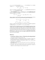
Output. The tool output for our example is in Fig. 2. The winning strategy computed
by the tool is represented by a list of triples (a, rank, s) ∈ Σ × N × 2L where a is an
action, and s is a cell. The strategy is represented in the compact form after applying
Rule 1 and Rule 2 for simplification of strategies. The strategy representation can be
used to find the action to play, given the current knowledge s′ of Player 1 as follows:
play the action a such that (a, rank, s) is a triple in the list with minimal rank such that
s′ ⊆ s (such a triple must exist if s′ is a winning cell).
Tool options. We now describe the various options with which the tool can be used.
alpaga.py [options] file
7
The possible options are the following:
– -h Shows an help message and exits.
– -i After computing a strategy, launches the interactive strategy player which allows
to see how the strategy computed by the tools executes in the game. In this mode,
the tool shows which move is played by the strategy, given the current knowledge
(i.e., a set of states in which the player can be sure that the game is - the initial
knowledge is the set of initial states). Then the tool allows to choose the next observations among the observations that are compatible with the current knowledge.
– -e Uses the enumerative CPre in all computations. There are two different implementations for the controllable predecessor operator (CPre), one temporarily using
a linear encoding of the resulting antichain for the time of the computation, and an
enumerative algorithm following closely the definition of the CPre operator.
– -n Turns off the totalization of the transition relation. By default, Alpaga completes
the transition relation so that it becomes total, which means that a transition of
every label exists from each state. Therefore, Alpaga first adds a state named SINK
with priority 1 (corresponding to a new observation), from which every label loops
back to SINK, and then adds a transition
s, SINK, lab
for each pair (s, lab) such that there does not exist a transition from state s on label
lab. Note that the name SINK is reserved.
– -r Turns on the display of stack traces in case of error.
– -s Turns off the simplification of the strategies before display.
– -t Displays computation times, which includes time for parsing the file (and constructing the initial BDDs), time for initializing the linear encoding, for computing
a strategy, and for simplifying that strategy.
– -v Turns on the display of warnings, which mainly list the transitions added by the
totalization procedure.
Interactive mode. After computing a strategy for a parity game, the tool can switch to
interactive mode, where the user can “replay” the strategy, to check that the modelization was correct. The user of Alpaga plays the role of Player 2, choosing the observation
among the compatible observations available, and getting the resulting knowledge of
player 1 and which move she will play.
Practically, in interactive mode, type help for the list of commands: the standard
way for playing a strategy is the following: launch alpaga with option -i, type go at the
interactive prompt, type the number of an observation, type enter twice, repeat. Fig. 3
shows an interactive Alpaga session.
5 Example: mutual-exclusion protocol
We demonstrate the use of games with imperfect information to synthesize reactive
programs in distributed systems. We consider the design of a mutual-exclusion protocol
8
Fig. 2. Output of Alpaga.
Fig. 3. Interactive strategy player of Alpaga.
9
do {
unbounded_wait;
flag[2]:=true;
turn:=1;
do {
unbounded_wait;
flag[1]:=true;
turn:=2;
|
|
|
|
|
|
|
|
while(flag[1]) nop;
while(flag[2]) nop;
while(turn=1) nop;
while(turn=2) nop;
while(flag[1] & turn=2)
while(flag[1] & turn=1)
while(flag[2] & turn=1)
while(flag[2] & turn=2)
nop;
nop;
nop;
nop;
(C1) while(flag[1] & turn=1) nop;
(C2)
(C3)
(C4)
(C5)
(C6)
(C7)
(C8)
fin_wait; // Critical section
flag[2]:=false;
} while(true)
fin_wait; // Critical section
flag[1]:=false;
} while(true)
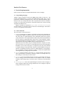
Fig. 4. Mutual-exclusion protocol synthesis.
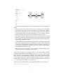
for two processes, following the lines of [3]. We assume that one process (on the right
in Fig. 4) is completely specified. The second process (on the left in Fig. 4) has freedom
of choice in line 4. It can use one of 8 possible conditions C1–C8 to guard the entry
to its critical section in line 5. The boolean variables flag[1] and flag[2] are used to
place a request to enter the critical section. They are both visible to each process. The
variable turn is visible and can be written by the two processes. Thus, all variables are
visible to the left process, except the program counter of the right process.
There is also some nondeterminism in the length of the delays in lines 1 and 5 of
the two processes. The processes are free to request or not the critical section and thus
may wait for an arbitrary amount of time in line 1 (as indicated by unbounded wait),
but they have to leave the critical section within a finite amount of time (as indicated by
fin wait). In the game model, the length of the delay is chosen by the adversary.
Finally, each computation step is assigned to one of the two processes by a scheduler. We require that the scheduler is fair, i.e. it assigns computation steps to both processes infinitely often. In our game model, we encode all fair schedulers by allowing
each process to execute an arbitrary finite number of steps, before releasing the turn
to the other process. Again, the actual number of computation steps assigned to each
process is chosen by the adversary.
The mutual exclusion requirement (that the processes are never simultaneously in
their critical section) and the starvation freedom requirement (that whenever the left
process requests to enter the critical section, then it will eventually enter it) can be
encoded using three priorities.
When solving this game with our tool, we find that Player 1 is winning, and that
choosing C8 is a winning strategy.
10