1
ST200 Radar Evaluation System
User Manual
© RFbeam Microwave GmbH www.rfbeam.ch
January 2013
Page 1/27
User Manual
ST200 Evaluation System
Features
Supports Doppler, FMCW, FSK, Monopulse
USB Interface to Host Computer
Onboard Low Noise Power Supplies
Connectors for Different Radar Devices
Amplifiers for Native Doppler Transceivers
High Performance 16Bit Data Processing
250kSamples/s ADC and DAC
Compact and Rugged Construction
Powerful Signal Explorer PC Software
NI LabVIEW ® DAQmx USB Interface
•
•
•
•
•
•
•
•
•
•
Applications
-
Evaluation of Advanced Shortrange Radar Applications
Development of Own Data Processing Algorithms
Signal Analysis and Logging
Learning and Exploring Radar Basics
Description
ST200 is a 16Bit data acquisition and processing system with a total 250k/s sampling rate. It contains
all hardware necessary for acquiring Radar signals of RFbeam Transceivers.
ST200 contains a motherboard with power supply, amplifiers and I/O connectors. Data acquisition is
performed by a NI-USB-6211 16Bit multifunction DAQ module from National Instruments mounted on
the backside.
The easy to handle RFbeam Signal Explorer software features many basic Radar functions including
an exciting FSK (Frequency Shift Keying) operation mode for high resolution distance measurements
of moving objects.
ST200 Block Diagram
Radar Connectors:
X1: General purpose I/O
X2: Mixed I/O
X3: 4 Channel An. Inputs
X4: 2 Channel An. Inputs
X5: 2 Channel An. Inputs
Computer Interface:
X9: USB PC Port
Power:
X10: Optional DC In
X11: Low Noise DC Out
© RFbeam Microwave GmbH www.rfbeam.ch
January, 2013
Page 2/27
User Manual
ST200 Evaluation System
Getting Started
Please install software prior to connect ST200 to the USB port.
Equipment Needed
•
•
•
•
•
ST200 Hardware
ST200 Signal Explorer Software Installer on CD, USB stick or downloaded on HD
USB cable
K-LC2 sensor connected to connector X5
PC running on Windows xp or never
Installing Signal Explorer Software
ST200 software comes with a setup procedure containing all necessary components into one single
package:
•
•
•
RFbeam ST200 Signal Explorer Software
National Instruments DAQmx ® driver software
National Instruments LabVIEW ® runtime systerm
1. Start RFbeam Signal Explorer setup.exe from your intallation media
If your computer does not already contain a LabVIEW runtime engine and DAQmx driver, you
will be prompted to accept licences of National Instruments.
2. If possible, accept all default program locations. Troubleshooting will be simplified like this.
3. Please be patient while LabVIEW runtime system and DAQmx driver are being installed.
This may take some minutes...
4. Restart your computer, if asked so.
5. You will find SignalViewer under START->PROGRAMS->RFbeam->Signal Explorer and a
shortcut icon on the Desktop.
© RFbeam Microwave GmbH www.rfbeam.ch
January, 2013
Page 3/27
User Manual
ST200 Evaluation System
Test Configuration and Go!
We will now take a first impression by using the Doppler mode and observe movement of persons.
Please refer to the screen shot in Fig. 1
1. Plug in a K-LC2 radar sensor into connector X5 of the ST200.
2. Connect ST200 hardware to you computer. There should appear a “New USB Hardware
Found” message from Windows.
3. Windows will probably ask you for a hardware driver. Select to find it aoutomatically.
4. Start SignalExporer under START->PROGRAMS->RFbeam->SignalExplorer
After some seconds the main screen of the Signal Explorer should appear.
5. Select the most important controls according to Fig. 1 below.
6. Drag all 3 cursors as shown in Fig. 1 . If cursors are not visible, press cursor "Reset" button.
7. Now move your hands in front of the K-LC2 sensor. You will see the frequency and speed in
the upper graph and the time signal (oscilloscope) in the bottom graph.
8. Explore and become familiar with the effect of the 3 cursors.
9. Try to switch to Doppler-Phase screen by using the left tab in the bottom half of the screen.
You will see the direction of your movement (Cursors must be set according to Fig. 1 ).
Sensor configuration
Detection area
defined by 3 cursors
Logarithmic display
Channel for FFT
Reset cursors to
visible area
Time domain modes
Filter settings for time
domain
Channels to show
Y-range
Y-range
Fig. 1: Start Screen. Try to set all marked controls according to this figure
© RFbeam Microwave GmbH www.rfbeam.ch
January, 2013
Page 4/27
User Manual
ST200 Evaluation System
ST200 Hardware
ST200 consists of a mother board and a 16 Bit USB data acquisition system with 250kHz sampling
rate. The mother board contains 5V and 3.3V low noise power supplies and analog buffers and
amplifiers.
Power Supplies
Pre-Amps
FM Level Shifters
X9
X10
JP1 -> X1
3.3V / 5V
JP2 -> X2
Dig. I/O
JP3 -> X2,3
3.3V / 5V
JP4 -> X4,5
3.3V / 5V
X11
X1
X2
X3
X4
X5
Fig. 2: Connector Arrangement
Sensor Connectors:
X1: General purpose I/O
X2: Mixed I/O
X3: 4 Channel An. Inputs
X4: 2 Channel An. Inputs
X5: 2 Channel An. Inputs
Computer Interface:
X9: USB PC Port
Power:
X10: Optional DC In
X11: Low Noise DC Out
Fig. 3: Block Diagram
© RFbeam Microwave GmbH www.rfbeam.ch
January, 2013
Page 5/27
User Manual
ST200 Evaluation System
Typical Sensor Connections
Please refer to Fig. 3 and to chapter Sensor Connectors for more details on tzhe connectors.
Sensors with higher current consumption (>120mA like K-MC4) need more power than USB can
deliver.
An external DC 12V power supply with >0.5A should be plugged into X10 of the ST200 system.
K-LCx Series → X5 or X4
Sensors of the K-LCx series with no internal amplifiers can directly be plugged into X5.
For remote connecting K-LCx sensors, a 6 pin ribbon flat cable my be connected to X4.
X5 or X4 provide 2 channels with amplifiers.
K-MCx and K-HC1 Series → X3
K-MCx sensors provide internal amplifiers and are typically connected to X3.
X3 provides 2 channels and is directrly routed to the DAQ system.
Notes:
- K-HC1 needs an own, separate power supply and a special adapter cable.
- K-MC4 can only be operated with an external 12VDC power supply connnected to X10.
Other Sensors
Please contact RFbeam for instructions on connecting special sensors.
© RFbeam Microwave GmbH www.rfbeam.ch
January, 2013
Page 6/27
User Manual
ST200 Evaluation System
Signal Explorer Software
Overview
Getting Help
Most controls and readouts provide a context help on mouse over.
Select Help - Show ContextHelp from main menu. This opens a floating window containing a brief
description of the object pointed by the mouse cursor.
Operation Modes
ST200 Signal Explorer provides 3 main operation modes:
•
Doppler Mode: Speed and direction measurements
•
FMCW Mode: Distance measurements of statical and moving objects
•
FSK Mode:
Distance measurements with high resolution for moving objets
User interface includes selecting of operation modes and sensor types, setting of filter types and
bandwidth, sampling rates, graphical representation of signals in time and frequency.
User inteface screen is devided into 3 sections:
General Section
Operation Section
Recorder Section
Fig. 4: Screen Sections
© RFbeam Microwave GmbH www.rfbeam.ch
January, 2013
Page 7/27
User Manual
ST200 Evaluation System
General Section
Settings and readouts in the general screen section (see Fig. 4) are accessible in all operation modes.
Readouts
Samples:
Rate:
Loop Time:
loop time=
Number of samples per channel as input for the signal processing (FFT).
ADC sampling rate per channel.
Time to read the samples defined in the selected configuration. It is calculated by
number of samples
samplingRate
Configurations Selector
Many key settings are stored as so called configurations. Existing configurations may be selected at
any time. After selecting, Signal Explorer jumps back into operation mode Doppler.
Configuration naming convention:
K-LC2_X4-5_IQH.cfg
|
| |_ connector inputs
|
|____ connector name(s) (refer to chapter Sensor Connectors)
|__________ sensor type
Configurations Setup
You may alter or copy existing configurations. New configurations may be generated.
Refer to chapter Settings for more details.
Operation Section
This is the real time signal section (see Fig. 4).
Select the operation mode with the horizontal tabs on the top. Some modes allow selecting sub-modes
by the vertical tabs in the bottom left part of the operation section.
Recorder Section
ST200 Signal Explorer allows real time recording and playback of signals captured in the Doppler and
in the FSK mode.
© RFbeam Microwave GmbH www.rfbeam.ch
January, 2013
Page 8/27
User Manual
ST200 Evaluation System
Using Signal Explorer Software
Doppler Mode
About Doppler Radar
A more precise tiltle would be 'CW (Continuous Wave) Doppler Radar', when using RFbeam Radar
sensors. These sensors do not produce pulses, but send continuously in the K-band (24.125 GHz ).
The sensors are also called Radar transceivers, because they include a Transmitter and a Receiver.
Doppler Radar is used to detect moving objects and evaluate their velocity. More details on the
principle can be read here:
http://en.wikipedia.org/wiki/Doppler_radar
http://www.radartutorial.eu/11.coherent/co06.en.html
Tx
Rx
K-LC1a
IF output
FM Input
Fig. 5: Typical Radar Transceiver
RFbeam Radar transceivers return a so called IF signal,
that is a mixing product of the transmitted (Tx) and the
received (Rx) frequency. An moving object generates a
slightly higher or lower frequency at the receiver. The IF
signal is the absolute value of the difference between
transmitted and received frequency.
These transceivers operate in the CW (Continuous Wave)
mode as opposed to the pulse radars, that measure time
of flight. CW radars can operate with very low transmit
power (< 20dBm resp. 100mW).
Calculating the Doppler frequency
f d=
2⋅ f Tx⋅v
⋅cos α
c0
(1)
or
v=
c0⋅ f d
2⋅ f Tx⋅cos α
(2)
fd
fTx
c0
v
α
Doppler frequency
Transmit frequency (24GHz)
Speed of light (3 * 108 m/s)
Object speed in m/s
Angle between beam and object moving direction
At a transmit frequency of fTx = 24.125GHz we get a Doppler frequency for a moving object at the IF
output of
f d =v [km/h]⋅44Hz⋅cos α or
α
moving
object
Radar sensor
Fig. 6: Definition of angle α
f d =v [m/s ]⋅161Hz⋅cos α
(4)
Angle α reduces the measured speed by a factor of cos α.
This angle varies with the distance of the object.
To evaluate the correct speed, you need a trigger criteria at a
known point. This can be accomplished by measuring the
distance with the radar sensor (e.g. using FSK technology) or
by measuring the angle using a monopulse radar such as
K-MC4.
© RFbeam Microwave GmbH www.rfbeam.ch
January, 2013
Page 9/27
User Manual
ST200 Evaluation System
ST200 Doppler Mode
Note the difference between logarithmic (upper figure) and linear (bottom figure) FFT display. Smaller
peaks in logarithmic display disappear in linear display.
Logarithmic/Linear
display
Cursor high freq. limit
Cursor low freq. limit
Low amplitude limit
Filter for time signal
bandwidth
Reset cursors to visible
area
Fig. 7: Logarithmic FFT scale
Note the difference: in linear mode, small signals and noise disappear.
Linear display
Fig. 8: Linear FFT scale
Remember to reset cursors after switching between logarithmic and linear mode.
© RFbeam Microwave GmbH www.rfbeam.ch
January, 2013
Page 10/27
User Manual
ST200 Evaluation System
Chart Modes
Besides the classical scope modes, ST200 allows “chart” modes for viewing slow signals.
Zooming and shifting charts
Data for the charts come from the signal buffer. Scaling is performed on display level and not on signal
level. This allows scrolling and zooming.
Charts may be zoomed by changing the Y range and/or by changing the horizontal chart speed.
Charts may be “freezed”. Freezed charts may be horizontally scrolled over a history of around 1 million
samples.
Signal chart mode
The “Signal chart mode” (Fig. 9) is similar to the scope mode, but writes the signal on a slow moving
chart. This is useful for visualization of very slow signals.
Decimation factor
Resulting sampling rate
Fig. 9: Signal chart mode. Slow chart, high frequency → Envelope chart
You may (and should) downsample the signal, so that not all the signal buffer will be written to the
chart. Set the decimation factor to the highest possible value, but smaller than the number of samples
(in this example 8192) defined in the configuration.
This process is called decimation or resampling. It includes anti aliasing adapted to the new sampling
rate:
f s ( chart)=
sampling rate per channel
decimation factor
→ Example in Fig. 9
125kHz
=31.25kHz
4
The reduced sampling rate limits upper frequency in chart to 0.4 * fu = 12.5kHz in our example.
© RFbeam Microwave GmbH www.rfbeam.ch
January, 2013
Page 11/27
User Manual
ST200 Evaluation System
Signal chart mode - very slow signals
Fig. 10: Signal chart mode, very low frequency (record of human breathing)
Note: "Suppress DC" checkbox should be uncheckt. Otherwise slow signal will be interpreted as DC
and removed or distorted.
RMS chart Mode
The “RMS chart mode” traces the RMS amplitude of the selected peak in a chart.
Fig. 11: RMS chart mode. Traces the selected peak's RMS amplitude
Fig. 11 shows an RMS amplitude chart of a selected peak. The amplitude drops to 0, as soon as the
peak in the FFT falls outside the selected area. In our example, it dropped under the minimum level
selected by the horizontal cursor.
© RFbeam Microwave GmbH www.rfbeam.ch
January, 2013
Page 12/27
User Manual
ST200 Evaluation System
Exploring the phase relation
Phase relaion bewtween two channels can be evaluated by using "cross FFT" algorithms (Fig. 12) or
by using "complex FFT" (Fig. 13).
I and Q channel selected
Target is approaching
Target is receding
Phase display
Fig. 12: Display I and Q phase relation to evaluate moving direction
Complex FFT
receding targets
approaching targets
Time signal display
Fig. 13: Complex FFT with one approaching target: peak on right side
© RFbeam Microwave GmbH www.rfbeam.ch
January, 2013
Page 13/27
User Manual
ST200 Evaluation System
FMCW Mode
About FMCW
FMCW stands for Frequency Modulated Continuous Wave. This technique allows detection of
stationary objects. FMCW needs Radar sensors with an FM input. This input accepts a voltage that
causes a frequency change. There are also sensors with digital frequency control based on digital PLL
designs. Modulation depth is normally a very small amount of the carrier frequency. In the K-band,
most countries allow a maximum frequency range of 250MHz.
Descfription of many effects such as velocity-range unambiguities go beyond the scope of this paper.
Please refer to Radar literature for more detailed explanations of FMCW and FSK techniques.
Sawtooth Modulation
Transmit frequency is modulated by a linear ramp. Fig. 14 shows a typical signal fRx returned by
stationary and constantly moving objects. Note, that the difference frequency fb is constant throughout
nearly the whole ramp time.
At the output of the Radar transceiver we get the low frequency signal fb called beat frequency. This is
the result of mixing (=multiplying) transmitted and received frequencies (refer to Fig. 5).
Sawtooth modulation has important disadvantages:
•
It is very difficult to get reliable results for moving objects
•
The very sharp down ramp can disturb the amplified signals (ringing, saturation)
Returned echo from stationary object
f
fM
tp
fTx
fRx
fb
TM
t
Modulation depth
Modulation period
Transmitted frequency
Received frequency
Signal propagation time (time of flight)
Beat frequency fTx - fRx
Doppler shift frequency
Returned echo from moving object
f
fM
fM
TM
fTx
fRx
tp
fb
fD
tp
fTx
fRx
Received frequency fRx is shifted by fD .
This is the Doppler frequency caused by a
receding object moving at a constant speed.
fb
fD
TM
t
Fig. 14: Sawtooth modulation
Above: Stationary object, Below: Moving object
Distance can be calculated as follows:
c f
R= 0 ⋅ b ⋅T M
2 fM
(5)
© RFbeam Microwave GmbH www.rfbeam.ch
For legend refer to Fig. 14 above
R Range, distance to target
c0 Speed of light (3 * 108 m/s)
January, 2013
Page 14/27
User Manual
ST200 Evaluation System
Triangle Modulation
Transmit frequency is modulated by a linear up and down ramp. Fig. 15 shows a typical signal fRx
returned by stationary and constantly moving objects. Note, that the difference frequency fb is constant
throughout nearly the whole ramp time.
At the output of the Radar transceiver we get the a low frequency signal fb called beat frequency. This
is the result of mixing (=multiplying) transmitted and received frequencies (refer to Fig. 5).
Returned echo from stationary object
f
tp
fM
fTx
fb
fRx
TM
t
Modulation depth
Modulation period
Transmitted frequency
Received frequency
Signal propagation time (time of flight)
Beat frequency fTx - fRx
Doppler shift frequency
Returned echo from moving object
f
fM
fM
TM
fTx
fRx
tp
fb
fD
fTx
Received frequency fRx is shifted by fD .
This is the Doppler frequency caused by a
receding object moving at a constant speed.
fb2
fb1
fRx
TM
fD
t
By measuring during up and down ramp,
Doppler frequency fD is the diffence between
fb1 and fb2 .
Fig. 15: Triangle modulation
Above: Stationary object, Below: Moving object
Distance can be calculated as follows:
c f T
R= 0 ⋅ b ⋅ M
2 fM 2
(7)
For legend refer to Fig. 15 above
R Range, distance to target
c0 Speed of light (3 * 108 m/s)
(8)
For legend refer to Fig. 15 above
Rmax
Max. unambiguos target distance
c0
Speed of light (3 * 108 m/s)
Maximum unambiguous range:
c T
Rmax = 0 ⋅ M
2 2
Advantages of triangle modulation:
•
Doppler frequency can be determined
•
IF amplifiers are less stressed than with sawtooth modulation
Advanced FMCW Modulation Techniques
Triangle modulation may be extended with phase of constant frequency to allow Doppler detection.
You find examples in chapter Exploring FMCW.
© RFbeam Microwave GmbH www.rfbeam.ch
January, 2013
Page 15/27
User Manual
ST200 Evaluation System
Distance and Resolution
In K-Band (24GHz), maximum allowed frequency modulation depth fM is < 250MHz. We also have to
take in account tolerances and temperature influences. This limits the usable frequency shift fM to
typically 150MHz
For measuring fb to evaluate distance we need at least one period of fb during TM , range resolution is
limited to
Rmin =
c0
38 m/s
=
=0.6m
2⋅ f M 2⋅250MHz
(6)
This is a theoretical value, because we have to
take in account drifts and tolerances in order to
stay in the allowed frequency band.
Working with the more realistic value of fM = 150MHz, we get a minimum distance and resolution of
R = 1m .
Resolution may be enhanced by using phase conditions, correlation and other sophisticated
algorithms.
Real World EffectsSelf-Mixing Crosstalk
FM modulation with radar transceivers can produce side effects. Most annoying effect is caused by the
feed through of the modulation signal to the IF output. This effect is caused by the limited isolation
between transmitter and receiver path and can be called self-mixing. This effect limits the minimal
detectable distance. This signal also limits the maximum signal amplification.
Target
a) VCO modulation signal
c) FFT of the signal sensor output signal b)
Left picture b) shows the I and Q signals of a KMC1 sensor. Target has a distance of 5m. Self
mixing signal is much higher than the reflected
sinus signal of the target.
FFT in picture c) shows, that target signal is very
close to the self mixing signal.
b) Resulting sensor output with target in 5m
Fig. 16: FMCW effect of self mixing
Similar effects may be caused by poor quality of the cover in front of the sensor antenna. The cover is
often called RADOM (from Radar Dome). The reason is different reflectivity at different frequencies.
Please contact RFbeam for more informations on Radom.
© RFbeam Microwave GmbH www.rfbeam.ch
January, 2013
Page 16/27
User Manual
ST200 Evaluation System
Linearity
Non-linearity reduces resolution and sensitivity in FMCW ranging applications.
Linearity of the frequency ramps is crucial for reliable distance information. Varactor based open loop
oscillators suffer of non linearities, that must be corrected by the FMCW VCO voltage generator.
RFbeam Signal Explorer offers tools to calculate and compensate non linearities. We will explain this
later.
Exploring FMCW
FMCW may be best explored by using RFbeam K-MCx sensors. These sensors have enough
sensitivity and beam focussing to demonstrate FMCW for many applications.
Best experience can be obtained by placing the Radar sensor outdoor. Fig. 17 shows an
example of a signal from a sensor placed outside an office window.
Please note that some window types may absorb Radar signals, if they contain metallic
components.
No Doppler phase:
Readout is disabled
Distance at cursor position
Object in 39.5m
VCO ramp
Freq ramp
VCO Linearization
ON/OFF
VCO Linearization
Tool
Fig. 17: ST200 FMCW Screen Overview using a K-MC1 sensor.
Bottom right graph in Fig. 17 demonstrates a calculated VCO ramp (yellow) to get a linear frequency
ramp (blue). For more details on linearization refer to chapter FM Linearization.
Doppler FFT is displayed only, if VCO ramp contains a third, constant frequency block (called "3blocks" FM Type).
In FMCW mode, the number of samples is defined by the definition of the VCO ramp. Refer to
chapter FM Ramp Definitions.
Try using "Learn" button to mask out the momentary FMCW objects in FFT readout.
Select then "Diff" display. In this mode with linear FFT (Vrms) readout, be sure to extend
range of Y axis to negative values also.
This allows better viewing changed situations in the environment.
© RFbeam Microwave GmbH www.rfbeam.ch
January, 2013
Page 17/27
User Manual
ST200 Evaluation System
FSK Mode
FSK stands for Frequency Shift Keying. FSK uses two discrete carrier frequencies fa and fb, (Fig. 18)
while FMCW uses linear ramps.
For each carrier frequency, separate IF signals must be sampled in order to get 2 buffers for separate
FFT processing.
Due to the very small step fa - fb a moving target will apear at the nearly the same Doppler frequency
at both carriers, but with a different phase (Fig. 19) .
Phase shift due to the modulation timing and sampling must also be taken into account.
fa
fb
txa
txb
f
fa
Ta
Tb
fb
txa txb txa txb
txa txb
t
Fig. 18: FSK modulation scheme
IF(txa)
Carrier Frequency a
Carrier Frequency b
Sampling point for Doppler a
Sampling point for Doppler b
Switching must be performed at a sampling rate
high enough to meeting the Nyquist criteria for the
Doppler signal acquisition.
IF(txa) Sensor output signal at Carrier Frequency fa
IF(txb) Sensor output signal at Carrier Frequency fb
IF(txb)
Doppler signals of the same moving target have
same frequency, but are phase shifted by Δφ
For both IF signals, phase must be determined at
the spectral peak of the object.
Fig. 19: Resulting Doppler frequencies
R=
c 0⋅Δ φ
4 π⋅( f a − f b)
(7)
Δφ Phase shift of IF(txa) and IF(txb)
φ ranges from 0 to 180°
Sign of φ indicates moving direction
The smaller the frequency step, the higher the maximum range.
With a frequency step of 1 MHz, you will get unambigous distance range of 75m.
• FSK can only be used for moving objects
• Multiple objects at different speeds may be detected
• Distance resolution depends manly on signal processing and is not limited by the carrier
bandwidth limitations
• FSK has the advantage of simple modulation and does not suffer from linearity problems
• VCO signal generation is simple, but sampling and phase measurement is challenging
© RFbeam Microwave GmbH www.rfbeam.ch
January, 2013
Page 18/27
User Manual
ST200 Evaluation System
Exploring FSK
The power of FSK may be best explored by using the simple K-LC1a or other K-LCx series
sensors. You may check the functionality by walking around in front of these sensors.
Please note, that FSK allows even moving direction detection with the 1 channel K-LC1.
Technical Background
ST200 generates a continuous rectangular signal stream at the VCO input of the Radar sensor. With a
strict and jitter free clock, two signal buffers, one for fa, one for fb. (see Fig. 18), are generated from the
sensor IF output. Sampling rate of each buffer is normally ¼ of the sampling rate of the analog output.
This rate may be changed using the setup feature described in chapter Configurations Setup.
Both buffers are fed into the 2 inputs of a cross FFT, that allows measuring the phase for each
spectral line.
Phase (=distance) is displayed on Signal Explorer for the highest level spectral peak only. But FSK
would allows detecting distances of many targets with different speeds.
FSK is possible even with RFbeam's low cost sensor K-LC1a.
Select capturing area
with cursors
Frequency step
Hold time if speed = 0
standing still
→ hold time
Distance chart speed
Fig. 20: FSK using K-LC1a: moving person, stopping for 1 second
Recording in FSK mode is possible. This allows analyzing situations under laboratory conditions.
Please select an appropriate area by means of the cursors in the FFT graph.
Phase calculation can be performed for each single frequency. In ST200, only the highest
peak in the capturing area is taken in account.
© RFbeam Microwave GmbH www.rfbeam.ch
January, 2013
Page 19/27
User Manual
ST200 Evaluation System
Recording and Playback
ST100 allows recording and playing back Radar signals. Data is stored in multichannel TDMS files
according to the National Instruments ® standard. There is no compression. Sampling rate in the file
corresponds to the main sampling rate.
Following items are stored in the TDMS file:
Channel related:
- Channel (= Signal) Name
- Data length
- Samples/cycle
- Date/time of recording start
Administration:
- Sensor Name
- Author (user name of PC)
- Notes (not used yet)
- Configuration Name
- System Mode (Doppler, FSK)
FMCW recording is not supported in the current Signal Explorer version
Recording produces very long filels, depending on sampling rate, number of channels and
recording duration.
Limiting file size
You may limit stream file size with different method:
1. Limit size by file size
2. Limit size by recording time
3. Split recording into multiple, size limited files. Multiple files will be numbered automatically.
Fig. 21: Unlimited stream
Fig. 22: 4 files limited to 10MB each
Fig. 23: Resulting files in Multi File mode selected as in Fig. 22
Please find more details on TDMS file format on http://zone.ni.com/devzone/cda/tut/p/id/3727.
© RFbeam Microwave GmbH www.rfbeam.ch
January, 2013
Page 20/27
User Manual
ST200 Evaluation System
Settings
Configurations
ST200 settings including sensor type are collected in configurations. You may generate as many
configurations as you need.
Configurations Setup
You may alter or copy existing configurations. New configurations may be generated.
2
1
3
4
9
5
6
7
8
10
Select predefined configurations from list
box.
A configuration contains and defines:
•
Sensor type
•
Assigned connector
•
Sampling per channel
•
FSK period
Existing configurations may be overwritten
(be careful!) or new ones may be generated.
Fig. 24: Configuration Setup Dialog
Element
Description
1
Configuration selector
Select an existing configuration for viewing details or changing sampling parameters.
2
New configuration button
Select a new configuration based on the selected one.
3
Delete
Remove selcted configuration
4
Connectors
Select connector. Refer to chapter Sensor Connectors.
5
Devices
Select an existing sensor as defined by Radar Sensor Specification electronic datasheet.
6
Sampling Rate
ADC sampling rate per channel.
Maximum is 250ks devided by number of chanels.
7
Samples per channel
Number of samples per channel as input for the signal processing (FFT).
8
FSK period
Period of one FSK cycle in samples. Minimum period is 4.
-> 2 samples per carrier frequency
9
Connector information
Key data of the selected connector (not changable)
10
Save button
Active, whenever you have made changes
If generating new configurations, the system proposes a name root as follows.
You may change or complete it.
K-LC2_X4-5_IQH.cfg
|
| |_ connector inputs
|
|____ connector name(s) (refer to chapter Sensor Connectors)
|__________ sensor type
Please do not change existing configurations, if you are not 100% sure about what you are
doing. Unexpected behaviour may occur at inaccurate settings.
xx_default configurations can not be deleted.
© RFbeam Microwave GmbH www.rfbeam.ch
January, 2013
Page 21/27
User Manual
ST200 Evaluation System
Radar Sensor Specification
Radar Sensor specification makes part of the configuration. Each sensor is defined by an electronic
datasheet sensorname.ini.
[Comment]
comment =
for future use
[ModuleConfig]
stereo = TRUE
MonoPulse = FALSE
RxChannels = 1
These items define general sensor achitecture
[VCO]
V_fmin = 1.000000
V_f0 = 5.000000
V_fmax = 10.000000
V_FMmax = 10
f_min = 24.036000
f_0 = 24.105000
f_max = 24.230000
Items affected automatically by FM Linearization
Minimal VCO voltage
Interpolation point at approx. ½ VCO range
Maximal VCO voltage
for future use
Frequency @ VCO voltage V_fmin
Frequency @ VCO voltage V_f0
Frequency @ VCO voltage V_fmax
Fig. 25: MC1.ini: Typical electronic datasheet for K-MC1
Naming convention
When creating a new configuration, this filename defines the sensor type. Example:
File MC1.ini → device name MC1.
Storage location
All device specifications are stored under \ModuleSettings as explained in chapter Working Files.
Adapting Existing Devices
Only items to change are the VCO characteristics. Changing the VCO data automatically affect the
corresponding sensorname.ini file.
Generating New Devices
You may define new sensors by copying an existing file and editing by an ASCII editor like notepad or
similar.
VCO values must be known and can be evaluated by using RFbeam K-TS1 test system
(http://rfbeam.ch/fileadmin/downloads/datasheets/Datasheet_K-TS1.pdf)
© RFbeam Microwave GmbH www.rfbeam.ch
January, 2013
Page 22/27
User Manual
ST200 Evaluation System
FM Ramp Definitions
FM ramp is defined in files:
[FMCW_Spec]
UserWavePath =
//Number of Samples
UpRamp = 2048
DnRamp = 2048
Doppler = 4096
for future use
Number of samples for up-chirp
Number of samples for down-chirp
Number of samples for doppler (0 = no doppler)
Fig. 26: FMCW ramp description example '3-blocks-8192.ini'
This generates an FMCW period of total 8192 samples:
Absolute voltage levels for 100% amplitude are given by the Radar sensor specification
described in chapter Radar Sensor Specification.
Frequency range depends on Radar Sensor Specification
•
Linearity compensation depends on FM Linearization
•
Sampling rate depends on configuration settings described in chapter Configurations.
•
•
FM Linearization
ST200 provides a tool "VCO-Lin" for interpolating the VCO characteristic from 3 known points.
Output may be exported as csv file and can be used as table for your own FMCW system.
Call the tool by the [Set VCO] button in FMCW mode (see Fig. 17). You may get the 3 frequency
points by measuring the sensor with RFbeam's K-TS1 test system.
VCO-Lin interpolates 3 points of the VCO courve to as many points (samples) as you wish.
2
3
6
1:
Enter 3 value pairs Vvco - f[GHz].
These points are related to the Radar Sensor
Specification
2:
Select type of output:
Frequency vs VCO or
VCO vs. frequency
3:
Number of interpolation poins
4:
Dragable cursor
5:
Polynom informations
6:
Numeric output table
7:
Export output table to a CSV file.
1
4
5
7
© RFbeam Microwave GmbH www.rfbeam.ch
January, 2013
Page 23/27
User Manual
ST200 Evaluation System
File and Directory Organisation
System Files
The files below must not be edited by the user. Configuration files found below are default files and
will be copied to user storage space during installation.
[Programdir]\RFbeam\ST200_SignalExplorer\
ST200.exe
vital program files
...
Configurations\
AI_Config.ini
1)
K-LC1_default.cfg
K-LC1_X4-4IH.cfg
***.cfg
configuration files
factory settings
will be copied to user space during installation
FMCW-Settings\
3-blocks_8192.ini
Triangle_4096.ini
***.ini
FMCW wave descriptions
factory settings
will be copied to user space during installation
ModuleSettings\
K-LC1.ini
K-LC2.ini
***.ini
Radar sensor descriptions
factory settings
will be copied to user space during installation
Note 1) : AI_Config.ini contains hardware informations on the ST200 platform
Working Files
During installation, setup procedure copies the files below to user directories. Location depends on
operating system. These files should not be changed directly, but are affected by the different setup
options of Signal Explorer.
Windows xp
C:\Documents and Settings\user name\Local Settings\AppData\RFbeam\ST200
C:\Dokumente und Einstellungen\Benutzer name\Lokale
Einstellungen\Anwendungsdaten\RFbeam\ST200
Windows Vista, Windows 7
C:\Users\user name\AppData\Local\RFbeam\ST200\
Note: this directory may be hidden. For accessing, you need to change folder settings to "Show hidden
files“.
Appstats.ini
Statistics and installation history
System.ini
Last panel control settings
Configurations\
AI_Config.ini
1)
K-LC1_default.cfg
K-LC1_X4-4IH.cfg
***.cfg
configuration files
contain settings stored from Configurations Setup
FMCW-Settings\
3-blocks_8192.ini
Triangle_4096.ini
***.ini
FMCW wave descriptions
ModuleSettings\
K-LC1.ini
K-LC2.ini
***.ini
Radar sensor descriptions
© RFbeam Microwave GmbH www.rfbeam.ch
January, 2013
Page 24/27
User Manual
ST200 Evaluation System
Sensor Connectors
X1 Universal I/O
The universal connector X1 contains three analog inputs, two analog outputs and four digital in- and
outputs for individual use.
X1 Pin Configuration
Pin
1
2
3
4
5
6
7
8
9
10
11
12
13
14
15
16
17
18
19
20
Signal
AI13
AGND
AI14
AGND
AI15
AGND
DO0
DO1
DO2
DO3
DI0
DI1
DI2
DI3
AGND
VCC
AO0
AGND
AO1
AGND
I/O
I
I/O
I
I/O
I
I/O
O
O
O
O
I
I
I
I
I/O
O
O
I/O
O
I/O
Description
Analog Input direct to AI13
Remark (with NI USB-6211)
Range of ±0.2V, ±1V, ±5V, ±10V
Analog Input direct to AI14
Range of ±0.2V, ±1V, ±5V, ±10V
Analog Input direct to AI15
Range of ±0.2V, ±1V, ±5V, ±10V
Digital output direct from DO0
Digital output direct from DO1
Digital output direct from DO2
Digital output direct from DO3
Digital input direct to DI0
Digital input direct to DI1
Digital input direct to DI2
Digital input direct to DI3
Max. 16mA
Max. 16mA
Max. 16mA
Max. 16mA
Pulldown 47kΩ
Pulldown 47kΩ
Pulldown 47kΩ
Pulldown 47kΩ
+5V, 400mA max
Analog Output direct from AO0
±10V, ±2mA, Rout=0.2Ω
Analog Output direct from AO1
±10V, ±2mA, Rout=0.2Ω
X2 / X3 Direct Input
X3 is intended for use with sensors containing integrated IF amplifiers such as RFbeam K-MC1.
X2 contains all signals of X3 plus digital I/Os controlling future high complexity modules.
The modules on X2 and X3 can be supplied with 3.3V or 5V selected by JP3.
X2 Pin Configuration
Connector X2 has a digital Interface with four digital I/O's. With the jumper JP2 the digital I/O's can be
configured as inputs or as outputs.
Pin
1
2
3
4
5
6
7
8
9
10
11
12
13
14
15
16
17
18
19
20
Signal
/Enable
VCC
GND
Q_HI
I_HI
VCO
I_LO
Q_LO
I2_LO
Q2_LO
I2_HI
Q2_HI
AGND
DGND
DIO0
DIO1
DIO2
DIO3
AI12
VCC
I/O
O
O
I/O
I
I
O
I
I
I
I
I
I
I/O
I/O
I/O
I/O
I/O
I/O
I
O
Description
Sensor /Enable Output
Supply configurable with JP3
Remark (with NI USB-6211)
Buffered from DO0, 20mA
+3.3V/0.4A or +5V/0.4A
Doppler Signal Q (quadrature) high gain
Doppler Signal I (in phase) high gain
0 … 5V Output
Doppler Signal I (in phase) low gain
Doppler Signal Q (quadrature) low gain
Doppler Signal I (in phase) low gain
Doppler Signal Q (quadrature) low gain
Doppler Signal I (in phase) high gain
Doppler Signal Q (quadrature) high gain
Analog input direct to AI3
Analog input direct to AI2
Limited and buffered from AO0
Analog input direct to AI0
Analog input direct to AI1
Analog input direct to AI8
Analog input direct to AI9
Analog input direct to AI10
Analog input direct to AI11
Digital Input or Output
Digital Input or Output
Digital Input or Output
Digital Input or Output
Analog Input direct to AI12
+5V, 400mA max
Configure with JP2 to DI0 or DO0
Configure with JP2 to DI1 or DO1
Configure with JP2 to DI2 or DO2
Configure with JP2 to DI3 or DO3
Range of ±0.2V, ±1V, ±5V, ±10V
© RFbeam Microwave GmbH www.rfbeam.ch
January, 2013
Page 25/27
User Manual
ST200 Evaluation System
X3 Pin Configuration / Supply Selection
Pin
1
2
3
4
5
6
7
8
Signal
/Enable
VCC
GND
Q_HI
I_HI
VCO
I_LO
Q_LO
I/O
O
O
I/O
I
I
O
I
I
Description
Sensor /Enable Output
Supply configurable with JP3
Remark (with NI USB-6211)
Buffered from DO0, 20mA
+3.3V/0.4A or +5V/0.4A
Doppler Signal Q (quadrature) high gain
Doppler Signal I (in phase) high gain
0 … 5V Output
Doppler Signal I (in phase) low gain
Doppler Signal Q (quadrature) low gain
Analog input direct to AI3
Analog input direct to AI2
Limited and buffered from AO0
Analog input direct to AI0
Analog input direct to AI1
X2 Pin Configuration
The connector X2 has a digital Interface with four digital I/O's. With the jumper JP2 the digital I/O's can
be configured as inputs or as outputs.
Pin
1
2
3
4
5
6
7
8
9
10
11
12
13
14
15
16
17
18
19
20
Signal
/Enable
VCC
GND
Q_HI
I_HI
VCO
I_LO
Q_LO
I2_LO
Q2_LO
I2_HI
Q2_HI
AGND
DGND
DIO0
DIO1
DIO2
DIO3
AI12
VCC
I/O
O
O
I/O
I
I
O
I
I
I
I
I
I
I/O
I/O
I/O
I/O
I/O
I/O
I
O
Description
Sensor /Enable Output
Supply configurable with JP3
Remark (with NI USB-6211)
Buffered from DO0, 20mA
+3.3V/0.4A or +5V/0.4A
Doppler Signal Q (quadrature) high gain
Doppler Signal I (in phase) high gain
0 … 5V Output
Doppler Signal I (in phase) low gain
Doppler Signal Q (quadrature) low gain
Doppler Signal I (in phase) low gain
Doppler Signal Q (quadrature) low gain
Doppler Signal I (in phase) high gain
Doppler Signal Q (quadrature) high gain
Analog input direct to AI3
Analog input direct to AI2
Limited and buffered from AO0
Analog input direct to AI0
Analog input direct to AI1
Analog input direct to AI8
Analog input direct to AI9
Analog input direct to AI10
Analog input direct to AI11
Digital I/O
Digital I/O
Digital I/O
Digital I/O
Analog Input direct to AI12
+5V, 400mA max
Configure with JP2 to DI0 or DO0
Configure with JP2 to DI1 or DO1
Configure with JP2 to DI2 or DO2
Configure with JP2 to DI3 or DO3
Range of ±0.2V, ±1V, ±5V, ±10V
X4 / X5 High Gain Inputs
X4 and X5 high gain inputs are optimized for using radar modules without IF amplifier
(RFbeam K-LC1 e.g.). Four gains may be selected by digital output (DO3). Low gain often is used for
FMCW operation, because high gain amplifiers will clip signals resulting from VCO sweep.
The modules on X4 and X5 can be supplied with 3.3V or 5V selected by JP4.
Pin Configuration / Supply Selection
Pin
1
2
3
4
5
6
Signal
IF_Q
VCC
IF_I
GND
VCO
NC
I/O
I
O
I
I/O
O
-
Description
Doppler Signal Q (quadrature)
Supply configurable with JP4
Doppler Signal I (in phase)
Remark (with NI USB-6211)
not used with 1 channel modules
+3.3V/0.4A or +5V/0.4A
used by single channel modules
-0.5 … 2V Output
Not Connected
Limited and buffered from AO0
© RFbeam Microwave GmbH www.rfbeam.ch
January, 2013
Page 26/27
User Manual
ST200 Evaluation System
Optional Gain Settings for X4, X5
Digital output DO3 allows selecting the gain of the first amplifier stage. This results in 20dB difference
on both amplifier outputs. Please refer also to the block diagram.
DO3
Low
High
AI4
(IF_Q)
20dB
0dB
AI6
(IF_Q)
60dB
40dB
AI5
(IF_I)
20dB
0dB
AI7
(IF_I)
60dB
40dB
Comment
default after power up
not used in SignalExplorer Software
X10 Optional DC Power In
This input must be used, if USB does not deliver enough current to power ST200 including connected
modules.
X11 Power Out
The power out connector X11 can be used to supply external devices with low noise supply voltages.
Pin Configuration
Pin
1
2
3
4
Signal
VCC3V3
VCC5V
VCC-5V
PGND
I/O
O
O
O
I/O
Description
3.3V / 400mA max
5V / 400mA max
-5V / 80mA max
Document Revision History
Version 0.1 June 2011
Initial preliminary release
Version 0.2 July 15, 2011
Preliminary release
Version 1.0 Sept 20, 2011 1st official release, valid for software version 1.1 or later
Version 1.1 Jan 2, 2012
Added chapter Limiting file size. Corrected max. range in Exploring FSK
These changes apply to software version 1.1.1 or later
Version 1.2 Jan 17, 2013
Formula (4) corrected
RFbeam does not assume any responsibility for use of any circuitry, principle or software escribed. No circuit patent
licenses are implied. RFbeam reserves the right at any time without notice to change said system and specifications.
© RFbeam Microwave GmbH www.rfbeam.ch
January, 2013
Page 27/27