Download Stochastic Programming and Tradeoff Analysis in TIMES

Energy Technology Systems Analysis Programme
TIMES Version 3.0 User Note
Stochastic Programming and
Tradeoff Analysis in TIMES
Authors:
Richard Loulou
KANLO Consultants, France
Antti Lehtila
VTT, Finland
Updated April 2011
Foreword
This report contains the full documentation on the implementation and use of the
Stochastic Programming and Tradeoff Analysis facilities of the TIMES model generator.
The report is divided in five chapters. After the general introduction in Chapter 1,
Chapter 2 presents a brief description of the mathematical approach taken with respect to
stochastic programming and Chapter 3 the approach used for tradeoff analysis. Chapter 4
contains the description of the GAMS implementation of the new elements, along with
the sets, parameters, variables, and equations that have been added to the TIMES model.
Finally, Chapter 5 summarizes the usage notes in the form of a brief User’s Manual for
stochastic programming and tradeoff analysis in TIMES.
This documentation may eventually also be inserted in the complete documentation of the
TIMES model.
Table of contents
1.
INTRODUCTION ...........................................................................................5
2.
MULTI-STAGE STOCHASTIC PROGRAMMING .........................................7
2.1
General ....................................................................................................................... 7
2.2
Alternative objective formulations......................................................................... 9
2.3
Solving approaches ................................................................................................. 10
3.
TRADEOFF ANALYSIS ..............................................................................11
3.1
Two-phase tradeoff analysis.................................................................................. 11
3.2
Multiphase tradeoff analysis ................................................................................. 12
4.
GAMS IMPLEMENTATION.........................................................................13
4.1
Overview................................................................................................................... 13
4.2
Stages, states of the world and scenarios............................................................. 13
4.3
Parameters for stochastic programming............................................................. 14
4.3.1
User control parameters ................................................................................... 14
4.3.2
Combining stages ............................................................................................. 15
4.3.3
Cloning parts of the event tree......................................................................... 15
4.3.4
Uncertain input parameters .............................................................................. 16
4.3.5
Internal sets, parameters and control variables............................................... 18
4.3.6
Reporting parameters ....................................................................................... 18
4.4
Parameters for tradeoff analysis .......................................................................... 20
4.5
Stochastic variables ................................................................................................ 21
4.6
Equations.................................................................................................................. 22
4.7
Supported TIMES extensions ............................................................................... 23
4.8
Changes in model generator code......................................................................... 23
5.
USER'S REFERENCE ................................................................................25
5.1
Activating the stochastic mode.............................................................................. 25
5.2
Specification of states of the world and scenarios.............................................. 25
5.3
Specification of input parameters ........................................................................ 25
5.3.1
Specification of control parameters................................................................. 25
5.3.2
Specification of uncertain parameters ............................................................. 26
5.4
Sensitivity analyses ................................................................................................. 27
5.5
Example: Five-stage stochastic model ................................................................. 28
5.6
Tradeoff analyses .................................................................................................... 30
5.6.1
Activating the tradeoff analysis mode............................................................. 30
5.6.2
Possible uses of the tradeoff facility................................................................ 31
5.7
Tradeoff analysis examples ................................................................................... 32
5.8
Exporting results to VEDA-BE............................................................................. 35
6.
REFERENCES ............................................................................................38
APPENDIX A. Control parameters for Stochastic TIMES
APPENDIX B. Input parameters for Stochastic TIMES
1. INTRODUCTION
Stochastic Programming is a method for making optimal decisions under risk. The risk
consists of uncertainty regarding the values of some (or all) of the LP parameters (cost
coefficients, matrix coefficients, RHSs). Each uncertain parameter is considered to be a
random variable, usually with a discrete, known probability distribution. The objective
function thus becomes also a random variable and a criterion must be chosen in order to
make the optimization possible. Such a criterion may be expected cost, expected utility, etc.,
as mentioned by Kanudia and Loulou (1998).
Uncertainty on a given parameter is said to be resolved, either fully or partially, at the
resolution time, i.e. the time at which the actual value of the parameter is revealed. Different
parameters may have different times of resolution. Both the resolution times and the
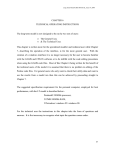
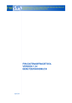
probability distributions of the parameters may be represented on an event tree, such as the
one of figure 1, depicting a typical energy/environmental situation. In figure 1, two
parameters are uncertain: mitigation level, and demand growth rate. The first may have only
two values (High and Low), and becomes known in 2005. The second also may have two
values (High and Low) and becomes known in 2010. The probabilities of the outcomes are
shown along the branches. This example assumes that present time is 1995. This example is
said to have three stages (i.e. two resolution times). The simplest non-trivial event tree has
only two stages (a single resolution time).
High Growth 0.4
High Mitigation 0.5
Low Mitigation
0.6
0.5
0.5
Low Growth
Stage 1
1995
2000
Low Growth
High Growth
0.5
Stage 2
2005
2010
Stage 3
2015
2020
2025
2030
Figure 1. Event Tree for a three-stage stochastic TIMES Example.
2035
While stochastic programming is an advanced way to take into account uncertainties, a more
common and very useful way to analyze the impact of uncertainties is sensitivity analysis.
In sensitivity analysis, the values of some important exogenous assumptions are varied, and
a series of model runs is performed over a discrete set of combinations of these assumptions.
Sensitivity analysis is often combined with tradeoff analysis, where the tradeoff relation
between several objectives is analyzed. The stochastic mode provides an efficient tool for
both sensitivity and tradeoff analyses, because it enables the use of so-called uncertain attributes. The uncertain attributes are similar to the corresponding standard TIMES attributes,
but they can be defined over a discrete set of states-of-the-world (SOW). In stochastic programming the SOWs correspond to the branches of the event tree, but they can equally well
be used for sensitivity analysis, so that the model is sequentially run over the set of SOWs,
using the corresponding values of the uncertain attributes in each individual run.
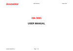
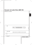
Figure 2 illustrates a few possible set-ups for sensitivity and tradeoff analyses in TIMES, all
of which are supported by the model generator:
A. Simple sensitivity analysis over the set of SOWs.
B. Two-phase tradeoff analysis, where the model is first run once using a user-defined
objective function, and then the solution from the first phase is used for defining
additional constraints in a series of model runs in the second phase.
C. Two-phase tradeoff analysis, where the model is first run over a set of SOWs, each
of which may have a different objective functions and different parameter attributes.
In Phase 2 the solution for each SOW from Phase 1 is used for defining additional
constraints for each SOW in Phase 2, where the standard objective function is used.
D. Two-phase tradeoff analysis, where the model is first run over a set of SOWs, each
of which have a different objective function and optionally different UC RHS. In
Phase 2 the solution for each SOW obtained from Phase 1 is used for defining an
additional deviation constraint for each of the objectives used in Phase 1, and a
single model is solved in Phase 2 optimizing the standard objective function.
E. Multiphase tradeoff analysis over N phases with different objective functions.
Sensitivity
analysis
(A)
Multiphase
analysis
Two-phase tradeoff analysis
(B)
1
1
2
(C)
(D)
2
1
2
1
1
1
1
1
2
2
2
2
1
2
(E)
1
2
1
3
3
3
3
3
3
N
N
N
N
N
N
Figure 2. Possible set-ups for sensitivity / tradeoff analysis.
2. MULTI-STAGE STOCHASTIC PROGRAMMING
2.1 General
The key observation is that prior to resolution time, the decision maker (and hence the
model) does not know the eventual values of the random parameters, but still has to take
decisions. On the contrary, after resolution, the decision maker knows with certainty the
outcome of some event(s) and his decisions will be different depending of which outcome
has occurred.
For the example of figure 1, in 2000 and 2005 there can be only one set of decisions,
whereas in 2010 there will be two sets of decisions, contingent on which of the Mitigation
outcomes (High or Low) has occurred, and in 2015, 2020, ..., 2035, there will be four sets of
contingent decisions.
This remark leads directly to the following general multi-period, multi-stage stochastic
program (1) –(3) below. The formulation described here is based on Dantzig (1955), Wets
(1989), or Kanudia and Loulou (1998), and uses the expected cost criterion. Note that this is
a LP, but its size is larger than that of the deterministic TIMES model.
Minimize
Z=∑
∑
C(t,s) × X(t, s) × p(t, s)
(1)
A(t , s) × X (t , s) ≥ b(t, s )
∑ D(t , g (t , s)) × X (t , g (t , s)) ≥ e( s)
(2)
(3)
t∈T s∈S(t)
Subject to:
∀s ∈ S (T )
t∈T
where
t
T
s
S(t)
=
=
=
=
S(T)
=
g(t,s) =
X(t,s) =
C(t,s) =
time period
set of time periods
state index
set of state indices for time period t; for Figure 1, we have:
S(1995) = 1; S(2000) = 1; S(2005) = 1; S(2010) = 1,2; S(2015) = 1,2,3,4;
S(2020) = 1,2,3,4; S(2025) = 1,2,3,4; S(2030) = 1,2,3,4; S(2035) = 1,2,3,4;
set of state indices at the last stage (the set of scenarios). Set S(T) is
homeomorphic to the set of paths from period 1 to last period, in the event
tree.
a unique mapping from {(t , s) | s ∈ S (T )} to S(t), according to the event tree.
g(t,s) is the state at period t corresponding to scenario s.
the column vector of decision variables in period t, under state s
the cost row vector
p(t,s) =
A(t,s) =
b(t,s) =
D(t,s) =
e(s) =
event probabilities
the LP sub-matrix of single period constraints, in time period t, under state s
the right hand side column vector (single period constraints) in time period t,
under state s
the LP sub-matrix of multi-period constraints under state s
the right hand side column vector (multi-period constraints) under
scenario s
Alternate formulation: The above formulation makes it a somewhat difficult to retrieve
the strategies attached to the various scenarios. Moreover, the actual writing of the
cumulative constraints (3) is a bit delicate. An alternate (but equivalent) formulation
consists in defining one scenario per path from initial to terminal period, and to define
distinct variables X(t,s) for each scenario and each time period. For instance, in this
alternate formulation of the example, there would be four variables X(t,s) at every
period t, (whereas there was only one variable X(1995,1) in the previous formulation).
Minimize
Z=∑
∑ C(t, s) × X(t, s) × p(t, s)
(1')
t∈T s∈S(t)
Subject to:
A(t , s) × X (t , s) ≥ b (t, s )
all t, all s
(2')
∑ D(t , s) × X (t , s) ≥ e(s)
all t, all s
(3')
t∈T
Of course, in this approach we need to add equality constraints to express the fact that
some scenarios are identical at some periods. In the example of Figure 1, we would have:
X(1995,1)=X(1995,2)=X(1995,3)=X(1995,4),
X(2000,1)=X(2000,2)=X(2000,3)=X(2000,4),
X(2005,1)=X(2005,2)=X(2005,3)=X(2005,4),
X(2010,1)=X(2010,2),
X(2010,3)=X(2010,4).
Although this formulation is less parsimonious in terms of additional variables and
constraints, many of these extra variables and constraints are in fact eliminated by the
pre-processor of most optimizers. The main advantage of this new formulation is the ease
of producing outputs organized by scenario.
In the current implementation of stochastic TIMES, the first approach has been used
(Equations 1-3). The results are however reported for all scenarios in the same way as in
the second approach.
2.2 Alternative objective formulations
The preceding description of stochastic programming assumes that the policy maker
accepts the expected cost as his optimizing criterion. This is equivalent to saying that he
is risk neutral. In many situations, the assumption of risk neutrality is only an approximation of the true utility function of a decision maker.
Two alternative candidates for the objective function are:
•
•
Expected utility criterion with linearized risk aversion
Minimax Regret (Savage) criterion (Loulou and Kanudia, 19991)
Expected Utility Criterion with risk aversion
The first alternative has been implemented into the stochastic version of TIMES. This
provides a feature for taking into account that a decision maker may be risk averse, by
defining a new utility function to replace the expected cost.
The approach is based on the classical E-V model (an abbreviation for Expected ValueVariance). In the E-V approach, it is assumed that the variance of the cost is an
acceptable measure of the risk attached to a strategy in the presence of uncertainty. The
variance of the cost of a given strategy k is computed as follows:
Var (Ck ) =
∑p
j
• (Cost j k − ECk )2
j
where Costj|k is the cost when strategy k is followed and the jth state of nature prevails,
and EC k is the expected cost of strategy k, defined as usual by:
EC k =
∑p
j
• Cost j k
j
An E-V approach would thus replace the expected cost criterion by the following utility
function to minimize:
U = EC + λ ⋅ Var (C )
where >0 is a measure of the risk aversion of the decision maker. For =0, the usual
expected cost criterion is obtained. Larger values of indicate increasing risk aversion.
For =0, one gets the simple expected cost criterion.
1
Loulou, R., and A. Kanudia (1999) “Minimax Regret Strategies for Greenhouse Gas Abatement: Methodology
and Application”, Operations Research Letters, 25, 219-230.
Taking risk aversion into account by this formulation would lead to a non-linear, nonconvex model, with all its ensuing computational restrictions. These would impose
serious limitations on model size.
Utility Function with Linearized Risk Aversion
To avoid non-linearities, it is possible to replace the semi-variance by the Upperabsolute-deviation, defined by:
{
UpAbsDev(Costk ) = ∑ p j • Costj k − ECk
}
+
j
+
where y= {x} is defined by the following two linear constraints: y
the utility is now written via the following linear expression:
x , and y
0, and
U = EC + λ ⋅ UpsAbsDev(C )
This is the expected utility formulation implemented into the TIMES model generator.
Note that this linearized version of the risk averse utility function is not available in the
MARKAL code.
2.3 Solving approaches
General multi-stage stochastic programming problems of the type described above can be
solved by standard deterministic algorithms by solving the deterministic equivalent of the
stochastic model. This is the most straightforward approach, which may be applied to all
problem instances. However, the resulting deterministic problem may become very large
and thus difficult to solve, especially if integer variables are introduced, but also in the
case of linear models with a large number of stochastic scenarios.
Two-stage stochastic programming problems can also be solved efficiently by using a
Benders decomposition algorithm (Kalvelagen, 2003). Therefore, the classical decomposition approach to solving large multi-stage stochastic linear programs has been nested
Benders decomposition. However, a multi-stage stochastic program with integer variables does not, in general, allow a nested Benders decomposition. Consequently, more
complex decompositions approaches are needed in the general case (e.g. Dantzig-Wolfe
decomposition with dynamic column generation, or stochastic decomposition methods).
The current version of the TIMES implementation for stochastic programming is solely
based on directly solving the equivalent deterministic problem. As this may lead to very
large problem instances, stochastic TIMES models are in practice limited to a relatively
small number of scenarios.
3. TRADEOFF ANALYSIS
Analyzing tradeoffs between the standard objective function and some other possible
objectives (for which the market is not able to give a price) has not been possible in an
effective way until TIMES version 2.5.0. The tradeoff analysis facility is available under
the stochastic mode of TIMES, which provides the basic tool for making sensitivity
analyses over a number of different cases. In addition to providing the means for
specifying the parameters to be varied in the sensitivity analysis, the tradeoff facility
provides a tool for making a two-phase or a multiphase tradeoff analysis using a
completely user-defined objective functions in the first phase, or even in several phases.
3.1 Two-phase tradeoff analysis
In the first phase of the TIMES two-phase tradeoff analysis facility, the objective
function can be defined as a weighted sum of any number of objective components. All
of the components will refer to the LHS value of a global user constraint (i.e. a user
constraint that is summed over regions and periods). Each of the component UCs can be
either fully non-constraining or constrained by upper/lower bounds on the LHS. The
components are defined by the user by specifying non-zero weight coefficients for the
UCs to be included in the objective. The original objective function (total discounted
costs) is automatically pre-defined as a non-constraining user constraint with the name
‘OBJZ’, and can therefore always be directly used as one of the component UCs, if
desired.
Consequently, the first phase can be considered as representing a simple Utility Tradeoff
Model, which can also be used as a stand-alone option. The resulting objective function
to be minimized can be written as follows:
min obj1 =
∑W (uc) • LHS (uc)
uc∈UC _ GLB
where:
W(uc)
LHS(uc)
UC_GLB
=
=
=
weight of objective component uc in Phase 1
LHS expression of user constraint uc according to its definition
the set of all global UC constraints (including ‘OBJZ’)
In the second phase of the TIMES two-phase tradeoff analysis facility the objective
function is always the original objective function in TIMES, i.e. the total discounted
system costs.
In addition, in the second phase the user can specify bounds on the proportional deviation
in the LHS value of any user constraint, in comparison to the optimal LHS value
obtained in the first phase. Such deviation bounds can be set for both global and nonglobal constraints, and for both non-constraining and constrained UCs (any original
absolute bounds are overridden by the deviation bounds). The objective function used in
Phase 1 is now available as an additional pre-defined UC, named ‘OBJ1’, so that one can
set either deviation bounds or absolute bounds on that as well, if desired. In addition, both
the total and regional original objective function can be referred to by using the predefined UC name ‘OBJZ’in the deviation bound parameters.
The objective function to be minimized in the second phase, and the additional bounds on
the LHS values of UCs, can be written as follows:
min objz =
LHS (' OBJZ ' )
for each uc for which
LHS (uc) ≤ (1 + maxdev(uc)) • LHS * (uc) 

*
LHS (uc) ≥ (1 − maxdev(uc)) • LHS (uc)  maxdev(uc) has been specified
where:
LHS(‘OBJZ’)
LHS(uc)
LHS*(uc)
maxdev(uc)
=
=
=
=
the standard objective function (discounted total system costs)
LHS expression of user constraint uc according to its definition
optimal LHS value of user constraint uc in Phase 1
user-specified fraction defining the max. proportional deviation in
the value of LHS(uc) compared to the solution in Phase 1
Remarks:
1. Use of the two-phase tradeoff analysis facility requires that a weight has been
defined for at least one objective component in the first phase.
2. If no deviation bounds are specified, the second phase will be omitted.
3. Automatic discounting of any commodity or flow-based UC components is
possible by using a new UC_ATTR option ‘PERDISC’(see Section 4.4), which
could be applied e.g. to the user-defined objective components in Phase 1.
4. The two-phase tradeoff analysis can be carried over a set of distinct cases, each
identified by a unique SOW index.
3.2 Multiphase tradeoff analysis
The multiphase tradeoff analysis is otherwise similar to the two-phase analysis, but in this
case the objective function can be defined in the same way as in the Phase 1 described
above also in all subsequent phases. The different objective functions in each phase are
distinguished by using an additional phase index (the SOW index). Deviation bounds can
be specified in each phase, such that they will be in force over all subsequent phases (any
user constraints), or only in some of the succeeding phases (any user constraints
excluding OBJ1). The deviation bounds defined on any of the user-defined objectives
OBJ1 will thus always be preserved over all subsequent phases.
Remark:
1. Although the multiphase tradeoff analysis allows the use of any user-defined
objective functions in each phase, it is highly recommended that the original
objective function be used in the last phase, so that the economic sense is
maintained in the final solution.
4. GAMS IMPLEMENTATION
4.1 Overview
The handling of multi-stage stochastic programming has been implemented into the
GAMS code of the TIMES model generator. The stochastic mode is activated by the
following setting in the run file:
$ SET STAGES
YES
All the required control and input data parameters must also be specified, as explained in
the following sections. The stochastic results can be made available to the VEDA-BE
report generator as explained in Section 5.6.
4.2 Stages, states of the world and scenarios
The predefined set J constitutes the domain of the stochastic stages. The members of this
predefined set are named '1', '2', '3', ...'50'. Therefore, in principle, a maximum of 50
stages could be defined in the event tree. The actual number of stages in a model will be
one larger than the sequence number of the last stage for which the number of sub-states
SW_SUBS is specified (see below).
The predefined set ALLSOW constitutes the domain of possible states of the world.
Currently it has been defined to include the members '1', '2', '3', ...'64'. In other words, the
maximum number of states of the world is 64. Consequently, a binary event tree could
include at most 7 stages, because 2^6=64. In each stage of the event tree, the states of the
world are identified by sequential integers starting from 1. For example, if there are three
states in the second stage, these are identified by the numbers 1, 2 and 3. If all these three
states have two sub-states in the third stage, those will be numbered 1,2, ..., 6, so that the
states 1 and 2 in the third stage are sub-states of state 1 in the second stage. The states of
the world defined for the final stage of the event tree constitute the actual set of different
final states to be handled, also called scenarios. The set of final states, SOW, is then of
course also a subset of the domain ALLSOW. The alias name W is defined for SOW and
the name WW is defined for ALLSOW.
Internally, the states of the world are numbered differently in the intermediate stages. The
internal numbering is obtained by enumerating all stages p, excluding the last stage, in
reverse order. If the first sub-state of a certain state in stage p is k in stage p+1, this state
will be internally numbered k in stage p, instead of the sequential number. However,
actually the user does not need to know anything about this internal numbering, as all the
input parameters will use the original numbering based on sequential numbers at each
stage. The results, on the other hand, are for all periods reported for all of the states at the
final stage, because the states at the final stage represent the unique scenarios across the
periods. The mapping of the scenario indexes to the original state indexes in each period
is left to the user.
4.3 Parameters for stochastic programming
4.3.1
User control parameters
All control parameters for stochastic programming are available in the VEDA-FE shell,
where they may be specified by the user. All control parameter have a prefix 'SW_' in the
GAMS code of the model generator. The parameters are discussed in more detail below:
1. The parameter SW_START is used to indicate when each of the stochastic stages
begins. For stage 1, the value SW_START is always assumed to be the first
MILESTONYR. If any SW_START for subsequent stages is not equal to one of
the milestone years, it will be replaced by the first MILESTONYR following it. If
SW_START is not specified for some stage > 1, the MILESTONYR following the
SW_START of the previous stage is assumed. In addition, stages can also be
combined, see section 3.3.2.
2. The parameter SW_SUBS specifies the number of sub-states of the world for each
SOW at stage j. If it is not specified for stage 1, the number is determined by
using the following two rules:
•
If SW_SUBS or SW_SPROB is specified for any SOW at any stage, the largest
ordinal number of the SOWs in stage 2 for which either SW_SUBS or
SW_SPROB is specified is used, or 1 if none is specified at stage 2.
•
If neither SW_SUBS nor SW_SPROB is specified for any stage, the largest
ordinal number of the SOWs for which SW_PROB is specified is used.
3. The parameter SW_SPROB can be used to specify the conditional probabilities of
the sub-states of the world of each SOW at each stage j. Another way to specify
the probabilities is to specify the total probabilities of each SOW (at the last
stage), see SW_PROB.
Table 1. Control parameters for Stochastic TIMES.
Parameter
SW_START(j)
SW_SUBS(j, w)
SW_SPROB(j, w)
SW_PROB(w)
SW_LAMBDA
Description
The year corresponding to the resolution of uncertainty at each
stage, and thus the last year of the hedging phase and the point
from which the event tree fans out for each of the SOW.
The number of sub-states of the world for each SOW at stage j.
The conditional probability of each sub-state at stage j. These
conditional probabilities can be overridden by SW_PROB.
The total probability of each SOW at the last stage. If specified,
overrides the stage-specific conditional probabilities.
Risk aversion coefficient.
4. The parameter SW_PROB can be used to specify the total probability of each
SOW (at the last stage). If specified, the total probability will override the total
probability derived from the stage-wise conditional probabilities. Another way to
specify the probabilities is thus to specify the conditional probabilities for the substates of the world at each stage. If the resulting final total probabilities will not
sum up to 1, they will be simply normalized over all SOWs.
5. The parameter SW_LAMBDA can be used to specify the risk aversion coefficient.
If not specified, the objective function represents the expected total discounted
system costs without risk aversion.'
4.3.2
Combining stages
Stages of the event tree can also be combined, if deemed useful. Any successive stages
will be combined into a single stage if the starting year of the succeeding stage is less
than or equal to the preceding stage. For example, if in the example of Figure 1 the
starting year of both stages 2 and 3 would be specified to be 2010, the stages 2 and 3
would be combined so that in 2010 the event tree is expanded directly from one state of
the world to four states. By using this feature, stages can even be combined with the first
stage, by specifying the same value of SW_START for both stage 1 and some subsequent
stages. If all stages were combined with the first stage, the resulting model would
optimize all the scenarios independently of each other. This feature can be used for
making a deterministic run for each scenario. This can be done best by specifying a large
value of SW_START for the first stage, and by leaving the other values intact.
Combined stages can be also useful for data management, for example, when the states at
stage 2 should contain some combinations of uncertain parameters. In such cases it can
be useful to define the scenarios for the uncertain parameters at successive stages so that
cloning becomes possible. Then the combined scenarios for stage 2 can be formed by
combining these successive stages.
4.3.3
Cloning parts of the event tree
If there are more than 2 stages in the event tree, the user can optionally utilize a cloning
facility for both the specification of the event tree and the specification of uncertain
parameters. At each stage, cloning can be used for those SOWs, for which the number of
sub-states of the world is equal to the number of sub-states for the first SOW. Cloning can
in this case be activated by leaving the number of sub-states unspecified for the SOWs to
be cloned. The model generator will then assume the same number of sub-states as for
the first SOW. For such cloned nodes of the event tree, both the conditional probabilities
and the uncertain parameters of the sub-states will be copied from the sub-states of the
first SOW, whenever they have not been specified by the user. The user can thus always
override the cloning by simply specifying the probabilities and/or uncertain parameters
explicitly.
Cloning of the event tree can be convenient if the event tree is large, because then it can
considerably reduce the amount of input data needed.
4.3.4
Uncertain input parameters
In this first version of the stochastic TIMES, the only a few uncertain input parameters
have been implemented, as shown in Table 2. At a later stage more uncertain parameters
may of course be added. All the uncertain input parameters have a prefix 'S_'. The
uncertain parameters can be divided into two types: absolute and relative:
Absolute parameters are applied in the same way as their deterministic counterparts,
and they override the corresponding deterministic parameters in the parts of the event tree
where they apply. Absolute parameters defined at a later stage of the event tree also override those defined at an earlier stage. All uncertain bound attributes are of absolute type.
Relative parameters are applied as multipliers to the corresponding deterministic baseline parameters. Relative parameters are also applied cumulatively over stages, so that
any relative parameters defined at an earlier stage of the event tree are included in the
combined multipliers at a later stage. Consequently, for any branches downstream in the
event tree the current branch represents the baseline for which the multipliers in the
succeeding stage will be applied. Uncertain demand projections have been implemented
in TIMES as relative parameters. This means that the uncertain demands are expressed as
multipliers applied to the baseline demand projection. The advantage of the relative
parameters is that, when appropriate, they are easier to maintain that absolute parameters.
The user can also utilize the cloning facility described above for the specification of the
uncertain parameters. As with the stage-wise conditional probabilities, cloning of
uncertain parameters is done at some stage j if all of the following three conditions hold:
•
•
•
The parameter has been specified for the sub-states of the first SOW at stage j;
The number of sub-states was left unspecified for some other SOW at stage j;
The uncertain parameter has not been specified for some of the sub-states of SOW,
which are thus considered subject to cloning.
Table 2. Current set of uncertain input parameters for stochastic TIMES.
Parameter
Description
S_COM_PROJ(r,y,c,j,w)
S_CAP_BND (r,y,p,l,j,w)
S_COM_CUMPRD(r,y,y,c,l,j,w)
S_COM_CUMNET(r,y,y,c,l,j,w)
S_FLO_CUM(r,p,c,y,y,l,j,w)
S_FLO_FUNC(r,y,p,cg1,cg2,j,w)
S_NCAP_COST(r,y,p,j,w)
S_UC_RHSxxx(… ,l,j,w)
S_DAM_COST(r,y,c,cur,j,w)
S_CM_MAXC (y,item,j,w)
S_CM_CONST(item,j,w)
Demand projection
Bound on total installed capacity
Cumulative bound on commodity production
Cumulative bound on commodity net prod.
Cumulative bound on flow or activity
Process transformation / efficiency
Process investment cost
RHS constant of user constraint
Damage cost of net production of commodity
Bound on maximum level of climate variable
Climate module constant (CS or SIGMA1)
Type
Rel.
Abs.
Abs.
Abs.
Abs.
Rel.
Rel.
Abs.
Abs.
Abs.
Abs.
The last two indexes of all uncertain parameters are j (stage) and w (state of world). The
stage index has been included in the parameters to ensure unambiguity; without the stage
index there could easily be ambiguities in the parameter values for earlier stages. Note
that demand projections are by default interpolated and extrapolated over all valid periods
for each stage. Bound parameters are by default interpolated within periods only.
Example:
The event tree of the example shown in Figure 1 can be specified as follows:
PARAMETER SW_START
PARAMETER SW_SUBS
PARAMETER SW_SPROB
/ 2 2010 /;
/ 2.1 2, 2.2 2/;
/ 2.1 0.5, 3.1 0.4, 3.3 0.5/;
Assume that High Mitigation in Figure 1 corresponds to a constant CO2 concentration
limit of 770 between 2010 and 2035, and Low Mitigation corresponds to the limits of 790
and 950 in 2010 and 2035, respectively. The mitigation parameters can then be specified
as follows (the year index 0 is a placeholder for the interpolation control option):
PARAMETER S_CM_MAXCO2C / 0.2.1 1, 2010.2.1 770, 2035.2.1 770
0.2.2 1, 2010.2.2 790, 2035.2.2 950/;
Assume that High Growth is 5% higher than the baseline projection, and Low Growth is
5% lower. The High/Low growth parameters can then be specified as follows (assuming
that the region is 'REG' and the demand is 'DEM':
PARAMETER S_COM_PROJ / REG.2015.DEM.3.1
REG.2015.DEM.3.2
REG.2015.DEM.3.3
REG.2015.DEM.3.4
1.05,
0.95,
1.05,
0.95 /;
Table 3. GAMS control variables for stochastic TIMES.
Control
variable
EQ
VAR
VART
VARM
VARV
SOW
SWD
SWTD
SWT
SWS
Value of control variable
Standard
"EQ"
"VAR"
"VAR"
"VAR"
"VAR"
""
""
""
""
""
Under stochastics
"ES"
"VAS"
"SUM(SW_TSW(SOW,T,W),VAS"
"SUM(SW_TSW(SOW,MODLYEAR,W),VAS"
"SUM(SW_TSW(SOW,V,W),VAS"
",SOW"
",WW"
",T,WW"
",SW_T(T,SOW)"
",W)"
Table 4. Internal sets and parameters for stochastic TIMES.
Set
Description
SW_ CHILD(j,w,w)
Child sub-states of the world for each SOW at each stage
SW_ COPY(j,w)
SOWs at each stage for which cloning is applied
SW_ MAP(t,w,j,w)
Mapping from period and internal SOW to stage and original SOW
SW_ STAGE(j,w)
Internal SOWs at each stage
SW_ T(t,w)
Valid internal SOWs in each period
SW_ TOS(w,t,w)
Mapping from redundant scenarios to unique SOW in each period t
SW_TREE(j,w,w)
Scenarios for each original SOW at each stage
SW_ TSTG(t,j)
Valid stages j for each period t
SW_ TSW(w,t,w)
Mapping from all scenarios to unique SOW in each period t
SW_ UCT(uc_n,t,w)
Valid internal SOWs in each period for period-wise user constraints
Parameter
Description
SW_ DESC(j,w)
Number of scenarios for each original SOW at each stage
SW_ TPROB(t,w)
Probability of each internal SOW in each period
4.3.5
Internal sets, parameters and control variables
The implementation uses a few internal sets and parameters. All the internal sets and
parameters have a prefix 'SW_'. Table 4 gives an overview of these sets and parameters.
The implementation of the stochastic extension uses a number of GAMS control
variables for renaming and adjusting the equations and variables for the additional
dimension needed for stochastic programming. Table 3 summarizes the control variables.
4.3.6
Reporting parameters
All standard reporting parameters have a prefix 'S', and the first index is always the
stochastic scenario index. Reporting parameters for the Climate Module have a prefix
'CM_S'. The scenario index is always the first dimension of the parameters. The
stochastic reporting parameters provide almost the same set of results as those that have
been transferred to VEDA-BE from standard TIMES model runs, but now for each of the
stochastic scenarios. However, there are a few small differences:
•
•
All the undiscounted cost results from stochastic runs represent annualized costs,
and they are divided into genuine costs and taxes/subsidies. Decommissioning
costs are annualized over the same years as fixed costs.
The activity costs and flow costs are reported at the ANNUAL level only, while
in the standard reports they are reported in each timeslice.
•
•
Reporting parameters for the levels of commodity balance and peak equations
have been omitted from the stochastic reports, because the levels are normally
zero anyway (except for demands). Only the marginals are thus reported.
Under the stochastic mode, all user constraints are formulated by using slacks,
and therefore the reporting parameters for user constraints represent the levels and
marginals of these slack variables.
Table 5. Reporting parameters for stochastic TIMES.
Parameter
Description
Cost parameters
SREG_WOBJ(w,r,item,cur)
Discounted objective value by region, type and currency
SCST_INVC(w,r,v,t,p)
Annualized undiscounted investment costs
SCST_INVX(w,r,v,t,p)
Annualized undiscounted investm. taxes and subsidies
SCST_DECC(w,r,v,t,p)
Annualized undiscounted decommissioning costs
SCST_FIXC(w,r,v,t,p)
Undiscounted fixed costs
SCST_FIXX(w,r,v,t,p)
Undiscounted fixed taxes and subsidies
SCST_ACTC(w,r,v,t,p)
Undiscounted activity costs
SCST_FLOC(w,r,v,t,p,c)
Undiscounted flow costs
SCST_FLOX(w,r,v,t,p,c)
Undiscounted flow taxes and subsidies
SCST_COMC(w,r,t,c)
Undiscounted commodity costs
SCST_COMX(w,r,t,c)
Undiscounted commodity taxes and subsidies
Level parameters
SF_IN (w,r,v,t,p,c,s)
Flows into processes
SF_OUT (w,r,v,t,p,c,s)
Flows out of processes
SPAR_ACTL(w,r,v,t,p,s)
Activity levels of processes
SPAR_CAPL(w,r,t,p)
Total installed capacities of processes
SPAR_NCAPL(w,r,t,p)
Newly installed capacities of processes by period
SPAR_COMPRDL(w,r,t,c,s)
Commodity gross production levels
SPAR_COMNETL(w,r,t,c,s)
Commodity net production levels
SPAR_UCSL(w,uc,*,*,*)
Levels for the user constraint equations (slacks)
Marginal parameters
SPAR_ACTM(w,r,v,t,p,s)
Marginals for the activity variables
SPAR_CAPM(w,r,t,p)
Marginals for the total installed capacity variables
SPAR_NCAPM(w,r,t,p)
Marginals for the new capacity variables
SPAR_COMPRDM(w,r,t,c,s)
Marginals for the commodity production variables
SPAR_COMNETM(w,r,t,c,s)
Marginals for the commodity net variables
SPAR_COMBALEM(w,r,t,c,s)
Marginals for the commodity balance equations (=E=)
SPAR_COMBALGM(w,r,t,c,s) Marginals for the commodity balance equations (=G=)
Table 5. Reporting parameters for stochastic TIMES.
Parameter
Description
SPAR_PEAKM(w,r,t,cg,s)
Marginals for the peak equations
SPAR_UCSM(w,uc,*,*,*)
Marginals for the user constraint equations (slacks)
Capacity bound parameters
SPAR_CAPUP(w,r,t,p)
Upper bound on overall capacity in a period
SPAR_CAPLO(w,r,t,p)
Lower bound on overall capacity in a period
Climate module result parameters
CM_SRESULT(w,item,t)
Basic results from stochastic Climate Module
CM_SMAXC_M(w,y)
Shadow price of climate variable constraint
The reporting parameters for the Climate Module correspond to the same ones in the
standard mode, with the adjunction of the prefix CM_S.
4.4 Parameters for tradeoff analysis
The two-phase tradeoff analysis facility is available under the stochastic mode only. The
stochastic mode should therefore be activated, when using the tradeoff analysis facility. If
no SOWs are explicitly defined by the user, the model will be run only once (SOW=1)
using the two solution phases described above in Section 3. However, usually the user
would like to estimate a full tradeoff curve, consisting of a number of discrete solution
points (SOW=1,…,N). The number of points in the curve, i.e. the number of SOWs, should
be defined by SW_SUBS('1', '1') = N;
The parameter attributes that can be varied in such sensitivity analyses are the same
uncertain parameters, which can also be used for multi-stage stochastic programming.
The following uncertain attributes are perhaps the most important for tradeoff analyses:
•
•
Uncertain RHS constants of user constraints
Uncertain damage costs
Table 6. New input parameters for two-phase tradeoff analysis in TIMES.
Parameter
S_UCOBJ
(uc_n,w)
UC_ATTR
(r,uc_n,’
LHS’
,grp,’
PERDISC’
)
Description
Weight coefficients for the components of the objective
function in the first phase of the tradeoff facility, and for
each SOW to be analyzed (max. 64 different cases).
Interpolation: Not available.
Flag indicating that discounting is to be applied to the
periods in the LHS side of UC constraint. Applicable to
UC components (grp) UC_ACT, UC_FLO, UC_IRE,
UC_COMPRD, UC_COMNET and UC_COMCON, for
any UC summed over periods.
The weight parameter W, which defines the coefficients for the user-defined objective
components (see Section 3) can be specified by using the parameter S_UCOBJ, as
described in Table 6. Optional discounting of any flow-based UC components can be
activated by using the UC_ATTR option 'PERDISC'. The two-phase solution procedure
can be run over a maximum of 64 different cases (SOWs), each of which may have
different values for any of the uncertain parameters. The deviation bounds to be defined
in Phase 2 can be specified with the UC_RHSxxx attributes, by using the 'N' bound
type. Any non-negative 'N' value will be applied as a deviation bound in the second
phase. The bound value represents the maximum proportional deviation allowed in the
value of the LHS expression of the UC constraint, as described in Section 3. Negative
'N' bounds are ignored, and therefore negative bound values can always be safely used
for generating non-constraining user-defined equations for reporting purposes. By using
the uncertain S_UC_RHSxxx attributes, the deviation bounds to be applied in Phase 2
can be varied over SOWs. The predefined UC names 'OBJZ' and 'OBJ1' can be used in
deviation bounds to refer to the original or user-defined objective functions, respectively
('OBJZ' also by region). 'OBJZ' can naturally also be used also in S_UCOBJ.
Remark: If the objective in Phase 1 is defined for only a single SOW (1), the same objective will also be used for any subsequent SOW points to be analyzed (according to the
number of SOW as defined by SW_SUBS('1', '1')).
4.5 Stochastic variables
As noted earlier, the variables that are used to model the stochastic programming version
of TIMES are the same variables that make up the deterministic TIMES model, with two
minor adjustments. The main difference is that the variables require another index
corresponding to the state-of-the-world, SOW. To standardize the handling of this index it
is always introduced after the period index, thus it is usually the second index (or the first
if there is no period index) in the variable. To accommodate this requirement each
standard model variable name is adjusted by replacing the standard prefix of the variable
name, VAR_, by VAS_. So for example the capacity variable, VAR_CAP(r,t,p) becomes
VAS_CAP(r,t,p,sow). During matrix generation the appropriate SOW index value is then
entered into VAS_CAP according to the set SW_T and the period being worked on.
Table 7. Variables for stochastic TIMES.
Variable
VAS_UC (‘
OBJZ’
,w)
VAS_UC (‘
OBJ1’
,w)
VAS_EXPOBJ
VAS_UPDEV (w)
Description
The variable equal to the sum of the total discounted system cost
associated with each SOW.
The variable equal to the total objective function in Phase 1 of the
Tradeoff Analysis facility (not used under multi-stage stochastics).
The variable equal to the expected value of the total discounted
system cost.
The upside deviation between the total system cost for each SOW
and the expected value of the total system cost.
As there is thus essentially no redefinition of the variables for the stochastic formulation,
other than the control of the instances of the variable according to the control sets SW_T
and SW_TSW, the user is referred to Chapter 4 of the TIMES Reference Manual for
details on the variables of the model. Below in Table 7 the variables strictly involved
with the stochastic version are listed, however as it is rather straightforward the
description of the variable details is not repeated here for the stochastic variables.
4.6 Equations
As noted earlier, and as is the case with the variables, the equations that are used to
model stochastics are the same equations that make up the non-stochastic TIMES model
with two minor adjustments. The main difference is that the equations require another
index corresponding to the state-of-the-world, SOW. To standardize the handling of this
index, either the SOW index as such or the set SW_T(t,sow) is introduced after all the
other indexes of the equation. The set SW_T is used instead of SOW whenever the
equation concerns a single period. To accommodate the required modifications, each
standard model equation name is adjusted by replacing the standard prefix in the equation
name, EQ_, by ES_. So, for example the capacity transfer equation, EQ_CPT(r,t,p)
becomes ES_CPT(r,t,p,SW_T(t,sow)). During matrix generation the appropriate SOW
index value is then entered into the ES_CPT equations according to the set SW_T and the
period being worked on.
As there is thus essentially no redefinition of the equations for the stochastic formulation,
other than the objective function (below) and the control over the generation of the
appropriate equations and variables according to the control sets SW_T and SW_TSW
mentioned above, the user is referred to Chapter 5 of the TIMES Reference Manual for
details on the core equations of the model. Below in Table 8 the few equations directly
related to only stochastic version are listed and briefly described. The equations include
the standard expected value for the stochastic objective function, the deviation equations,
and, finally, the formula for the generalized objective function including the risk aversion
Table 8. Equations for stochastic TIMES.
Equation
Description
ES_SOBJ (‘
N’
,w)
The total discounted cost associated with each SOW.
A) The expected value of the total discounted system cost, taking
into consideration the probability of each event path.
B) Under the two-phase Tradeoff Analysis, the user-defined
objective function in the first Phase.
The upside absolute deviation between the total system cost for
each SOW and the expected value of the total system cost.
These equations are generated only when the risk aversion
coefficient SW_LAMBDA has been specified.
The multi-objective function, i.e. the full objective function
whether risk is accounted for or not, by adding to the expected
cost a risk term obtained by multiplying the risk aversion intensity
SW_LAMBDA by the upside absolute deviation (probability
weighted sum of the upside deviations for every state of world).
ES_EXPOBJ
ES_UPDEV(w)
EQ_OBJ
penalties.
Note that the equation for the final objective function, EQ_OBJ, has the same name as in
standard TIMES, only the definition of this equation is different under the stochastic
mode. Similarly, also the objective variable ObjZ has the same name as in standard
TIMES.
4.7 Supported TIMES extensions
The implementation of stochastic programming has been extended to support the use of
multi-stage stochastic programming also with the following TIMES extensions that are
included in the standard distribution:
•
•
•
•
•
•
The Climate Module (CLI)
The Lumpy Investment extension (DSC)
The Endogenous Technological Learning extension (ETL)
The Damage Cost Functions (DAM)
The TIMES-VEDA-FE extension (VDA)
The IER extension of University of Stuttgart (IER)
The stochastic mode cannot be used with the new TIMES-MACRO model variant.
4.8 Changes in model generator code
The implementation required extensive modifications to the existing code as well as a
number of new components in the model generator. In total about 90 existing files were
modified, and 11 new code files were added.
The new code components are listed in Table 9. The new files that are solely related to
stochastic TIMES have the extension '.stc', with the exception of RPT_STC.cli, which is
the report driver for the Climate Module under stochastic programming. A new generalTable 9. New files in the TIMES model generator code.
File
Description
INITMTY.stc
STAGES.stc
RPTMAIN.stc
FILLSOW.stc
RENAME.stc
SOLVE.stc
COST_ANN.rpt
EQDECLR.mod
CAL_VAR.mod
RPT_PAR.cli
RPT_STC.cli
Declarations for the stochastic extension
Preprocessing and management of stochastic stages
Main driver for reporting results from stochastic runs
Cloning and processing of uncertain input parameters
Reporting of stochastic results in scenario files (used for ETL only)
Solving stochastic model with possible direct decomposition
Calculation of annual costs for stochastic results
Declaration of model equations (parametrization for stochastics)
Helper for inclusion of stochastic variables in inter-period equations
Calculation of the reporting parameters in the Climate Module
Driver for reporting of stochastic runs in the Climate Module
purpose routine for annual costs was implemented, and it is used for generating the
reporting cost parameters under stochastics (COST_ANN.rpt). To assist future changes
in the code, a small helper routine was implemented for the inclusion of generalized
variables in model equations (CAL_VAR.mod). This helper routine automates the
parametrization of the variables so that they will be correctly dimensioned and mapped, if
the model is run under stochastics.
The TIMES code files that were most substantially changed during the implementation
are listed in Table 10. All files that involve dynamic equations are here classified to have
undergone substantial changes, because dynamic equations require special handling of
the stochastic variables.
In addition, the file EQMAIN.mod was divided into two parts during the implementation
(EQDECLR.mod and EQMAIN.mod). Moreover, some files related to the ETL extension
were renamed to conform to the standard conventions for TIMES extensions.
Table 10. Code files of the TIMES model generator with substantial changes.
File
Description
BND_SET.mod
BNDMAIN.mod
CAL_CAP.mod
CAL_NCOM.mod
EQCAPACT.mod
EQCOMBAL.mod
EQCPT.mod
EQCUMCOM.mod
EQDAMAGE.mod
EQMAIN.mod
EQOBJ.mod
EQOBJELS.mod
EQOBJFIX.mod
EQOBJINV.mod
EQOBJVAR.mod
EQOBSALV.mod
EQPEAK.mod
EQSTGIPS.mod
EQUSERCO.mod
MAINDRV.mod
MOD_EQUA.mod
RPTMAIN.mod
ATLEARN.etl
EQU_EXT.etl
EQCAFLAC.vda
EQU_EXT.cli
RPT_EXT.cli
Uncertain bound parameters for capacities
Handling of stochastic indexes for bounds
Dynamic equations for capacity related flows
Dynamic equations for investment and decommissioning flows
Dynamic capacity utilization equations
Uncertain demand parameters
Dynamic capacity transfer equations
Dynamic cumulative commodity equations
Dynamic equations for objective component of damages
Handling of basic equation differences under stochastic TIMES
Objective functions for stochastic programming
Dynamic equations for objective component
Dynamic equations for objective component
Dynamic equations for objective component
Dynamic equations for objective component
Dynamic equations for objective component
Dynamic capacity/peaking equations
Dynamic storage equations
Dynamic and cumulative user constraints
Handling of the main control variables for stochastic TIMES
Parametrized equation declarations
Handling of report generation under stochastic TIMES
Reports from the ETL extension under stochastic TIMES
Dynamic learning equations (former EQUETL.etl)
Dynamic capacity utilization equations
Dynamic carbon balance equations, dynamic concentration bounds
Handling of report generation under stochastic TIMES
5. USER'S REFERENCE
5.1 Activating the stochastic mode
The stochastic mode can be activated by using the following setting in the run file:
$
SET STAGES YES
If the stochastic mode is used for sensitivity analysis only, it can be alternatively activated also by using the following setting:
$
SET SENSIS YES
All the control and input parameters of the stochastic extension are only available when
using either of these settings. When using the SENSIS setting for sensitivity analysis, the
model will be solved sequentially in each of the stochastic scenarios, using the basis
information from each run as a starting basis for the next run.
5.2 Specification of states of the world and scenarios
The user does not need to specify the stages, states of the world or scenarios explicitly.
The predefined domain for the stages is the set J, which contains the elements
'1','2',...,'50'. This should be sufficient for any conceivable stochastic TIMES model. The
predefined domain for the states is the set ALLSOW, which contains the elements
'1','2',...,'64'. Consequently, a maximum of 64 states (at any given stage) can be used in
the specification of a stochastic model. The same maximum amount applies, of course,
also to the scenarios, which are the states of the last stage.
5.3 Specification of input parameters
5.3.1
Specification of control parameters
1. Use the parameter SW_START to indicate when each of the stochastic stages
begins. SW_START is optional. The following rules apply:
•
•
•
•
For stage 1 no value needs to be specified (unless some stages are combined
into the first stage), because the first stage always starts in the first period.
If any SW_START specified for subsequent stages is not equal to one of the
milestone years, it will be automatically replaced by the first milestone year
following it.
If SW_START is not specified for some stage, the milestone year following
the SW_START of the previous stage is assumed.
Stages can be combined by specifying equal or decreasing values of
SW_START for successive stages.
•
Equivalent deterministic runs for each scenario can be made by specifying for
the first stage a value of SW_START larger than any milestone year.
2. Use the parameter SW_SUBS to specify the number of sub-states of the world for
each SOW at each stage j, if any. The use of SW_SUBS is required if more than
two stochastic stages are modeled. The following rules apply:
•
•
If SW_SUBS is not specified for stage 1, the number of states in stage 2 is
determined by the model generator from the other control parameters (for
details see section 4.3.1).
For any subsequent stages that have sub-states, SW_SUBS must be specified
for at least the first SOW. For those SOW that SW_SUBS is left unspecified,
the number of the first SOW is assumed, and these SOWs will be subject to
cloning.
3. Use the parameter SW_SPROB to specify the conditional probabilities of the substates of each SOW at each stage j. Alternatively, the total probabilities of each
SOW (at the last stage) can be specified, by using SW_PROB. The use of
SW_SPROB is the recommended method, for which the following rules apply:
•
•
If the parent SOW is subject to cloning, SW_SPROB can be left unspecified,
and it will then inherit the probabilities from the sub-states of the first SOW at
the previous stage.
If SW_SPROB is not specified and the parent SOW is not subject to cloning,
SW_SPROB will be automatically assigned a probability UP/m, where UP is
the unassigned probability among the sub-states of the parent SOW, and m is
the number of remaining sub-states for which probabilities are to be assigned.
An even probability distribution among the sub-states can thus be specified
without using any SW_SPROB (for non-cloned SOW), or by specifying the
probability for the first sub-state only (for cloned SOW).
4. Use the parameter SW_LAMBDA to specify the risk aversion coefficient. If not
specified, the objective function represents the expected total discounted system
costs without risk aversion.
A quick reference of the use of the control parameters is given in Appendix A.
5.3.2
Specification of uncertain parameters
The uncertain parameters shown in Table 11 can be currently used in stochastic TIMES.
A quick reference of the use of the input parameters is given in Appendix B. Apart from
the special aspects concerning the relative type, the use of the uncertain parameters is
basically similar to the corresponding deterministic parameters. However, the index of
both the stage and state of the world has to be specified when using these parameters. The
same default interpolation rules are applied to the uncertain parameters as to the
deterministic counterparts. Relative parameters are applied as multipliers to the corresponding deterministic baseline parameters, and cumulatively over stages. Any relative
parameters defined at an earlier stage of the event tree are included in the combined
multipliers at a later stage.
The user can also utilize the cloning facility for the automatic copying of uncertain
parameters from the sub-states of the first state at each stage to the sub-states of other
states. As mentioned above, these other states are subject to cloning only if SW_SUBS
was left unspecified for them.
5.4 Sensitivity analyses
The stochastic mode can also be used for a series of deterministic runs. This can be
accomplished by combining all (or some of) the stochastic stages with the first stage. An
easy way to do this is to specify for the first stage a value of SW_START larger than all
(or some of) the subsequent SW_START. Consequently, the subsequent stages will have a
value of SW_START less than or equal to the first stage, and are therefore combined with
the first stage. In effect, this will mean that all those branches of the event tree that are
distinct already at the first stage will be solved independently of each other. If all stages
are combined, the stochastic scenarios will be run fully independently. The SENSIS
setting described above will accomplish this without the need for setting SW_START.
Solving a set of deterministic scenarios in this way can be very useful for the following
different purposes:
•
For comparing the results from the stochastic model to the results of individual
deterministic scenarios;
•
For making standard sensitivity analysis with different values for the uncertain
parameters.
When the model generator detects that all scenarios are disjoint already at the first stage,
it uses the straightforward scenario decomposition approach to solving the problem.
Table 11. Initial set of uncertain input parameters for stochastic TIMES.
Parameter
Description
Type
S_COM_PROJ(r,y,c,j,w)
Demand projection
Rel.
S_CAP_BND (r,y,p,l,j,w)
Bound on total installed capacity
Abs.
S_COM_CUMPRD(r,y,y,c,l,j,w)
Cumulative bound on commodity production
Abs.
S_COM_CUMNET(r,y,y,c,l,j,w)
S_FLO_CUM(r,p,c,y,y,l,j,w)
S_FLO_FUNC(r,y,p,cg1,cg2,j,w)
S_NCAP_COST(r,y,p,j,w)
S_UC_RHSxxx(… ,l,j,w)
S_DAM_COST(r,y,c,cur,j,w)
S_CM_MAXC(y,item,j,w)
S_CM_CONST(item,j,w)
Cumulative bound on commodity net prod.
Cumulative bound on flow or activity
Process transformation / efficiency
Process investment cost
RHS constant of user constraint
Damage cost of net production of commodity
Bound on maximum level of climate variable
Climate module constant (CS or SIGMA1)
Abs.
Abs.
Rel.
Rel.
Abs.
Abs.
Abs.
Abs.
Thus, each scenario is in this case solved separately, one after another. The results are
still reported in the same way as in a standard stochastic run.
5.5 Example: Five-stage stochastic model
In section 4.3.4 a simple example of specifying a stochastic model was already given. In
this section a somewhat larger and more complete example is given, which however uses
the same uncertain parameters as the earlier example.
In the run file, the stochastic mode should be activated as follows:
* Define the model as stochastic:
$ SET STAGES YES
The specification of the event tree consists of the definition of the starting years of the
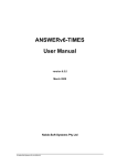
stages, the number of sub-states of each sow, and the probabilities. We are defining a
five-stage event tree, illustrated in Figure 3. In this example, we define the second stage
to start in 2010 and the third stage in 2020. We leave the start years of the fourth and fifth
stage unspecified, which means that they start in the milestone year succeeding the
previous stage (default definition).
PARAMETER SW_START
/ 2 2010, 3 2020 /;
We wish to have three states at the second stage, and all states will have two sub-states at
each subsequent stage. Here we can utilize the cloning facility, and therefore we need to
specify the number of sub-states for the first state at each stage only (and not for each
state of each stage).
PARAMETER SW_SUBS
/ 1.1 3, 2.1 2, 3.1 2, 4.1 2/;
If we wish to specify the conditional probabilities for the sub-states so that the distribution is the same under each parent state, we can use the cloning facility quite effectively for the specification of probabilities. For the second stage, we need to define the
probabilities for the first two states (the third is derived automatically). For the remaining
event tree, we only need to define the probability for the first state at each stage (the
second is derived):
PARAMETER SW_SPROB
/ 2.1 0.33, 2.2 0.34,
3.1 0.60, 4.1 0.55, 5.1 0.5 /;
However, if we wish to override the cloning of some probabilities, we can do that by
specifying the probabilities explicitly. Below, the probabilities of the sub-states of the last
branch at stage 4 are specified explicitly:
PARAMETER SW_SPROB
/ 4.12 0.7 /;
The uncertainty concerning climate change mitigation is assumed to be resolved at the
first stage. We assume a high, medium and low mitigation scenarios. In this example, we
assume that the high scenario corresponds to a CO2 concentration limit of 900 GtC in
2080, the medium scenario to 1150 and the low scenario to 1400 GtC in 2100,
respectively. For all scenarios, we assume that the limit evolves linearly from the value of
900 GtC in 2010. The mitigation parameters can then be specified as follows (the year
index 0 is a placeholder for the interpolation control option):
PARAMETER S_CM_MAXCO2C /0.2.1 1, 2010.2.1 900, 2080.2.1 900
0.2.2 1, 2010.2.2 900, 2080.2.2 1150
0.2.3 1, 2010.2.3 900, 2080.2.3 1400/;
The uncertainty concerning demand is assumed to be resolved gradually at the subsequent stages. At each stage we assume a high, and low growth scenario. At the third
stage, high growth is 7% higher and low growth is 4% lower than the baseline. At the
fourth stage high growth is 5% higher and low growth is 5% lower than the adjusted
baseline scenarios at previous stage. Finally, at the fifth stage high growth is 4% higher
and low growth is 7% lower than the adjusted baseline scenarios at the previous stage.
The cloning facility can again be effectively utilized for the demand data. Instead of
specifying the demand scenarios for all of the 42 nodes at the third, fourth and fifth stage,
we can specify the data for only six nodes corresponding to the sub-states of the first
nodes at the second, third and fourth stage. Note that the demand parameters are by
60%
33%
40%
60%
34%
40%
60%
33%
40%
Stage 1
Stage 2
2000
2010
Stage 3
2020
Stage 4
2030
2040
Stage 5
2050
2060
2070
Figure 3. Event Tree for a five-stage stochastic TIMES example.
2080
default interpolated and extrapolated over all valid periods for each stage, and thus only
one data point is needed. The demand scenarios can thus be fully specified as follows:
PARAMETER S_COM_PROJ / REG.2015.DEM.3.1
REG.2015.DEM.3.2
REG.2015.DEM.4.1
REG.2015.DEM.4.2
REG.2015.DEM.5.1
REG.2015.DEM.5.2
1.07,
0.96,
1.05,
0.95,
1.04,
0.93 /;
After running the stochastic model, the user might wish to compare the results with
equivalent deterministic scenarios. This can be accomplished by changing the start years
so that the first stage has a later start year than all other stages (see section 4.4):
PARAMETER SW_START / 1 9999, 2 2010, 3 2020 /;
5.6 Tradeoff analyses
5.6.1
Activating the tradeoff analysis mode
The tradeoff analysis facility has to be activated by either one of the following settings in
the run file:
$
$
SET STAGES YES
SET SENSIS YES
The first alternative simply activates the stochastic mode, which is required when using
the tradeoff facility. The second alternative additionally enables the use of the active
basis information successively between solving each point of the sensitivity analysis,
utilizing the so-called warm start method. In some cases, this may significantly improve
the solution speed, because the solution of each point can start from the optimal solution
of the previous point. However, in cases where the successive model instances to be
solved differ considerably from each other, this may not be an efficient option. The judgment of whether to use the warm start or not has to be made by the user. The set-ups D
and E described in the introduction are only possible with the setting STAGES YES.
When using the stochastic mode for tradeoff analysis, there is no need to specify any
other stochastic control parameters than the number of analysis points, which can be done
by specifying the number of SOW: SW_SUBS(‘1’,’1’) = N;
Therefore, the minimal specifications required to use the two-phase tradeoff analysis are
the following:
•
•
The stochastic mode is activated ($SET STAGES/SENSIS YES)
The weight parameter S_UCOBJ is defined for some UC and for either a single or
several SOW=1,… ,N (see Section 3 for syntax);
•
If the analysis is to be carried over several SOW, the user should additionally specify
the number N of the SOWs explicitly, by setting SW_SUBS(‘1’,’1’) = N; (default=1).
In addition, the user can define any of the uncertain parameters over the SOW to be
analyzed, and define deviation bounds by using either the deterministic or uncertain
UC_RHSxxx attributes, using the 'N' bound type and a non-negative bound value. The
predefined UC names 'OBJZ' and 'OBJ1' can be used in the RHS parameters to refer to
the original or user-defined objective functions, respectively ('OBJZ' also by region).
The set-up B described in the Introduction corresponds to the case where S_UCOBJ is
defined only for the first SOW. The corresponding set-ups D and E, which both have only
a single SOW in the final phase, can only be accomplished by activating the stochastic
mode by “$SET STAGES YES”, and by indicating the single terminal SOW by setting
S_UCOBJ('OBJ1','1'), where an explicit zero value (EPS) indicates that set-up D
is selected and any non-zero value indicates that set-up E is to be used. In addition, the
use of set-up D requires that no other uncertain parameters apart from S_UCOBJ and
S_UC_RHSxxx are specified, and deviation bounds can be specified only for OBJ1. In
the multiphase set-up E, all uncertain attributes can be freely used. However, in the
multiphase case the deviation bounds in each phase can be only be specified by using the
uncertain S_UC_RHSxxx parameters. The deviation bounds defined for each OBJ1 i are
in the multiphase case always preserved over all subsequent phases SOW = i+1,… ,N. Any
other deviation bounds defined for SOW = i are also preserved, unless explicitly canceled
in any subsequent phase SOW = k (k > i), by using the 'N' bound type, in which case the
bounds remain in force in phases SOW = i+1,… ,k.
5.6.2
Possible uses of the tradeoff facility
The simple facility described above can be used for a number of tradeoff analysis tasks.
Below, just a few possible set-ups are briefly described:
1. One can optimize the problem with respect to a generic N row (phase 1), and then
relax the optimal value of this auxiliary OBJ by n% and go back to the solution of an
economic model by re-optimizing with the original objective function, i.e. the total
discounted costs or surplus (phase 2); by iterating over N discrete values of increasing
n% one can build full tradeoff curves and calculate the supply (cost) curve of the
public good reflected by row N;
2. One can preliminarily set an upper bound to the cost objective (OBJZ); then, as in
point one above, one can optimize the problem with respect to a generic N row (phase
1), and then relax the optimal value of this auxiliary OBJ by n% and go back to the
economic equilibrium by re-optimizing with the original objective function, i.e. the
total discounted costs or surplus (phase 2); by iterating over N different rows, it is
possible to identify the equivalence space of different public goods;
3. One can use uncertain damage costs to define the tradeoffs between the externalities
and the standard system costs. In this way one can also introduce threshold levels for
the externalities, as well as non-linearity in the value of the public good.
4. One can also use more complex, user-defined objective functions in the first phase;
5. One can use phase 1 only, by specifying a linear combination of OBJZ and some
other criterion. By varying the weight of that criterion, one may obtain a full
parametric analysis of the trade-offs between OBJZ and the other criterion. It is easily
shown using Duality theory that this is mathematically equivalent to the sensitivity
analysis described in 1 above.
6. One can optionally set an upper bound to the cost objective (OBJZ) and optimize the
problem separately with respect to a set of N different generic N rows (phase 1), and
then relax the optimal value of each of the auxiliary objectives OBJ(i) by n(i)% and
go back to the economic equilibrium by re-optimizing with the original objective
function, i.e. the total discounted costs or surplus (phase 2);
7. One can use the multiphase tradeoff analysis for complex multi-objective analyses.
5.7 Tradeoff analysis examples
Example 1a. Single two-phase tradeoff analysis (Possible use 1 above, without iteration
over different deviation bounds). Assume that the generic row to be optimized in Phase 1
is UCEXT, which should be minimized.
•
•
•
Activate stochastic mode:
$SET STAGES YES
Define objective function to be minimized in Phase 1:
S_UCOBJ(‘UCEXT’,’1’) = 1;
Define a 10% deviation bound to be applied in Phase 2:
UC_RHS(‘UCEXT’,’N’) = 0.1;
Example 1b. Two-phase tradeoff curve analysis (Possible use 1 above, with iteration
over 5 different deviation bounds). Assume that the generic row to be optimized in Phase
1 is UCEXT, which should be maximized.
•
•
•
Activate stochastic mode, and define number of tradeoff points:
$SET STAGES YES
SW_SUBS(‘1’,’1’) = 5;
Define objective function to be used in Phase 1 (applied to all 5 points):
S_UCOBJ(‘UCEXT’,’1’) = –1;
Define the deviation bounds to be applied in Phase 2 (10%–50%):
S_UC_RHS(‘UCEXT’,’N’,’2’,’1’) = 0.1;
S_UC_RHS(‘UCEXT’,’N’,’2’,’2’) = 0.2;
S_UC_RHS(‘UCEXT’,’N’,’2’,’3’) = 0.3;
S_UC_RHS(‘UCEXT’,’N’,’2’,’4’) = 0.4;
S_UC_RHS(‘UCEXT’,’N’,’2’,’5’) = 0.5;
Example 1c. Two-phase tradeoff curve analysis (Possible use 1 above, with iteration
over 5 different slopes, or Lambda values). Assume that the generic externality is
represented by UCEXT, which should be minimized.
•
•
•
Activate stochastic mode, and define number of tradeoff points:
$SET STAGES YES
SW_SUBS(‘1’,’1’) = 5;
Define composite objective functions to be minimized in Phase 1:
S_UCOBJ(‘OBJZ’,’1’) = 1;
S_UCOBJ(‘UCEXT’,’1’) = Lambda1;
S_UCOBJ(‘OBJZ’,’2’) = 1;
S_UCOBJ(‘UCEXT’,’2’) = Lambda2;
S_UCOBJ(‘OBJZ’,’3’) = 1;
S_UCOBJ(‘UCEXT’,’3’) = Lambda3;
S_UCOBJ(‘OBJZ’,’4’) = 1;
S_UCOBJ(‘UCEXT’,’4’) = Lambda4;
S_UCOBJ(‘OBJZ’,’5’) = 1;
S_UCOBJ(‘UCEXT’,’5’) = Lambda5;
Define deviation bounds to be applied in Phase 2. Here, as an example, we wish to
retain the optimal value of the composite objective obtained in Phase 1, while
minimizing the total system costs in Phase 2:
UC_RHS(‘OBJ1’,’N’) = EPS;
Example 2. Two-phase tradeoff equivalence space analysis (Possible use 2 above, with
iteration over 5 different objectives). Assume that the generic rows to be optimized in
Phase 1 are UCEXT1, UCEXT2, UCEXT3, UCEXT4, and UCEXT5, of which the evennumbered should be maximized.
•
•
•
•
Activate stochastic mode, and define number of tradeoff points:
$SET STAGES YES
SW_SUBS(‘1’,’1’) = 5;
Define an upper bound for OBJZ in Phase 1:
UC_RHS(‘OBJZ’,’UP’) = 7e6;
Define objective functions to be used in Phase 1:
S_UCOBJ(‘UCEXT1’,’1’) = 1;
S_UCOBJ(‘UCEXT2’,’2’) = –1;
S_UCOBJ(‘UCEXT3’,’3’) = 1;
S_UCOBJ(‘UCEXT4’,’4’) = –1;
S_UCOBJ(‘UCEXT5’,’5’) = 1;
Define a 10% deviation bound to be applied in Phase 2 (in this example, the same
10% deviation bound is applied separately to each objective):
S_UC_RHS(‘UCEXT1’,’N’,’2’,’1’) = 0.1;
S_UC_RHS(‘UCEXT2’,’N’,’2’,’2’) = 0.1;
S_UC_RHS(‘UCEXT3’,’N’,’2’,’3’) = 0.1;
S_UC_RHS(‘UCEXT4’,’N’,’2’,’4’) = 0.1;
S_UC_RHS(‘UCEXT5’,’N’,’2’,’5’) = 0.1;
Example 3. Tradeoff curve analysis using uncertain damage costs (Possible use 3 above).
The two-phase tradeoff facility is not necessary here, but a deterministic sensitivity
analysis is sufficient. Assume that the externality is represented by commodity
COMEXT.
•
•
Activate sensitivity mode, and define number of analysis points:
$SET SENSIS YES
SW_SUBS(‘1’,’1’) = 5;
Define different damage costs to be analyzed (assumed constant over T):
S_DAM_COST(R,T,’COMEXT’,CUR,’2’,’1’) = 20;
S_DAM_COST(R,T,’COMEXT’,CUR,’2’,’2’) = 40;
S_DAM_COST(R,T,’COMEXT’,CUR,’2’,’3’) = 60;
S_DAM_COST(R,T,’COMEXT’,CUR,’2’,’4’) = 80;
S_DAM_COST(R,T,’COMEXT’,CUR,’2’,’5’) = 100;
This Example 3 will also define a tradeoff curve between the externality and system
costs, using different assumptions for the marginal damage costs.
Example 4. Tradeoff analysis optimizing separately with several different objectives in
the first phase, and using deviation bounds for each of them in a single run in the second
phase (Possible use 6 above). Assume that the generic rows to be optimized in Phase 1
are UCEXT1, UCEXT2, UCEXT3, UCEXT4, and UCEXT5, of which the evennumbered should be maximized.
•
Activate stochastic mode, and define number of tradeoff points:
$SET STAGES YES
SW_SUBS(‘1’,’1’) = 5;
•
Define an upper bound for OBJZ in Phase 1:
UC_RHS(‘OBJZ’,’UP’) = 7e6;
•
Define objective functions to be used for each SOW:
S_UCOBJ(‘UCEXT1’,’1’) = 1;
S_UCOBJ(‘UCEXT2’,’2’) = –1;
S_UCOBJ(‘UCEXT3’,’3’) = 1;
S_UCOBJ(‘UCEXT4’,’4’) = –1;
S_UCOBJ(‘UCEXT5’,’5’) = 1;
•
Set a flag indicating that a single model is to be used in the second (or last) Phase.
Any non-zero value for the flag would activate the multiphase set-up E, thereby
optimizing UCEXT5 in the last phase under deviation bounds on the other objectives.
However, in this example, the two-phase set-up D is desired, and therefore an explicit
zero value has to be specified for this flag:
S_UCOBJ('OBJ1', '1') = EPS;
•
Define deviation bounds to be applied in Phase 2. In this example, 10% or 20%
deviation bounds are applied to odd and even numbered objectives, respectively).:
S_UC_RHS('OBJ1',’N’,’2’,’1’) = 0.1;
S_UC_RHS('OBJ1',’N’,’2’,’2’) = 0.2;
S_UC_RHS('OBJ1',’N’,’2’,’3’) = 0.1;
S_UC_RHS('OBJ1',’N’,’2’,’4’) = 0.2;
S_UC_RHS('OBJ1',’N’,’2’,’5’) = 0.1;
5.8 Exporting results to VEDA-BE
For reporting the results of the stochastic models, the attributes listed in Table 12 have
been added for the transfer of results into VEDA_BE:
Table 12. Reporting parameters for stochastic TIMES.
Parameter
Description
Cost parameters
SREG_WOBJ(w,r,item,cur)
Discounted objective value by region, type and currency
SCST_INVC(w,r,v,t,p)
Annualized undiscounted investment costs
SCST_INVX(w,r,v,t,p)
Annualized undiscounted investm. taxes and subsidies
SCST_DECC(w,r,v,t,p)
Annualized undiscounted decommissioning costs
SCST_FIXC(w,r,v,t,p)
Undiscounted fixed costs
SCST_FIXX(w,r,v,t,p)
Undiscounted fixed taxes and subsidies
SCST_ACTC(w,r,v,t,p)
Undiscounted activity costs
SCST_FLOC(w,r,v,t,p,c)
Undiscounted flow costs
SCST_FLOX(w,r,v,t,p,c)
Undiscounted flow taxes and subsidies
SCST_COMC(w,r,t,c)
Undiscounted commodity costs
SCST_COMX(w,r,t,c)
Undiscounted commodity taxes and subsidies
Level parameters
SF_IN (w,r,v,t,p,c,s)
Flows into processes
SF_OUT (w,r,v,t,p,c,s)
Flows out of processes
SPAR_ACTL(w,r,v,t,p,s)
Activity levels of processes
SPAR_CAPL(w,r,t,p)
Total installed capacities of processes
SPAR_NCAPL(w,r,t,p)
Newly installed capacities of processes by period
SPAR_COMPRDL(w,r,t,c,s)
Commodity gross production levels
SPAR_COMNETL(w,r,t,c,s)
Commodity net production levels
SPAR_UCSL(w,uc,*,*,*)
Levels for the user constraint equations (slacks)
Table 12. Reporting parameters for stochastic TIMES.
Parameter
Description
Marginal parameters
SPAR_ACTM(w,r,v,t,p,s)
Marginals for the activity variables
SPAR_CAPM(w,r,t,p)
Marginals for the total installed capacity variables
SPAR_NCAPM(w,r,t,p)
Marginals for the new capacity variables
SPAR_COMPRDM(w,r,t,c,s)
Marginals for the commodity production variables
SPAR_COMNETM(w,r,t,c,s)
Marginals for the commodity net variables
SPAR_COMBALEM(w,r,t,c,s)
Marginals for the commodity balance equations (=E=)
SPAR_COMBALGM(w,r,t,c,s) Marginals for the commodity balance equations (=G=)
SPAR_PEAKM(w,r,t,cg,s)
Marginals for the peak equations
SPAR_UCSM(w,uc,*,*,*)
Marginals for the user constraint equations (slacks)
Capacity bound parameters
SPAR_CAPUP(w,r,t,p)
Upper bound on overall capacity in a period
SPAR_CAPLO(w,r,t,p)
Lower bound on overall capacity in a period
Climate module result parameters
CM_SRESULT(w,item,t)
Basic results from stochastic Climate Module
CM_SMAXC_M(w,y)
Shadow price of climate variable constraint
Under the stochastic mode, user constraints are modeled using slack variables, with no
loss in generality. Therefore, the reporting parameter SPAR_UCSL contains the levels of
the slack variables, and the parameter SPAR_UCSM represents the marginals of the slack
variables (undiscounted when the constraint is region-specific).
In stochastic and sensitivity analyses the full results are produced for all SOW. In the the
two-phase tradeoff analysis the results are included for all SOW in the second phase. In
the multiphase analysis the results are reported for the single SOW in each phase, unless
the user explicitly turns out the reporting for certain SOW by setting a negative value for
S_UCOBJ('OBJ1',SOW). However, results for any terminal SOW are always reported.
Concerning the basic results from the Climate Module, the result parameter includes an
index (item) for the various result quantities, and this index is translated to the
commodity dimension in VEDA-BE. The basic result attributes of the Climate Module
are listed in Table 12, together with the standard name of the corresponding variable or
result parameter in the module.
Since all these attributes and variables are only created by the model when the stochastic
extension is used, a special vdd file, called times2veda_stc.vdd has to be applied when
transferring results from TIMES to VEDA-BE by using the gdx2veda utility.
Table 13. Basic Climate Module reporting items for stochastic TIMES.
Item name
CO2-GTC
CO2-ATM
CO2-UP
CO2-LO
DELTA+FORC
DELTA+ATM
DELTA+LO
Climate module
variable/parameter
VAR_CLITOT(CO2-GTC)
VAR_CLIBOX(CO2-ATM)
VAR_CLIBOX(CO2-UP)
VAR_CLIBOX(CO2-LO)
CM_DT_FORC
CM_DT_TATM
CM_DT_TLOW
Description
Total CO2 emissions by milestone year (GtC)
Mass of CO2 in the atmosphere (GtC)
Mass of CO2 in the upper ocean layer (GtC)
Mass of CO2 in the deep ocean layer (GtC)
Increase in radiative forcing (W/m2)
Increase in atmospheric temperature (ºC)
Increase in deep ocean temperature (ºC)
6. REFERENCES
Dantzig, G. B. 1955. Linear programming under uncertainty. Management Science 1,
197–206.
Kalvelagen, E. 2003. Two-stage stochastic linear programming with GAMS. GAMS
Corporation.
Kanudia, A. & Loulou, R. 1998. “Robust Responses to Climate Change via Stochastic
MARKAL: the case of Québec”, European Journal of Operations Research, vol. 106,
pp. 15–30.
de Kruijk, H. & Goldstein, G. 1999. MARKAL – MUSS User Information Note:
Stochastic MARKAL. January 20, 1999.
Loulou, R. & Kanudia, A. 1999. “Minimax Regret Strategies for Greenhouse Gas Abatement: Methodology and Application”, Operations Research Letters, 25, 219–230.
Loulou, R., Goldstein, G. & Noble, K. 2004. Documentation for the MARKAL Family of
Models. October 2004. http://www.etsap.org/documentation.asp
Loulou, R., Remme, U., Kanudia, A., Lehtilä, A. & Goldstein, G. 2005. Documentation
for the TIMES Model. Energy Technology Systems Ananlysis Programme (ETSAP),
April 2005. http://www.etsap.org/documentation.asp
Wets, R.J.-B. 1989. Stochastic programming. In G.L. Nemhauser, A.H.G. Rinnoy Kan,
and M.J. Todd, editors, Handbook on Operations Research and Management Science,
volume 1, pages 573–629. North-Holland, 1989.
Appendix A: Control parameters for Stochastic TIMES
Input parameter
(Indexes)1
SW_START
(j)
SW _SUBS
(j,w)
Related
parameters2
SW_SUBS,
SW_SPROB,
SW_PROB,
SW_LAMBDA
See above
SW _SPROB
(j,w)
See above
SW _PROB
(w)
See above
SW_LAMBDA
See above
1
Units / Ranges &
Default values & Default
inter-/extrapolation3
• Year
• [BOT, EOT]; integer;
default value: see doc
• Default i/e6: n/a
• Dimensionless
• [1, 64]; default value:
see Instances
• Dimensionless
• [0, 1];
default value: none
• Dimensionless
• [0, 1);
default value: none
• Dimensionless
• [0, INF);
Instances4
(Required / Omit / Special
conditions)
• If less than or equal to start
of previous stage, stage is
combined with previous
Description
Start year of stochastic
stage j
Affected equations or
variables5
• All
• Can be left unspecified if
specified for first state,
which is then the default
• Can be left unspecified; see
doc for details
Number of sub-states of • All
the world for state w at
stage j
Conditional probability • All
of sub-state w at stage j,
given its parent's state
• Use instead of SW_SPROB; Total probability of
• All
mainly useful for MARKAL stochastic scenario
style 2-stage programs only
Risk aversion
• Optional; use only if risk
• EQ_OBJ
coefficient
aversion is to be included
The first row contains the parameter name, the second row contains in brackets the index domain over which the parameter is defined.
This column gives references to related input parameters or sets being used in the context of this parameter as well as internal parameters/sets or result parameters being
derived from the input parameter.
3
This column lists the unit of the parameter, the possible range of its numeric value [in square brackets] and the inter-/extrapolation rules that apply.
4
An indication of circumstances for which the parameter is to be provided or omitted, as well as description of inheritance/aggregation rules applied to parameters having the
timeslice (s) index.
5
Equations or variables that are directly affected by the parameter.
6
Abbreviation i/e = inter-/extrapolation
2
Appendix B: Input parameters for Stochastic TIMES
Input parameter
(Indexes)1
S_COM_PROJ
(r,datayear,c, j,w)
S_COM_CUMNET
(r,y1,y2,c,bd, j,w)
S _COM_CUMPRD
(r,y1,y2,c,bd, j,w)
1
Units / Ranges &
Instances4
(Required / Omit / Special
Default values & Default
3
conditions)
inter-/extrapolation
com_proj,
• Only applicable to demand
• Commodity unit
com_fr
commodities
• [0, INF);
default value: none
• Default i/e6: standard
s _com_cumprd, • Commodity unit
• The years y1 and y2 may be
com_cumprd,
any years of the set allyear;
• [0, INF);
com_cumnet,
default value: none
rhs_combal
• Default i/e: NA
Related
parameters2
s _com_cumnet,
com_cumprd,
com_cumnet,
rhs_comprd
• Commodity unit
• [0, INF);
default value: none
• Default i/e: NA
• The years y1 and y2 may be
any years of the set allyear;
Description
Affected equations or
variables5
• Affects the RHS of the
commodity balance
constraint
(EQ(l)_COMBAL
Bound on the
• Forces the variable
cumulative net amount
VAR_COMPRD to be
of a commodity c
included in the balance
between the years y1
(EQE_COMBAL)
and y2, within a region. • Generates cumulative
commodity constraint
(EQ(l)_CUMPRD)
Bound on the
• Forces the variable
cumulative production
VAR_COMNET to be
of a commodity
included in the balance
between the years y1
(EQE_COMBAL)
and y2, within a region. • Generates cumulative
commodity constraint
(EQ(l)_CUMNET)
Multiplier for projected
annual demand of a
commodity.
The first row contains the parameter name, the second row contains in brackets the index domain over which the parameter is defined.
This column gives references to related input parameters or sets being used in the context of this parameter as well as internal parameters/sets or result parameters being
derived from the input parameter.
3
This column lists the unit of the parameter, the possible range of its numeric value [in square brackets] and the inter-/extrapolation rules that apply.
4
An indication of circumstances for which the parameter is to be provided or omitted, as well as description of inheritance/aggregation rules applied to parameters having the
timeslice (s) index.
5
Equations or variables that are directly affected by the parameter.
6
Abbreviation i/e = inter-/extrapolation
2
Input parameter
(Indexes)1
Related
parameters2
S _CAP_BND
(r,datayear,p,bd,j,w)
cap_bnd,
ncap_bnd,
spar_caplo,
spar_capup
S_DAM_COST
(r,y,com,cur,j,w)
dam_cost
S_CM_MAXC
(y,item,j,w)
cm_maxc
S_CM_CONST
(item, j,w)
S_FLO_CUM
(r,p,c,y1,y2,bd,j,w)
S_FLO_FUNC
(r,datayear,p,cg1,cg2,
j,w)
S_NCAP_COST
(r,datayear,p,j,w)
cm_const
flo_cum,
act_cum
flo_func,
flo_sum, act_eff
ncap_cost
Units / Ranges &
Instances4
(Required / Omit / Special
Default values & Default
3
conditions)
inter-/extrapolation
• Since inter-/extrapolation is
• Capacity unit
by default only migrated, the
• [0, INF);
bound must be specified for
default value: none
each period desired, if no
• Default i/e: migrate to
specific option regarding
period year
inter-/extrapolation is given.
• None
• Currency units per
commodity units
• [0, INF);
• Default i/e: standard
• Since no inter-/extrapolation
• GtC / °C
is done by default, the bound
• [0, INF);
must be specified for each
default value: none
period desired, if no specific
• Default i/e: none
option regarding inter/extrapolation is given.
• None
• Item must be either
‘SIGMA1’or ‘CS’
• Flow / activity unit
• None
• Default value: none
• None
• None
• Default value: 1
• Default i/e: standard
• None
• Currency units
• Default value: 1
• Default i/e: standard
Description
Affected equations or
variables5
Bound on total capacity • Causes the generation
of a process in a period.
of a capacity transfer
equation (EQ_CPT).
Imposes a bound on the
capacity variable
(VAR_CAP).
Damage cost on
• EQ_OBJ
commodity net
VAR_COMNET
production
Maximum allowed
atmospheric CO2
concentration (in GtC)
in a given year
• Causes the generation
of a concentration
bound equation
(EQ_CLIMAX)
Climate module cons- • Temperature equations
tants SIGMA1 or CS
Bound on cumulative • EQ_CUMFLO
flow or activity
Multiplier for process • EQ_PTRANS,
transformation coeff.
EQ_ACTEFF
Multiplier for process • EQ_OBJINV
investment cost
Input parameter
(Indexes)1
Related
parameters2
S_UC_RHS
(uc_n,lim,j,w)
uc_rhs
S_UC_RHSR
(r,uc_n,lim,j,w)
uc_rhsr
S_UC_RHST
(uc_n,y,lim,j,w)
uc_rhst
S_UC_RHSRT
(r,uc_n,y,lim,j,w)
uc_rhsrt
S_UC_RHSTS
(uc_n,y,s,lim,j,w)
uc_rhsts
Units / Ranges &
Default values & Default
inter-/extrapolation3
• None
• [open]; default value:
none
• Default i/e: none
• None
• [open]; default value:
none
• Default i/e: none
• None
• [open]; default value:
none
• Default i/e: migrate to
period year
• None
• [open]; default value:
none
• Default i/e: migrate to
period year
• None
• [open]; default value:
none
• Default i/e: migrate to
period year
Instances4
(Required / Omit / Special
conditions)
• Used in user constraints
Description
Affected equations or
variables5
RHS constant with
bound type of lim of
a user constraint.
• User constraints
(EQ(l)_UC)
• Used in user constraints
RHS constant with
bound type of lim of
a user constraint.
• User constraints
(EQ(l)_UCR)
• Used in user constraints
RHS constant with
bound type of lim of
a user constraint.
• User constraints
(EQ(l)_UCT)
• Used in user constraints
RHS constant with
bound type of lim of
a user constraint.
• User constraints
(EQ(l)_UCRT)
• Used in user constraints
RHS constant with
bound type of lim of
a user constraint.
• User constraints
(EQ(l)_UCTS)
Input parameter
(Indexes)1
Related
parameters2
S_UC_RHSRTS
(r,uc_n,y,s,lim,j,w)
uc_rhsrts
S_UCOBJ
(uc_n,w)
–
Units / Ranges &
Instances4
(Required / Omit / Special
Default values & Default
3
conditions)
inter-/extrapolation
• Used in user constraints
• None
• [open]; default value:
none
• Default i/e: migrate to
period year
• Used for defining a user• None
defined objective function in
• [open]; default value:
Phase 1 of the tradeoff
none
analysis facility
• Default i/e: n/a
Description
RHS constant with
bound type of lim of
a user constraint.
Affected equations or
variables5
• User constraints
(EQ(l)_UCRTS)
Weight coefficient of
• Objective function
the objective component
(ES_EXPOBJ,
uc_n in analysis point w
EQ_OBJ)