Download Cell Illustrator User Guide

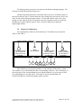
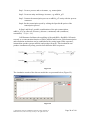
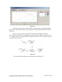
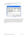
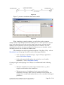
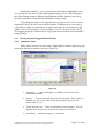
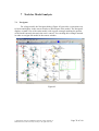
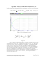
Figure 10
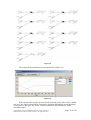
The equations for quantity changes are:
−
dm1
dm 2
= 2,
=1
dt
dt
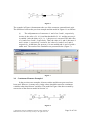
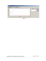
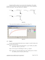
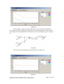
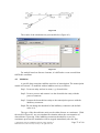
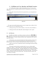
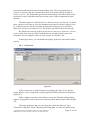
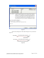
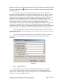
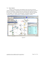
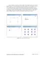
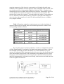
The results of the simulation are presented below (Figure 11).
Figure 11
3.9
Continuous Elements Example 2
In the previous two examples, discrete examples were converted into
similar models with continuous elements. For kinetic based modeling, one should
use a continuous model rather than a discrete one.
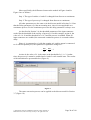
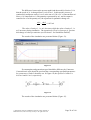
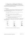
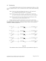
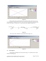
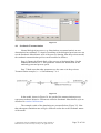
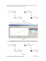
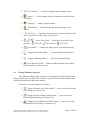
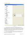
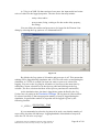
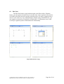
In the following model (Figure 12), the consumption ratio of e1 is
proportional to the value of e1, i.e. the speed of process p1 follows the mass action
kinetics.
Figure 12
© 2002-2008 GNI Ltd. and Human Genome Center, Institute of
Medical Science, The University of Tokyo. All rights reserved.
Page 21 of 100