Download Software Visualization in Prolog

Software Visualization in Prolog
Calum A. McK. Grant
Queens’ College, Cambridge
Dissertation submitted for the degree of Doctor of Philosphy
December 1999
c Calum Grant 1999.
Copyright c Calum Grant 1999.
Vmax and SVT are copyright All rights reserved. Permission is hereby granted to distribute this document without modification in any format or electronic storage system.
Declaration
This dissertation is the result of my own work and includes nothing which is the outcome of work
done in collaboration.
I hereby declare that my dissertation/thesis entitled Software Visualization in Prolog is not
substantially the same as any that I have submitted for a degree or diploma or other qualification
at any other University. I further state that no part of my dissertation/thesis has already been or
is being concurrently submitted for any such degree, diploma or other qualification.
This dissertation is approximately 44 000 words long, excluding appendices.
Acknowledgments
Thanks to everyone who has helped me complete this work, and in particular Peter Robinson my
supervisor, the EPSRC for funding this work, the proof-readers, and all members of the Rainbow
Group for their help and ideas. Thanks also to the departmental secretaries and to my parents.
Trademarks
AVS Express is a registered trademark of Advanced Visual Systems, Inc.
Borland is a registered trademark of Inprise Corp.
C++ Builder is a trademark of Inprise Corp.
Delphi is a trademark of Inprise Corp.
Genitor is a registered trademark of Genitor Corp.
IBM Visualization Data Explorer is a trademark of International Business Machines, Inc.
Java is a trademark of Sun Microsystems, Inc.
LabVIEW is a trademark of National Instruments, Corp.
Linux is a registered trademark of Linus Torvalds.
Microsoft is a registered trademark of Microsoft Corp.
Motif is a trademark of Open Software Foundation, Inc.
OpenGL is a registered trademark of Silicon Graphics, Inc.
Open Inventor is a trademark of Silicon Graphics, Inc.
Pentium is a trademark of Intel Corp.
Prograph is a trademark of Pictorius International.
UNIX is a trademark of X/Open Company, Ltd.
Visual Basic is a trademark of Microsoft Corp.
Visual FoxPro is a trademark of Microsoft Corp.
Visual Studio is a trademark of Microsoft Corp.
Windows is a trademark of Microsoft Corp.
X Window System is a trademark of Massachusetts Institute of Technology.
All other trademarks are the properties of their respective owners.
2
Software Visualization in Prolog
Calum A. McK. Grant
Abstract
Software visualization (SV) uses computer graphics to communicate the structure
and behaviour of complex software and algorithms. One of the important issues in
this field is how to specify SV, because existing systems are very cumbersome to
specify and implement, which limits their effectiveness and hinders SV from being
integrated into professional software development tools.
In this dissertation the visualization process is decomposed into a series of formal
mappings, which provides a formal foundation, and allows separate aspects of visualization to be specified independently. The first mapping specifies the information
content of each view. The second mapping specifies a graphical representation of
the information, and a third mapping specifies the graphical components that make
up the graphical representation. By combining different mappings, completely different views can be generated.
The approach has been implemented in Prolog to provide a very high level specification language for information visualization, and a knowledge engineering environment that allows data queries to tailor the information in a view. The output is
generated by a graphical constraint solver that assembles the graphical components
into a scene.
This system provides a framework for SV called Vmax. Source code and run-time
data are analyzed by Prolog to provide access to information about the program
structure and run-time data for a wide range of highly interconnected browsable
views. Different views and means of visualization can be selected from menus.
An automatic legend describes each view, and can be interactively modified to customize how data is presented. A text window for editing source code is synchronized
with the graphical view. Vmax is a complete Java development environment and end
user SV system.
Vmax compares favourably to existing SV systems in many taxonometric criteria,
including automation, scope, information content, graphical output form, specification, tailorability, navigation, granularity and elision control. The performance and
scalability of the new approach is very reasonable.
We conclude that Prolog provides a formal and high level specification language that
is suitable for specifying all aspects of a SV system.
3
4
Contents
1 Introduction
1.1 Aims . . . . . . . . . . .
1.2 Work Done . . . . . . .
1.3 Results . . . . . . . . . .
1.4 Contribution . . . . . . .
1.5 Notation and Typography
1.6 Dissertation Overview .
.
.
.
.
.
.
.
.
.
.
.
.
.
.
.
.
.
.
.
.
.
.
.
.
.
.
.
.
.
.
.
.
.
.
.
.
.
.
.
.
.
.
.
.
.
.
.
.
2 Previous Work
2.1 Basic Definitions . . . . . . . . . . . .
2.2 Benefits of Software Visualization . . .
2.3 Taxonomies of Software Visualization .
2.4 Software Visualization Systems . . . .
2.4.1 Development Tools . . . . . . .
2.4.2 Visual Programming Systems .
2.4.3 Code Visualization Systems . .
2.4.4 Algorithm Animation Systems .
2.4.5 Run-time Visualization Systems
2.4.6 Architectures . . . . . . . . . .
2.5 Specification . . . . . . . . . . . . . .
2.5.1 Visual Language Theory . . . .
2.5.2 Numerical Data . . . . . . . . .
2.5.3 Specification Languages for SV
2.6 Information Visualization . . . . . . . .
2.6.1 Perception . . . . . . . . . . .
2.6.2 Representations . . . . . . . . .
2.6.3 Architectures . . . . . . . . . .
2.6.4 Graphical Layout . . . . . . . .
2.7 Research Directions . . . . . . . . . . .
2.8 Conclusions . . . . . . . . . . . . . . .
3 A Model of Information Visualization
3.1 Introduction . . . . . . . . . . . .
3.2 Representing Data . . . . . . . . .
3.3 Specifying View Content . . . . .
3.4 Specifying Visual Content . . . .
3.5 A Visual Type System . . . . . . .
.
.
.
.
.
.
.
.
.
.
5
.
.
.
.
.
.
.
.
.
.
.
.
.
.
.
.
.
.
.
.
.
.
.
.
.
.
.
.
.
.
.
.
.
.
.
.
.
.
.
.
.
.
.
.
.
.
.
.
.
.
.
.
.
.
.
.
.
.
.
.
.
.
.
.
.
.
.
.
.
.
.
.
.
.
.
.
.
.
.
.
.
.
.
.
.
.
.
.
.
.
.
.
.
.
.
.
.
.
.
.
.
.
.
.
.
.
.
.
.
.
.
.
.
.
.
.
.
.
.
.
.
.
.
.
.
.
.
.
.
.
.
.
.
.
.
.
.
.
.
.
.
.
.
.
.
.
.
.
.
.
.
.
.
.
.
.
.
.
.
.
.
.
.
.
.
.
.
.
.
.
.
.
.
.
.
.
.
.
.
.
.
.
.
.
.
.
.
.
.
.
.
.
.
.
.
.
.
.
.
.
.
.
.
.
.
.
.
.
.
.
.
.
.
.
.
.
.
.
.
.
.
.
.
.
.
.
.
.
.
.
.
.
.
.
.
.
.
.
.
.
.
.
.
.
.
.
.
.
.
.
.
.
.
.
.
.
.
.
.
.
.
.
.
.
.
.
.
.
.
.
.
.
.
.
.
.
.
.
.
.
.
.
.
.
.
.
.
.
.
.
.
.
.
.
.
.
.
.
.
.
.
.
.
.
.
.
.
.
.
.
.
.
.
.
.
.
.
.
.
.
.
.
.
.
.
.
.
.
.
.
.
.
.
.
.
.
.
.
.
.
.
.
.
.
.
.
.
.
.
.
.
.
.
.
.
.
.
.
.
.
.
.
.
.
.
.
.
.
.
.
.
.
.
.
.
.
.
.
.
.
.
.
.
.
.
.
.
.
.
.
.
.
.
.
.
.
.
.
.
.
.
.
.
.
.
.
.
.
.
.
.
.
.
.
.
.
.
.
.
.
.
.
.
.
.
.
.
.
.
.
.
.
.
.
.
.
.
.
.
.
.
.
.
.
.
.
.
.
.
.
.
.
.
.
.
.
.
.
.
.
.
.
.
.
.
.
.
.
.
.
.
.
.
.
.
.
.
.
.
.
.
.
.
.
.
.
.
.
.
.
.
.
.
.
.
.
.
.
.
.
.
.
.
.
.
.
.
.
.
.
.
.
.
.
.
.
.
.
.
.
.
.
.
.
.
.
.
.
.
.
.
.
.
.
.
.
.
.
.
.
.
.
.
.
.
.
.
.
.
.
.
.
.
.
.
.
.
.
.
.
.
.
.
.
.
.
.
.
.
.
.
.
.
.
.
.
.
.
.
.
.
.
.
.
.
.
.
.
.
.
.
.
.
.
.
.
.
.
.
.
.
.
.
.
.
.
.
.
.
.
.
.
.
.
.
.
.
.
.
.
.
.
.
.
.
.
.
.
.
.
.
.
.
.
.
.
.
.
.
.
.
.
.
.
.
.
.
.
.
.
.
.
.
.
.
.
.
.
.
.
.
.
.
.
.
.
.
.
.
.
.
.
.
.
.
.
.
.
.
.
.
.
.
11
12
13
14
14
16
16
.
.
.
.
.
.
.
.
.
.
.
.
.
.
.
.
.
.
.
.
.
17
17
18
19
22
22
25
25
27
31
32
33
33
34
34
34
35
35
36
36
36
37
.
.
.
.
.
39
39
41
42
44
46
6
CONTENTS
3.6
Specifying Graphical Constraints . . . . . . . . . . . . . . . . . . . . . . . . . . 48
3.7
Generating Views . . . . . . . . . . . . . . . . . . . . . . . . . . . . . . . . . . 49
3.8
Specifying Interaction . . . . . . . . . . . . . . . . . . . . . . . . . . . . . . . . 50
3.9
3.8.1
Actions . . . . . . . . . . . . . . . . . . . . . . . . . . . . . . . . . . . 50
3.8.2
Reactions . . . . . . . . . . . . . . . . . . . . . . . . . . . . . . . . . . 51
Chapter Summary . . . . . . . . . . . . . . . . . . . . . . . . . . . . . . . . . . 52
4 Semantic Visualization Tool
53
4.1
Introduction . . . . . . . . . . . . . . . . . . . . . . . . . . . . . . . . . . . . . 53
4.2
Architecture . . . . . . . . . . . . . . . . . . . . . . . . . . . . . . . . . . . . . 54
4.3
Running SVT . . . . . . . . . . . . . . . . . . . . . . . . . . . . . . . . . . . . 54
4.4
View Manipulation . . . . . . . . . . . . . . . . . . . . . . . . . . . . . . . . . 55
4.5
Generating Visualizations . . . . . . . . . . . . . . . . . . . . . . . . . . . . . . 56
4.6
4.5.1
Acquiring the Visual Primitives . . . . . . . . . . . . . . . . . . . . . . 57
4.5.2
Generating the Scene Graph . . . . . . . . . . . . . . . . . . . . . . . . 58
4.5.3
Structuring The Scene Graph . . . . . . . . . . . . . . . . . . . . . . . . 58
4.5.4
Graphical Layout . . . . . . . . . . . . . . . . . . . . . . . . . . . . . . 60
4.5.5
Graphical Layout Algorithms . . . . . . . . . . . . . . . . . . . . . . . 60
Expanding the Graphical Vocabulary . . . . . . . . . . . . . . . . . . . . . . . . 62
4.6.1
4.7
4.8
4.9
Specifying Visual Objects . . . . . . . . . . . . . . . . . . . . . . . . . 64
Interaction . . . . . . . . . . . . . . . . . . . . . . . . . . . . . . . . . . . . . . 69
4.7.1
Disambiguating Actions . . . . . . . . . . . . . . . . . . . . . . . . . . 70
4.7.2
Menus . . . . . . . . . . . . . . . . . . . . . . . . . . . . . . . . . . . . 71
4.7.3
Navigation . . . . . . . . . . . . . . . . . . . . . . . . . . . . . . . . . 71
4.7.4
Selecting Graphical Form . . . . . . . . . . . . . . . . . . . . . . . . . 72
4.7.5
Modifying the Action Relation . . . . . . . . . . . . . . . . . . . . . . . 73
The Legend . . . . . . . . . . . . . . . . . . . . . . . . . . . . . . . . . . . . . 75
4.8.1
Displaying the Legend . . . . . . . . . . . . . . . . . . . . . . . . . . . 76
4.8.2
Modifying the Visualization Relation . . . . . . . . . . . . . . . . . . . 76
The Bookmarks . . . . . . . . . . . . . . . . . . . . . . . . . . . . . . . . . . . 77
4.10 The Preview Window . . . . . . . . . . . . . . . . . . . . . . . . . . . . . . . . 77
4.11 Chapter Summary . . . . . . . . . . . . . . . . . . . . . . . . . . . . . . . . . . 79
5 A Tool for Software Visualization
81
5.1
Introduction . . . . . . . . . . . . . . . . . . . . . . . . . . . . . . . . . . . . . 81
5.2
Architecture . . . . . . . . . . . . . . . . . . . . . . . . . . . . . . . . . . . . . 82
5.3
Text Processing . . . . . . . . . . . . . . . . . . . . . . . . . . . . . . . . . . . 82
5.4
Directory Visualization . . . . . . . . . . . . . . . . . . . . . . . . . . . . . . . 84
5.4.1
5.5
5.6
MIME Types . . . . . . . . . . . . . . . . . . . . . . . . . . . . . . . . 88
Analyzing Java Source Code . . . . . . . . . . . . . . . . . . . . . . . . . . . . 88
5.5.1
Constructing the Program Database . . . . . . . . . . . . . . . . . . . . 88
5.5.2
Analyzing the Program Database . . . . . . . . . . . . . . . . . . . . . . 90
Java Visualization . . . . . . . . . . . . . . . . . . . . . . . . . . . . . . . . . . 91
5.6.1
Visualizing Files, Classes and Packages . . . . . . . . . . . . . . . . . . 91
5.6.2
Visualizing Cross-references . . . . . . . . . . . . . . . . . . . . . . . . 99
5.6.3
Visualizing Methods . . . . . . . . . . . . . . . . . . . . . . . . . . . . 104
CONTENTS
5.7
7
Analyzing Run-time Data . . . . . . . . . . . . . . . . . . . . . . . . . . . . . . 113
5.7.1
Adding Trace Points . . . . . . . . . . . . . . . . . . . . . . . . . . . . 113
5.7.2
Generating the Trace File . . . . . . . . . . . . . . . . . . . . . . . . . . 113
5.7.3
Reading the Trace File . . . . . . . . . . . . . . . . . . . . . . . . . . . 115
5.8
Run-time Data Visualization . . . . . . . . . . . . . . . . . . . . . . . . . . . . 116
5.9
Prolog Visualization . . . . . . . . . . . . . . . . . . . . . . . . . . . . . . . . . 127
5.9.1 Editing Prolog . . . . . . . . . . . . . . . . . . . . . . . . . . . . . . . 129
5.8.1
Value Visualization . . . . . . . . . . . . . . . . . . . . . . . . . . . . . 120
5.10 The Help System . . . . . . . . . . . . . . . . . . . . . . . . . . . . . . . . . . 131
5.11 Chapter Summary . . . . . . . . . . . . . . . . . . . . . . . . . . . . . . . . . . 133
6 Discussion
6.1
6.2
6.3
135
Classifying Vmax . . . . . . . . . . . . . . . . . . . . . . . . . . . . . . . . . . 135
6.1.1
Scope . . . . . . . . . . . . . . . . . . . . . . . . . . . . . . . . . . . . 135
6.1.2
Content . . . . . . . . . . . . . . . . . . . . . . . . . . . . . . . . . . . 137
6.1.3
Form . . . . . . . . . . . . . . . . . . . . . . . . . . . . . . . . . . . . 137
6.1.4
6.1.5
Method . . . . . . . . . . . . . . . . . . . . . . . . . . . . . . . . . . . 138
Interaction . . . . . . . . . . . . . . . . . . . . . . . . . . . . . . . . . 139
6.1.6
Effectiveness . . . . . . . . . . . . . . . . . . . . . . . . . . . . . . . . 139
Evaluating Vmax . . . . . . . . . . . . . . . . . . . . . . . . . . . . . . . . . . 139
6.2.1
Benefits . . . . . . . . . . . . . . . . . . . . . . . . . . . . . . . . . . . 140
6.2.2
Performance . . . . . . . . . . . . . . . . . . . . . . . . . . . . . . . . 140
6.2.3
Extensibility . . . . . . . . . . . . . . . . . . . . . . . . . . . . . . . . 141
Evaluating SVT . . . . . . . . . . . . . . . . . . . . . . . . . . . . . . . . . . . 141
6.3.1
The Specification Language . . . . . . . . . . . . . . . . . . . . . . . . 141
6.3.2
Modularity . . . . . . . . . . . . . . . . . . . . . . . . . . . . . . . . . 142
6.3.3
Application Areas . . . . . . . . . . . . . . . . . . . . . . . . . . . . . 142
6.4
Commercial Relevance . . . . . . . . . . . . . . . . . . . . . . . . . . . . . . . 143
6.5
Further Work . . . . . . . . . . . . . . . . . . . . . . . . . . . . . . . . . . . . 145
6.5.1
6.5.2
Measure Usability of Vmax . . . . . . . . . . . . . . . . . . . . . . . . 145
Measure Programmers’ Needs . . . . . . . . . . . . . . . . . . . . . . . 145
6.5.3
Improve the Graphical Constraint Solver . . . . . . . . . . . . . . . . . 146
6.5.4
Animation . . . . . . . . . . . . . . . . . . . . . . . . . . . . . . . . . 146
6.5.5
Sound . . . . . . . . . . . . . . . . . . . . . . . . . . . . . . . . . . . . 146
6.5.6
Automatic Choice of Graphical Layout . . . . . . . . . . . . . . . . . . 146
6.5.7
Improve the Graphical User Interface . . . . . . . . . . . . . . . . . . . 146
6.5.8
Investigate other Specification Languages . . . . . . . . . . . . . . . . . 146
6.5.9
Investigate Visual Specification Languages . . . . . . . . . . . . . . . . 147
6.5.10 Natural Language Interface . . . . . . . . . . . . . . . . . . . . . . . . . 147
6.5.11 Formal Theory of Visualization . . . . . . . . . . . . . . . . . . . . . . 147
6.5.12 Improve Program Analysis . . . . . . . . . . . . . . . . . . . . . . . . . 148
6.5.13 Visualize other Languages, such as C++ . . . . . . . . . . . . . . . . . . 148
6.5.14 Data Persistence . . . . . . . . . . . . . . . . . . . . . . . . . . . . . . 148
6.5.15 Provide Visual Programming . . . . . . . . . . . . . . . . . . . . . . . . 148
6.5.16 Interface to Compilers . . . . . . . . . . . . . . . . . . . . . . . . . . . 148
6.5.17 Interface to the Java Virtual Machine Debug Interface . . . . . . . . . . . 148
8
CONTENTS
6.5.18 Improve Efficiency . . . . . . . . . . . . . . . . . . . . . . . . . . . . . 148
6.6
Chapter Summary . . . . . . . . . . . . . . . . . . . . . . . . . . . . . . . . . . 149
7 Conclusions
151
7.1 Vmax . . . . . . . . . . . . . . . . . . . . . . . . . . . . . . . . . . . . . . . . 151
7.1.1
7.1.2
Strengths of Vmax . . . . . . . . . . . . . . . . . . . . . . . . . . . . . 151
Weaknesses of Vmax . . . . . . . . . . . . . . . . . . . . . . . . . . . . 152
7.2
Implementing SV Systems . . . . . . . . . . . . . . . . . . . . . . . . . . . . . 152
7.3
7.4
Specifying SV Systems . . . . . . . . . . . . . . . . . . . . . . . . . . . . . . . 153
The Role of Prolog in Software Visualization . . . . . . . . . . . . . . . . . . . 153
7.4.1
7.4.2
Advantages of using Prolog as a Specification Language . . . . . . . . . 154
Disadvantages of Prolog . . . . . . . . . . . . . . . . . . . . . . . . . . 154
7.5
Information Visualization in SVT . . . . . . . . . . . . . . . . . . . . . . . . . 155
7.5.1 Formalizing Information Visualization . . . . . . . . . . . . . . . . . . . 155
7.6
Contribution . . . . . . . . . . . . . . . . . . . . . . . . . . . . . . . . . . . . . 155
7.7
Future Directions . . . . . . . . . . . . . . . . . . . . . . . . . . . . . . . . . . 155
A Definitions
163
B Documentation
165
B.1 Running SVT . . . . . . . . . . . . . . . . . . . . . . . . . . . . . . . . . . . . 165
B.2 SVT Predicate Summary . . . . . . . . . . . . . . . . . . . . . . . . . . . . . . 165
B.2.1 View Predicates . . . . . . . . . . . . . . . . . . . . . . . . . . . . . . . 166
B.2.2
Visualization Predicates . . . . . . . . . . . . . . . . . . . . . . . . . . 166
B.2.3
B.2.4
Legend Predicates . . . . . . . . . . . . . . . . . . . . . . . . . . . . . 167
Interaction Predicates . . . . . . . . . . . . . . . . . . . . . . . . . . . . 168
B.2.5
B.2.6
Text Predicates . . . . . . . . . . . . . . . . . . . . . . . . . . . . . . . 168
Miscellaneous Predicates . . . . . . . . . . . . . . . . . . . . . . . . . . 169
B.3 Vmax Predicate Summary . . . . . . . . . . . . . . . . . . . . . . . . . . . . . 170
B.3.1 Filing System . . . . . . . . . . . . . . . . . . . . . . . . . . . . . . . . 170
B.3.2
Java Source Code . . . . . . . . . . . . . . . . . . . . . . . . . . . . . . 171
B.3.3
B.3.4
Java Run-time . . . . . . . . . . . . . . . . . . . . . . . . . . . . . . . 175
Prolog Source Code . . . . . . . . . . . . . . . . . . . . . . . . . . . . 176
B.4 Visuals Defined by SVT . . . . . . . . . . . . . . . . . . . . . . . . . . . . . . 176
B.5 Visual Object Components Defined by SVT . . . . . . . . . . . . . . . . . . . . 176
B.6 Graphical Constraints Defined by SVT . . . . . . . . . . . . . . . . . . . . . . . 177
B.7 Actions Defined by SVT . . . . . . . . . . . . . . . . . . . . . . . . . . . . . . 178
B.8 Views Defined by Vmax . . . . . . . . . . . . . . . . . . . . . . . . . . . . . . 178
B.9 The C++ Interface . . . . . . . . . . . . . . . . . . . . . . . . . . . . . . . . . . 179
B.9.1 Adding Graphical Constraints . . . . . . . . . . . . . . . . . . . . . . . 179
B.9.2
The Graphical User Interface . . . . . . . . . . . . . . . . . . . . . . . . 181
C Further Examples
183
C.1 Views . . . . . . . . . . . . . . . . . . . . . . . . . . . . . . . . . . . . . . . . 183
C.2 Visualization Relations . . . . . . . . . . . . . . . . . . . . . . . . . . . . . . . 184
C.3 Visuals . . . . . . . . . . . . . . . . . . . . . . . . . . . . . . . . . . . . . . . . 185
C.4 Visual Objects . . . . . . . . . . . . . . . . . . . . . . . . . . . . . . . . . . . . 186
CONTENTS
C.5 Interaction . . . . . . . . . . . . . .
C.5.1 Menus . . . . . . . . . . . .
C.5.2 An Implementation of CCS
C.6 A Scientific Calculator . . . . . . .
9
.
.
.
.
.
.
.
.
.
.
.
.
.
.
.
.
.
.
.
.
.
.
.
.
.
.
.
.
.
.
.
.
.
.
.
.
.
.
.
.
.
.
.
.
.
.
.
.
.
.
.
.
.
.
.
.
.
.
.
.
.
.
.
.
.
.
.
.
.
.
.
.
.
.
.
.
.
.
.
.
.
.
.
.
.
.
.
.
.
.
.
.
.
.
.
.
187
188
188
189
10
CONTENTS
Chapter 1
Introduction
Computer software has revolutionized the way we work, and the software industry is worth
trillions of dollars world wide. Software systems are the most complex artificial objects ever
constructed, and managing their complexity is difficult. Software is also very difficult to write,
understand and debug. In response, software tools are rapidly evolving to create software more
quickly and reliably.
One approach to the problems of comprehension and complexity is through computer graphics
and visualization. This is software visualization (SV), which encompasses all applications of
graphics to software development, including static program visualization, visual programming
(manipulating graphical representations of code), and visualization of run-time behaviour.
The rationale for SV is that programmers and managers need to understand a software system,
often long after it was written, for debugging and updating. It is widely accepted that code
maintenance is the most expensive part of software engineering [94]. Even small algorithms
can be difficult to understand, debug, or communicate to students. Computer graphics offers a
powerful means of communicating that information through visualization.
The Year 2000 Bug highlights the need for SV. A programmer trying to debug poorly documented legacy code would wish to know not just the overall structure of the program, but the
dependencies of the various functions in the system, which variables stored dates, and even which
functions or statements apply date calculations. Using SV, a program analysis would determine
this information and display it in graphical form.
Although development tools have provided enormous productivity gains, their degree of visualization is still very limited, and visual programming has not proved as successful as was
initially hoped [107]. The recent advances in software development tools have come from improved user interfaces and graphical support, and SV could improve that productivity further.
In spite of the obvious benefits, there are considerable technical difficulties to overcome. The
main problem preventing SV from being used in professional development tools is its inflexibility and high set up costs. A system for automatic SV is needed to make SV accessible to
programmers. At the same time it should be flexible enough to provide the desired information
is the desired format. In general, SV systems are either automatic or flexible - they are not both
[64].
The aim of a SV system is to provide useful information about a program to a user. Programmers need many different types of information, so complete systems should visualize all aspects
of software, including the program structure, low level details, high level overviews and run-time
data. Most SV systems are very specific, and have a very limited scope. In addition they have a
very poor range of granularity, and do not view the program on many different levels of detail.
The elision control of most SV systems is very poor, and there are no facilities for filtering away
irrelevant information, or for the user to specify what is or isn’t of interest.
Existing SV tools or development environments have a very limited number of views of program objects or output data. In fact, there are dozens of different ways of representing every program object, each conveying different information, or using different visualization techniques.
11
12
1.1. AIMS
Many SV systems only have fixed output, and changing the output requires manual programming, which hinders end users from tailoring their views. The mapping from data to graphical
form is fixed by programming or specification languages in SV systems, but techniques for allowing users to change this mapping interactively would allow end users to customize the views
themselves.
Interaction with SV systems is also very limited. Most views are not interactive so the objects
in the view cannot be interacted with. For example it might be useful to display information
about objects beneath the mouse cursor, or to provide a graphical display of whatever lies beneath
the mouse cursor. It might also be useful to display an automatic legend of each view because
views containing many different types of graphical structures can be confusing. Better navigation
techniques would allow programmers to browse software and find information more quickly.
There is little theory that underpins SV. Current approaches do not use any theoretical basis,
and are implemented ad hoc. Work should be done on the formalization of information display,
which might lead to more principled methods for designing SV systems.
The specification techniques for SV systems are very awkward. SV systems are specified at
a very low level, and they are therefore cumbersome to use. Work on specification languages
is needed to provide high level specification and scripting of SV, which would make SV much
easier to implement, and provide much more powerful systems.
In spite of these technical difficulties, SV systems provide valuable insights into the workings
of complex software for many different kinds of computer language and task. The challenge
SV presents is to provide a system which is very broad in scope, very flexible in its output, has
dozens of different types of view, is completely automatic, can be interactively customized, and
can be specified at a high level.
1.1
Aims
Price et al. [79] identify many of these difficulties and outline directions for future work. The
aim of this work is to produce a SV system that addresses some of these problems by achieving
the following aims:
1. Have a broad scope, visualizing all aspects of computer software. Previous systems are
too limited in their scope. Aspects to include are:
Program structure.
Object orientation.
Methods.
Run-time data.
Results from program analysis, such as method calls, variable uses and cross references.
2. Provide a high level specification method. This should specify the following aspects of
SV:
View content - what a view is showing. This must provide a generic query mechanism.
Graphical abstraction - how the contents of the view are rendered.
Interaction - how to interact with items in the view.
The specification methods of existing systems are very awkward to use, and do not specify
either view content or interaction.
3. Provide dozens of different views of the program and run-time data. Previous systems
provide only a small number of views because of the difficulties in setting up new views.
CHAPTER 1. INTRODUCTION
13
4. Base the implementation on a theoretical foundation. Existing SV systems are not based
on formal models.
5. Provide a rich and varied graphical output. This offers a more powerful and interesting
means of expression.
6. Provide flexibility in graphical representation. Users should be able to interactively change
the way data is represented.
7. Provide a legend that describes the contents of the view. This is necessary if the graphical
representation is so flexible, and useful for users unfamiliar with the system. No other
systems provide an automatic legend.
8. Provide navigation by browsing to program objects in the scene. Provide a preview window that graphically displays the object beneath the mouse cursor, and graphical bookmarks that store views for later retrieval. Such an interface would provide an easy means
to access data.
9. Provide a text editing window that is synchronized with graphical views of the source code.
This would provide code browsing and a complete development environment.
1.2
Work Done
These aims have been met by redesigning the visualization engine that sits at the core of the SV
system to generate the views.
A specification method for information visualization has been developed by decomposing the
visualization process into a series of relations that can be specified in Prolog. This provides a
formal foundation to information visualization, and therefore to SV. The formal model is called
a semantic model because the information content of a view, or its semantics, is always defined
explicitly. The model also incorporates a formal model of interaction with visualizations.
This method has been shown to be practical by implementing a general purpose information
visualization tool, Semantic Visualization Tool (SVT), using this approach. SVT can in principle be used for for any type of visualization, and it is specified entirely in Prolog. It provides
a method for interfacing any knowledge based environment in Prolog to any graphical output
algorithm.
SVT abstracts the information content of a view from its graphical representation. The mapping from the information content to the graphical representation is dynamic, so that different
mappings can be selected from a menu to render the information differently. The mapping can
be queried, so that a legend can automatically describe what is in the view. The mapping can be
completely tailored by the user by interacting with the legend to change the way individual items
are graphically represented.
SVT provides a browser interface so that any item in a view is navigated to by clicking on
it. Alternative queries of the current object being viewed can be selected from a menu, and
alternative methods of visualizing the current information can also be selected from a menu.
A preview window automatically provides a graphical display of the object beneath the mouse
cursor, and a bookmark window provides five thumbnail views that can be used to store and
retrieve views.
SVT provides a framework for SV. A system called Vmax has been implemented to browse
Java source code and Java run-time data. Vmax is specified in Prolog, and uses Prolog to analyze
source code and run-time data and store the program database. Views defined in Vmax can query
the program database to provide any information about the program.
SVT provides Vmax with a specification language that allows all aspects of SV to be specified at a high level. SVT also automatically manages navigation and the legend, and provides
graphical algorithms to display the output.
Vmax has a text editor to edit source code, and provides a complete development environment
with integrated end-user SV. Vmax can be extended by loading users’ Prolog. Vmax also visu-
14
1.3. RESULTS
alizes Prolog, and can edit Prolog as a visual language, so that users can write their own queries
visually to provide new views.
Prolog can specify other types of visualization, such as directory browsing and graphical user
interfaces. SVT and Vmax were implemented to investigate whether using Prolog is a realistic
approach to SV, and how such a system would be designed.
1.3
Results
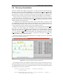
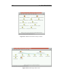
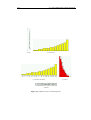
SVT and Vmax provide a comprehensive SV environment. Because the approach is generic, the
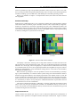
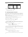
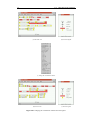
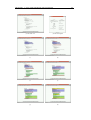
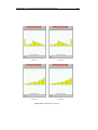
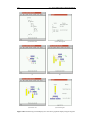
system has a very broad scope and a very wide range of graphical output form. Figure 1.1 shows
a range of sample output.
On a modern desktop PC, the performance of Vmax is quite reasonable, making it suitable
for visualizing projects of around 100 000 lines of code. The code input rate is about 6 300
lines of Java per second. The time to generate views is typically under half a second. The final
system has 151 different types of view, or 70 if alternative visualizations are discounted. These
include 44 views for Java source code, 7 views for Java run-time, 8 views for Prolog, 6 views for
directories and one view for help.
A taxonometric classification of Vmax has been made using the taxonomy of Price et al. [79],
given in Table 6.1. It shows the new approach to compare favourably to previous systems in many
criteria including automation, scope, information content, graphical output form, specification,
tailorability, navigation, granularity and elision control.
An empirical study of usability and usefulness of the system lies beyond the scope of this
work. It is intended only to demonstrate new techniques, and there are no standard methods for
empirical evaluation of SV systems. The system is easy to use due to its browser interface and
degree of automation, but this has not been confirmed by usability studies.
The reader is invited to download Vmax. 1
1.4
Contribution
The work demonstrates a number of new techniques that can be applied to SV.
It has been demonstrated that the programming language Prolog can be used to specify all
aspects of SV.
A SV system has been constructed that compares favourably to existing systems in many
taxonometric criteria, including scope, information content, graphical output form, specification, tailorability, navigation, granularity and elision control.
A semantic model of information visualization provides a link between visualization, first
order logic, and knowledge engineering. Visualization systems and knowledge engineering systems can be integrated.
A general purpose information visualization tool has been implemented that can be specified entirely in Prolog.
A dynamic mapping between the information content of a view and the graphical form of
a view has been implemented. This can be queried to provide an automatic legend, and
modified by the user. Different mappings can be selected to tailor the output.
A type system for information artefacts [38] and graphical artefacts has been implemented.
Visual languages can be specified in Prolog.
New methods of interaction have been demonstrated, including a browser interface to navigate around a program database, a legend, and a preview window.
1 URL:
http://www.cl.cam.ac.uk/Research/Rainbow/vmax
CHAPTER 1. INTRODUCTION
15
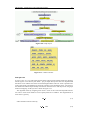
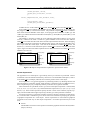
(a) Method control flow.
(b) Method block structure.
(c) Class hierarchy.
(d) Cross referencing.
(e) Run-time data in a graph.
(f) Run-time data in a table.
(g) Prolog visualization.
(h) GUI specification.
Figure 1.1. The scope and output of Vmax.
16
1.5. NOTATION AND TYPOGRAPHY
1.5
New visualizations for program objects, including coloured Nassi Shneiderman Diagrams
[72], have been developed.
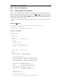
Notation and Typography
Text that is written in a slanted font refers to Prolog or C++ source code. e.g. virtual void
On reset size();
Text inset in a Courier font is a larger example of Prolog or C++ source code. e.g.
// This is C++ source code
1.6
Prolog atoms and functors begin with a lowercase letter. e.g. charles or parent(charles,
harry).
Prolog compound terms are written as a functor followed by a comma-delimited list of
arguments in round brackets. e.g. parent(charles, harry).
Prolog lists are written in square brackets. e.g. [1, 2, 3].
Prolog variables begin with an uppercase letter. e.g. X, Id and Object4. The variable ‘ ’ is
unbound.
Prolog predicates or compound terms may written as Functor/Arity. e.g. parent(Parent,
Child) would be written parent/2. parent/2 is understood to be distinct from parent/3.
Prolog modules are written as Module:Predicate. e.g. java:method(Method). Often the
module prefix is omitted.
Dissertation Overview
Chapter 2 describes the previous work in the field, from SV systems and visual programming, to
the state of the art in commercial systems. The taxonomies of SV [79, 84] and visual programming [71] provide important reference points for future work, and have motivated much of this
work.
Chapter 3 describes a formal model of information visualization, and how visualization can be
specified in Prolog. This is the theory that underlies the rest of the work. Chapter 4 describes how
the model and specification techniques described in Chapter 3 can be implemented in practice. A
generic visualization tool, Semantic Visualization Tool, is developed that can be used to visualize
any kind of data, including the structured and relational data in computer software.
Chapter 5 describes Vmax, a tool for software visualization, that is the main product of this
work. Chapter 6 presents the results and evaluation of this work and discusses where Vmax fits
in to the taxonomies of SV. The conclusions are in Chapter 7.
The appendices contain documentation for SVT and Vmax, and further examples to illustrate
the specification techniques.
Chapter 2
Previous Work
Although computer programming is traditionally a textual discipline, the use of
graphical illustrations of software has always played a useful role in software development and writing computer programs. Illustrations are used to plan and document software, although the idea of using illustrations to create programs (visual
programming) has been around for a long time [99], as well as automated utilities to
document and browse finished software. Visual techniques are now commonplace
in software development, particularly in the design and generation of user interfaces,
the construction of skeleton applications, and the navigation of source code.
This survey describes the issues and areas of research within software visualization,
a number of systems - both commercial and research - that use software visualization
techniques, and a number of taxonomies for describing and comparing software
visualization systems. The survey concludes with research problems that need to
be solved for software visualization to deliver real demonstrable gains to software
developers.
2.1
Basic Definitions
There is no universal consensus in the literature for the definitions of broad terms such as visual,
visualization, visual programming, software visualization, program visualization and algorithm
animation. Although the concepts themselves are fairly clear, different sources place emphasis
on different concepts in forming their definitions.
The Concise Oxford Dictionary [100] defines visual as “of, concerned with, or used in, seeing,” and visualize as “make visible, esp. to the mind (thing not visible to the eye); make visible to
the eye.” Price et al. [79] prefer the definition “the power or process of forming a mental picture
or vision of something not actually present in sight” from the Oxford English Dictionary [92],
with the emphasis that visualization is a mental process rather than just the task of vision, and
can therefore include all of the senses. This contrasts with the definition given by McCormick et
al. [66] as “the study of mechanisms in computers and in humans which allow them in convert
to perceive, use, and communicate visual information,” with the emphasis clearly on the process
of communication. These definitions are not mutually exclusive because visual communication
precedes the cognitive model. In this text, visual is taken to mean “visible”, and visualization to
mean “conversion to visible form,” even though this excludes the other senses. In the context of
computers, visual means “visible on a computer display,” and visualization is “communicating
data with graphics.” This specifically includes all graphical forms, as well as text, which is of
course visible. These definitions are more straightforward than those offered by Price et al. or
McCormick et al.
Myers [71] defines visual programming (VP) as “any system that allows the user to specify
a program in a two-(or more)-dimensional fashion,” and specifically excludes textual languages
(which he considers to be one-dimensional), picture definition languages and drawing packages.
17
18
2.2. BENEFITS OF SOFTWARE VISUALIZATION
Price et al. define VP as “the use of visual techniques to specify a program in the first place.”
Price’s definition is better because textual languages are visual and have a two-dimensional rendering – Myers confuses the display with the internal representation of the textual language.
Myers distinguishes program visualization (PV) from VP as “the program [being] specified in
a conventional, textual manner, and the graphics is used to illustrate some aspect of the program
or its run-time execution.” Price et al. prefer the term software visualization (SV) to encompass
algorithm animation (animating the operations of an algorithm), code visualization (a visual
form of the program code) and data visualization (a visual form of the program data) and defines
it to be “the use of the crafts of typography, graphic design, animation and cinematography with
modern human-computer interaction technology to facilitate both the human understanding and
effective use of computer software.”
Software Visualization
Algorithm Visualization
Program Visualization
Data Animation
Static Algorithm Visualization
Static
Static
Code
Data
Visual Programming
Visualization
Visualization
Algorithm Animation
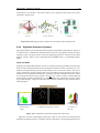
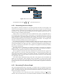
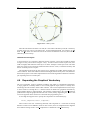
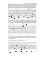
Code Animation
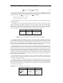
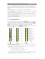
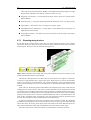
Figure 2.1. Venn Diagram showing relationships between the various fields of software visualization (reproduced from [79]).
Myers excludes VP from PV while Price et al. include it. Price et al. classify the SV fields
and nomenclature according to Figure 2.1, although they concede that their classification is an
oversimplification because these fields are strongly interrelated.
Sometimes products such as Delphi or Visual Basic are regarded as VP, because visual techniques are being used to create software. But these are not VP systems because textual programming is still necessary - navigation and the design of the user interfaces is visual, but that is not
considered to be programming.
The above fields all use visual languages which Myers defines as “all systems that [use]
graphics, including VP and PV systems,” and visual programming languages (VPLs) are visual
languages used for programming. The definitions given by Myers [71] are probably the de facto
standard, but are by no means definitive.
2.2
Benefits of Software Visualization
Visual representations seek, if not always successfully, to assist software development. By providing representations of software that are in some way superior to text, programmers can understand complex software systems more easily, thus decreasing development and debugging effort
and improving documentation and code reuse. Given that software is a trillion dollar industry,
even small gains should be considered important.
There are many claims of the benefits of the visual environments for software development
CHAPTER 2. PREVIOUS WORK
19
and programming. Blackwell [10] looks at the benefits computer scientists perceive of visual
programming, which also apply to software visualization. He analyzes these claims in detail,
and finds a general consensus among computer scientists, although some claims are indeed controversial or counter empirical evidence.
Blackwell found that while few of these claims could be absolute, most had a logical basis
or some supporting evidence, but the claims of superlativism, of being natural and intuitive, of
utilizing more fully human cognitive resources, and of increased information content were unsound. However there are still many potential advantages of using imagery over text, including
increased productivity, concretizing abstract concepts, program structure being more easily conveyed pictorially, assisting the programmer’s mental model of software, and resemblance to the
real world thus utilizing our instinctive manipulative skills [90].
There is some notable opposition to visual languages, which is reasonable in the absence of
much empirical evidence supporting visual programming. Brooks [14] states that “A favorite
subject for Ph.D. dissertations in software engineering is graphical, or visual, programming the application of computer graphics to software design. Nothing even convincing, much less
exciting, has yet emerged from such efforts. I am persuaded that nothing will.” This argument
should not be taken too seriously because it was written before windowing systems, he only considers flow chart techniques, and confuses superimposed views with multiple views. Brooks also
claims that limited size of display renders visual programs unscalable, although this argument
collapses when one considers multiple views. Scaling is indeed a problem in visual languages
[17], but the problem has been overcome in textual languages. O’Brien [73] states “...beware
the claims of visual programming. Drawing lines between objects becomes bafflingly web-like.
Purely visual programming is not yet and may never be viable.” This argument is also flawed
because structured networks (such as those used in LabVIEW [104] or ProGraph [19, 77]) is
just one visual representation of code. The empirical evidence supporting visual programming
languages is discussed at length by Whitley [107].
These arguments are directed at the practicalities of VP where the text in the system has been
replaced entirely by diagrams, rather than at SV. Visual programming has many weaknesses that
need to be overcome, including lack of scalability [17], that visual representations are not as
compact as textual ones [71], awkwardness to edit in visual notation, when text and keyboards
can be faster [36], or that purely visual programming systems are no better than traditional ones
for large projects. The emphasis of current research is to tackle these problems.
In fact Brooks [13] is entirely in favour of using diagrams to assist software development,
and has “enthusiasm for using diagrams as thought and design aids.” Brooks also concedes that
multiple diagrams are required for different aspects of software, and that some aspects are more
suitable for visualization than others. It is the awkwardness of visual representation at the lowest
level (code) that seems to be impeding visual programming. Removing text entirely may indeed
not be desirable or practical, but visual support for software development has proved to be very
useful.
2.3
Taxonomies of Software Visualization
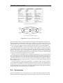
The most comprehensive taxonomy of SV is provided by Price et al. [79]. Myers’s taxonomy [71]
precedes Price’s, and offers taxonomies for VP as well as PV. Roman and Cox [84] offer a simpler
and less comprehensive taxonomy of PV. Taxonomies serve to classify, quantify and describe
types of SV and visualization systems, assist in finding weaknesses and areas of research, and
offer ways of comparing and evaluating SV systems.
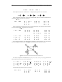
The taxonomies also discuss and classify various SV systems. Price et al. classify and compare in detail twelve systems: Sorting out Sorting [3], Balsa [16], Zeus [15], TANGO [95], ANIM
[8], Pascal Genie (from Chariot Software Group), UWPI [42], SEE [4], TPM [12], Pavane [86],
LogoMedia [25] and CenterLine ObjectCenter [93]. Price et al. then construct a taxonomy based
upon a tree structure, where each leaf in the taxonomy offers a different and orthogonal classification criterion. The complete taxonomy is shown in Figure 2.2.
Price et al. justify their first level classification by a generalized model of the software vi-
20
2.3. TAXONOMIES OF SOFTWARE VISUALIZATION
Hardware
Operating System
Generality
Scope
Language
Concurrency
Applications
Speciality
Program
Scaleablilty
Data Sets
Code
Control Flow
Program
Data
Data Flow
Instructions
Control Flow
Data
Data Flow
Algorithm
Content
Completeness
Invasiveness
Temporal
Gather time
Generation Time
Medium
Colour
Graphical Vocab.
Dimensions
Presentation
Software Visualization
Form
Animation
Sound
Granularity
Elision
Views
Synchronisation
Intelligence
Specification
Tailorability
Language
Method
Ignorance
Connection
Coupling
Style
Elision Control
Interaction
Navigation
Direction
Temporal Control
Speed
Scripting
Purpose
Appropriateness
Effectiveness
Evaluation
Production Use
Figure 2.2. Price et al.’s taxonomy of software visualization.
CHAPTER 2. PREVIOUS WORK
21
sualization process. Scope relates to the source program and the input domain of the software
visualizer. Content describes the particular aspect of the software that is visualized. Form describes the output of the system. Method describes how the implementation is specified and how
the SV system works. Interaction describes how the user can interact with the view or the SV
system to control, navigate, or modify the visualization. Effectiveness offers evaluation criteria for SV systems. By making their taxonomy tree structured they allow their taxonomy to be
extended as the field evolves.
Roman and Cox offer a related taxonomy, shown in Figure 2.3.
Code
Data State
Scope
Control State
Behaviour
Direct Representation
Abstraction
Structural Represenation
Synthesised Rep.
Predefinition
Annotation
Specification
Declaration
Manipulation
Program Visualization
Simple Objects
Composite Objects
Graphical Vocabulary
Visual Events
Worlds
Interface
Multiple Worlds
Through Controls
Interaction
Through the Image
Interpretation of graphics
Analytical Presentation
Presentation
Explanatory Presentation
Orchestration
Figure 2.3. Roman and Cox’s taxonomy of program visualization.
Roman and Cox’s “Scope” category contains Price’s “Scope” and “Content” categories. By
“Abstraction”, Roman and Cox mean the degree to which the code has been transformed. This
overlaps Price’s “Content” and “Form” categories. Roman and Cox’s “Specification” category
is contained within Price’s “Method” category. Roman and Cox’s “Interface” category describes
both rendering and interaction, so contains Price’s “Form” and “Interaction” categories. Roman
and Cox’s “Presentation” category denotes the semantics of the visualization, and is contained
within Price’s “Form” category. Roman and Cox’s taxonomy is awkward here because it separates “Graphical vocabulary” and “Presentation.” Roman and Cox do not consider “Effectiveness” and purpose in their taxonomy, when this is surely one of the most important facts about a
SV system.
Myers [71] offers three different taxonomies, for programming systems, program visualization systems, and language specification technique. He classifies programming systems using
22
2.4. SOFTWARE VISUALIZATION SYSTEMS
three orthogonal criteria, giving eight categories. The criteria are: visual vs. textual programming, example based vs. not example based, and interpreted vs. compiled. The taxonomy for
PV systems uses a 2x3 grid, with static vs. dynamic on one axis, and code visualization, data
visualization and algorithm visualization on the other. A programming system may belong to
more than one category. The taxonomy by specification technique lists 14 different methods of
language specification, and examples of visual languages belonging to each category. Myers’
taxonomies are forerunners to Price et al.’s, which is far more comprehensive and more applicable to SV.
2.4
Software Visualization Systems
A range of SV systems are presented in this section. Unfortunately a comprehensive survey
is beyond the scope of this work. There are hundreds of programming systems using visual
techniques, which are roughly divided into development tools utilizing visual techniques, visual
programming systems, and software visualization systems.
2.4.1
Development Tools
Almost every professional development tool uses visual techniques to assist application development. These visual development tools represent the state of the art commercially, and offer “rapid
application development” compared with text-only environments. These tools form a basis for
more advanced SV, and the visual representations, navigation techniques and human computer
interaction issues in these systems are directly relevant to SV. Better SV techniques are likely to
be incorporated into development systems as the sophistication of these tools grows.
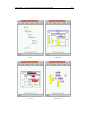
A survey in Personal Computer World [76] reviews the leading visual development tools for
the desktop market, where the leading platform is Microsoft Windows 95/NT. The products under review are Delphi 2.0, Optima++ 1.5, Power Objects, PowerBuilder 5.0, VisualAge Basic,
Visual Basic 4.0, Visual C++ 4.2, Visual FoxPro 5.0, Java Workshop, Visual J++, Visual InterDev, Visual Basic 5.0, C++ Builder and Visual Café. Most offer database connectivity, object
orientation, application builders, visual design, visual navigation and embedded help systems.
The programming languages Java, C++, Pascal, FoxPro and Basic are used. Visual aspects of
these systems include
A graphical user interface.
A windowed environment.
Dialog boxes, tool-bars and pull-down menus.
What-you-see-is-what-you-get (WYSIWYG) form designers.
WYSIWYG graphical user interface design (menus, dialog boxes and graphical resources).
Visual browsing of program resources (including graphical resources and program libraries).
Code navigation using visual browsers of procedures and classes.
Code navigation between code and GUI events.
Visual modification of the properties of some types of program object and resources.
Dialog box based skeleton code creation for components and applications.
There are only three visual notations used, each supporting interaction:
Direct representation (of graphical resources, forms, menus, dialog boxes and source
code).
CHAPTER 2. PREVIOUS WORK
23
Nested list representation for hierarchical structures (such as procedures, classes, methods,
help and graphical resources).
Table or dialog box representation for program object properties.
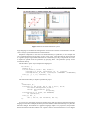
Here we see a success of visual languages in designing spatial things (graphical user interfaces) spatially. These products do not however provide visual support for the programming
itself, and merely insert code templates which the programmers need to flesh out themselves.
While clearly useful, there are only a very limited number of application views, using only the
nested list notation and are used just for code navigation. But even these techniques offer greater
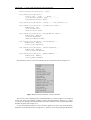
ease in building large high quality applications. Figure 2.4 shows a screen shot of Microsoft
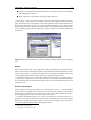
Visual Basic.
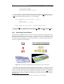
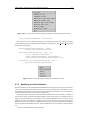
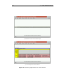
Figure 2.4. Microsoft Visual Basic 5.0, showing dialog box design and the project navigation
tree.
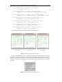
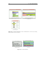
Genitor
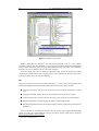
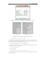
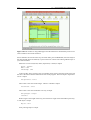
Genitor (from Genitor Corp. 1 ) goes further than ordinary development environments because it
offers a suite of tools for automatic navigation, project management and documentation. Its class
editor, shown in Figure 2.5, provides a navigation tree that visualizes the method structure, and
can be manipulated (via menus and drag and drop) to change the program objects.
While Genitor has access to a great deal of data about the program, its graphical output is
very limited. A navigation tree shows only the structure of the file, and other interrelationships
are not illustrated, but accessed through navigation. Its views are hard coded using just lists and
a nested list view.
Source Code Analyzers
Source Navigator (from Cygnus Software 2 ) is a development tool for C++, Java and COBOL
that provides tree and graph views of the system. It shows the class hierarchy, cross references
between classes, symbols used in the source code in a tree, and a graph of header file inclusion.
It can manage projects in excess of 100 000 lines of source code.
CC Rider (from Western Wares3 ) uses a source code analyzer to view the structure of C++
programs. It can show class hierarchies, class ancestries, function call trees, class nesting, header
file inclusion, symbols and program statistics. It can be used to navigate to parts of the source
code, and provide detailed information about program objects.
1 URL:
http://www.genitor.com
http://www.cygnus.com
3 URL: http://www.westernwares.com
2 URL:
24
2.4. SOFTWARE VISUALIZATION SYSTEMS
Figure 2.5. Genitor’s class editor.
SNiFF+ (from Take Five Software 4 ) has source code analyzers for C, C++, Java, Fortran,
Assembler, Python, Tcl, Perl and Bash. It provides project and documentation management,
views of class hierarchies, class browsing and include browsing, and source code navigation.
Projects in excess of a million lines of code can be analyzed.
In these systems, the views are fixed, the information they provide is limited, their output
vocabulary is limited, and they have no support for run-time information. However they offer a
great improvement over text-only programming.
Tau
Tau [70] is a collection of tools to navigate and profile C++ source code, and incorporates class
browsing and displays detailed run-time profile information visually. Views include
File and class display. This provides list boxes to browse methods and classes in source
code.
Call graph extended display. Shows the calls made between functions as a graph.
Class hierarchy browser. Shows the class hierarchy, and a window lists class members.
Routine and data access profile display. Displays run-time usage of data.
Speedup and parallel execution extrapolation display. Shows graphs of the performance of
parallel C++.
Tau’s visualization is too limited to classify it as a SV system. Tau is implemented manually
- there is no easy way of extending the views or the system, and its output form is limited to
numerical graphs and a class hierarchy.
4 URL:
http://www.takefive.com
CHAPTER 2. PREVIOUS WORK
2.4.2
25
Visual Programming Systems
Visual programming systems consist of a visual editor to construct visual programs in a visual
programming language, and a means of executing the visual programs. In Price et al.’s definition
[79], SV encompasses VP because VP is a specialization of SV that allows interactive modification of the program. VP systems use many visual programming languages (VPLs), visual
representations of software, and techniques to interact with visualizations to modify the program.
Visual programming languages have existed since 1966 [99], and there are now hundreds of
VPLs in existence. VPLs are becoming as prolific as textual languages, although there is not the
same tool support (such as Lex and Yacc [2]) for visual programming [36], making it considerably more difficult to implement visual programming languages than a textual ones [71], and only
a small number are commercially viable. VPLs that have had particular commercial importance
include LabVIEW [104], ProGraph [19, 77], VisualAge (from IBM), Visual AppBuilder (from
Novell), AVS (from Advanced Visual Systems) and AppWare (from Novell). Visual languages
are more successful as end user languages for specific applications than as general purpose programming tools.
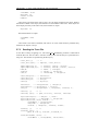
Figure 2.6. The quicksort algorithm written in ProGraph.
ProGraph, originally described by Pietryowski [77], is one of the most successful and widely
used VPLs. Figure 2.6 shows an example of a ProGraph program.
It is plausible to suggest that visual languages might one day supersede the textual programming paradigm. At present practical issues such as scalability [17] and tools [36, 65, 71] need to
be solved to make visual programming a viable alternative to textual programming.
2.4.3
Code Visualization Systems
Code visualization provides graphical information about the source code of a program. It includes high level overviews, program structure, and source code itself. It is different to visual
programming in that code visualization systems do not necessarily modify graphical representations of code.
SEE
SEE [4] is a source code pretty printer that goes much further than syntax colouring. Syntax
colouring is often used in text editors which identify the lexemes present in the source text and
colour them according to their type (for example reserved words or comments). Syntax colouring
gives demonstrable benefits to programmers, resulting in fewer syntax and typing errors, and
faster comprehension of the source code [4].
SEE converts source code into the style of a technical manual for automatic documentation.
Type-faces, bold and italic emphasis, font size and shading are used to display the source text,
26
2.4. SOFTWARE VISUALIZATION SYSTEMS
with one procedure per page, and procedure parameters clearly laid out in a table. Cross references to other procedures are generated automatically. There are other source formatting utilities
available, including vgrind (in BSD Unix) and WEB (part of the TEX typesetting system).
SEE is very limited in its output - its output format is fixed, and it does not make extensive
use of graphics.
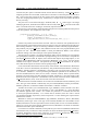
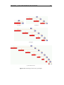
SeeSoft and SeeSys
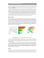
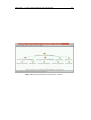
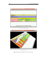
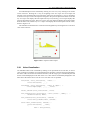
SeeSoft [29] by AT&T Bell Labs is a SV system that produces line-oriented software statistics
of the source code in a software project. Each line of source code is represented by a single horizontal bar, contained in a vertical bar representing each source file. Modification statistics are
compiled for each line of source code, which are then displayed using a coloured scale (continuous or discrete) showing update frequency, or time of last update. Files can be grouped according
to function, and Figure 2.7(a) shows the screen layout.
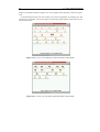
(a) SeeSoft.
(b) SeeSys.
Figure 2.7. Line oriented software statistics.
The display is interactive, allowing users to drag small windows over each source file to display actual source code, and change the colour scale. This visualization technique is sometimes
referred to as a mural [49], where a long display is compressed in one dimension so that it may
be contained within the screen, and a superimposed slider then magnifies the region of interest.
Murals obey Shneiderman’s “visual information seeking mantra: overview first, zoom and filter,
then details-on-demand.” [91]
Baker and Eick [5] attempt to solve the problem of screen size and scalability by developing a system called SeeSys to visualize software systems using line-oriented software statistics.
Instead of using fixed width bars with lengths proportional to the number of lines of code, the
screen is divided into rectangular regions as shown in Figure 2.7(b) with rectangle areas proportional to the lines of code. The system can visualize files, directories and subsystems, and there
is a zoom facility to zoom in on any subsystem. Additional information is presented to the user
as the mouse moves over the visualization.
The output of SeeSoft and SeeSys is inflexible, so that the output data and format it fixed.
There is also only one type of information available: the modification history of each line of
source code, and the size and modification history of each source file. Nevertheless they provide
a useful browsing and overview facility.
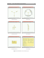
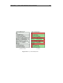
Graph Visualizer 3D
Graph Visualizer 3D (GV3D) [32, 105] is a tool to create three-dimensional visualizations of
networks, and in particular of computer software and object-oriented code. Figure 2.8 shows
CHAPTER 2. PREVIOUS WORK
27
visualizations it can produce. By itself, GV3D is just a graphical output library that can be
interfaced to analysis tools.
(a) Calls.
(b) Class hierarchy.
(c) Modules.
Figure 2.8. Renderings of almost 6 million lines of code by Graph Visualizer 3D.
2.4.4
Algorithm Animation Systems
Algorithm animation systems illustrate the principles of an algorithm by illustrating its operations
on a data structure. Sometimes the animations don’t relate to a real program at all, but are simply
animation scripts. Of special interest is how the underlying program is connected to the output
graphics, which is often no more complicated than embedded calls to a specialized graphics
library.
Tango and Polka
Tango [95] is an algorithm animation system by J. Stasko at the Georgia Institute of Technology
that can create smooth animations using smooth path transitions between execution steps. Animations are designed using trajectories and changes in size, colour and visibility. The source
code is annotated to generate abstract data events, and under execution the data events map to
animation events to generate the animation. Animation calls and visualization setup are written
in C and inserted into the source program. There are user controls to pause, control speed and
pan the display, and the visualizations are 2 and 2 21 dimensional, animated in real time. Figure
2.9(a) shows XTango - Tango for X-Windows that visualizes animation scripts generated from a
running program.
(a) Bin packing in
XTango.
(b) Minimum spanning subtree in Polka.
(c) Quicksort in
Polka-3D.
Figure 2.9. Visualizations produced by Tango and its derivatives.
Tango has now been superseded by Polka [96], which is well suited for colourful smooth
animations of parallel programs. Animation calls are made from a running algorithm that call a
28
2.4. SOFTWARE VISUALIZATION SYSTEMS
C++ library to effect animation events in a display. Objects are created that can be moved around
the scene. Samba is a front end to Polka that accepts animation directives from a text file. Polka
supports 2-D and 2 21 -D visualizations, shown in Figure 2.9(b), but Polka-3D produces full 3-D
visualizations shown in (c).
Several visualization systems have been built upon Polka, including PARADE [97] to visualize parallel and distributed systems, ConchViz to visualize the execution of cluster and messagepassing environments. PVaniM visualizes and animates data from a Parallel Virtual Machine,
which sends communication and user event statistics back to a monitor for visualization. There
are other visualizers for parallel processes, including XPVM, Xab, PVMTrace and Pablo [57].
The main drawback with Polka is that it offers little more than an animation library in C++.
Because the animator must manually write all of the animation calls, it is very time consuming
to create animations in Polka. A degree of expertise is required to learn the library.
Balsa and Zeus
Zeus [15] by DEC SRC is written in Modula-3, and is based upon an algorithm animation system called Balsa [16]. Balsa itself was used as a teaching aid for algorithms using algorithm
animation, and provided a windowed graphical display, panning, zooming and allowed users to
view the execution of several algorithms running simultaneously, and can provide synchronized
multiple views of the same algorithm. The user is able to set the graphical display of data items,
and a source window with pretty-printed text is also available. Balsa works by inserting interesting event points into the source code (also known as annotating the source code), which generate
visualization scripts that can be replayed.
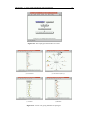
(a)
(b)
(c)
Figure 2.10. Output from the Zeus algorithm animation system.
Zeus supports synchronized multiple configurable views. Zeus can run in a multi-threaded,
multi-processor environment, making it suitable for visualizing parallel programs, some sound
extensions have been incorporated into Zeus, and Zeus now supports 3-D. Figure 2.10 shows
Zeus in operation.
Zeus uses Modula-3’s class hierarchy to define views of an algorithm. Each running algorithm
generates animation events, which call the animation library to provide output to the user. The
effort of setting up new animations is high because the algorithm must be implemented within
the Zeus framework, and hence does not correspond to real-world programs. The programmer
must manually insert calls to Balsa and Zeus to perform the animation actions, requiring a priori
detailed knowledge of the algorithm.
Pavane
Pavane [84, 86] is a visualization system that is capable of visualizing the run-time behaviour of
parallel and massively parallel architectures. Parallel, distributed and concurrent execution is a
very common subject of visualization because concurrent execution is so difficult to understand.
CHAPTER 2. PREVIOUS WORK
29
The implementation consists of five modules that can be distributed across a network, providing a parser to an intermediate language, a run-time execution monitor, visualization utilities,
a renderer and a viewer. This architecture allows remote and distributed visualization. Visualizations in Pavane are specified in a declarative style [85], where a mapping is defined between
the data space and objects in the visual space. This gives a powerful degree of abstraction of the
visualization from the data. Smooth animation can also be defined. Its output is shown in Figure
2.11.
Figure 2.11. An animation of sorting by Pavane.
Pavane visualizations are very complicated to set up. The target program in C is manually
annotated by inserting a number of calls that initialize Pavane and declare the data to watch
(via the VisualMonitor() function). Event points are inserted into the source code by calling
VisualUpdate() which tells Pavane to update the visualization with the new state.
A file containing visualization rules declares how to produce the visualization. Only numerical values and arrays can be passed to these rules. Each rule declares objects in the scene, and
their screen coordinates depend on the values obtained from the C state. Expressions map the
input data to coordinates in the scene. The syntax of these visualization rules is very complex.
Once the system has been set up, quite powerful visualizations are possible.
The main problem with Pavane is the manual effort and complexity in defining new visualizations. Its specification language is very cumbersome and low level.
Leonardo
Leonardo [20] is an algorithm animation system that provides a logic programming language
called Alpha to define graphics corresponding to data of a program executing in a virtual machine.
Leonardo claims to be much easier to use than Pavane [85], and its virtual machine can be stepped
forwards as well as backwards. An output from Leonardo is shown in Figure 2.12.
Declarations in Alpha are embedded in the object program within /** and **/, for example
int g[MAX_NODES][MAX_NODES];
/**
Graph(Out 1);
Node(Out N, 1) For InRange(N, 0, gNumNodes-1);
Arc(X,Y,1) If g[X][Y]==1;
**/
Alpha declarations are simply logical predicates. It is similar to Prolog, but has a much more
awkward syntax and has to define parameters as either inputs or outputs, and lacks unification
and compound terms. Variables can only be integer types. Expressions from the target language
can be embedded into Alpha directly. Whenever an Alpha predicate is called, expressions in the
30
2.4. SOFTWARE VISUALIZATION SYSTEMS
Figure 2.12. The Leonardo animation system.
target language are evaluated according the the current state of the the virtual machine. Thus the
view is always synchronized with the virtual machine.
Graphical components in the scene are declared directly as predicates, so for example the
Arc/3 predicate declares the presence of arcs in the scene. This approach has been proposed
as a general purpose logic-based framework for visualization [23, 24]. Components of a scene
in Alpha are “pulled” from the predicates by querying them. The predicates specify screen
coordinates directly.
The alternative “push” style of imperative languages is
void draw() {
Window(_W);
for(int RecID=0; RecID < num; RecID++)
Rectangle(_W, RecID, 10+RecID*20, 10, 15, a[RecID]),
RectangleColor(_W, RecID, a[RecID]<50 ? DARKGREY : LIGHTGREY);
Line(_W, _L, 5, 10, 10+num*20, 10);
}
The same functionality in Alpha is specified in [23] as
/**
Window(Out _W);
Rectangle(_W, Out RecID, Out X, Out Y, Out L, Out H)
For RecID:InRange(RecID,0,num-1)
Assign X=10+RecID*20 Y=10
L=15
H=a[RecID];
RectangleColor(_W, RecID, Out DARKGREY)
If a[RecID]<50;
Line(_W, Out _L,
Out 5, Out 10, Out 10+num*20, Out 10);
**/
As can be seen, the Alpha program is actually longer and more obscure than the imperative
language! In the above example, the draw() function could be called automatically every time the
data state changes. Nevertheless as a graphics language, Alpha is very expressive, and provides
abstraction between the data and the view. Alpha is still low level because there is a low degree
CHAPTER 2. PREVIOUS WORK
31
of abstraction between the output of Alpha and the graphics on the screen. The Alpha script must
be reprogrammed to change the output.
Eliot
Eliot [61] extends Polka [96] to make it automatic to use. Algorithms written in C are compiled
in C++ to overload the C operators to invoke visualization events. For example, each type of
program object such as an array or integer, is created as an Eliot class, and any attempt to make
assignments to the data calls the overloaded operator which updates the display. The user can
choose the graphical representation of the run time data from a menu, and display different
outputs in different windows.
Eliot is much simpler to use than any of the other systems in this section because it is completely automatic, and the user’s intervention with the source code is minimal. It also has much
greater potential for intelligence, and can be used in conjunction with the standard Polka calls.
Unfortunately Eliot still requires some modification of the source code, and its output is not as
flexible as animation systems that program their animation explicitly. Eliot can only visualize
integers, reals, characters, arrays and binary trees. Visualizing other structures would require
special implementation. Eliot can only show the current data state.
2.4.5
Run-time Visualization Systems
Run-time visualization displays what is happening in a program as it is running. This can monitor
code (including program statements, threads or object usage), and data. Data visualization differs
from algorithm animation in its purpose and degree of abstraction. Data visualization reveals
real data in running systems for analysis, while algorithm animation is mainly used for teaching.
Algorithms and algorithm animation are more abstracted from the underlying program.
The University of Washington Program Illustrator
The University of Washington Program Illustrator (UWPI) [42] offers a source level run-time
debugger of Pascal programs (allowing single instruction steps in the source code) that provides
an automatic visualization of the data in the program. A layout strategist written in Lisp applies
AI techniques to determine the best way to render the program data, and displays the current data
state graphically in a window.
According to Price et al. [79], “UWPI is the best example to date of automatic SV with any
kind of intelligence.” But UWPI can only illustrate small programs involving sorting and graphs,
and only possesses a shallow understanding of numerical program data.
GROOVE
GROOVE [89], from the Georgia Institute of Technology, illustrates the run-time behaviour of
object-oriented systems using animation, so that programmers can better understand the class
hierarchy and relationships. Figure 2.13 shows GROOVE.
GROOVE animations are created by manually creating visual objects in the scene from function calls. Therefore while GROOVE is flexible in its output, there is a degree of effort to create
visualizations, and the system is only suitable for small programs.
Look!
Look! (from Objective Software Technology 5) is a commercial product that allows visual display
of the run-time behaviour of C++ systems. It is claimed that this allows programmers to understand the system much more quickly, find bugs much faster, reduce redundant object behaviour,
and improve the overall code quality. Programmers can view references between classes, the
5 URL:
http://www.objectivesoft.com
32
2.4. SOFTWARE VISUALIZATION SYSTEMS
Figure 2.13. Screen-shot of GROOVE showing an object-oriented design.
class hierarchy, object creation and deletion events and concurrent threads. Each view shows the
current method acting on the objects.
Look! views are hard coded, and actually provide just four different visualizations: class
references, class hierarchy, object creation and code clustering. While the system is automatic, it
is dedicated to just these views and cannot be extended by the user. The views themselves show
only object names and method invocations.
2.4.6
Architectures
Viz
Viz [26, 27] is a framework developed at Open University in which run-time SV systems may be
built. Viz uses players, which can be any program object such as a variable, a function or a code
block, to generate history events, shown in Figure 2.14(a).
(a) Acquiring and filtering history data.
(b) The architecture of Viz.
Figure 2.14. Viz.
The system architecture is shown in Figure 2.14(b), and consists of histories, views (individual
visualization windows), mappings (translation from view information into graphical output) and
navigators (to manipulate and move between views).
CHAPTER 2. PREVIOUS WORK
33
Viz itself provides only a framework for implementation, and does not provide a specification
language.
Vogue
Vogue [51] is a 3-D visualization system that has been applied to parallel/concurrent programming, object orientation and software engineering. Systems built using Vogue include VisuaLinda [55], Integrating Version Control and Module Management [54], Fractal Views [52, 56]
and Bottom-up Program Visualization [53].
Vogue’s primary operation is to extrude an array of 2-D networks into a 3-D image. The
argument is made that more information can be fitted onto the screen, and the evolution of a
system can be viewed in a static diagram. However Vogue is an architecture that provides only
nodes and links that must be created manually in the source code. Its output capabilities are very
limited, using just colour, shapes and lines to communicate information. Vogue is actually just
an output library, and is not an end user system because a considerable programming effort is
required to generate visualizations.
2.5
2.5.1
Specification
Visual Language Theory
Visual language theory [65] explores formalisms for structuring the visual domain, and how
graphical structure relates to the semantics of visual languages. From a theoretical standpoint,
a visual language is “a set of diagrams which are valid ‘sentences’ in that language, where a
diagram is a collection of ‘symbols’ in a two or three dimensional space.” [65] One of the main
issues in visual language theory is defining membership of visual languages. The main methods for specifying visual languages are graph grammars, attributed multiset grammars, logical
formalisms and algebraic formalisms.
The main drawback with visual language theory is that it deals with interpretation, not view
generation. This is useless for visualization, where the task is to generate the diagram in the first
place. One grammar that is generative is given by Grant [36], where the grammar defines the
geometric transformations of objects that are contained in one another.
In its broadest sense, parsing images is a vision problem. In visual language theory, diagrams
are used where the symbolic constituents of the diagram are known. Such a pre-processing stage
is analogous to lexical analysis. Parsing diagrams is more costly than parsing text, because of
the unordered nature of the constituents of a diagram, and because geometric conditions must be
tested.
Visual Grammars
The two main types of grammar are graph grammars and attributed multiset grammars. Graph
grammars [81] regard the view as a set of interconnected symbols. Graphical rewrite rules specified in the grammar transform the graph of the image structure.
Attributed multiset grammars consist of rewrite rules on collections of symbols with attributes.
One of the most general and powerful types of attributed multiset grammar are Constraint Multiset Grammars [65]. Geometric constraints on the attributes are tagged to the grammar rules.
Such grammars can be implemented in Prolog, by using constraint logic programming [48] to
specify the geometric constraints.
Semantics of Diagrams
The semantics of diagrams can be described by logical or algebraic formalisms. As well as using
logic to reason about geometry, description logics [28] can be used to assign meaning to the
34
2.6. INFORMATION VISUALIZATION
structure of the diagram. Description logics are less powerful than full first order logic, and are
therefore more tractable.
Algebraic specification [103] maps the application domain into typed abstract data structures.
An image is mapped into a data type, representing concepts or semantics. Algebraic rules define
a functional mappings between the domains.
2.5.2
Numerical Data
Numerical data has particular significance in scientific visualization, and has uses in software
visualization. Numerical-only methods are insufficient for heterogeneous visualization and visual languages. Hibbard et al. [43] develop a scalar mapping technique for mapping numerical
data in a program to continuous quantities in a display, including time. A system called VISAD implements a specification language that defines data structures (of numbers), and mappings
between elements in the data structures to graphical display coordinates. For example
map earth_location to xz_plane;
map temperature to y_axis;
In later work by Hibbard et al. [44], a lattice model describes the relationship between data and
display. They concede that their technique is “inadequate for complex information processing”
such as recursive data structures, and they foresee “considerable technical difficulties” to manage
such data.
2.5.3
Specification Languages for SV
SV systems fall into three categories: those that are not extensible at all, those which are extended
in the native programming language, and those that provide their own language for specification.
Only Pavane, Leonardo, VIS-AD and Samba fall into the last category. Samba is merely a
sequence of visualization and animation directives.
Both Pavane and Leonardo use a declarative specification to map live run-time data to graphical objects. The drawback with both systems is that they only provide a direct mapping to
graphical objects on the screen. Thus they are both very low level approaches. Another problem they have is that they lack encapsulation, for example to define libraries of objects, and the
mapping from the data to the graphics is fixed. A change in the mapping can require significant
reprogramming. The implementations of Pavane and Leonardo are very different however.
VIS-AD also provides a declarative specification for mapping data to the screen, but is restricted to simple numerical data structures.
In spite of their limited success, declarative specification languages offer significant advantages over imperative programming methods [20]. For example they offer a higher degree of
abstraction between the data and the graphics, the languages are specialized to the task, and are
potentially easier to use.
2.6
Information Visualization
The wider field of information visualization looks at techniques for expressing all types of information in a visual form. Visualization has proved an extremely important use of computers,
where the information they store needs to be output, and often visualization communicates information far more effectively that textual data. Visualization has applications in virtually every
field, including business, science, finance, management, databases, information retrieval and
software engineering.
CHAPTER 2. PREVIOUS WORK
2.6.1
35
Perception
The study of visualization examines what information to visualize, what visual representations
to use (i.e. what visual languages to use), and how the visualization is created. The study of
choosing visual representation lies largely in psychology, which regards visualization as a mental
process, and performs experiments on human subjects to find metrics for human responses and
the effectiveness of various types of notation. Creating the visualization is essentially the problem
of computer graphics, and includes rendering, graph drawing and spatial constraint solving.
Psychological factors are rarely applied to SV, mainly because it of the absence of techniques
to empirically measure the effectiveness of SV systems [79]. This does pose problems for objective and meaningful comparison between systems. Much of the SV literature completely disregards psychological factors, and merely regards visualization as a conversion from a program
to a graphical representation, for example [84]. Psychological experiments must be performed
under very controlled conditions, and software visualization is too large a domain to measure
directly. The result is that psychology has so far offered few concrete ideas to SV that could not
be derived using intuition, and indeed visualizations and visual languages can, and generally are,
devised on an ad hoc basis, and are only informally evaluated.
There are psychology studies that can contribute to creating more effective visualizations.
Rogowitz et al. [82] look at how we can exploit preattentive perception and colour/luminance
mappings to create visualizations that can be searched more quickly and convey continuous or
discreet data with greater veridicality. Perceived brightness is proportional to a power of luminance (hence gamma correction), so where luminance is used to convey continuous data, a
corrective power should be applied, and examine other stimuli for conveying continuous information. Perceived colour varies discretely with hue (wavelength), so this should be exploited for
discrete data, but compensated for in continuous data. Experiments in preattentive vision show
how we can subconsciously pick out certain features of images (e.g. coloured spots), which can
be exploited when searching large datasets in constant time, versus a linear searching time for
attentive (conscious) searching. Preattentive effects can also disrupt the interpretation process by
distracting the subject from the important features, and should be exploited to attract or direct
attention to the important features of the visualization quickly.
Rogowitz and Treinish [83] propose a visualization system that considers perceptual rules
to devise a visual representation for data. They argue that this is required because traditional
visualizers may introduce unwanted artefacts into the image that obfuscate the meaning of the
visualization, as described in [82]. They also claim that visualization is easier to implement
and produces better and more meaningful representations when visualization rules (based upon
perception) are used to generate visualizations, than high-level tools or direct coding. Current
SV systems use high level tools and direct coding, which produce inflexible visualizations and
offer little guidance on the effectiveness of the visualization.
2.6.2
Representations
Some systems use a three dimensional representation. There are advantages in using the third
dimension, including added realism and tangibility of program objects, increased information
density, and an extra quantitative axis. Shneiderman [90] argues that programmers think of their
code as structural and tangible, and that direct manipulation of abstract objects in the computer
using a visual paradigm would be the easiest and most natural way to interact with a computer.
The 3-D approach adds reality and tangibility to the program objects, thus concretizing the software more effectively for the programmer. However there is evidence that making objects more
realistic makes it more difficult for users to extract the information (or abstract the semantics) that
the symbol conveys [63]. There is also evidence that 3-D visualizations can convey between “1.6
and 3.0” times more information than an equivalent 2-D view, and users are able to understand
complex relationships better when presented in 3-D [105].
Lohse et al. [63] derive a classification of various basic types of visual representation, by asking subjects to sort a set of sixty images of a full range of visual representations. By performing
statistical tests they compiled a taxonomy to grade each of the images according to the high level
36
2.7. RESEARCH DIRECTIONS
properties of spatiality, temporality, comprehensibility, level of abstraction, continuity, attractiveness, subdivision, numerical level, dynamic vs. static and information rich vs. information
poor. It emerged that there are eleven major clusters of representations: graphs, tables, graphical
tables, time charts, networks, structure diagrams, process diagrams, maps, cartograms, icons and
pictures. The work offers many ideas and visual representations - or combinations of them - that
could be applied to SV, and gives the principle characteristics of each representation.
Tufte [101] details methods for scientific visualization of quantitative information. He gives
a comprehensive collection of hundreds of graphical representations, with critique. This book
offers a rich source of ideas and much more useful rule-of-thumb approaches for effective visualization than attempting to rationalize visualization on a formal basis. Many visualizations of
software are quantitative.
Bertin [9] wrote one of the first texts on the semiotics or meaning of graphical representations.
This is an informal treatment of diagrams. Bertin regards “order, form and proportion” to be the
building blocks of any graphical representation. Bertin mainly considers visualizing numerical
tables. Green and Benyon [38] regard “entities, attributes and relationships” as the fundamental components of information display, and discuss, again informally, the relationship between
graphical properties (graphical artefacts), and the semantic properties (information artefacts)
conveyed by the display.
2.6.3
Architectures
The AVE system [34] implements a flexible mapping from data to diagram using a data-driven
approach, where the data itself determines how it is to be visualized, and AVE is particularly
applicable to semantic networks [28] where the database contains heterogeneous data. The data
relations are mapped onto graphical relations on the screen, such as interconnection or adjacency,
by analyzing the structure of the data. Queries select subgraphs of the database, which are subject
to structural analysis. Graphical relations are then assigned to the data relations using a ranking
system, and the diagram is generated to render the data with the assigned graphical structure.
Figure 2.15(a) shows the graphical representations it chooses for the various data structures, and
Figure 2.15(b) shows the overall architecture.
The drawback with AVE is that the ranking system is hard coded and it has only a limited
number of different layout techniques to apply.
2.6.4
Graphical Layout
Graph layout remains a difficult area of computer science. It is well known that optimizing
graph layouts is generally NP-hard, and in particular minimizing edge crossings is NP-complete
[33], so much work has been done in developing heuristics for graph drawing. Graph drawing
is an important tool for SV, where relational data may be presented in a node-and-link fashion.
There are many ways to present graphs, including using polylines, straight lines, as orthogonal
drawings, as rooted trees, as free trees, in planar form, in 3-D, as convex, as gridded, as directed,
as undirected, as hierarchical etcetera. A comprehensive survey of graph theory and methods is
given by Battista et al. [6]
2.7
Research Directions
Both Myers [71] and Price et al. [79] identify several deficiencies in current systems that should
be addressed in future research. The reason SV systems are not more successfully applied is
because of these difficulties.
Both Price et al. and Myers say that formal specification of SV and VP systems is limited, and
although theoretical work has been done in visual languages, it has so far proved to be impractical
for SV.
Without the foundations for specification, and without formal data representation, it is difficult
to provide specification for scripting. Scripting facilities for SV systems are extremely low level,
CHAPTER 2. PREVIOUS WORK
37
(a) Mapping data to graphical structure.
abstract visualization
query
analysis
constraint
network
generation
geometric
layout
(b) Architecture (reproduced from [34]).
Figure 2.15. The AVE visualization system.
often consisting of in-line C code, and the data representation and management is usually ad hoc.
This means that it is cumbersome to add views to systems, so SV systems tend to have a very
limited number of views. The lack of views leads to fixed granularity, poor elision control, and
poor or no navigation. Work is therefore needed to make SV easier to specify and implement.
The comparative difficulty of specification extends to layout, interaction (if possible at all),
and navigation which are all manually coded. It makes it more difficult to change the graphical
representation once the view has been implemented. Intelligence and flexibility are required,
because a representation that is appropriate for 10 elements is unlikely to be appropriate for
100 000. AVE [34] and Rogowitz and Treinish [83] suggest ways to correct this. Work is needed
to improve the tailorability and flexibility of SV systems.
It can be very time consuming to set up visualizations and add new views, to the point where
the cost of setting up the view outweighs the insight gained from the visualization, particularly if
the insight is difficult to gain because the data is represented inappropriately. Standard empirical
evaluation methods for SV do not exist because the programming task is difficult to quantify.
Hence evidence of worth is lacking for many SV systems. SV systems must be made easier and
more automatic to use.
Scaling up systems to tackle large applications is a problem for many systems, caused by
lack of proper data management to handle large data sets effectively, poor view granularity, poor
elision control, poor automation, and poor flexibility in graphical representation. Hence most of
the visualization systems presented here only display small quantities of data. Work is needed to
manage large data sets and control elision more effectively.
2.8
Conclusions
Software visualization is an emerging field, and is becoming increasingly important in understanding, documenting, debugging and constructing software. The great success of visual tech-
38
2.8. CONCLUSIONS
niques in professional development tools has greatly cut application development time and improved application quality, and is set to continue as more techniques move from experimental
systems into commercial ones. As software complexity grows, more powerful techniques must
be devised to maintain large software systems.
The trend is that software development is becoming more visual, although visual programming languages are still inadequate to replace text entirely in most circumstances. Like visual
programming languages, software visualization systems must demonstrate their benefits before
they will gain widespread acceptance. Work must be done to find applicable formalisms for both
visual languages and software visualization to allow progress. Software visualization is currently
impeded by lack of high level specification, which could provide solutions for many problems,
including view specification, quantity of views, graphical mapping flexibility, granularity, elision
control, navigation, scalability and automation.
Chapter 3
A Model of Information
Visualization
Software visualization presents unique challenges because the data presented is so
heterogeneous and the graphical output can be so varied. What kind of theory could
underlie such an open ended task? Current theories of visualization or visual languages do not adequately model the semantics of graphics, or are too limited, so
existing implementations are not based on formal approaches.
The work in this chapter presents such a theoretical model that formally models
the relationship between graphics and its semantics. It is named a semantic model
because in this model, the semantics of graphical views are always explicit. This
in turn leads to a decoupling of the information content in a view, and its graphical
representation, and allows arbitrary queries to determine the content of a view.
An important aspect of any theory is its applicability, and the purpose of this theory
is to provide an extremely concise and high level specification method. This will be
used as the core of a visualization engine that is described in Chapter 4. Chapter 5
applies these specification techniques to software visualization.
3.1
Introduction
Software visualization is laborious to implement because the current tools are not sufficiently
automatic and flexible, and lack effective scripting [79]. Computer software contains very relational, structured and heterogeneous data, and visualization tools are ill-equipped to manipulate
this kind of data because theory on visualization and has not been fully developed to handle
arbitrary data structures.
In this chapter a theory of visualization is developed that forms the basis of a generic visualization tool that will be used to visualize software. Foundations are a necessary first step,
and provide a common language, a framework for implementation, and the capability for formal
reasoning.
While there are many automatic tools for numerical and scientific visualization, heterogeneous data visualization has proved to be much more difficult to model and specify [44]. Existing
approaches to heterogeneous data visualization rely on low level programming using imperative
languages. Even declarative specification approaches such as Pavane [86] and Leonardo [20]
explicitly specify graphical positions on the screen, and deal only with numerical quantities. The
benefits of declarative or logic specification languages are not fully realized when such a low
level approach is used, and logic languages such as Prolog are inferior to imperative languages
for implementing general graphical algorithms because of their slow speed and lack of efficient
data structures.
In this chapter these basic declarative approaches are improved. Instead of directly mapping
39
40
3.1. INTRODUCTION
numerical data to screen coordinates, the visualization process is further subdivided as shown in
Figure 3.1.
Flexible mappings
01111010101
01010100001
10101001100
11111000000
sample(9,125)
age(harry,15)
woman(diana)
won(player1)
person(harry)
person(diana)
mother(diana,..
father(charles,
line(di,harry)
label(harry,15)
title(Title)
Input
Data
Source
View
Content
Visual
Content
Title
Graphical
Constraints
Title
Output
Image
Figure 3.1. A semantic model of visualization.
The output is generated from a set of graphical constraints, which include spatial associations
such as adjacency, containment or connections, attributes such as colours, and objects such as
polygons and text. This is a much more high level approach to specification, and is completely
generic.
Deriving the graphical constraints for a view is split into several steps. The first step is data
gathering from the input shown in Figure 3.1, to provide a data source in some database. The
information content in a view, or view content, is acquired by issuing a query to the database
to construct a set of data. A one-to-one mapping maps the information content to a graphical
representation, or visual content. A third mapping defines the graphical constraints that compose
each visual in the visual content. We define a visual to be a set of graphical constraints that
represents some meaningful graphical notation.
There are many advantages with this approach:
Screen coordinates do not need to be specified, but are derived automatically by layout
algorithms. Previous systems have only provided direct mapping to the display, and are
therefore less flexible in their graphical output.
It is possible to change the mapping from view content to visual content without redefining
the views. It also makes it possible to provide multiple graphical representations for the
same data. Previous systems have only provided a fixed mapping, which must be edited in
text to change the view.
These mappings can be fully formalized, and embedded in first order logic. It is possible to reason about heterogeneous data visualization. Previous systems do not base their
specification on a formal model of visualization.
These mappings can be specified straightforwardly in Prolog. This means that there is no
need to devise a new language, and is therefore much easier to implement and will run
much faster.
Because Prolog is introspective (it can query its own program) and dynamic (it can modify
itself), these mappings can be queried and modified by the user at run time. Other systems
offer fixed visualization behaviour, and cannot display an automatic legend describing the
view. The fact that the mapping between view content and visual content is a bijection
permits this.
It is possible to pose arbitrary queries to a knowledge database. Previous systems restrict
this to run-time data.
Visuals are specified independently of the view data, and can be reused. This is a big
problem for previous systems which effectively have to start from scratch each time a new
view is created.
Multiple views can be defined independently and used within the same system. By labeling each view and visualization mapping, directives such as “visualize function(Fn) using
coloured nassi shneiderman diagram” can be issued. Support for multiple view definitions in other systems is much more limited.
CHAPTER 3. A MODEL OF INFORMATION VISUALIZATION
41
Arbitrary data structures can be passed through the visualization pipeline. Previous systems deal only with numbers, which is too limited.
It is possible to interact with objects in the view, because they are assigned identifiers of
objects in the database. Interaction is also specified formally. It isn’t possible to specify
interaction in other declarative systems.
3.2
Representing Data
Data gathering is an essential first step in any visualization system. Therefore it is necessary
to formalize the notion of the data from which to visualize. Previous approaches [23, 44, 86]
restrict this domain to numbers - this domain must be extended to encompass all types of data.
The approach we shall use is to regard this data as a set of propositions that can be computed
to be true. Such a notion has little meaning in an imperative language, but in logic programming
it is the set of propositions that can be proven from the inference rules of the logic program. The
canonical form of logic programming is the programming language Prolog, although there are
many other logic programming languages. We shall restrict ourselves to the core language.
Using Prolog has several advantages for data representation. First of all it is a very high
level language for expressing relationships and inferences between data, and can express high
level rules very naturally. Prolog is a good meta-language, so it is suitable for representing
and reasoning about computer languages which are entirely rule-based. The work described in
Chapter 5 shows that all aspects of computer languages can be modeled in Prolog.
A Prolog program constitutes a set of logical inferences in first order logic. 1 In other words
Prolog is itself a formal notation, which removes the need to develop further notation in this chapter. Formal treatment of Prolog and first order logic is well established and is treated elsewhere
[80].
A common application of Prolog is in knowledge engineering and automated reasoning [62].
Visualization has potential uses for displaying the results of automated reasoning, while automated reasoning adds flexibility to derive new knowledge (implicit knowledge) for presentation
in a visualization system. Information visualization is the presentation of knowledge, so it is
natural to integrate knowledge engineering into visualization.
Prolog is Turing powerful, so it can compute everything that a language such as C++ can,
although the language has different applications. Prolog can perform any perform any kind of
data manipulation. The following examples illustrate Prolog’s approach to data representation.
Example 1. Suppose sea-bed data is visualized, and at each discrete sample point lies the sea
depth and its temperature. The predicate
sea_depth(X, Y, Depth)
would convey the depth of the sea at the specified location, while
sea_temperature(X, Y, Temperature)
would convey the temperature at each location. Data would be added to these predicates from
an external source. A query such as
?- sea_depth(X, Y, D), D>10, D<12.
would return all locations where the depth was between 10 and 12 metres.
Example 2. Suppose wiring of a house is visualized. The predicate
socket(Socket)
1 Pure
Prolog implements first order logic. ISO Prolog [1] contains features such as cuts that can break the logic, but
are a practical necessity to prevent unwanted backtracking.
42
3.3. SPECIFYING VIEW CONTENT
would identify the sockets, while the predicate
location(Socket, Location)
would identify the location of each socket, perhaps by a description or a set of co-ordinates.
Wires could be indicated by
wire(Socket1, Socket2, Type)
to indicate the existence of the wires between sockets, with Type being live, neutral or earth.
Example 3. Suppose the liveness of variables was visualized over a function. Variables could
be represented as
variable(Variable)
and statements by
statement(Statement)
and liveness could be indicated by
live(Variable, Statement)
The query
?- live(V, s).
would return which variables were live for a particular statement s, while
?- live(v, S), live(V, S).
would return which variables are concurrently live with variable v.
3.3
Specifying View Content
When the data has been gathered it is ready to be viewed. A query is issued to the knowledge
database to extract the information to display. This is a set of terms called the view content,
which is shown in Figure 3.1. In this way, every datum in the view is represented by one term. If
T is the set of terms (defined in Appendix A), the view content C is
Definition 1 (View content). Let
C TC be the the view content.
TC
T be the set of terms that represent view content.
Let
Example 4. The view content C for a small family tree could be the set
[ person(charles), person(diana), person(elizabeth),
person(harry), mother(elizabeth, charles),
father(charles,harry), mother(diana, harry) ]
In a system with multiple views, each view is identified by a view context, which is represented
by a term.
Definition 2 (View context). Let T X
be a view context.
T be the set of terms that are view contexts. Let x 2 TX
Example 5. The view of the entire family tree could have the view context family tree. The view
showing just the ancestors of harry could have view context ancestors(harry).
The view content C is specified by a relation between the view context x and C .
CHAPTER 3. A MODEL OF INFORMATION VISUALIZATION
Definition 3 (View relation). A view relation
43
Q
! is a relation between TX and TC .
The view relation defines which terms are in the view content for a particular view context.
Relations are used instead of functions because they are more general, can be ‘one-to-many’, are
Q
bi-directional, and can be expressed in first order logic. The relation ! could be regarded as
the query that determines the data in the view content.
All Prolog predicates can be regarded as relations between terms. The Prolog predicate is
used as an indicator function which finds all members of the relation that match its arguments.
This means that Prolog can be used to define the view relation, and a binary predicate
view_content(ViewContext, ViewContent)
specifies the binary relation between the view context and the view content. The first parameter specifies the view context, and the second view content for the view context. This is
a ‘one-to-many’ relation. Clauses are added to the view content/2 predicate to add data to the
view content.
Because Prolog is Turing powerful, and because terms can represent arbitrary data, any computable mapping from data source to the view content can be implemented. This method of
specifying view content is therefore completely generic.
The view contexts T X and view content T C are implementation defined.
Example 6. The family tree could be declared by the view relation
view_content(family_tree, mother(X, Y)) :parent_of(X, Y), woman(X).
view_content(family_tree, father(X, Y)) :parent_of(X, Y), man(X).
view_content(family_tree, person(X)) :- man(X).
view_content(family_tree, person(X)) :- woman(X).
if the predicates woman/1, man/1 and parent of/2 are defined. The view context is family tree,
which has in its view content the term mother(X,Y) to denote that X is mother to Y, father(X,Y)
to denote that X is a father to Y, and person(X) to denote that X is a person.
ancestor of/2, the transitive closure of parent of/2, can be defined as
ancestor_of(X, Y) :- parent_of(X, Y).
ancestor_of(X, Y) :- parent_of(X, Z), ancestor_of(Z, Y).
Then the view context descendents(P) containing just the descendents of P could be defined
view_content(descendents(P), person(X)) :P=X; ancestor_of(P, X).
view_content(descendents(P), mother(X, Y)) :ancestor_of(P, Y), parent_of(X, Y), woman(X).
view_content(descendents(P), father(X, Y)) :ancestor_of(P, Y), parent_of(X, Y), man(X).
Example 7. The view relation
view_content(wiring, socket(Socket, Location)) :socket(Socket), location(Socket, Location).
view_content(wiring, wire(S1, S2, Type)) :wire(S1, S2, Type).
44
3.4. SPECIFYING VISUAL CONTENT
has view context wiring, with the view content socket(Socket, Location) giving a socket with
location, and wire(S1, S2, Type) denoting a wire between two sockets of the specified type.
Example 8. The view relation sea temperatures
view_content(sea_temperatures, temperature_point(X, Y, Temp)) :sea_temperature(X, Y, Temp).
gives the sea bed temperatures, while the view relation temperature range(Min, Max)
view_content(temperature_range(Min, Max), inside_range(X, Y)) :sea_temperature(X, Y, Temp), Min=<Temp, Max>=Temp.
view_content(temperature_range(Min, Max), outside_range(X, Y)) :sea_temperature(X, Y, Temp), (Temp<Min; Temp>Max).
returns the sets of points inside and outside the given range [Min; Max].
Example 9. The view relation
view_content(conjunction(A, B), C) :view_content(A, C),
view_content(B, C).
gives the intersection of A and B with view context conjunction(A,B), while the view relation
disjunction(A,B), defined
view_content(disjunction(A, B), C) :- view_content(A, C).
view_content(disjunction(A, B), C) :- view_content(B, C).
gives the union of A and B.
3.4
Specifying Visual Content
The graphical description of the view, or visual content, is a set of terms describing the graphical
structure of the view. It is derived from the view content by a mapping as shown in Figure 3.1.
Each term in the visual content represents one graphical property of the display. The visual
content is defined
Definition 4 (Visual Content). Let T V
TV be the visual content.
T be the set of terms that represent visuals. Let V A mapping is specified from the view content C to the visual content V . This mapping
is called a visualization relation, and can be regarded as the visual language that defines the
protocol for communication.
Definition 5 (Visualization relation). The visualization relation
and TV .
V! is a relation between T
C
V
The visualization relation maps members of C to members of V . If ! is a bijection then
there is an unambiguous one-to-one correspondence between data and its graphical representation. The visualization would then be complete (every datum is mapped to something visible)
and unambiguous (no two data are mapped to the same representation). If a user can see all of the
visuals V in the image, i.e. they are not too small and indistinguishable, then he/she can invert
V! to recover its meaning C .
Q
If the user knows the query ! he/she can deduce from his/her knowledge of C which
propositions must be true or false. The approach works is because the structure of the image
always matches the structure of the view content.
CHAPTER 3. A MODEL OF INFORMATION VISUALIZATION
45
Multiple visualization relations can be provided for the same view. This gives flexibility in
changing the graphical representation for a particular view. This would be useful if for example
different users had particular preferences for colours or the way things were presented, if different
graphical forms better suited a data set, or if different visualization relations emphasized or deemphasized different parts of the view content. Because different visualization relations can
coexist, each has a visualization context to identify it.
Definition 6 (Visualization context). Let v 2 T be a visualization context. Let
visualization relation for visualization context v .
V be the
!
v
The visualization context can be changed to select different visualization relations. This relation can be implemented by the Prolog predicate
visual_content(ViewContent, VisualizationContext, VisualContent)
The first argument specifies the member of the view content. The second argument specifies
the visualization context. The third argument specifies the visual content. For a given visualization context, this predicates implements a binary relation between C and V .
The set of available visuals, T V , is implementation defined.
Example 10. The visualization relation with visualization context v
visual_content(married(X, Y), v, next_to(X, Y)).
visual_content(mother(X, Y), v, line(X, Y, green)).
visual_content(father(X, Y), v, line(X, Y, blue)).
represents married(X,Y) by next to(X,Y), mother(X,Y) by line(X,Y,green) and father(X,Y)
by line(X,Y,blue).
Example 11. The visualization relations v1 and v2 declare two different views of the house
wiring.
visual_content(socket(S, L),
visual_content(wire(A, B, live),
visual_content(wire(A, B, neutral),
visual_content(wire(A, B, earth),
v1,
v1,
v1,
v1,
socket_drawing(S, L)).
graph_edge(A, B, black)).
graph_edge(A, B, red)).
graph_edge(A, B, green)).
visual_content(socket(S, L),
visual_content(wire(A, B, live),
visual_content(wire(A, B, neutral),
visual_content(wire(A, B, earth),
v2,
v2,
v2,
v2,
icon(S, L, socket)).
tree_edge(A, B, brown)).
tree_edge(A, B, blue)).
tree_edge(A, B, green)).
The alternative forms are selected by changing the visualization context.
Example 12. What is wrong with the following visualization relations?
visual_content(man(X),
v, box(X)).
visual_content(woman(X), v, box(X)).
visual_content(ship(S, Name), w, ship_icon(S)).
Visualization relation v is not injective, so two different types of view content can map to the
same visual. Both man(X) and woman(X) are represented by the same visual. Thus a user seeing
a box(X) would not be able to tell whether it represented a man(X) or a woman(X).
Visualization relation w loses information by another means. It does not convey the name of
the ship, Name, to ship icon/1. A visual type system (described in Section 3.5) can prevent such
information loss.
Example 13. Given
46
3.5. A VISUAL TYPE SYSTEM
person(A) :- man(A).
person(A) :- woman(A).
view_content(c, person(X)) :- alive(X), person(A).
view_content(c, married(X, Y)) :- married(X, Y).
view_content(c, children(X, Y)) :married(X, Y), child(X, C), child(Y, C).
visual_content(person(X),
v, circle(X, red)).
visual_content(married(X, Y), v, line(X, Y)).
visual_content(children(X, Y), v, line_colour(X, Y, green)).
in view context c and visualization relation v, what can a user deduce from a green line
interconnecting two red circles?
From seeing the view it is deduced that the visual content V must be
[ circle(A,red), circle(B,red), line(A,B),
line_colour(A,B,green) ]
for some A and B to account for the image on the screen. 2 Inverting the visualization relation
v, the view content must be
[ person(A), person(B), married(A,B), children(A,B) ]
From the rules and the view relation it can be deduced that for some A, B and C,
alive(A), person(A), (man(A); woman(A)),
alive(B), person(B), (man(B); woman(B)),
married(A, B), child(A, C), child(B, C).
3.5
A Visual Type System
V
Restrictions can be placed on ! to ensure that the visualization relation is valid. Nonsensical
mappings could be a relationship being mapped to a size attribute, or a string mapped to a colour.
The resulting image would be invalid due to these errors, called visualization errors.
To help prevent such errors, a type system can ensure that members of the view content are
only represented by suitable visuals. The visualization relation should only map content to visuals of the same type as the content. The type system is optional, but it has a secondary function
of allowing users to modify the legend of a diagram by selecting type-compatible visuals, as
described in Section 4.8.2.
By itself the type system cannot guarantee the integrity of the output, because the structure of
the data may be unsuitable for the specified visualization method. For example a relationship in
the view content may be represented by visual containment, but if the relationships in the view
content do not form a tree then a visual object could be contained in two others and an error
occurs. Another visualization relation that better suited the data would be required.
Each member in T C is assigned a type by the type relation : C , and each member in T V is
assigned a type by the type relation : V .
Definition 7 (Content types). Let T T be the terms that represent types. The type relation : C is
a relation between T C and TT .
Definition 8 (Visual types). The type relation : V is a relation between TV and TT .
View content c may be mapped onto a visual g only if they have the same type. Formally,
2A
and B cannot be the identical, otherwise this set would reduce to [circle(A,red),
line colour(A,A,green)], which was not observed.
line(A,A),
CHAPTER 3. A MODEL OF INFORMATION VISUALIZATION
V g
c !
v
) 9t 2 TT : c :C t ^ g :V t
=
47
(3.1)
This ensures that information is not lost from the content when it is rendered, and that the
visual representation of the content is suitable. The type relations can be implemented in Prolog
with the predicates content type/2 (for : C ) and visual type/2 (for : V )
content_type(Content, Type)
visual_type(Visual, Type)
which indicate the type of the visuals or content. The format of the type term Type is completely unrestricted.
Each datum can be characterized by the number of references it makes to other entities. These
references (and hence the number of references) are preserved between the view content and the
visual content. Data that makes no references to other entities is called an entity, data with a
single reference is an attribute, and data with two or more references is called a relationship.
The correspondence between content types and visual types is given in Table 3.1.
References
0
1
2
Content type
entity
attribute
relationship
Visual type
visual object
visual attribute
visual association
Table 3.1. The correspondence between information and its display.
Examples of visual objects include text, shapes, polygons, pictograms and icons. Examples of
visual attributes include colours, transparency, font, size, changes in form and thickness. Examples of visual associations include containment, adjacency, relative position, connecting lines and
layout. This list is not exhaustive and is implementation defined. These visuals form a graphical
vocabulary with which the data in the view content is communicated to the user.
Any kind of data can be composed into a network of entities, attributes and relationships. The
correspondence between the view content and the visual content is maintained because the type
system ensures that entities in the view content must be mapped to visual objects in the visual
content, attributes map to visual attributes and relationships map to visual associations. This correspondence is informally observed by Green and Benyon [38] who decompose graphic displays
into entities, attributes and relationships between graphical objects. Bertin [9] regards order,
form and proportion as fundamental to visualization, which are loosely observed as examples of
attributes, entities and associations.
Extra information may be conveyed by a visual. For example a labeled icon could convey
a text label, while a height bar could convey numerical data. The type of this data would be
conveyed in the type of the visual.
The types assigned to visuals and content, T T , are implementation defined. The particular
type representation used in the following examples, and Vmax, forms a list of properties of the
type. An entity in represented as +Id, and a reference as -Id. Strings have type str(S) and numbers
have type num(S). Thus any type containing a +Id is an object, one -Id is an attribute, and two
or more -Id is an association.
Example 14. Some examples of content types:
Content
man(M)
height(P, H)
is tall(P)
socket(S, Loc)
wire(A, B, Type)
Meaning
a man M
P has height H
P is tall
a wall socket
a wire
Type
[+M]
[-P, num(H)]
[-P]
[+S, str(Loc)]
[-A, -B]
48
3.6. SPECIFYING GRAPHICAL CONSTRAINTS
Example 15. Some examples of visual types:
Visual
box(X)
circle(X, Colour)
labeled icon(X, D, Type)
line(X, Y, Colour)
highlight(X)
object size(X, Size)
Description
a box
a coloured circle
a labeled icon
a coloured line
highlighting
object’s size
Type
[+X]
[+X]
[+X, str(D)]
[-A, -B]
[-X]
[-X, num(Size)]
Example 16. The types for highlight(X) and is tall(X) are declared
visual_type(highlight(X), [-X]).
content_type(is_tall(X), [-X]).
3.6
Specifying Graphical Constraints
The visual content V is a high level graphical description of the view, that is mapped to a set
of low level graphical constraints G that drive a graphical constraint solver. The graphical constraints are shown in Figure 3.1. The set of graphical constraints completely defines the output
image.
Definition 9 (Graphical constraints). Let T G T be the set of terms that represent graphical
constraints. Let G TG be the graphical constraints of the view.
Each visual in V is mapped to a set of graphical constraints that compose the visual.
Definition 10 (Visuals). Let
G! be a relation between T and T .
V
G
G! is implemented in Prolog by the predicate visual primitive/2.
visual_primitive(Visual, Constraint)
G
implements the relation ! and defines the graphical constraints Constraint for a visual Visual. Clauses can be added to this predicate to define new visuals in the visualization system.
Example 17. A labeled icon could be declared
visual_primitive(labeled icon(Id, Text, Icon), Primitive) :Primitive = icon(icon(Id), Icon);
Primitive = string(text(Id), Text);
Primitive = v_stack(Id, icon(Id), text(Id)).
The object that is defined has an identifier Id, and has an icon of type Icon with identifier
icon(Id), and a string of Text with identifier text(Id). v stack(Id, icon(Id), text(Id)) specifies that
the icon should be placed above the text.
Each graphical constraint has identifiers that reference other constraints for structuring the
image.
Example 18. A coloured line visual could be declared
visual_primitive(line(From, To, Colour), Primitive) :Primitive = edge(edge(From, To), From, To);
Primitive = colour(edge(From, To), Colour).
The line between two objects with identifiers From and To is given the identifier edge(From,
To).
CHAPTER 3. A MODEL OF INFORMATION VISUALIZATION
49
Section 4.6 describes even more succinct specifications for the visuals in Examples 17 and
18. Section 4.6.1 describes how more complex visual objects may be specified using a set of
geometric constraints. The set of graphical constraints G is next solved out and rendered as an
image I .
Definition 11 (Image). Let I be the output image.
or
I is a function of G, I (G).
I could be regarded as a set of coloured pixels, a colour function over R 2 , or a subset of R2
R3, where R denotes the set of real numbers.
I (G) is implemented by a constraint solver and renderer that assembles the graphical constraints into an image. The implementation could use any layout or rendering algorithms, which
will not be the subject of formal analysis.
The set TG of graphical constraints is implementation defined. The graphical constraints
provided by SVT are given in Section B.6.
3.7
Generating Views
Q
V G!, which is a relation be!!
v
Q V
tween the view context x and the set of graphical constraints G that represent the image. ! !v
The whole visualization process is the combined relation
is the relation between the view context x and the set of visuals V that describes the image.
V G! is the relation between the view content C and the graphical constraints G.
!
v
Q
V
G
Figure 3.2 illustrates how the relation ! !v ! derives the graphical constraints for the
view context family tree. The resulting relation is shown in Figure 3.3.
icon(icon(harry), person)
person(harry)
labeled_icon(harry, harry, person)
text(text(harry), harry)
v_stack(harry, icon(harry), text(harry))
icon(icon(charles), person)
person(charles)
labeled_icon(charles, charles, person)
text(text(charles), charles)
v_stack(charles, icon(charles), text(charles))
icon(icon(elizabeth), person)
person(elizabeth)
labeled_icon(elizabeth, elizabeth, person)
text(text(elizabeth), elizabeth)
v_stack(elizabeth, icon(elizabeth), text(elizabeth))
family_tree
icon(icon(diana), person)
person(diana)
labeled_icon(diana, diana, person)
text(text(diana), diana)
v_stack(diana, icon(diana), text(diana))
edge(edge(charles, harry), charles, harry)
father(charles, harry)
line(charles, harry, blue)
colour(edge(charles, harry), blue)
edge(edge(elizabeth, charles), elizabeth, charles)
mother(elizabeth, charles)
line(elizabeth, charles, green)
colour(edge(elizabeth, charles), green)
edge(edge(diana, harry), diana, harry)
mother(diana, harry)
line(diana, harry, green)
colour(edge(diana, harry), green)
View
Context
View
Relation
x
Q
View
Content
Visualization
Relation
C
V
Visual
Content
Visual
Graphical
Constraints
V
G
G
Figure 3.2. A graphical representation of the relations (shaded) showing how graphical constraints are derived from the view context.
The graphical constraints Constraint for a view context ViewContext and visualization context VisContext can be acquired by issuing the query
?- view_content(ViewContext, Content),
visual_content(Content, VisContext, Visual),
visual_primitive(Visual, Constraint).
The graphical constraints on the right hand side of Figure 3.2 or 3.3 are passed to a graphical
constraint solver as described in Section 4.5. Figure 3.4 shows the final output.
50
3.8. SPECIFYING INTERACTION
icon(icon(harry), person)
text(text(harry), harry)
v_stack(harry, icon(harry), text(harry))
icon(icon(charles), person)
text(text(charles), charles)
v_stack(charles, icon(charles), text(charles))
icon(icon(elizabeth), person)
text(text(elizabeth), elizabeth)
v_stack(elizabeth, icon(elizabeth), text(elizabeth))
family_tree
icon(icon(diana), person)
text(text(diana), diana)
v_stack(diana, icon(diana), text(diana))
edge(edge(charles, harry), charles, harry)
colour(edge(charles, harry), blue)
edge(edge(elizabeth, charles), elizabeth, charles)
colour(edge(elizabeth, charles), green)
edge(edge(diana, harry), diana, harry)
colour(edge(diana, harry), green)
View
Context
x
Combined
Relation
Q
V
Graphical
Constraints
G
G
Figure 3.3. The combined relation
Q
V G!
!!
v
Figure 3.4. The family tree output by SVT.
3.8
Specifying Interaction
When the image has been generated the user can interact directly with the objects in the image,
for example with a mouse. The user input is an action. The system’s response is the reaction. An
action followed by a reaction is called an interaction. This simple model can be used as a basis
for specification.
3.8.1
Actions
Interaction is modeled as a relation between actions and reactions, called an action relation. Each
action and each reaction is represented by a single term.
Definition 12 (Action relation). Let T A T be the set of terms that denote actions. Let T R T be the set of terms that denote reactions. A relation A! between TA and TR is called an
action relation.
It may be necessary to have more than one action relation. For example different types of
view may have different interactive behaviour, or different users may have different preferences
for interaction. Therefore each action relation has a term called an action context to identify it.
Definition 13 (Action context). Let a
tion with action context a.
A is the action rela2 T be an action context. Then !
a
CHAPTER 3. A MODEL OF INFORMATION VISUALIZATION
51
The predicate action/3,
action(Action, ActionContext, Reaction)
A
implements the binary relation !a between Action and Reaction, for a given action context
ActionContext. Interactive behaviour is implemented by adding clauses to the predicate action/3.
Every time a user input occurs (such as a mouse move), the predicate action/3 is called to
determine the reaction. The graphical objects in the view contain identifiers (specified in the
graphical constraints) that are used to identify objects beneath the mouse cursor.
Example 19. The following actions are used in SVT:
Action
click(Object, Buttons,
Times)
drag(From, To, Buttons)
key(Object, Key)
linger(Object)
menu(Menu, Text)
move(Object, Buttons)
Description
The mouse has been clicked Times times over object
Object, with the mouse buttons Buttons.
A mouse drag from object From to an object To,
with mouse buttons Buttons.
A key Key has been pressed over object Object.
The mouse has stopped over object Object.
The menu Menu has item Text selected.
The mouse has been moved over object Object, with
mouse buttons Buttons.
Example 20. The action relation
action(click(Person, [on, _, _, _], _), a,
navigate_to(personal_details(Person))) :person(Person).
declares that the reaction to a mouse press with the left mouse button over a person Person
in action context a is navigate to(personal details(Person)). The underscores are wild-cards, or
unnamed variables.
Example 21. The action relation
action(menu(actions(File), ’Delete file’), a,
delete_file(File)) :file(File).
declares that the reaction to the menu selection in action context a is delete file(File), if File
is a file.
3.8.2
Reactions
Reactions execute the system’s response, in Prolog. To allow different implementations of reactions, each implementation is given a reaction context to identify it.
Definition 14 (Reaction context). Let
be the reaction context.
Definition 15 (Reaction relation). Let
T RC
T be the set of reaction contexts. Let r 2 TRC
R! be a relation between T and T .
R
RC
The reaction relation implements the response in Prolog. The predicate reaction/2
reaction(Reaction, ReactionContext)
is used, where Reaction is the term denoting the reaction, and ReactionContext is the reaction
context. Reactions are implemented by adding rules to the reaction/2 predicate that have sideeffects to perform the required task. The reaction term from action/3 is passed immediately to
A R
reaction/2 for execution. Interaction is the combined relation !a !.
The action and reaction contexts, and terms denoting actions and reactions, T A and TR , are
implementation defined. The action terms used by SVT are given in Section B.7.
52
3.9. CHAPTER SUMMARY
Example 22. The reaction relation
reaction(navigate_to(ViewContext), r) :new_view_context(ViewContext).
implements a reaction to navigate to(ViewContext) in reaction context r, that changes the
view context and redraws the view.
Example 23. The reaction relation
reaction(delete_file(File), r) :filename(File, Filename),
system_call([’rm ’, Filename]).
implements a reaction to delete file(File) in reaction context r.
Example 24. The reaction relation
reaction(Reaction, call) :- call(Reaction).
executes the reaction term as a predicate.
3.9
Chapter Summary
Visualization can be thought of as a mapping from the object to be visualized (the view context) to
the image on the screen. From a generic model of visualization, this mapping can be decomposed
Q
V
G
into a series of relations, !, !v and ! that model different stages in the visualization
process. These are formal mappings in first order logic.
The advantages of this are twofold. Firstly a theoretical foundation has been laid that reveals
certain properties of visualization, such as the stages of visualization and the decomposition of
graphical communication in terms of objects, attributes and relationships, and their correspondence to a semantic network. It is possible to prove what a user can and cannot deduce from a
view, and theoretical work on the types of visual entities also follows from this work.
Most importantly however are the practical implications. It shows how knowledge-based
systems implemented in Prolog can be interfaced to a visualization system, and suggests that
Prolog’s strengths in knowledge engineering make it a suitable front end for information visualization. Knowledge-based queries can be formulated directly in Prolog, to filter away unwanted
data depending on the context or interests of the user. Prolog provides a very concise specification language for all stages of visualization. All specifications are directly executable in Prolog.
As well as being completely generic, this method is very flexible. Any part of the visualization
process can be modified by changing either the view or the visualization relation. Navigation is
achieved by changing the view context, and there is no limit to the number of views that can be
defined. The graphical representation of data can be changed simply by changing visualization
context.
A
Interaction is modeled as a relation ! between user actions and system reactions. The
interactive behaviour is specified directly in Prolog.
The next chapter describes an implementation of this formal model in a visualization system.
Chapter 4
Semantic Visualization Tool
Semantic Visualization Tool (SVT) is a visualization tool that implements the semantic model of visualization described in Chapter 3. It is intended to be general purpose, allowing any kind of data to be presented in any format, although its
strengths lie in presenting semantic networks. The most unusual aspect of this tool
is the Prolog engine used for querying the scene data.
SVT is in essence a graphical constraint solver sitting on top of Prolog. Queries
issued to Prolog return a large set of graphical constraints that are constructed into
a scene graph and rendered. SVT provides a graphical user interface, a 3-D model
viewer and an integrated text editor. Its architecture allows its presentation capabilities to be extended through extensive C++ and Prolog application programmer
interfaces. The entire system is specified using Prolog, and pre-compiled Prolog
files are dynamically loaded into the system to provide visualizations for the user.
Although SVT is completely generic, its primary aim is to visualize the kind of
data present in program databases and program run-time information. Because this
data and its presentation is so varied, a tool with maximum flexibility has been implemented. Vmax is a visualizing text editor built on top of SVT which provides
graphical views of the program database and run-time information, and is described
fully in Chapter 5.
4.1
Introduction
The theoretical model presented in Chapter 3 leaves much scope in its implementation. This
chapter presents one possible implementation, to demonstrate the validity of the model and to
provide a platform for software visualization which is the aim of this dissertation.
SVT provides the capability to script visualization in Prolog. The actual visualization application is written in Prolog and optionally also in C++. The architecture allows C code to be called
from Prolog. At start-up, SVT loads the Prolog files that contain the specifications for view relations, visualization relations, interactive behaviour, and rules for querying and processing the
input data.
This chapter deals with the final stages in the visualization process given in Figure 3.1. It is
assumed that the data gathering and the view and visualization relations have been specified, so
that SVT can simply issue a query to Prolog to return the graphical constraints that compose a
scene.
The graphical constraints returned from the query form the nodes of a scene graph. A scene
graph is a data structure of nodes and links that stores the graphical structure of the scene [106].
Much of SVT is supporting architecture that provides a graphical user interface between the
user and the visualization. In addition SVT provides a number of algorithms for graphical layout
that assign 3-D coordinates to the objects in the scene graph. When the graphical components
have been assigned coordinates, the scene graph is rendered.
53
54
4.2. ARCHITECTURE
4.2
Architecture
SVT is implemented in C++ and integrates OpenGL [50] to provide 3-D graphical output, SICStus Prolog 3.7 [59], and Motif 1.2 [41] for the graphical user interface. Each of these components
provide C interfaces for compilation into a single executable file. The architecture of SVT is
shown in Figure 4.1.
User Application
Prolog API
SICStus Prolog
C++ API
SVT
Motif
Xt
OpenGL
Xlib
Operating System
Figure 4.1. The architecture of SVT.
The structure of SVT in Figure 4.2 implements the semantic model shown in Figure 3.1. The
colours match Figure 4.1.
Data Input
Prolog
C++
C++
Image
Knowledge
Database
Visual
Content
View
Content
Graphical
Constraints
Graphical
Constraint
Solver
Scene
Graph
GUI
Interaction
User
Figure 4.2. The structure of SVT.
4.3
Running SVT
SVT is an executable file svt , that runs the Prolog file specified on its command line. Additional
command-line arguments are passed to the Prolog program. For example running
svt myvis arg1 arg2
from a UNIX shell would run the pre-compiled Prolog bytecode myvis.ql in SVT. The arguments arg1 and arg2 are passed as input to myvis.
The loaded Prolog files contain data interfaces, rules for reasoning about the data, and define
the view, visualization, action and reaction relations, to completely define the behaviour of SVT.
A main viewing window is created by calling
create_viewer(ViewContext, VisualContext,
ActionContext, ReactionContext)
with view context ViewContext, visualization context VisualContext, action context ActionContext and reaction context ReactionContext. This window consists of a main view area, a text
area, pull-down menus and a status bar, shown in Figure 4.3.
CHAPTER 4. SEMANTIC VISUALIZATION TOOL
55
Figure 4.3. The main viewing window.
Figure 4.4. The File pulldown menu.
Additional Prolog files can be loaded by the Load Prolog option on the File pulldown menu,
shown in Figure 4.4. The Close option closes the current window, and the Quit option exits the
program.
4.4
View Manipulation
One of the main issues in visualization is to present exactly what the user wants, but it is often
the case that too much information is presented to the user, called information overload [7].
Information filtering is necessary to remove the unwanted information while leaving the required
information. While the view relations filter data semantically, viewpoint control can filter data
spatially, and such spatial filtering has common applications in information murals [49], lensing
techniques [87] and rubber sheets [88].
The screen has a finite size and hence has a theoretical upper limit on the amount of information it can convey. 1 In the cases where the data is simply too large to be fitted in a window,
the feature size of the output is automatically reduced such that the whole view still fits in the
window. An example is shown in Figure 4.5. This approach provides an initial overview of
the whole data, even though detailed information may be lost, and this approach follows Shneiderman’s “visual information seeking mantra: overview first, zoom and filter, then details on
demand.” [91]
A user may have an area of interest, or in the 3-D case, a volume of interest. There are many
different techniques for scrolling and zooming to select such an area of interest [40], but the
method used here is the one used Open Inventor [106]. The controls are given in Table 4.1.
Such controls are a standard method for manipulating 3-D models. This method also works
for 2-D models, which provides single mouse movements for continuous movement of the image
to any magnification and position over the scene. While rotation is necessary for viewing 31A
loose upper bound is the amount of video RAM.
56
4.5. GENERATING VISUALIZATIONS
Figure 4.5. A complex view is shrunk to fit in the viewing area.
User input
<ctrl> + mouse button 1
<ctrl> + mouse button 2
<ctrl> + mouse button 3
Viewpoint movement
pan in direction of mouse move
rotate the view with the mouse movement,
a fast movement spins it
zoom in or out with vertical mouse movement
Table 4.1. The controls for viewpoint manipulation.
D models, this feature is less useful for 2-D, and can be ignored by the user to maintain an
orthogonal viewing direction to the scene. Examples of viewpoint manipulation are shown in
Figure 4.6.
The Window menu is shown in Figure 4.7. The option Reset viewpoint moves the viewpoint
back to the overview of the scene. If the content of the view has changed and the view needs
to be refreshed, the option Refresh view will update the view. The drawing speed options affect
the quality of the rendering, because it may be necessary to decrease the rendering quality to
increase the rendering speed for smooth viewpoint control on slow hardware.
The Legend option creates a window to show the legend explaining the symbols present in the
current visualization, and is described fully in Section 4.8. The Zoom option creates a window
that shows a graphical view of the object beneath the mouse cursor, as described in Section 4.10.
The Create new viewer option creates a new viewing window containing the initial view, while
Duplicate creates a new viewing window with the same content as the existing one. SVT manages multiple viewing windows. Toggling the View window option hides or reveals the graphical
view, while toggling the Text window option hides or reveals the text window.
4.5
Generating Visualizations
Each view is generated by issuing a query to Prolog that returns the graphical constraints for a
particular view context and visualization context. These constraints are structured into a scene
graph, laid out and rendered.
CHAPTER 4. SEMANTIC VISUALIZATION TOOL
(a) Pan and zoom of Figure 4.5.
57
(b) Rotation.
Figure 4.6. Examples of viewpoint manipulation.
Figure 4.7. The Window menu.
4.5.1
Acquiring the Visual Primitives
Each view stores a record of its current view context, visualization context, action context and
reaction context. To generate a view, the Prolog query
?- get_constraint(ViewContext,
VisualizationContext,
Constraint).
is issued to return the graphical constraints Constraint for its current view content ViewContext and visualization context VisualizationContext. All queries are issued through the C
interface, and the textual representation is shown only for illustration.
The get constraint/3 predicate is implemented as
get_constraint(ViewContext, VisContext, Constraint) :view_content(ViewContext, Content),
visual_content(Content, VisContext, Visual),
visual_primitive(Visual, Constraint).
58
4.5. GENERATING VISUALIZATIONS
Vnode
Vattribute
Vobject
Vcompound
Vassociation
Figure 4.8. The base classes of graphical constraints.
and implements the relation
4.5.2
Q
V G! described in Section 3.7.
!!
v
Generating the Scene Graph
Each graphical constraint Constraint is a term that represents one node of a scene graph. The
nodes in the scene graph are instances of the base classes shown in Figure 4.8. Thus each type
of node is either a visual object or an attribute, and visual objects may be composite or binary
associations. This base class hierarchy implements the basic graphical types in Section 3.5,
which are objects, attributes and associations.
Vobject refers to all constraints that can be rendered on the screen, Vcompound refers to
all constraints that compose sub-objects, Vassociation is an association between two visual objects, and Vattribute is an attribute applied to visual objects. This base class hierarchy covers all
graphical entities, attributes and associations that can make up an image. The C++ header file
svtvisual.h implementing this class hierarchy is included in Section B.9.1. The complete class
hierarchy of visuals provided by SVT is shown in Figure 4.9.
As a naming convention, the graphical constraint’s functor has the same name as the class
of the object with a prepended ‘V’. Thus the constraint string(1234, ‘Peter’) instantiates a class
Vstring with identifier 1234 and string ‘Peter’. The functor’s arguments are passed directly to
the object’s constructor for initialization. The complete list of graphical constraints provided by
SVT is given in Section B.6.
This class hierarchy is designed to be completely extensible to incorporate any method of
graphical output. A C++ file can extend one of the classes of Figure 4.9, and declare a handler to
instantiate the new graphical constraint for inclusion in the scene graph.
Once the graphical constraints have been instantiated, they are structured into a graph. The
objects must be cross-referenced, which means creating C++ pointers between the nodes in the
scene graph. Each Vobject contains a term called its identifier, each Vattribute contains a term
identifying the object to which it applies, and each Vassociation contains two terms identifying
the objects that it associates.
Cross-referencing is implemented using a hash table. Each Vobject inserts its identifier and
address into the hash table. Each Vattribute looks up the address of its object from the hash
table. Each Vassociation looks up the addresses of the objects it associates from the hash table.
It follows that the cost of cross-referencing is linear with the number of graphical constraints in
the scene.
4.5.3
Structuring The Scene Graph
The cross-referenced nodes form a scene graph. A Vwindow object is created at the root node
of the scene graph, and every object in this graph except the root node will have pointer to its
parent. Any objects that do not have parents are automatically added to the Vwindow to ensure
that the scene graph is connected.
Before each node is cross referenced, the node is initialized by calling its On initialize()
method. After each node has been cross referenced further initialization is done by calling the
CHAPTER 4. SEMANTIC VISUALIZATION TOOL
59
Vnode
Vattribute
Vobject
Vtext_window
Valignment
Vcompound
Vcolour
Vanchor
Vline_colour
Vbitmap
Vassociation
Vbox
Vfill_colour
Vgraph_datum
Vanchor_point
Vgraph
Vaxis_align
Vellipse
Vdialog_frame
Vgraph_point
Vinsert
Vscale
Vx_align
Vobject_container
Vorder
Vstring
Vy_align
Vpolygon
Vz_align
Vpolyline
Vthickness
Vtitle
Vtransparency
Vunknown
Vbeyond
Vmulti_container
Vsize
Vabove
Vwindow
Vstring_attrib
Vbelow
Vnode_link
Vx_padding
Vfurther
Vany_node_link
Vy_padding
Vleftof
Vtable
Vnearer
Vvisual_object
Vrightof
Vcontains
Vcorner
Vbottom_left
Vbottom_right
Vtop_left
Vtop_right
Vedge
Vfill_edge
Vhier_edge
Vlens_edge
Vlist_edge
Vexternal_anchor
Vinternal_anchor
Vlinear_scale
Vorigin_scale
Vmidpoint
Vposition
Vv_stack
Vrelative
Figure 4.9. SVT’s complete class hierarchy of graphical constraints.
60
4.5. GENERATING VISUALIZATIONS
node’s On structure() method. These functions are declared
virtual void On_initialize();
virtual void On_structure();
Additional structuring finds subgraphs connected by the Vedge association.
4.5.4
Graphical Layout
Each Vobject has the following virtual methods for graphical layout
virtual
virtual
virtual
virtual
void
void
void
void
On_reset_size();
On_set_size(double *new_size);
On_set_position(double *new_position);
On_draw();
that are called in that order. Each object determines its natural size expressed in pixel units
as a 3-D bounding box. On reset size() sets the size of the visual object to its natural size, and
if it is a composite object, it will first call On reset size() of its child members. The Vobject has
pointers to all of its attributes and associations so that it can determine how it should be laid out.
The On reset size() method of the Vwindow object is called to initialize the entire scene.
On set size() is called for each object to change its size, particularly to shrink it to fit the view
in the viewing window. The On set size() method of the Vwindow object is called to ensure that
the whole view fits in the viewing window, and composite objects call On set size() for each of
their child objects.
On set position() is called for each object to position it correctly within the view. Composite
objects set the position of their children. Finally On draw() renders the object on the screen
using OpenGL. Each object stores its own coordinates.
4.5.5
Graphical Layout Algorithms
The architecture allows any kind of layout algorithm to be applied to the scene graph. Some of
the layout algorithms used in SVT are described here. None of these algorithms are particularly
sophisticated, but they show how different algorithms can be applied to the scene graph.
Graph Layout
There are many types of graph layout algorithm [6], and the one chosen here is based upon the
shortest path from a root vertex, as first described by Sugiyama et al. [98], mainly because of
its speed and simplicity. A root vertex is selected, and preference is given to the vertex with the
least number of edges leading towards it. Then the undirected unweighted distance to each other
vertex in the graph is computed using a breadth-first search. Each vertex is assigned to a layer
equal to its distance from the root vertex, so that the root vertex is on layer zero. This ensures that
adjacent vertices appear on adjacent layers, or on the same layer. Finally an ordering of vertices
on each layer minimizes the number of edge crossings. This algorithm works reasonably for
sparse graphs and is shown in Figure 4.10.
Multi-container Layout
A multi-container is a composite visual object that lays out its children in rows as shown in
Figure 4.11.
This algorithm resets the sizes of its children, and finds the optimum width of the container
such that the aspect ratio is close to an ideal value. This width is found by interval bisection. The
ordering of the children is not changed because their order may convey information.
CHAPTER 4. SEMANTIC VISUALIZATION TOOL
61
Figure 4.10. Graph layout.
Figure 4.11. A multi-container.
Fish-eye Lens
A fish-eye lens “is a very wide angle lens that shows places nearby in detail while also showing
remote regions in successively less detail.” [87] A simple fish-eye lens has been implemented
that shows a tree with the base of the tree with the highest detail. The root vertex is placed in the
centre of the graph, and children are placed in concentric rings around the centre. The sizes of
the children are reduced exponentially with distance from the root so that they fit into the graph
without overlapping. A fish-eye lens is shown in Figure 4.12.
The algorithm works by assigning each vertex a sector of the circle and a depth d from the
root vertex. Each vertex divides its sector equally between its children. The magnification of
each vertex is given by
d
1
(4.1)
and its distance from the centre by
R:(1 d )
(4.2)
62
4.6. EXPANDING THE GRAPHICAL VOCABULARY
Figure 4.12. A fish-eye lens.
where d is the distance from the root node, R is the radius of the fish-eye lens, is the decay
constant for the size, and is the radius ratio. In this implementation, was chosen to be 0:5
and was 0:4. In the case where the size of the vertices exceed their sector size, their radii are
reduced to prevent overlap.
Hierarchical List Layout
A hierarchical list is a hybrid of a hierarchy shown in Figure 4.13(a) and a nested list shown
in Figure 4.13(b), and is shown in Figure 4.13(c). It aims to achieve a better aspect ratio (ratio
width to height) than either the hierarchy or list alone. Perhaps a better aspect ratio can make
better use of the screen real-estate and fit more data onto the screen, as both the hierarchy and
the list can make poor use of space.
The algorithm works from the leaf vertices up by summing the widths and the heights of a
vertex’s subtrees. If the total width exceeds the total height, then the list layout is used, otherwise
the hierarchy layout is used. More sophisticated versions of this algorithm could do an even better
job of packing trees into a small space.
4.6
Expanding the Graphical Vocabulary
The set of visuals TV forms a graphical vocabulary with which to communicate information.
A large graphical vocabulary means a more varied graphical output (which is visually more
interesting) and can be used to mimic other notations. This can be implemented in several ways
in SVT. The first is through the C++ interface which can define new graphical constraints by
using OpenGL directly to output graphics. The second is to add clauses to the visual primitive/2
predicate that composes graphical constraints into visuals, thereby augmenting T V . This is still
a low level approach but is much more convenient than programming in C++.
A more high level approach is to specify the composition of visuals directly by
visual_component(Visual, Component)
where Visual is the new visual being declared, and Component is a visual that is already
declared. Visuals can be defined in terms of other visuals, and it is straightforward to augment
and combine existing visuals. visual component/2 is called from visual primitive/2 by
CHAPTER 4. SEMANTIC VISUALIZATION TOOL
(a) A hierarchy.
(b) A nested list.
(c) A hierarchical list.
Figure 4.13. Tree layout.
visual_primitive(Visual, Primitive) :visual_component(Visual, Component),
visual_primitive(Component, Primitive).
and in particular lists of visual components can be declared by
visual_component([H|T], H).
visual_component([H|T], T).
This means that the specifications for a labeled icon
visual_primitive(labeled_icon(Id, Label, Type), Primitive) :Primitive = icon(icon(Id), Type);
Primitive = text(text(Id), Label);
Primitive = v_stack(Id, icon(Id), text(Id)).
visual_primitive(labeled_icon(Id,Label,Type), Primitive) :visual_primitive(icon(icon(Id), Type), Primitive);
visual_primitive(text(text(Id),Label), Primitive);
visual_primitive(v_stack(Id, icon(Id), text(Id)),
Primitive).
visual_component(labeled_icon(Id, Label, Type), Component) :Component = icon(icon(Id), Type);
Component = text(text(Id), Label);
Component = v_stack(Id, icon(Id), text(Id)).
visual_component(labeled_icon(Id, Label, Type),
[
63
64
4.6. EXPANDING THE GRAPHICAL VOCABULARY
icon(icon(Id), Type),
text(text(Id), Label),
v_stack(Id, icon(Id), text(Id))
]).
are all equivalent. The latter offers the most succinct method of specification, and therefore all the visuals provided by SVT have been defined using only visual component/2 and object component/3 (described in Section 4.6.1). In this example
visual_component(coloured_line(A, B, Colour),
[
line(A, B),
line_colour(A, B, Colour)
]).
visual_component(red_line(A,B), coloured_line(A,B,red)).
the visual red line/2 is defined in terms the visual coloured line/3 which is itself composite.
No additional Prolog is required to use the visuals labeled icon/3, coloured line/3 and red line/2.
4.6.1
Specifying Visual Objects
Visual objects are graphical entities on the screen. They are effectively pictograms that communicate entities and data in the view content. Visual objects can also communicate textual
and numerical information, and combine other visual objects. It is the way visual objects combine that is particularly difficult [36], as illustrated in Figure 4.14, but this complex behaviour is
necessary to implement visual languages.
Figure 4.14. Visual objects adapt their layout in response to other visual objects.
Such behaviour could of course be programmed directly through the C++ interface, but SVT
provides a means of specifying this expansion behaviour in Prolog. Each visual object consists of
a set of anchors that are points in space 2 , and graphical components (such as lines and polygons)
attached to these anchors. These object components are specified with the object component/3
predicate, which specifies the components Component of an object with visual Visual and identifier Identifier.
2 Anchors
could be points in space-time, for animation, but this possibility has not been explored.
CHAPTER 4. SEMANTIC VISUALIZATION TOOL
65
object_component(Visual, Identifier, Component)
Figure 4.15 shows the anchors and graphical components of a box with a shadow.
l
a
b
a+(5,-3)
b+(-5,-3) b+(0,-4)
b+(4,-4)
Child
c
p2
d+(-5,3)
d
c+(5,3)
c+(4,0)
c+(4,-4)
p1
d+(4,-4)
Figure 4.15. The anchors and graphical components of a box with a shadow.
The complete specification for this visual object is
object_component(shadow_box(Box, Child), Box,
[
contain(Child, a+(5,-3), b+(-5,-3), c+(5,3), d+(-5,3)),
l=line([a,b,d,c,a]),
p1=polygon([c+(4,0), d, d+(4,-4), c+(4,-4)]),
p2=polygon([b+(0,-4), b+(4,-4), d+(4,-4), d])
]).
The name of the visual is shadow box(Box, Child), where Box is the identifier of the visual
object, and Child is the identifier of the object that is inserted into it. The second argument
to object component/3 specifies the identifier of the visual object, in this case Box. The third
argument specifies the components of the object.
Object components (such as l=line([a,b,d,c,a]) ) are translated into graphical constraints by
the component primitive/3 predicate that defines how object components map to graphical constraints. component primitive/3 is called from
visual_primitive(Visual, Primitive) :object_component(Visual, Id, Component),
component_primitive(Component, Id, Primitive).
The complete list of object components provided by SVT is given in Section B.5. The visual
shadow box/2 can be used like any other visual. For example
visual_component(text_shadow(Id, Text),
[
text(text(Id), Text),
shadow_box(Id, text(Id))
]).
creates a visual text shadow/2 which displays text within a shadowed box. A coloured background can be added to shadow box/2 by
object_component(shadow_box_colour(Box, Colour), Box,
[
p=polygon([a,b,d,c]),
p=colour(Colour)
]).
visual_component(shadow_box_colour(Box, Child, Colour),
[
66
4.6. EXPANDING THE GRAPHICAL VOCABULARY
shadow_box(Box, Child),
shadow_box_colour(Box, Colour)
]).
visual_component(blue_text_box(Box, Text),
[
text_box(Box, Text),
shadow_box_colour(Box, paleblue)
]).
to define the new visuals shadow box colour/2, shadow box colour/3 and blue text box/2.
In the shadow box/2 example, the identifiers for the object components are p1 and p2 for
the polygons, and a, b, c and d for the anchors. The predicate component primitive/3 combines
these names with the identifier of the object, so the polygons have identifiers vc(Box, p1) and
vc(Box, p2) and the anchors have identifiers anchor(Box, a), anchor(Box, b), anchor(Box, c) and
anchor(Box, d).
This subtlety is necessary to allow the cross referencing described in Section 4.5.2 to work
correctly. Otherwise the name a would be a global identifier in the scene and two different
shadow box es would share the same anchor and the output would be incorrect. Name mangling
puts anchors and object components in different name spaces, and component identifiers only
have scope within the visual object. Note that in the definition of shadow box colour/2, the
anchors a, b, c and d are in the same name space as shadow box/2 because they refer to the same
object. Figure 4.16 shows the name expansion for two different instances of a shadow box/2 with
identifiers 123 and 312.
anchor(123,a)
1234
vc(123,l)
anchor(123,b)
1235
1241
1242
anchor(321,a)
1243
vc(321,l)
anchor(321,b)
1244
vc(123,p2)
1236
anchor(123,c)
1238
1240
1237
anchor(123,d)
vc(123,p1)
1239
1250
1251
vc(321,p2)
1245
anchor(321,c)
1247
1249
1246
anchor(321,d)
vc(321,p1)
1248
Figure 4.16. Object component name expansion to prevent name clashes.
Anchor Expressions
The appearance of a visual object is governed by the way its anchors are positioned. Anchor
coordinates cannot be absolute because they must move to accommodate child objects, such as
in the shadow box/2 example, and must move with the position of the visual object.
SVT implements a very general approach to positioning anchors, by declaring anchors and
imposing arbitrary constraints on them. Such geometric constraints can be very difficult to solve,
and is a separate topic [58]. Completely arbitrary constraints are in general insoluble.
These constraints are specified in anchor expressions in the object components. contain(Child,
a+(5,-3), b+(-5,-3), c+(5,3), d+(-5,3)) contains the anchor expressions a+(5,-3), b+(-5,-3), c+(5,3)
and d+(-5,3). These anchor expressions specify the four corners of the container (top-left, topright, bottom-left and bottom-right respectively) and also give some positional constraints.
An anchor expression is a term that specifies an anchor, and also constraints on that anchor.
It is a notation that is intended to give a direct and concise method of specifying the position
of graphical components in a visual object. Anchor expressions are converted into graphical
constraints in the same way as other object components. An anchor expression may be of the
form
Anchor
The identifier of an anchor. This expression creates the graphical constraint anchor(anchor(Object, Anchor)).
CHAPTER 4. SEMANTIC VISUALIZATION TOOL
67
Anchor + Offset
An offset from a named anchor. This expression creates the graphical constraints anchor(NewAnchor), offset(NewAnchor, Anchor, Offset). Offset is a 2-D or 3-D vector of
numbers.
Anchor2 = Anchor1 + Offset
An offset between two named anchors, creating the graphical constraints offset(anchor(Object, Anchor2), anchor(Object, Anchor1)).
midpoint(Anchor1, Anchor2)
A midpoint between two named anchors, creating the graphical constraints anchor(NewAnchor), midpoint(NewAnchor, anchor(Object, Anchor1)), midpoint(NewAnchor, anchor(Object, Anchor2)).
Anchor3 = midpoint(Anchor1, Anchor2)
A named midpoint between two named anchors, creating the graphical constraints midpoint(anchor(Object, Anchor3), anchor(Object, Anchor1)), midpoint(anchor(Object, Anchor3), anchor(Object, Anchor2)).
Additional constraints may be imposed on anchors depending on the context in which anchor
expressions are used. For example if an anchor is specified as the corner of a container, then it is
aligned with the other corners of the container. Anchor expressions appear within specifications
for polygons, text and containers, but can also appear as object components. Some constraints
can only be specified as object components, such as
xalign(Anchor1, Anchor2), yalign(Anchor1, Anchor2), zalign(Anchor1, Anchor2)
Constrains the given axis to be aligned in both anchors. Generates the graphical constraint
axis align(anchor(Object,Anchor1), anchor(Object, Anchor2), N) where N is 0, 1 or 2.
Laying out Visual Objects
The constraints on the anchors must be solved to give screen coordinates for the anchors and
hence for the graphical primitives. When a visual object receives an On reset size() call it must
assign relative coordinates to all of its anchors to find their extrema and the size of the visual
object.
The visual object can traverse the scene graph to determine the set of constraints that it needs
to solve. Such constraints form a set of linear inequalities. Solving such linear systems is well
established - an example of such an algorithm can be found in [11]. Even some non-linear
geometric constraints can be solved, and algorithms for solving these types of constraint can be
found in [58]. The point to emphasize is that any system of constraints can be specified in Prolog
and implemented in C++.
A simple local propagation solver is implemented in SVT. The anchors form a network of
values that are connected by constraints. The basic constraint types are
x =y+c
xy+c
x = my + nz
(4.3)
where x, y and z are floating point variables and c, m and n are fixed values. The constraint
network is constructed for the three coordinate values in each anchor in the visual object.
Each anchor expression of the form A = B + (x,y,z) generates the constraints
A1 = B1 + x
A2 = B2 + y
A3 = B3 + z
where the suffix indicates the axis (1, 2 or 3). Each constraint of the form xalign(A,B),
yalign(A,B) or zalign(A,B) generates one of the constraints
68
4.6. EXPANDING THE GRAPHICAL VOCABULARY
A1 = B1
A2 = B2
A3 = B3
Each midpoint expression of the form A = midpoint(B,C) generates the constraints
1
1
2
2
A1 = B1 + C1
1
1
2
2
A2 = B2 + C2
1
1
2
2
A3 = B3 + C3
Each containment component of the form contain(Child,A,B,C,D) where the dimensions of
Child are (x; y; z ) generates the constraints
C2 + y
A2
A1 + x
B1
B2
B3
C1
C3
A2
A3
=
=
=
=
A1
A3
D1
D2
D3
B1
C2
A3
=
=
=
Each containment component of the form contain(Child,A,B,C,D,E,F,G,H) where the dimensions of Child are (x; y; z ) generates the constraints
A2
B1
B2
B3
C2 + y
C1
C3
A1 + x
=
=
=
D1
D2
D3
A2
A3
A1
A3
=
E1
E2
E3
B1
C2
A3
=
=
=
=
=
F1
F2
F3
=
=
=
A1
A2
A3 + z
G1
G2
G3
B1
E2
E3
H1
H2
H3
=
=
=
=
=
=
E1
C2
E3
F1
G2
E3
The constraint network in the shadow box/2 example is shown in Figure 4.17. Each anchor
has been assigned a letter, and the number of constraints between anchors is shown.
a
b
3
3 3
3
e
f
1
3
1
g
3
3
l
1
h
3
c
3
k
3
i
d
3
j
m
Figure 4.17. The constraint network for the shadow box.
The object component contain(Child, a+(5,-3), b+(-5,-3), c+(5,3), d+(-5,3)) generates the
following constraints for the anchor expressions
e1
e2
e3
a1 + 5
a2 + (
a3 + 0
=
=
=
3)
f1
f2
f3
=
=
=
b1 + (
b2 + (
b3 + 0
5)
3)
g1
g2
g3
c1 + 5
c2 + 3
c3 + 0
=
=
=
h1
h2
h3
=
=
=
d1 + (
d2 + 3
d3 + 0
and the following constraints for the container
e2
g2 + y
f1
f2
f3
e1 + x
=
=
e2
e3
g1
g3
=
=
e2
e3
h1
h2
h3
=
=
=
f1
g2
e3
5)
CHAPTER 4. SEMANTIC VISUALIZATION TOOL
69
where the dimensions of the contained object are (x; y; z ). The remaining anchor expressions
in the definition of shadow box/2 generate the following constraints:
i1
i2
i3
=
=
=
c1 + 4
c2 + 0
c3 + 0
j1
j2
j3
=
=
=
c1 + 4
c2 + (
c3 + 0
l1
l2
l3
=
=
=
4)
m1
m2
m3
b1 + 4
b2 + (
b3 + 0
=
=
=
d1 + 4
d2 + (
d3 + 0
4)
k1
k2
k3
=
=
=
b1 + 0
b2 + (
b3 + 0
4)
4)
The constraints are implemented by the class hierarchy shown in Figure 4.18. Each graphical
component that adds anchor constraints contains the constraints as member variables so the constraint network is constructed automatically when the scene graph is created. For example the
class Voffset contains three OffsetConstraint s, one for each axis.
PropValue
PropConstraint
OffsetConstraint
MidpointConstraint
FurtherConstraint
Figure 4.18. A class hierarchy to implement constraint satisfaction by value propagation.
Initially, all constraint values are set to NaN, a special floating point value used to indicate
that the value has not been set. Then an anchor in the visual object is selected arbitrarily, and the
SatisfyConstraints() method is called for each of its three axes.
SatisfyConstraints() applies each constraint attached to the value in turn. If the values attached
to that constraint are changed, then SatisfyConstraints() is called for the changed value. In this
way the network of constraints is traversed until every constraint is satisfied. Each constraint
ensures that its values are monotonically increasing, which prevents instability of the algorithm,
and a tolerance must be used to account for numerical rounding errors.
It is possible for constraints to be unsatisfiable, such as y = x + 3 and x = y + ( 4). This
algorithm will not detect such inconsistencies, but a maximum iteration count can ensure that
the algorithm terminates. Each time a constraint is applied, a counter is decremented, and if it
reaches zero, the algorithm terminates, a warning message is printed, and the current incomplete
solution is used.
There are many more advanced types of constraint system [47], but even these simple constraints can express very varied visual languages. The architecture of SVT would allow more
advanced geometric constraints to augment these basic ones.
4.7
Interaction
While viewpoint manipulation is implemented in C++, interaction with the data is specified
entirely in Prolog. User input events such as mouse moves and key presses are passed through
the GUI to SVT. SVT receives the screen coordinates of mouse inputs and interrogates the scene
graph to determine the objects beneath the mouse cursor that the user was intending to interact
with.
The result is an action term that encodes the user’s input. This encodes a high level description of the action such as a mouse move over a particular object, rather than low level screen
coordinates. The action terms that SVT generates are:
click(Object, Buttons, Times) - The mouse has been clicked over object Object, with the
mouse buttons Buttons, Times times. Buttons is the term [Left, Middle, Right, Shift],
70
4.7. INTERACTION
where Left is the left mouse button, Middle is the middle mouse button, Right is the right
mouse button, and Shift is the shift key, which are either on or off.
drag(From, To, Buttons) - A mouse drag from object From to object To, with the mouse
buttons Buttons.
key(Object, Key) - A key Key has been pressed with the mouse cursor over object Object.
linger(Object) - The mouse cursor is resting over an object Object.
menu(MenuContext, MenuText) - An item from a menu MenuContext with menu text
MenuText has been selected.
move(Object, Buttons) - The mouse cursor has moved over an object Object, with mouse
buttons Buttons.
4.7.1
Disambiguating Actions
It will often be the case that there is more than one object beneath the mouse cursor, perhaps
because the objects are nested, or because the ‘line of sight’ beneath the mouse cursor intersects
several objects. These two cases are illustrated in Figure 4.19.
Figure 4.19. Ambiguous mouse input. The mouse cursor indicates more than one object, so the
system must decide which the user intended.
The rule for selecting actions is to allow only one visual object to be subject to interaction,
so the user’s input generates just a single action term. When objects are nested, the innermost
object in the nesting is given precedence. The action/3 predicate is queried to determine if an
action exists for that object. If not, its containing object is queried until an object with an action
is found.
In the 3-D case, the mouse position will indicate a line intersecting the scene, rather than just
a single point as in the 2-D case. The camera position indicates the view frustum and is stored
as a position vector, and three orthogonal unit vectors forming a coordinate frame for the viewer.
The mouse position is indicated by a vector perpendicular to the plane of the viewer extending
along the z-axis of the viewer. This line is transformed from the viewer’s coordinate frame to the
scene graph’s coordinate frame, and objects in the scene graph are tested for intersection with
this line. The geometry for such transformations can be found in [31].
In general a bounding-box intersection test with the line is all that is needed. By calculating
the distance from the object to the viewer, precedence of actions can be given to objects that are
nearest the viewer. Not every visual object in the scene needs to be tested. Because objects are
often nested, child objects need only be tested if the line intersects their parent object.
Once the correct action is found, its reaction is executed by the reaction/2 predicate.
CHAPTER 4. SEMANTIC VISUALIZATION TOOL
4.7.2
71
Menus
The predicate action/3 can also specify menus. Each menu has a term to identify it, called a
menu context. The action term is of the form
menu(MenuContext, Description)
where MenuContext is the name of the menu, and Description is the text that appears in the
menu. For example a menu indicating actions on an object could be specified
action(menu(actions(File), ’Compress file’), svt
compress(File)) :file(File).
action(menu(actions(File), [’Delete ’, Name]), svt,
delete_file(File)) :(file(File) ; directory(File)),
identifier(File,Name).
action(menu(actions(Class), ’Make all members public’),
svt,
to_public(Class)) :java:class(Class).
action(menu(actions(_), seperator), svt, []).
action(menu(actions(_), ’Exit SVT’), svt, exit).
specifies the menu actions(Object) in an action context svt. This menu is automatically customized depending on what object is conveyed in the menu context. Menu contexts do not have
to be parameterized. The order items appear in the menu matches the order in which they are
declared. The special description seperator is not displayed verbatim in the menu, but inserts
a horizontal divider for aesthetic purposes. More complex menu structures such as sub-menus
could in principle be declared in a similar way. Another example of a menu specification is given
in Section C.5.1.
Menus can be created as either ‘pop-up’ or ‘pull-down’. The former is displayed at the mouse
cursor position, while the latter is invoked from the menu bar. A pop-up menu is created by
calling
popup_menu(MenuContext)
which pops up the given menu, typically from the reaction/2 predicate. Pull-down menus are
declared
pulldown_menu(MenuContext, Description)
which declares that the menu MenuContext with label Description should be put on the menubar.
When an action is selected from a menu, its corresponding reaction is executed.
4.7.3
Navigation
In SVT, navigation is achieved by changing the view context. This is done using the new view context/1 predicate or the new view/2 predicate which also changes the visualization context.
new_view_context(NewViewContext)
new_view(NewViewContext, NewVisualContext)
The new contexts are passed to the current viewer which deletes the old scene, and constructs
a new scene as described in Section 4.5. new view context/1 or new view/2 are typically called
from reaction/2 as a response to a user input.
72
4.7. INTERACTION
SVT provides an action context svt that navigates to an object by clicking on it, just as in
World Wide Web browsing. A click on the background of the view navigates backwards, which
is can also be done from the Action menu. The mouse cursor changes to indicate the different
types of navigation.
Each object declares which view contexts are applicable to it using the view/3 predicate.
view(Object, ViewContext, Description)
declares that the view context ViewContext can be used to visualize object Object, and Description is a textual description of the view. For example
view(Directory, file_view(Directory), ’Files in directory’) :directory(Directory).
view(Directory, directory_tree(Directory),
’Sub-directory tree’) :directory(Directory).
view(Class, inherited_members(Class),
[’Class members inherited in ’, Name]) :java:class(Class), identifier(Class,Name).
view([], all_picture_files, ’Picture files’).
declares two view contexts for a directory, one for a Java class and one that is not associated
with an object. When there are multiple views of an object, the first declaration is used, forming
the default view context for that object. Where possible, the current view context is reused so
that the target view is of the same type as the original. Navigation is implemented 3 by
action(click(Object, [on,off,off,off], 1), svt,
navigate_to(ViewContext)) :view_context(Object, ViewContext, _).
reaction(navigate_to(ViewContext), svt) :new_view_context(ViewContext), !.
Another way to change the view context is through the Content menu. The menu navigate(Object) displays all the view contexts that can be used to visualize a particular object Object.
The user then selects a view context from this menu and the system navigates to it. The Content
menu is declared
action(menu(navigate(Object), Description), svt,
navigate_to(ViewContext)) :view(Object, ViewContext, Description).
action(menu(navigate(_), seperator), svt, []).
action(menu(navigate(_), ’Home’), svt, navigate_to(home)).
When the user presses the right-hand mouse button on an object in the scene, the Content
menu is displayed to navigate to any view of that object. The Content menu on the menu bar
selects a different view of the current object. A Content menu for a class is shown in Figure 4.20.
The option Home goes to the initial view shown in Figure 4.3.
4.7.4
Selecting Graphical Form
The visualization contexts VisualContext that can be used with a view context ViewContext are
declared
3 Additional
checks are present to ensure that the given object has been correctly loaded.
CHAPTER 4. SEMANTIC VISUALIZATION TOOL
73
Figure 4.20. A Content menu, used to change the information displayed about an object.
visual_context(ViewContext, VisualContext)
The Form menu on the menu-bar changes the visualization context, and is shown in Figure
4.21. The description for each menu item is declared by the predicate visual context description/2,
and the menu is declared
pulldown_menu(form(ViewContext), ’Form’) :current_view_context(ViewContext).
action(menu(form(ViewContext), Text), svt,
set_vis_context(VisualContext)) :visual_context(ViewContext, VisualContext),
visual_context_description(VisualContext, Text).
reaction(set_vis_context(VisualContext), svt) :new_visual_context(VisualContext).
Figure 4.21. A Form menu, used to change the visualization context.
4.7.5
Modifying the Action Relation
Interactive behaviour can be displayed and modified by selecting the Interaction view, which has
view context actions(ActionContext) for an action context ActionContext. This allows a more
user-friendly specification of the action relation and provides information to the user about the
interactive behaviour. This view is shown in Figure 4.22.
Selecting the Add action option on the Action menu adds a new entry to the table. Clicking on
the action text pops up a menu showing the different types of action that are available, shown in
Figure 4.23(a), and selecting one changes the action relation and updates the view. Delete action
removes the entry from the table. Clicking on the reaction text pops up a menu showing the
different types of reaction that are available, shown in Figure 4.23(b), and selecting one changes
the action relation and updates the view. These modifications are not currently saved for future
use.
Options are declared in the Actions menu by
74
4.7. INTERACTION
Figure 4.22. The Actions view for displaying and modifying the action relation.
(a) The Actions menu.
(b) The Reactions menu.
Figure 4.23. The pop-up menus to change interactive behaviour.
action_menu(Object, Action, ActionText)
where Object is the object being acted upon, Action is the action term, and ActionText is the
text appearing in the actions menu. Object could also be a pair of objects such as [A,B] for a
drag action. Reactions are declared in the Reactions menu by
reaction_menu(Object, Reaction, ReactionText)
where Reaction is the reaction term, and ReactionText is the text that appears in the menu.
The condition on the action is declared by
user_action(Reaction)
The dynamic predicate
user_action(Action, ActionContext, Reaction)
stores this mapping for the action context ActionContext. The user defined actions are implemented by the clause
CHAPTER 4. SEMANTIC VISUALIZATION TOOL
75
action(Action, ActionContext, Reaction) :user_action(Action, ActionContext, Reaction),
user_action(Reaction).
For example
action_menu([X], click(X, [off, on, off], 1),
’Single middle-button click’).
reaction_menu([X], delete_file(X), ’Delete file’).
user_action(delete_file(X)) :- file(X).
user_action(click(X, [on, off, off], 1), svt, navigate_to(X)).
user_action(naviagate_to(X)) :- view_context(X, _, _), !.
adds a single middle-button click action, a delete file reaction, and specifies navigation behaviour for a left-mouse click. In the case where multiple actions are declared for an object, all
the actions are executed.
4.8
The Legend
Graphical communication can only be effective if the user is able to interpret the image. Because
the graphical output can be so varied, even for the same data, there is great potential for confusion
with notation, rendering the visualizations useless.
To help prevent this, a legend is provided by SVT to explain all of the graphical notation in a
view. This is a window giving an example of each symbol, and a textual description of what it
denotes. Examples are shown in Figure 4.24.
(a) A legend for a directory.
(b) A legend for a method.
Figure 4.24. Legends explaining the symbols in a view.
The legend communicates the visualization relation to the user. Whenever the view context
or visualization context is changed, the legend automatically updates itself to the new view. The
legend is displayed when the user selects the Legend option from the View pull-down menu.
When multiple main windows are being used, the window with the most recent change updates
the legend. The legend can also be resized and deleted via the window manager.
76
4.8. THE LEGEND
4.8.1
Displaying the Legend
The legend is generated like any other view, and has the view context legend(ViewContext, VisualContext), where ViewContext and VisualContext are the view and visualization contexts of
the main view. This view queries the view content using
?- view_content(ViewContext, Content).
to determine the content Content of the object view. It then forms a set of terms with distinct
functors, which prevents duplication of symbols in the legend. The descriptive text for each entry
in the legend is declared
content(Content, Type, Description)
which specifies the type Type and descriptive text Description for view content Content. The
legend queries this predicate to determine the text in the legend entry.
The graphical symbol that appears in the legend is declared
visual(Visual, Type, Description, SymbolId, SymbolVisual)
This specifies that when the visual Visual is displayed in the legend, the symbol is SymbolVisual for an identifier SymbolId. The type of the visual is Type. The graphical symbol
SymbolVisual that depicts the view content Content is retrieved by
?- visual_content(Content, VisualContext, Visual),
visual(Visual, _, _, SymbolId, SymbolVisual).
Once the view content and its accompanying symbol have been declared using the content/3
and visual/5 predicates, they are automatically displayed in the legend whenever they are used.
Example 25. The content type file/2 is declared.
content(file(File, Text), [+Id, str(Text)],
[’A file named ’, Text]).
The visual labeled icon/3 is declared
visual(labeled_icon(Id, Text, Icon), [+Id, str(Text)],
[’A labeled icon of a ’, Icon],
Symbol, labeled_icon(Symbol, Text, Icon)) :icon(Icon).
4.8.2
Modifying the Visualization Relation
The second function of the legend allows the user to edit the visualization relation to dynamically modify how information is graphically represented. The legend has an action context that
displays a pop-up menu when an entry in the menu is clicked on by the mouse. This menu displays a list of alternative graphical forms for the data, and the current graphical representation is
indicated in the menu, as shown in Figure 4.25.
Selecting an option from this menu changes the visualization relation to use the selected
graphical form. Both the visualization relation and the legend are updated to reflect the changes.
Figure 4.26 shows an example of changing a visualization relation.
The menu of alternative graphical forms is found by determining the type Type of content
Content, and finding compatible visuals with the same type. The query
?- content(Content, Type, _),
visual(Visual, Type, Description, _, _).
CHAPTER 4. SEMANTIC VISUALIZATION TOOL
77
Figure 4.25. A menu providing alternative graphical forms.
is used to build the menu. Selecting a visual NewVisual from this menu modifies visual content/3
by
?- retract(visual_content(Content, VisualContext, OldVisual)),
assert(visual_content(Content, VisualContext, NewVisual)).
The predicates content type/2 and visual type/2 described in Section 3.5 are defined
content_type(Content, Type) :- content(Content, Type, _).
visual_type(Visual, Type) :- visual(Visual, Type, _, _, _).
4.9
The Bookmarks
Selecting the Bookmarks option from the View menu creates a row of five small windows as
shown in Figure 4.27.
These windows can be used as place-holders or bookmarks to store views for later retrieval,
and show a miniature version of the stored view. A single left mouse click on the bookmark
will retrieve it to the main viewing window. A right mouse click will pop up the menu shown in
Figure 4.28.
The Bookmark option sets the view and visualization context of the bookmark to those of the
main view. The Retrieve option sets the view context and visualization context of the main view
to those of the bookmark. The Swap option exchanges the view and visualization contexts of
the bookmark and the main view. The Refresh option updates the bookmarked view if data has
changed.
4.10
The Preview Window
Selecting the Preview option from the View window makes a Preview window appear, as shown
in Figure 4.29.
This window can be used to display any view, and SVT’s default action context provides a
preview function that displays the object beneath the mouse cursor. This gives a preview of what
navigating to that object would show, without the user having to commit to the navigation or
having to press any mouse buttons. The preview window is declared
78
4.10. THE PREVIEW WINDOW
(a) The initial view.
(b) The initial legend.
(c) Change the visualization relation.
(d) The new view.
(e) The new legend.
Figure 4.26. Changing the visualization relation from the legend.
CHAPTER 4. SEMANTIC VISUALIZATION TOOL
79
Figure 4.27. A row of bookmarks.
Figure 4.28. The Bookmarks menu.
action(linger(Obj), svt, zoom_context(ViewContext)) :view(Obj, ViewContext, _).
reaction(zoom_context(ViewContext), svt) :visual_context(ViewContext, VisualContext), !,
new_zoom_view(ViewContext, VisualContext).
Naturally this behaviour can be altered to display something completely different in the preview window. Another means of identifying the object beneath the mouse cursor is to look in the
status bar. When the mouse cursor is moved over a visual object X, if it has a textual description
Text provided by the predicate long identifier(X, Text), then that text is shown in the status bar
by calling the predicate set status text(Text).
action(move(X), svt, display_text(Text)) :long_identifier(X, Text).
reaction(display_text(Text), svt) :- set_status_text(Text).
4.11
Chapter Summary
SVT is an implementation of the formal model of visualization described in Chapter 3. It is
a general-purpose visualization workbench that is specified using compiled Prolog. It provides
multiple windows for 3-D output, and incorporates a 3-D model viewer and a window for editing
text. The executable is built around Prolog, Motif and OpenGL, and runs under UNIX.
Each view issues a query to Prolog to return the graphical constraints that compose the scene.
These constraints are cross-referenced to create a scene graph. Graphical layout algorithms traverse the scene graph to assign 3-D coordinates to the objects in the scene. These algorithms are
held in virtual methods of the nodes of the scene graph, and are invoked to reset, structure, size,
resize, position and render each object. SVT implements a range of graphical output which can
be extended by deriving new classes from the constraint hierarchy.
The graphical vocabulary can be expanded to provide more varied graphical output. New
visuals can be defined as combinations of existing visuals, and visual objects can be defined in
terms of graphical components and anchors. Anchor expressions provide a concise means of
specifying constraints that allow objects to be resized correctly. Visual objects are laid out by
satisfying the set of constraints created by the object components and the anchor expressions.
Interaction is specified entirely in Prolog using the simple model described in Chapter 3. Care
must be taken to interact with the intended object, which is taken to be the innermost object in a
nesting. Menus are also specified using this method, and can be completely customized by the
data. Navigation is achieved by changing the view context, which can be done by clicking on an
object with a view context, from a pull-down menu or from a pop-up menu. The visualization
80
4.11. CHAPTER SUMMARY
Figure 4.29. The Preview window.
context is also changed from a pull-down menu. There is a view to display and edit the current
action relation.
The legend window automatically describes all the visual notation in the view, and can also
be used to modify the visualization relation from a pop-up menu. A bookmarks view provides
thumbnails for storing views for later retrieval, and a preview view automatically displays the
object beneath the mouse cursor.
SVT provides the capability to specify a visualization environment at a high level, and interface it to a knowledge database. SVT can only provide the scripting and flexibility because it uses
Prolog to define the behaviour of the system. By itself, SVT does not provide any visualizations,
these must still be supplied by an application written in Prolog, and optionally C++. Chapter 5
describes one such system that is used to visualize software.
Chapter 5
A Tool for Software Visualization
This chapter describes Vmax, a programmers’ text editor built on SVT, that provides
software visualization. Vmax provides a browser window for visualizing the filing
system, Java source code, run-time data, and can edit Prolog graphically. Vmax
deals with all levels of granularity, from high level program structures to visualizing
source code. SVT’s architecture allows arbitrary queries of a program database for
very specialized views, providing an information-rich environment for the programmer.
The aim of implementing Vmax is to investigate how software visualization can be
specified and scripted within the environment provided by SVT. The system demonstrates how to specify SV, alternative views of the same data, browsing, a broad
scope showing all levels of granularity, selectively hiding information, and increases
the number of graphical views available to programmers.
5.1
Introduction
Vmax is a text editor with graphical views for visualization and browsing. The graphical views
can visualize almost every program object in a variety of formats, and most objects in the views
can be navigated to by a single mouse click. Run-time data can also be gathered, displayed and
animated. Vmax merely provides the data to visualize, but SVT provides the framework for
visualization and navigation.
The visualization windows can contain any views generated by SVT, and display views of the
filing system, the program database, Java source code and run-time information. The visualization window provides a navigation and browsing facility, by providing many different views of
the program database, including views of individual methods or variables. Views are set up to
link to related views, so for example a view of a Java method has links to the variables it references, and the functions it calls. It is possible with a single mouse action to navigate to the class
that defines the variable, other methods that reference the variable, methods that call the current
method, the reachable functions, or any number of user defined views.
In designing Vmax, the aim was to anticipate what information a programmer needs at any
given time, to provide no more and no less, to anticipate where a programmer wants to navigate
and to minimize the effort required to get there. SVT is very flexible in specifying its behaviour,
so can be tailored heavily to suit this kind of environment.
The views and interactive behaviour of Vmax merely illustrate the possibilities of visualization and navigation, but no investigation has been done here of programmers’ needs. This would
require questionnaires, timed completion tasks and detailed measurement of programmers’ activities, which is beyond the scope of this work. Vmax produces activity logs that would facilitate
such a study. Vmax should however offer benefits over ordinary textual programming, but there
is no empirical evidence to support this. Because Vmax provides all of the functionality of a
textual programming environment, it should certainly do no worse than a text editor.
81
82
5.2. ARCHITECTURE
Vmax stores information as facts in Prolog’s internal database. This means that the data is
not persistent and needs to be reloaded between sessions. Directories and source code are loaded
on demand, when the user attempts to visualize them. Lex and Yacc [2] are used to lexically
analyze and parse input files, and the parse tree is passed to Prolog for analysis. This constructs
the program database which is stored in dynamic Prolog predicates.
Each entity in the program database is assigned a unique identifier, so for example any file,
directory, method, variable, class, or statement are all represented by unique integers. uid(Id)
returns a new identifier Id which is guaranteed not to clash with any other identifier. uid/1 is
implemented as a counter which returns a different integer each time it is called. Representing
entities by unique integers gives efficient storage and indexing.
Run-time data is gathered by adding trace points to the Java source code, which inserts a call
to output a value to a trace file. The Reflection package java.lang.reflect analyzes the structure of
the value to output its contents. Trace calls can be added to the source code simply by dragging
a variable to the point in the source code where the trace should occur. The generated trace file
is read in and visualized.
Java source code can be visualized as a visual programming language, either as a control
flow diagram or as a Nassi-Shneiderman Diagram [72]. Even expressions can be visualized.
Prolog can also be visualized as a visual language, and even be used to define views in a more
user-friendly manner.
Vmax provides 70 view contexts, 133 visuals, and includes 151 different views (if the different
visualization relations for each view context are counted). These views can be extended by users’
Prolog, as can the analysis routines to provide further useful information for the programmer.
5.2
Architecture
Vmax extends SVT’s predicates with many of its own for software visualization. Some of these
are implemented in C++. There are predicates for lexical analysis using Lex, parsing using
Yacc [2], parsing directories, parsing run-time data, analyzing Java, analyzing run-time data,
and visualizing Prolog. Many views and visuals have been defined. Its architecture is shown in
Figure 5.1.
Rules for Java
Rules for file system
Operating
System
Text
Rules for Prolog
SICStus
Lex
Prolog
Buffers
SVT
Yacc
Views
Rules for run-time data
Visuals
Figure 5.1. The architecture of Vmax.
5.3
Text Processing
Text processing is a significant part of Vmax, because it needs to parse directories, source code,
run-time trace files, and allow the user to edit parts of files. To enable this, a data structure of
text nodes and text buffers has been implemented as part of SVT. Text buffers store text files in a
single array of text, and text nodes are nodes in the parse tree of a text file.
CHAPTER 5. A TOOL FOR SOFTWARE VISUALIZATION
83
A text node stores pointers to a segment of text as offsets into a text buffer, so each text node
represents a block of text. The address of this text node can be passed to Prolog, which can query
its contents or display it in the editing window. Figure 5.2 shows a data structure of text nodes
and text buffers.
Text Buffer
Root Text Node
Text Node
Text Node
Text Node
Text Node
Text Node
Text Node
Text Node
Parse Tree
Figure 5.2. A data structure of text nodes in a text buffer.
If a text node’s buffer is tagged as read-only, then so is its text in the editing window. When
text is edited, text moves in the buffer, and so the text nodes must move their pointers to new
positions. This is done by traversing the parse tree, and can be implemented more efficiently if
text nodes store text offsets relative to their parents’ offsets.
A text buffer can pipe the input or output of a shell command into the text buffer, or load
and save files. File text buffers have an associated filename. Each text buffer can also have an
associated lexical analyzer and parser. An instruction to execute the lexical analyzer (in Lex) or
parser (in Yacc) on that text buffer will invoke the correct one, since there are multiple lexical
analyzers and parsers compiled into Vmax. It is even feasible to parse a single text node, allowing
local updates to the parse tree.
A complete list of operations Prolog can perform on text is given in Section B.2.5. A text file
is loaded by calling
create_file_buffer(Filename, Buffer, TextNode, Type)
which creates a file buffer for file Filename and type Type, and returns the address of the
buffer Buffer and text node (of the whole file) TextNode. The characters CharList in a text node
TextNode can be retrieved by calling
lexeme_string_list(TextNode, CharList)
A lexical analysis can be performed by calling
lex_buffer(Buffer, Lexemes)
which returns the list of lexemes Lexemes for the buffer Buffer, using its lexical analyzer. The
buffer can be parsed by calling
parse_buffer(Buffer, Tree)
which returns the whole parse tree Tree as a large term conveying all of the text nodes in the
parse tree for buffer Buffer. A slight drawback of this method is that a data structure has been
constructed for the entire parse tree, which is slow. Perhaps the parser should construct Prolog
terms instead of text nodes.
Prolog can itself parse using definite clause grammars (DCGs) [75] that can replace the Yacc
parser. Parsing with a DCG is slower because it executes in Prolog and not C.
84
5.4
5.4. DIRECTORY VISUALIZATION
Directory Visualization
Vmax can visualize the computer’s filing system. It reads in directories off disk and stores
the directory data in Prolog’s knowledge database. The predicate ensure directory loaded(Path)
loads the given directory into the knowledge database. It executes the command ls -Lal and pipes
the output into a text buffer. This buffer is then parsed, using a simple DCG that describes the
format of a directory listing. The DCG reads in the directory data and puts it into the database.
Each file and directory in the filing system is assigned a unique identifier. Each file or directory
also has a path, which is represented as a list, so that for example /usr/bin/netscape would be
represented as [netscape, bin, usr]. The predicate path id(Path, Identifier) determines the unique
identifier Identifier for each path Path.
A complete listing of the filing system predicates is given in Section B.3.1. Each file is stored
as a file(Identifier) and each directory as directory(Identifier). If a file is a member of a directory,
then member(Directory, File) stores that file File is a member of the directory Directory. The
contains/2 predicate gives the transitive closure of the member/2 predicate.
The file File ’s name Name is stored in filename(File, Name), and its full path Path in file path(File, Path). The flags readable(File), writable(File) and executable(File) store information
about the status of the file. file fullname(File, FullName) gives the full filename FullName
of the file or directory, and file extension(File, Extension) returns the file extension Extension
(e.g. txt ) of the file. file barename(File, BareName) gives the filename without its extension.
file timestamp(File, TimeStamp) gives the file’s creation date TimeStamp, and file age(File,
Age) gives the age Age of the file in seconds.
The above predicates provide enough information for a complete file browser. The default
directory view is shown in Figure 5.3.
Figure 5.3. A view showing the contents of a directory.
The information in this view includes the directory name, the files, their names, their sizes,
their ages, and the type of the file. If the text window is open, the directory is listed there. This is
a lot of information to present, so the visualization relation can select what to display and present
it in different ways. The view is declared
view(Dir, directory_view(Dir), ’Directory contents’) :directory(Dir).
view_content(directory_view(Dir), title([’Directory ’, Name])) :long_identifier(Dir, Name).
CHAPTER 5. A TOOL FOR SOFTWARE VISUALIZATION
85
view_content(directory_view(Dir), text(Text)) :text_node(Dir, Text).
view_content(directory_view(Dir), file(File, Name)) :member(Dir, File), file(File), identifier(File, Name).
view_content(directory_view(Dir), directory(File, Name)) :member(Dir, File), directory(File), identifier(File, Name).
view_content(directory_view(Dir), file_size(File, Size)) :member(Dir, File), file_size(File, Size)).
view_content(directory_view(Dir), file_age(File, Age)) :member(Dir, File), file_age(File, Age).
view_content(directory_view(Dir), executable(File)) :member(Dir, File), executable(File).
view_content(directory_view(Dir), source_code(File)) :member(Dir, File), source_code(File).
Three different visualizations of this view are shown in Figure 5.4.
(a) File sizes.
(b) File ages.
(c) Files by age.
Figure 5.4. Alternative views of a directory.
Using SVT’s default action context, a single left mouse button click on an object in the scene
navigates to it, selecting the default view for that object. Moving the mouse cursor over an object
displays its identifier in the status bar, and if the Preview window is open, the file or directory
beneath the mouse cursor is displayed in it. Directories are automatically read in as navigation
proceeds.
Figure 5.5. The Content menu for a directory.
86
5.4. DIRECTORY VISUALIZATION
Figure 5.6. View showing just Java files in a directory.
The other views of a directory are selected from its Content menu shown in Figure 5.5. The
list of Java files in a directory is shown in Figure 5.6. This view is declared
view(Dir, java_dir(Dir), ’Java files in directory’) :directory(Dir).
view_content(java_dir(Dir), title([’Java files under ’, Name])) :long_identifier(Dir,Name).
view_content(java_dir(Dir), class(File, Name)) :member(Dir, File),
java_source_code(File),
short_identifier(File, Name).
view_content(java_dir(Dir), directory(File, Name)) :member(Dir, File),
directory(File),
identifier(File, Name).
Directories are structured in trees, which can be displayed in a number of ways. The basic
directory tree is specified
view(Dir, dir_tree(Dir), ’Directory tree’) :- directory(Dir).
view_content(dir_tree(Root),
title([’Directory tree under ’, Name])) :long_identifier(Root, Name).
view_content(dir_tree(Root), directory(Dir)) :self_or_contains(Root, Dir).
view_content(dir_tree(Root), contains(Dir1, Dir2)) :self_or_contains(Root, Dir1),
directory(Dir1), member(Dir1, Dir2), directory(Dir2).
self_or_contains(Self, Self).
self_or contains(Self, Child) :- contains(Self, Child).
A basic directory tree is shown in Figure 5.7(a). Directory trees can also show files, as shown
in Figure 5.7(b), and the hierarchy can be represented in different ways, as shown by Figure 5.7.
Drag and drop has been implemented to move files and directories.
CHAPTER 5. A TOOL FOR SOFTWARE VISUALIZATION
87
(a) Fish-eye directories.
(b) Fish-eye files.
(c) Hierarchy directories.
(d) List directories.
(e) Contained directories.
(f) Contained files.
Figure 5.7. Some different views of a directory tree.
88
5.5. ANALYZING JAVA SOURCE CODE
5.4.1
MIME Types
A MIME type is a “multipurpose internet mail extension,” used for declaring the content of a
file. MIME types can be implemented straightforwardly in Prolog, by
mime_extension(Type, Extension)
to declare that a particular MIME type Type has the filename extension Extension. Subtyping
of MIME types is declared
mime_subtype(SuperType, SubType)
for MIME types SuperType and SubType. Applications to handle MIME types are declared
mime_application(Type, Description, Application)
where Description describes the application and Application is the location of the executable.
MIME types provide relevant application programs for a file, which appear automatically on the
Action menu of a file as shown in Figure 5.8. Selecting an application executes it with the given
file.
Figure 5.8. MIME types add applications to the Action menu of a file.
5.5
5.5.1
Analyzing Java Source Code
Constructing the Program Database
Before Java can be visualized it must be read in to Prolog’s knowledge database. This is achieved
by parsing Java source code and analyzing the parse tree using language rules from the Java
Language Specification [35]. These rules can be expressed quite naturally in Prolog. Program
analysis itself is well understood, forming the basis of all compilers.
Java source code is loaded on demand, and the program database (the database that stores
information about the program) is stored in dynamic predicates in memory and is therefore not
persistent. The program database could be stored externally to make it persistent, but that would
have been slower and slightly more laborious to implement.
The predicate ensure java loaded(File) is invoked to load the given file File. This predicate is
called from ensure fresh/1 when an attempt is make to navigate to a Java source file, or from the
CHAPTER 5. A TOOL FOR SOFTWARE VISUALIZATION
89
Load all Java files option is selected from the Action menu of a directory. ensure java loaded/1
loads the given file into a text buffer, and invokes Lex and Yacc to return the parse tree of the Java
file.1 The Lex and Yacc scripts for the Java syntax can be derived from the LALR(1) grammar
in the Java Language Specification [35]. Alternatively a compiler front end could be interfaced
directly to Prolog.
The parse tree is in the form node(Type, TextNode, C 1 , C2 , ... Cn ) where Type is an integer
identifying the node, TextNode is the address of the text node, and C 1 :::Cn are terms of the same
form. Leaf nodes of the form node(Type, TextNode) represent lexemes.
This parse tree is analyzed by pattern matching the parse tree with the production rules present
in the Java grammar. For example this code excerpt
program_file(node(118,_,P,I,T), File) :package_statement(P,File,Package),
import_statements(I,File),
type_declarations(T,locale(Package,File,[],[])).
matches one possible structure of the root node. There is a clause for each production rule in
the Java grammar. The predicates that traverse the parse tree also store information about the Java
file in Prolog’s database – this part of of Prolog’s database could be called the program database.
The predicate java:program file(Tree, File) adds the Java file File to the program database given
its parse tree Tree. The file’s buffer Buffer is stored java:buffer(File, Buffer). Note that the
predicates relating to Java have been put in the separate module java.
The first part of a Java file is its package declaration and its import declarations. The predicate
java:package(File, Package) stored the file’s package Package, as a list of names. The predicate
java:import declaration(File, Id, Import) stores that the file imports the package Import, so for
example java.util.Hashtable would be represented [‘Hashtable’, ‘util’, ‘java’]. Id is the unique
identifier of the import statement. The predicate java:import all declaration(File, Id, Import)
stores that the file imports all classes from the package Import.
Class and interface declarations form the body of the Java file. Each declaration Declaration
in the file is stored as member(File, Declaration), and java:declaration(Declaration, ClassType,
Modifiers, Extends, Interfaces, ClassHeader). ClassType is the type of the class, either a class
or an interface. Modifiers is a term representing the modifiers specified for the declaration, of
the form modifiers(Abstract, Final, Access, Static, Transient, Volatile, Native, Synchronized).
Extends is the name of the class this declaration extends. Interfaces is a list of the names of the
declarations this class implements. ClassHeader is the text node of the class header. Additionally
text node(Declaration, Text) stores the text node of the entire declaration.
Each declaration’s members Member are stored in the member(Declaration, Member) predicate. The type of the member is indicated by the java:variable(Member) and the java:method(Member) predicates, to determine whether the member is a field or a method.
Variables are stored as java:variable(Variable, Type, Modifiers), where Variable is the identifier of the variable, Type is a term denoting its type, and Modifiers is a term describing
the modifiers applied to the variable. If a variable is a parameter to a method, then this fact
is stored java:parameter(Variable). If a variable has an initializer, then this value is stored
java:initializer(Variable, Expression), where Expression is a term denoting the expression that
initializes the variable.
Methods are stored java:method(Method, Type, Modifiers, Parameters, Throws, BlockStmt,
Statements), where Type is the return type of the method, Modifiers are the modifiers of the
method, Parameters is the list of parameters of the method, which is a list of variable identifiers.
Throws is a list of class names that the method can throw, BlockStmt is the block of statements
Statements that make up the method body.
Constructors are treated as methods, but the predicate java:constructor(Method) indicates that
the method is really a constructor. Static initializers to classes are declared java:static initializer(Id, Block, Statements) and non-static initializers as java:nonstatic initializer(Id, Block, Statements), where Block is a block of statements Statements.
1 The
first version of Vmax visualized C++. Its grammar is not LALR(1), so a DCG was used.
90
5.5. ANALYZING JAVA SOURCE CODE
Statements are stored java:statement(Statement), where Statement is the unique identifier of
the statement. Each block Block of statements is stored java:block(Block, Statements), where
Statements is a list of statement identifiers. A block statement is stored java:block statement(Statement, Block, Statements), where Block is the block of statements Statements that make up the
block statement. An expression statement is stored java:expression statement(Statement, Expression), where Expression is the term representing the expression. A conditional statement
is stored java:conditional statement(Statement, Condition, CText, Then, Else), where Condition
is a term representing the condition expression, CText is the text node of the condition, Then
is the identifier of the then statement, and Else is the identifier of the else statement. A while
statement is stored java:while statement(Statement, Condition, CText, Body), where Body is the
statement of the body of the loop. The other types of statement are stored java:break statement/1,
java:break statement/2, java:case statement/3, java:conditional statement/4, java:continue statement/1, java:continue statement/2, java:declaration statement/2, java:default statement/1, java:do while statement/4, java:empty statement/1, java:for statement/8, java:labelled statement/2,
java:return statement/1, java:return statement/2, java:synchronized statement/4, java:throw statement/2 and java:try statement/6 – these predicates are documented in Section B.3.2.
Expressions in statements or declarations are represented by terms. Prefix, postfix and infix
operators Operator are represented by prefix(Operator, E), postfix(Operator, E) and infix(Operator, A, B) respectively on expressions A, B and E. A conditional is represented by conditional(Cond, A, B) for a condition expression Cond. Cast expressions are represented cast(Type,
Expr), where Type is the type of the cast. Qualified names are represented as qualified name(Name), where Name is a list of atoms. Literals are represented by literal(String), where String is the
characters in the literal. Method calls are represented method call(Method, Parameters), where
Method is an expression specifying the method, and Parameters is a (possibly empty) list of
expressions. A member access is represented field access(Expr, Field), where Field is the name
of the member. A class instantiation is represented new class(Type, Parameters), where Type is
the class to be instantiated, and Parameters is the list of expressions. An array instantiation is
represented new array(Type, DimExprs, Dims), where Type is the type for instantiation, with a
list of dimension expressions DimExprs of Dims dimensions.
Types in expressions or variables are also represented by terms. A primitive type is represented primitive(P), where P is one of the primitive types such as boolean or double. A
named type is of the form named(Name, File), where Name is a list of identifiers (for example java.util.Hashtable would be [‘Hashtable’, ‘util’, ‘java’] ), and File is the file that the type
appears in. The file is important, because different names may refer to different classes depending upon the file they are in. An array of a type is of the form array(Type), where Type is a type
term. Array types can be nested.
The Java source code can be rescanned using the java:rescan file(File) predicate to rescan
the file File. This traverses the program database and calls retract/1 to remove the data from
the database. Updating the program database is necessary in an editing environment where the
source code can change.
5.5.2
Analyzing the Program Database
Vmax adds a number of predicates for deriving various types of information about the program,
which augment the program database to provide information for visualization. The rules used to
implement these follow from the Java Language Specification [35].
The predicate java:direct supertype/2 finds the immediate supertype of a class, java:supertype/2 finds any supertype of a class, java:direct subtype/2 finds a class’s immediate subtypes, and
java:subtype/2 finds all subtypes of a class. java:direct superinterface/2 finds the interfaces that
a class implements, while java:superinterface/2 finds all interfaces that a class implements. The
predicate java:class member(Class, Member) gives class members Member of a class, including
those inherited from supertypes. java:class method(Class, Method) gives the methods Method
belonging to a class, including those inherited from supertypes.
The predicates java:is abstract/1, java:is native/1, java:is private/1, java:is protected/1 and
java:is public/1 return information about the status of members and methods.
CHAPTER 5. A TOOL FOR SOFTWARE VISUALIZATION
91
The predicate java:contains statement(Statement1, Statement2) returns all statements Statement2 that are contained within the (possibly compound) statement Statement1. The predicate
java:method contains statement(Method, Statement) uses this to return the statements Statement
contained within a method Method. java:statement entry point/2 returns the entry point (first
statement executed) within a compound statement, java:statement exit point/2 returns the last
statement executed, and there may be more than one, for example due to branching. java:methodentry point/2 gives the first statement executed in a method, and java:method exit point/3 gives
the last statement, and again there may be multiple solutions available by backtracking. The
predicate java:statement follows(Method, Statement1, Statement2, Transition) returns all pairs
of sequentially executed statements Statement1 and Statement2 in a method, the transition type
Transition being case(X), default, else, for, sequence, then and while, to indicate the different
circumstances in which the statements follow. Exception handling is not indicated by this predicate.
The predicate java:sub expression(Expr1, Expr2) returns the sub-expressions Expr2 of an
expression Expr1. java:sub expression decl(Statement, Decls1, Expr, Decls2) returns the subexpressions Expr of a statement Statement, and a list of declarations Decls2 that apply to the subexpression. The predicate java:method sub expression(Method, Expr, Context) uses this to find
the sub-expressions of a method, and returns the context Context in which the expression used,
which includes the local declarations and the class. The predicate java:expression reference(Expr, Context, Variable) returns variables Variable referenced by the expression, and java:expression calls(Expr, Context, Method2) returns the method Method2 called by the given expression. Even though Method2 may be overridden, this predicate does not check this possibility.
java:expression type(Expr, Context, Type) returns the type of an expression. java:find declaration(Type, Class) gives the class Class of a type, if it exists. The predicate java:method calls(Method1, Method2) returns the methods Method2 that may be called by method Method1. java:reachable(Method1, Method2, Prev, Visited) returns all methods Method2 that are reachable from
Method1, where Prev is the calling method of Method2, and Visited is a list of methods the
search algorithm has been before, to ensure termination.
The complete list of predicates for Java source code is given in Section B.3.2. These predicates merely scratch the surface of algorithms that can provide meaningful information about
a program. Unfortunately there are no short-cuts in their implementation, but direct access to
the program database, and the ability to add new predicates that build on old ones, mean that
Prolog is a suitable meta-language for programs. Prolog is suited to analyzing Java source code
because its data structures (expressions, types, parse trees) are all trees which can be represented
straightforwardly as Prolog terms, Prolog has its own internal database which acts as the program
database, and because Java’s language rules can be expressed as Prolog clauses.
5.6
Java Visualization
5.6.1
Visualizing Files, Classes and Packages
Clicking on Java source code file will load and navigate to that file. The default view for a file
shows the main class (or interface) in the file, shown in Figure 5.9.
Another view of a file shows the overall structure of the file, shown in Figure 5.10, which
puts the whole text file in the editing window. Each of the items in Figure 5.10 can be navigated
to, so for example, clicking on the package navigates to the package, clicking on the import
declarations navigates to the classes indicated, and clicking on a class navigates to that class.
The class view shows the class members and methods, excluding those inherited from supertypes and interfaces and includes information about the members, such as whether they are
public, native or abstract. Each symbol in the view can be navigated to. The sizes of the methods
are indicated. The text of the class appears in the editing window. This view is declared
view(Decl, java_decl(Decl), ’Class contents’) :java:declaration(Decl).
92
5.6. JAVA VISUALIZATION
Figure 5.9. The main class of a file.
Figure 5.10. The overview of a Java file.
CHAPTER 5. A TOOL FOR SOFTWARE VISUALIZATION
93
visual_context(java_decl(Decl), class).
view_content(java_decl(Decl),
title([’Java ’, Type, ’ ’, Name]) ) :java:declaration(Decl, Type, _, _, _, _),
long_identifier(Decl, Name).
view_content(java_decl(Decl), text(T)) :- text_node(Decl, T).
view_content(java_decl(Decl), variable(Var, Name)) :member(Decl, Var),
java:variable(Var),
identifier(Var, Name).
view_content(java_decl(Decl), method(Method, Name)) :member(Decl, Method),
java:method(Method),
identifier(Method, Name).
view_content(java_decl(Decl), native(Method)) :member(Decl, Method),
java:is_native(Method).
view_content(java_decl(Decl), abstract(Method)) :member(Decl, Method),
java:is_abstract(Method).
view_content(java_decl(Decl), public(Member)) :member(Decl, Member),
java:is_public(Member).
The alternative views of a class are selected from its Content menu shown in Figure 5.11.
Figure 5.11. The Content menu for a class or interface.
The view of a class including all of its inherited members is shown in Figure 5.12. Variations
of this view show only methods, variables or public inherited members (Figure 5.13). Figure
5.14 shows the supertypes and superinterfaces of a class, and these views are combined to show
members in supertypes in Figure 5.15.
A view showing the subtypes of a class is shown in Figure 5.16, and a view giving the implementations for an interface is shown in Figure 5.17. There are views showing all type declarations
94
5.6. JAVA VISUALIZATION
(Figure 5.18) and all interfaces (Figure 5.19). The complete class hierarchy is shown in Figure
5.20.
As mentioned previously, each item in these views can be navigated to by clicking on it, and
navigating to a particular view for that object is achieved by right-clicking on the object to pop
up its Content menu.
Figure 5.12. A class view including all inherited members and methods.
Figure 5.13. A class view of all public inherited members and methods.
CHAPTER 5. A TOOL FOR SOFTWARE VISUALIZATION
95
Figure 5.14. The supertypes and interfaces of a class.
(a) All members.
(b) All members (fish-eye).
(c) Variables.
(d) Methods.
Figure 5.15. A class view giving members of supertypes.
96
5.6. JAVA VISUALIZATION
Figure 5.16. The subtypes of a class.
Figure 5.17. The implementations of an interface.
CHAPTER 5. A TOOL FOR SOFTWARE VISUALIZATION
Figure 5.18. All classes and interfaces.
Figure 5.19. All interfaces.
97
98
5.6. JAVA VISUALIZATION
Figure 5.20. The whole class hierarchy.
CHAPTER 5. A TOOL FOR SOFTWARE VISUALIZATION
5.6.2
99
Visualizing Cross-references
The information from program analysis in Section 5.5.2 is used to construct a variety of views to
show how program objects relate to each other.
The class references view in Figure 5.21 shows which declaration types are present in the
given class. The references between all classes is shown in Figure 5.22. This view can be
restricted to a particular package. The Declarations of class view in Figure 5.23 gives all the
places (in methods and classes) where the given class has been declared.
The Places class thrown view in Figure 5.24 gives all the methods where the class is thrown
as an exception.
The reachable methods of a method in Figure 5.25 show all of the methods that are reachable
from a given method. The Calls to method view shows all of the methods that may call the given
method. The Method calls within class view of a class shows which methods call other methods
within a class, in Figure 5.26. The complete call graph can be shown, but this is less useful
because it is so large and the graphical layout algorithm has difficulty finding a good layout.
It is not possible to determine exactly which methods get called where. For example some
sections of code are semantically “dead”, and will never get executed. It is generally not possible
to determine which method gets executed in a method invocation, because that method may be
overridden by a subtype, and only methods that are final can be guaranteed not to be overridden. Further program analysis could restrict which methods might be called, but Vmax does not
attempt this. The Overriding methods view shows the methods that override a given method,
and the Overridden methods view shows all of the methods that have been overridden by a given
method.
The References of method view in Figure 5.27 shows all of the methods and variables used by
the method. The References within class view in Figure 5.28 show which class methods access
which member variables. The Reachable references view of a method in Figure 5.29 combines
the reachable methods with the method references to give a tree of all the variables that are
reachable from the current method.
Clicking on any class member will navigate to it. Navigating to a variable will go to the
type of the variable, if available, or to a view showing all of the methods where the variable is
referenced.
Because method calls and variable references can be time-consuming to compute (especially
for a view that has to scan the entire database), there is the option of precomputing crossreferences from the Action menu. This constructs the dynamic predicates cached calls(M, M2)
and cached references(M, V) which store which methods M use other methods M2 or variables
V. These behave exactly the same as method calls/2 and method refs/2, but are much faster.
Figure 5.21. Classes contained within a class.
100
5.6. JAVA VISUALIZATION
Figure 5.22. Membership of classes within others.
Figure 5.23. Places where a class is used.
Figure 5.24. Methods where a class is thrown.
CHAPTER 5. A TOOL FOR SOFTWARE VISUALIZATION
Figure 5.25. Reachable methods.
Figure 5.26. Method calls within a class.
101
102
5.6. JAVA VISUALIZATION
Figure 5.27. Methods and variables used by a method.
Figure 5.28. Variable usage within a class.
CHAPTER 5. A TOOL FOR SOFTWARE VISUALIZATION
Figure 5.29. Variables and methods reachable from a method.
103
104
5.6.3
5.6. JAVA VISUALIZATION
Visualizing Methods
Navigating to a method will give a graphical representation of the method body, as a NassiShneiderman Diagram [72], which is an established graphical representation for block-structured
code. Colour has been introduced to highlight the different types of statement. The basic method
view is shown in Figure 5.30.
Figure 5.30. The default view of a method.
The view also contains all variables that the method references, and all methods that may be
called, providing easy navigation to them. Different visualization relations for this view can give
different forms of the code, and Figure 5.31 shows this and in particular the effect of adding
colour to a Nassi-Shneiderman Diagram. The graphical structure of these diagrams is specified
entirely using linear constraints described in Section 4.6.1.
It is even possible to modify the visualization relation in the Legend to turn one of these
views into any other, and Figure 5.32 shows how text can be transformed into a coloured NassiShneiderman Diagram. At each step, a different notation has been selected in the Legend, thus
transforming the view.
There are some block constructs that Nassi and Shneiderman could not anticipate in 1973.
A synchronized block is shown in Figure 5.33 and a try-catch-finally block is shown in Figure
5.34.2 There are many other possible notations.
Switch statements with many options tend to make the diagram very wide, and this is shown
in Figure 5.35(a). A modification to this notation to rectify this is shown in Figure 5.35(b),
which also reflects Java’s semantics that unless there is a break statement, case rules are executed
sequentially.
Different method displays are obtained from the method’s Content menu shown in Figure
5.36. Another means of representing the method code is through a flow graph. This shows
control flow between statements in a method. Different types of transition (such as the branch of
a condition) are labeled and indicated by different colours, as shown in Figure 5.37.
Exceptions present problems because potentially they can be thrown at any point during a try
block, it is difficult to analyze which exceptions could be thrown at which points, which handler
would handle it, and could obfuscate the flow chart. For these reasons they are not shown in the
flow graphs. Synchronized blocks are also difficult to represent in a flow graph, and only the
entry point of a synchronized block is indicated.
A final representation for a method extends Nassi-Shneiderman diagrams to visualize expressions within statements. An example is shown in Figure 5.38.
2 Thanks
to Alan Blackwell for suggesting these.
CHAPTER 5. A TOOL FOR SOFTWARE VISUALIZATION
(a) Indented text.
(b) Nassi-Shneiderman Diagram.
105
106
5.6. JAVA VISUALIZATION
(c) Coloured Nassi-Shneiderman Diagram.
(d) 3-D block structure.
Figure 5.31. Different representations of block structured code.
CHAPTER 5. A TOOL FOR SOFTWARE VISUALIZATION
107
(a) The initial view.
(b) The initial legend.
(c)
(d)
(e)
(f)
(g)
(h)
108
5.6. JAVA VISUALIZATION
(i)
(j) The final view.
(k) The final legend.
Figure 5.32. A textual representation of code is transformed into a visual one by selecting
different graphical forms in the legend.
(a) Black and white.
(b) Colour.
Figure 5.33. A synchronized block.
CHAPTER 5. A TOOL FOR SOFTWARE VISUALIZATION
(a) Black and white.
(b) Colour.
Figure 5.34. A try-catch-finally block.
109
110
5.6. JAVA VISUALIZATION
(a) Traditional horizontal switch statement layout.
(b) A vertical layout of a switch statement.
Figure 5.35. Alternative graphical forms of a switch statement.
CHAPTER 5. A TOOL FOR SOFTWARE VISUALIZATION
111
Figure 5.36. The Content menu for methods.
(a) Black and white.
(b) Colour.
Figure 5.37. Control flow within a method.
112
5.6. JAVA VISUALIZATION
(a) The view.
(b) The legend.
Figure 5.38. Nassi-Shneiderman Diagrams with colour and expression visualization.
CHAPTER 5. A TOOL FOR SOFTWARE VISUALIZATION
5.7
113
Analyzing Run-time Data
Run-time data is gathered from a Java program by inserting trace points into the source code, and
recompiling it. When the Java program executes, these trace calls output the run-time data to a
trace file. Vmax reads this file and adds the data to Prolog’s knowledge database for visualization.
5.7.1
Adding Trace Points
Trace calls can be inserted into the source code manually (simply by typing them), or automatically. The Action menu of a statement (obtained by clicking with the middle mouse button on
the statement) has the option Trace expression... which pops up a dialog box prompting for the
expression to trace at that statement. This is shown in Figure 5.39.
(a) A statement’s Action menu.
(b) The trace expression dialog box.
Figure 5.39. Tracing an expression by clicking on a statement.
The easiest way to trace a variable is to drag the variable to a statement, which will trace the
variable at that statement. This has exactly the same effect as entering the name of the variable
in the dialog box in Figure 5.39(b). The fully qualified name of the variable is used as the trace
expression, to disambiguate it from other variables with the same name. Figure 5.40 illustrates
this method, which works with both block structured and flow chart notations of the source code.
When a trace point is inserted, the fact
java:trace_point(EventNo, Expression, Statement)
is added to Prolog’s database, where EventNo is a unique identifier, Expression is the trace
expression text, and Statement is the identifier of the statement. The text svt.trace.trace(EventNo,
“Expression”, Expression); is inserted into the text buffer before the statement Statement. 3
All the trace points in a Java file can be removed by selecting the Remove trace points option
from the file’s Action menu.
5.7.2
Generating the Trace File
After all of the trace points have been added, the program is recompiled and executed. When
a java.lang.Object is passed to svt.trace.trace(), it uses the Reflection package java.lang.reflect
to probe the contents of the object. This allows run-time querying of data types, including field
names, types and values, and is used to extract all of the information about the object for output
to the trace file. Unfortunately java.lang.reflect can only probe public members, which is a
necessary security feature. If a compound object (derived from java.lang.Object ) is encountered,
3 This
could change the semantics of the program, so ideally a more sophisticated method is required.
114
5.7. ANALYZING RUN-TIME DATA
Figure 5.40. The variable is ‘drag and dropped’ onto the statement to automatically insert a trace
of the variable in front of the statement.
then its members are traced recursively, but a hash table (java.util.Hashtable ) stores the Object s
that have already been encountered, to prevent the trace routine from entering infinite loops in
cyclic data structures.
Each time svt.trace.trace(Event, Name, Expression) is called, it outputs
Event: eventno
Name: name
TimeStamp: time
to the trace file, where eventno is the event number Event, name is the name of the event, and
the time is the time in milliseconds from the start of the program. The next output is Expression.
An int is output
IntegerValue: value
where value is the value of the integer. A float or a double is output
FloatValue: value
where value is the value of the float. An array is output
ArrayLength: length
contents
Where length is the length of the array, and contents is length values that make up the array.
A null object is output
Object: null
and a java.lang.Object is output
CHAPTER 5. A TOOL FOR SOFTWARE VISUALIZATION
115
ClassName: class
ObjectNo: id
Fields: fields
members
where class is the name of the object’s class, id is an integer assigned to the object, fields is
the number of fields in the Object, and members are the members of the class. If the object has
been output previously in the same event, then instead it is output
ObjectNo: id
The field members are output
FieldName: name
value
where name is the name of the field, and value is its value. Fields and array members may
themselves be objects or arrays.
5.7.3
Reading the Trace File
A trace file is read by navigating to it. The ensure trace loaded(File) predicate is called which
reads the file File. The trace file is read into a buffer, and a lexical analysis is performed on it
using Lex. The lexemes are parsed using the DCG [75]
trace_file([])
--> "".
trace_file([H|T]) --> input(H), trace_file(T).
input(input(E,T,V))
input(input(E,N,T,V))
name(N)
event(E)
time(T)
-->
-->
-->
-->
-->
value(integer(I))
value(float(F))
value(array(L))
value(O)
intvalue(I).
floatvalue(F).
array(L).
object(O).
-->
-->
-->
-->
event(E), time(T), value(V).
event(E), name(N), time(T), value(V).
"Name: ", string(N).
"Event: ", integer(E).
"TimeStamp: ", integer(T).
intvalue(I)
--> "IntegerValue: ", integer(I).
floatvalue(F) --> "FloatValue: ", float(F).
array(L)
--> "ArrayLength: ", integer(N), values(N, L).
values(0, [])
--> "".
values(N, [H|T]) --> {N>0, M is N-1}, value(H), values(M).
object(nullobject) --> "Object: ", "null".
object(object(Id)) --> "ObjectNo: ", integer(Id).
object(object(Id, Class, Fields)) -->
"ClassName: ", string(Class),
"ObjectNo: ", integer(Id),
"Fields: ", integer(F), fields(F, Fields).
fields(0, [])
--> "".
fields(N, [H|T]) -->
{N>0, M is N-1}, field(H), fields(M, T).
field(field(Name, Value)) -->
"FieldName: ", string(Name), value(Value).
116
5.8. RUN-TIME DATA VISUALIZATION
The implemented DCG reads lexemes slightly differently (using the token/2 predicate), and
also adds this data to Prolog’s database by adding facts to the dynamic predicates trace:event/5
and trace:value/3. Each input event is stored
trace:event(Input, File, EventNo, Time, Value)
where Input is a unique identifier for the input number, File is the identifier of the trace file,
EventNo is the event identifier, Time is the time stamp of the event, and Value is the unique
identifier of the input value. Each input value is stored
trace:value(Value, String, Term)
where Value is the unique identifier of the value, String is a string that describes the value
(such as myarray[5].x ), and Term is a term that stores the value. Term can be
array(Values) - An array with a list of values Values.
float(Float) - A float or double with value Float.
integer(Int) - An integer with value Int.
null - A null object.
object(Id, Class, Fields) - An object with object id Id, class name Class, and fields Fields.
Fields is a list of members of the form field(FieldName, Value).
object(Id) - An object with object id Id.
If changes are made to the source code, or trace points have been added or removed, then the
program can be recompiled and executed to generate a new trace file. The option Reload trace
on the trace file’s Action menu purges the run-time data from the database and loads in the new
trace file. Because the trace file is stored off line, it can be re-examined at any time.
5.8
Run-time Data Visualization
Clicking on a trace file navigates to it, which reads it in and analyzes it if necessary. The default
view is shown in Figure 5.41, which gives event lines for each value traced. An event line is a
line representing time on which marks have been indicated where the event occurs. Time is along
the horizontal axis, and different events are on the vertical axis.
Each event line is labeled with the expression or variable that was traced. Every value in the
trace file can be visualized by selecting the All values view of the trace file. This view is shown
in Figure 5.42. The values in a single event line can be displayed by clicking on an event line,
shown in Figure 5.43, with the time in the left column, input expression in the middle column,
and the value in the right hand column. This event line can be animated as shown in Figure 5.44.
The animation is implemented by
trace:animate_file(File) :repeat,
trace:input(_, File, _, _, Value),
frame_rate(1.0),
navigate_to(trace_value(Value)),
user_interrupt.
where backtracking over the predicate will navigate to each value Value in the trace file File.
A variation of this action animates groups of inputs, and another variation animates backwards.
The repeat predicate loops the query, frame rate(1.0) pauses to ensure an interval of one second
between calls, and user interrupt throws an exception when the user presses the Escape key,
terminating the animation.
CHAPTER 5. A TOOL FOR SOFTWARE VISUALIZATION
Figure 5.41. All the events in a trace file.
Figure 5.42. All values in a trace file.
117
118
5.8. RUN-TIME DATA VISUALIZATION
Figure 5.43. All the values in an event line.
CHAPTER 5. A TOOL FOR SOFTWARE VISUALIZATION
119
(a) Frame 1.
(b) Frame 2.
(c) Frame 8.
(d) Frame 9.
Figure 5.44. Animating an event line.
120
5.8. RUN-TIME DATA VISUALIZATION
An individual input can be visualized by clicking on it in a view, or by clicking on its marker
on the event line. Pressing the ‘n’ key or navigating to the Next input view of an input will
navigate to the chronologically next input of the same event. Pressing the ‘p’ key or navigating
to the Previous input view of an input will navigate to the previous input of the same event. The
Any next input view displays the next input from any event, and Any previous input displays the
previous input from any event. The Next 5 inputs view of an input will display the next five inputs
from the same event, and the Any next 5 inputs will display the next five inputs from all events,
shown in Figure 5.45.
The statement at which the trace occurred can be navigated to by selecting the Go to statement
view of the event line.
Figure 5.45. A sequence of five inputs.
5.8.1
Value Visualization
An individual value can be visualized by clicking on its input mark on an event line, or from a
view. Clicking on a member of a compound structure navigates to the sub-structure indicated by
the mouse. The correct name for each sub-structure (such as array[5].x ) is automatically derived
for the value and displayed in the title of the view. This name is automatically displayed in the
status bar as the mouse moves over the view. The value view is specified
view(Value, trace_value(Value), ’Value’) :trace:value(Value, _, _).
view(Input, trace_value(Value), ’Value of input’) :trace:input(Input, _, _, _, Value).
visual_context(trace_value(Value), trace).
view_content(trace_value(Value), title([’Value ’, Name]) ) :identifier(Value, Name).
view_content(trace_value(Value), Content) :trace:value_content(Value, Content).
trace:value_content(Value, Content) :trace:value(Value, _, Term),
(
Term = array(Values),
CHAPTER 5. A TOOL FOR SOFTWARE VISUALIZATION
121
in_list(Value2, Values),
trace:value_content(Value2, Term)
;
Term = array(Values),
Content = array(Value, Values)
;
Term = integer(I),
Content = integer(Value, I)
;
Term = float(F),
Content = float(Value, F)
;
Term = null,
Content = null(Value)
;
Term = object(Value, Class, Fields),
Content = object(Value, Class, Fields)
;
Term = object(Value, Class, Fields),
in_list(field(Name, Value2), Fields),
trace:value_content(Value2, Content)
).
Integer and floating point values can be visualized as shown in Figure 5.46. Arrays can be
visualized as shown in Figure 5.47, and structures as in Figure 5.48. The name of the structure
and fields are displayed with the data itself. Very large data structures may clutter the view, so it
is possible to show a structure to a certain depth, as shown in Figure 5.49. Browsing to members
in the view would reveal more structure.
(a) Text.
(b) Horizontal.
(c) Horizontal, with value.
(d) Horizontal offset.
(e) Vertical.
(f) 3-D bar.
Figure 5.46. Different ways of visualizing integer and floating point values.
By using the legend, a textual representation of a value can be transformed into a graphical
one, as shown in Figure 5.50. At each step, a different graphical notation is changed in the
Legend, thus transforming the view.
It should be clear that any combination of graphical representations can be combined to tailor
the view. More visuals could be added, and specialized views can be declared in Prolog if the
provided views prove inadequate.
122
5.8. RUN-TIME DATA VISUALIZATION
(a) Text.
(b) Horizontal.
(c) Horizontal numbered.
(e) Boxed.
Figure 5.47. Different ways of visualizing arrays.
(d) Vertical.
CHAPTER 5. A TOOL FOR SOFTWARE VISUALIZATION
123
(a) Text.
(b) Horizontal.
(c) Vertical.
(d) Plain graph.
124
5.8. RUN-TIME DATA VISUALIZATION
(e) Graph with coloured edges.
(f) A doubly linked list.
(g) A ring.
Figure 5.48. Different visualizations of structures.
CHAPTER 5. A TOOL FOR SOFTWARE VISUALIZATION
(a) Depth=1.
(b) Depth=3.
(c) Depth=5.
(d) The whole structure.
Figure 5.49. Visualizing a structure to a given depth.
125
126
5.8. RUN-TIME DATA VISUALIZATION
(a) The initial view.
(b) The initial legend.
(c)
(d)
(e) The final view.
(f) The final legend.
Figure 5.50. Transforming a textual display of a value into a graphical display using the Legend.
CHAPTER 5. A TOOL FOR SOFTWARE VISUALIZATION
5.9
127
Prolog Visualization
It is natural to ask what other languages Prolog and SVT are capable of analyzing and displaying.
The answer is all languages, because Prolog is Turing powerful, and Prolog is no more tailored
to Java than to any other language. However different programming languages require different
structures and rules.
Vmax can display and edit Prolog as a visual language. This demonstrates SVT’s potential
for visual programming, and offers a possible solution to end user specification of visualization.
Prolog clauses are stored
user_clause(ClauseId, Clause)
where ClauseId is a unique identifier for the clause, and Clause is the structure of the clause.
There is no external textual representation of Prolog at present. The clauses that the user has
defined can be viewed by the Clauses or Predicates view shown in Figure 5.51. All clauses can
be visualized in the All Clauses view shown in Figure 5.52.
Figure 5.51. The user-defined predicates.
Figure 5.52. Visualizing all clauses simultaneously.
Clicking on one of the clauses navigates to it. The structure of the clause can be visualized in
a number of ways, as shown in Figure 5.53. As before, the Legend can be edited to transform
any one of these views into any other.
128
5.9. PROLOG VISUALIZATION
(a) Prolog.
(b) English.
(c) Query.
(d) Block structure.
(e) Tree.
Figure 5.53. Different visualizations of a clause.
CHAPTER 5. A TOOL FOR SOFTWARE VISUALIZATION
129
To display a clause, each sub-term of the clause is given an identifier Id of the form subterm(Parent, Position) where Parent is the identifier of its parent term, and Position is the position of the sub-term in its parent compound term. Each term is represented in the view content
as term(Id, Functor, Args), where Functor is the name of the functor, and Args is a (possibly
empty) list of identifiers that are the child terms of the compound. The terms :-/2, ,/2 and ;/2 are
treated separately.
The block structured notation shown in Figure 5.53(d) is similar to VPL [60] and uses the
horizontal axis for conjunction, and the vertical axis for disjunction. A different view similar
to the Transparent Prolog Machine (TPM) [30] is shown in Figure 5.54. A red horizontal line
indicates conjunction.
Figure 5.54. Visualizing predicates in the style of TPM.
5.9.1
Editing Prolog
Clauses can be edited in a number of ways. The Add new clause option on the action menu of
the Predicates view adds a new user clause. Clicking on the clause navigates to it, and its Clause
view shows just that clause, while its Predicate view shows all the clauses in its predicate. The
Delete clause option on a clause’s action menu removes the clause.
A right-mouse click on a term will pop up a menu giving alternative names for its functor or
atom. Selecting an alternative from this list will change the functor and redisplay the view. The
Set functor... option lets the user enter the name of the functor. This menu is shown in Figure
5.55, and the menu is defined by the user term/3 predicate. This list could get quite long, so
maybe a system of sub-menus could be implemented to manage this.
A middle-mouse click on a term will pop up a menu giving operations on the term, as shown
in Figure 5.56. The Increase arity option increases the arity of the compound term by one, and
Decrease arity decreases the arity by one. A compound term with an arity of zero becomes an
atom. Cut, Copy, Paste, Delete and Duplicate perform the described action on the term.
Dragging a term onto another will replace the destination with the source term of the drag,
and this also works between windows. The effect of such a drag is shown in Figure 5.57. There
is also a separate Scratch terms view which can be used to deposit terms temporarily by dragging
130
5.9. PROLOG VISUALIZATION
Figure 5.55. The menu to change the functor of a term.
(a) Actions on terms.
(b) Actions on clauses.
Figure 5.56. Menus of operations on terms.
CHAPTER 5. A TOOL FOR SOFTWARE VISUALIZATION
131
terms to the window. The dynamic clause scratch term(Id) indicates those terms that belong in
the scratch view, and these terms are not executable.
(a)
(b)
(c)
Figure 5.57. Direct manipulation of clauses.
Since Prolog can be edited graphically, it should be possible to specify SVT entirely through
this visual language. The proviso is that these dynamic changes to Prolog are not persistent
because they do not write back to the source code. A better implementation would load and save
textual representations of Prolog.
The Add new view... option on the action menu prompts the user for the name of the new view,
creates skeleton clauses for the new view, and navigates to Edit view relation for the new view.
This is shown in Figure 5.58.
5.10
The Help System
Pressing Help on the menu bar activates the help system. This navigates to the view help(main).
This view displays the help text in the text window, and indicates the sub-topics in the graphical
window. Clicking to one of the help topics navigates to that help topic. In this way, SVT’s views
are used to display help.
The predicate help topic(Topic, SubTopic) declares help sub-topics, and the predicate help topic(Topic, Title, Text) declares the help text, where Topic is a term identifying the topic, SubTopic
is the sub-topic, Title is the help topic title, and Text is the help text for the topic. The help topic
for a particular view ViewContext could have the view context help(ViewContext), providing
132
5.10. THE HELP SYSTEM
(a)
(b)
(c)
(d)
(e)
Figure 5.58. Creating a new view.
CHAPTER 5. A TOOL FOR SOFTWARE VISUALIZATION
133
view specific help.
5.11
Chapter Summary
Vmax is a programmers’ editor that integrates many areas of software visualization. As well as
providing overviews of large program structures such as packages and classes, it also visualizes
small scale structures such as methods and expressions in visual languages. Run-time data is also
visualized, and due to the ability to edit the visualization relation, can be displayed in a virtually
unlimited number of ways. The views are highly interconnected, and browser-style navigation
makes it simple to select a desired view.
Vmax augments SVT with parsers for directories, Java source code and trace files, and provides predicates for reading in, analyzing and visualizing them. A structure of text nodes stores
the parse tree, and each text node represents a block of text that can be edited in the text window.
This structure adapts as editing proceeds.
Run-time data is acquired by inserting trace calls into Java source code, recompiling and
executing it. Java’s Reflection package is used to examine the structure of each run-time value
it receives. This generates a file which is read and analyzed, and the results can be browsed,
displayed in many different forms, and animated.
Prolog can be edited as a visual language, in several different graphical forms. This can be
used to add new views as an alternative to textual specification.
Vmax demonstrates the potential SVT has to define and implement visualization systems. The
implementation shows that Prolog is capable of specifying all aspects of SV, and that the browser
environment SVT provides can be used effectively as an interface to information.
134
5.11. CHAPTER SUMMARY
Chapter 6
Discussion
This chapter discusses where Vmax fits into the taxonomies of SV, which enable a
comparative evaluation of Vmax with other systems. In many criteria, Vmax outperforms existing systems. Vmax’s main contribution is in its tailorability, flexibility
and automation, and it is shown that the underlying approach is sufficiently broad to
cover all aspects of SV.
SVT and Vmax are not commercial products, and have not been evaluated as such.
They are intended to demonstrate how Prolog can specify visualization. An empirical evaluation would be needed to demonstrate the effectiveness of Vmax, but that
is beyond the scope of the work.
Because of the different approach of Vmax and SVT, there are many research directions that emerge from this work. The modular design allows components to be
replaced without affecting the rest of the system. Further work is discussed, including the possibilities of voice, visual or interactive specification techniques, improved
graphical constraint layout and interfacing SVT to commercial visualization and development systems.
6.1
Classifying Vmax
As well as outlining future directions, Price et al. [79] provide a framework for comparison and
classification. This indicates whether Vmax has been successful in addressing the issues raised
in the paper. The classification of Vmax in their taxonomy is given in Table 6.1.
A classification of ? ? ? ? ? means that Vmax is particularly strong in that area, while ? means
that Vmax does not support the feature at all. As there are no objective metrics for measuring
these criteria, they should be regarded as no more than a rough guide.
The taxonomy of Price et al. is used in favour of the taxonomy of Roman and Cox [84]
because it is more comprehensive and more suited to comparative evaluation.
6.1.1
Scope
The scope of Vmax is very broad, because it is comprehensive in program and run-time visualization. No other systems combine both program and run-time visualization to the same degree.
Systems using a declarative specification [20, 85] lack the power of data manipulation for managing and displaying program databases, and are restricted to numerical data. Where Vmax is
deficient, it should be possible to extend Vmax’s scope by adding more views (x4.4). (A.1)
Vmax’s support for Java is much more extensive than it is for Prolog. (A.1.3) At present
there is no specific support or view for concurrency, although the architecture time-stamps input
events which would record concurrent behaviour (x5.7.2). The specification mechanism could
cope with concurrency. (A.1.3.1) Because Prolog stores the complete program database (x5.5),
135
136
6.1. CLASSIFYING VMAX
Category
A: Scope
A.1 Generality
A.1.1 Hardware
A.1.2 Operating System
A.1.3 Language
A.1.3.1 Concurrency
A.1.4 Applications
A.1.4.1 Speciality
A.2 Scalability
A.2.1 Program
A.2.2 Data Set
B: Content
B.1 Program
B.1.1 Code
B.1.1.1 Control Flow
B.1.2 Data
B.1.2.1 Data Flow
B.2 Algorithm
B.2.1 Instructions
B.2.1.1 Control Flow
B.2.2 Data
B.2.2.1 Data Flow
B.3 Fidelity and Completeness
B.3.1 Invasiveness
B.4 Data Gathering Time
B.4.1 Temporal Control Mapping
B.4.2 Visualization Generation Time
C: Form
C.1 Medium
C.2 Presentation Style
C.2.1 Graphical Vocabulary
C.2.1.1 Colour
C.2.1.2 Dimensions
C.2.2 Animation
C.2.3 Sound
C.3 Granularity
C.3.1 Elision
C.4 Multiple Views
C.5 Program Synchronization
D: Method
D.1 Visualization Specification Style
D.1.1 Intelligence
D.1.2 Tailorability
D.1.2.1 Customization Language
D.2 Connection Technique
D.2.1 Code Ignorance Allowed
D.2.2 System-Code Coupling
E: Interaction
E.1 Style
E.2 Navigation
E.2.1 Elision Control
E.2.2 Temporal Control
E.2.2.1 Direction
E.2.2.2 Speed
E.3 Scripting Facilities
F: Effectiveness
F.1 Purpose
F.2 Appropriateness and Clarity
F.3 Empirical Evaluation
F.4 Production Use
Classification
?????
any desktop PC
Linux
Java
???
any in language
none
????
? ? ? ? 6 320 lines/s, 115 000 lines
? ? ? ? 19 500 lines/s
?????
?????
?????
?????
??
????
?????
???
?????
??
?????
?????
compile- and run-time
dynamic to static and dynamic
post-mortem
colour monitor
points, lines, polygons, tables, graphs,
position, size, enclosure, pictograms; plain text
?????
????
???
?
?????
?????
?????
?
automatic
?????
?????
interactive or Prolog
automatically annotated
??
??
browser, mouse, menus, direct manipulation
?????
?????
????
?????
???
????
expert software development
????? ?
?
?
Table 6.1. The classification of Vmax in Price, Baecker and Smalls’ taxonomy [79].
CHAPTER 6. DISCUSSION
137
and any type of run-time data (x5.7), Vmax can be used for any visualization task. (A.1.4) Vmax
has no speciality because of its broad scope. (A.1.4.1)
Vmax is very scalable because its query mechanism filters away extraneous data that can
clutter the views, and if views fill up their contents are shrunk (x4.4). The limitations are due to
the size of the program database. This can fill up the physical memory and so the performance of
Prolog degrades (x6.2.2). (A.2) Vmax can read 6 320 lines of Java per second as measured on a
400MHz Pentium PC with 128MB of memory. With this setup, a project of 115 000 lines of code
has been visualized (x6.2.2). Vmax is inadequate for projects of several million lines of code,
due mainly to the internal representation of the program database, and the comparatively slow
execution speed of the Prolog analyzer. Program analysis in C or C++ would be much faster.
(A.2.1)
Similar constraints are placed on the run-time data. 19 500 lines of run-time data are read per
second. One line of run-time data is equivalent to one integer (x6.2.2). (A.2.2)
6.1.2
Content
The information content of the views is extensive due to the query mechanism that Prolog provides (x3.3), and the completeness of the program database (x5.5) and the run-time data (x5.7).
(B.1) If the existing views prove to be deficient, a new view can be defined to augment the system.
It provides code visualization at the statement level (x5.6.3). (B.1.1) The control flow between
statements and between methods is shown completely (x5.6.3, x5.6.2). (B.1.1.1)
Vmax has complete access to the run-time data, displayable in a wide variety of formats.
(B.1.2) Vmax is weak on data flow because Java is a control orientated language. The data flow
within a method is not shown, although the information is available to compute it. The data
dependencies between methods and variables are shown however (x5.6.2). (B.1.2.1)
Vmax cannot visualize algorithms, because it only has access to raw source code. However
it can be structured into a flow chart which would help visualize the algorithm (x5.6.3). (B.2)
Expressions in statements can also be visualized, if that is really desired (x5.6.3). (B.2.1)
The control flow is shown within a method and also between methods. However the actual
control flow of an executing program is not displayable. Showing run-time control flow is not
possible because analysis of run-time data is done off line (x5.7). A possibility would be to
interface Prolog to the Java Virtual Machine Debug Interface [68] to perform live debugging.
(B.2.1.1)
Prolog has complete access to the Java’s parse tree, and can compute any information about
the program because it is Turing powerful (x5.5). It does not have complete access to run-time
data at all times, although any individual data can be completely monitored at trace points (x5.7).
(B.3) Vmax affects the performance of the running program much less than systems where the
view is synchronized with the data, because the viewer does not pause the program for animation
and stepping (x5.7). (B.3.1)
Vmax gathers data about the program before and after it is run (x5.5, x5.7). (B.4) The run-time
data can be stepped and animated, but static views of sequences of events can also be generated
(x5.8). (B.4.1) Run-time visualization occurs after the program has been run (x5.8). (B.4.2)
6.1.3
Form
The output of Vmax is on a colour monitor. (C.1) The constraint hierarchy implements many
different kinds of graphical component and layout algorithm, providing a wide range of output
(x4.5, xB.6). There are limits in the capabilities of the graphical layout algorithms, but a range
of visual languages have been implemented (x5.6.3, x5.9). (C.2.1)
Colour is used widely to convey information, and indeed any numerical quantity or attribute
can be used to colour any graphical component, including bitmaps. (C.2.1.1) The views in Vmax
do not generally make use of three dimensions. The algorithms for graph and container layout
(x4.5.5) are two dimensional, but they could be adapted to produce 3-D layouts. The constraintbased object layout is fully three dimensional (x4.6.1), allowing 3-D objects, containment and
138
6.1. CLASSIFYING VMAX
height bars (x5.8.1). (C.2.1.2)
The visualizations are static, and animation can only be shown as a sequence of frames (x5.8).
Animation constraints could be added to the viewer so that the output in the view is animated. A
modification to the view generator could automatically generate smooth paths between objects
with the same identifier in sequential frames. More primitive approaches such as Tango [95] are
more versatile because they allow animation to be programmed explicitly. (C.2.2)
Sound was not incorporated into Vmax because there have been no demonstrated benefits
of using sound in program visualization [25]. Sound constraints could be provided that are
generated from the information content of a view, or Prolog could call the sound library directly.
Zeus [15] is stronger in this area because it has an interface to a sound library. (C.2.3)
Vmax’s control over granularity is far more extensive than in previous systems. A range of
granularity from individual expressions (x5.6.3) to whole class (x5.6.1) and package hierarchies
(x5.4) can be viewed, while other systems are often limited to one task and one level of granularity [79]. (C.3) Vmax’s elision control is also very advanced, because different views of the
same object can hide or reveal data (x4.7.4), and the legend can be modified to hide or reveal
information (x4.8.2). Elision is selected by the user. In many other systems, elision is achieved
by editing text. (C.3.1)
Vmax has very good control over multiple views, because the user can create as many viewing
windows as desired (x4.4), and display any kind of data there. The views in different windows
cannot be synchronized however. (C.4)
The run-time data is not synchronized with the program because it is displayed off line (x5.8).
It is not clear whether on-line or off-line viewing of run-time data is better, because on-line
allows the data state of the program to be modified live, and asynchronous viewing requires
more storage, but allows much better temporal control and allows static views of dynamic events
(x5.8), such as in Vogue [51]. Asynchronous data display interrupts the running program much
less. Vmax could be run in synchronous mode, by interfacing to a remote Java Virtual Machine
via its debug interface [68]. (C.5)
6.1.4
Method
Views can be specified on many levels. Defining the information in a view is done via textual
specification in Prolog (x3.3), and also using visual specification (x5.9). Choosing the presentation style of the view is done through pull-down menus (x4.7.4), and selecting the data to
visualize is done via direct interaction with the view (x4.7.3, x5.7.1). (D.1)
The system displays many different types of intelligence. For example, it uses automatic layout (x4.5), automatically finds suitable views for an object (x4.7.3), automatically finds suitable
visualization contexts for a view (x4.7.3), and automatically tailors menus to the data (x4.7.2).
Potentially Prolog could analyze the data structure and decide itself how to display it. However
users still need to choose the view and visualization context themselves. (D.1.1)
Almost every aspect of visualization (x3.3, x3.4) and interaction (x3.8, x4.7.2) can be specified
in Prolog, making the system highly tailorable. Tailorability can be done by the user by changing
the visualization relation (x4.7.4), modifying it using the Legend (x4.8.2), or editing the action
relation (x4.7.5). (D.1.2)
A high degree of customization is possible just by selecting different views (x4.7.3) or graphical forms (x4.7.4), but the legend itself can be edited to customize output completely (x4.8.2).
Graphical queries can be added that customize the information in a view (x5.9). Additional Prolog can be dynamically loaded that contains more view specifications (x4.4). Other declarative
systems can only be customized by textual programming [20, 86]. (D.1.2.1)
Vmax is connected to the program via loading its source code (x5.5), loading its run-time
data (x5.7.3) and automatic annotation by inserting trace points into the source code via drag and
drop (x5.7.1). The connection technique is similar to Viz [27] where “players” are event lines
in Vmax, “states” are input events, the “history” is the trace file, “view” is the view context,
“filters” are the view relations, “mapping” is the visualization relation and “navigators” are the
action relation. (D.2)
CHAPTER 6. DISCUSSION
139
A user of Vmax needs to be familiar with Java in order to understand concepts such as inheritance, overloading, variable usage or function calls. The user also needs to understand the
source code in order to know where trace points should be inserted. Prior understanding of the
algorithm is necessary in many systems to create effective output, but systems such as Eliot [61]
and Leonardo [20] do not require the selection of trace points. (D.2.1)
The visualization system is almost completely decoupled from the target system. There is only
a small amount of code that is dynamically linked to the target system via Java’s class loader, to
output run-time data structures to a trace file (x5.7.2). (D.2.2)
6.1.5
Interaction
The interaction style is more advanced than in other systems because it uses a browser interface
(x4.7.3). Interaction using the mouse and keyboard can be completely specified in Prolog (x3.8),
or dynamically modified (x4.7.5), and can specify menus (x4.7.2) and direct manipulation (x5.9).
(E.1)
Navigation is easy with a browser interface (x4.7.3), which is very important because there are
70 different types of view to choose from. (E.2) Other SV systems do not provide specification
for interactive behaviour.
Elision control is high, as selecting different views of the same object from menus (x4.7.3) can
filter out what is not of interest. Different visualization relations (x4.7.4) or editing the legend
(x4.8.2) can also hide various types of information. Elision is manually controlled through menu
selections. (E.2.1)
Temporal control is also quite good, because the program data can be stepped forwards or
backwards, and animated forwards or backwards at any frame rate (x5.8). (E.2.2)
There is no facility to record and play back user inputs. Textual scripting is possible by
executing sequences of Prolog commands (x4.3). (E.3)
6.1.6
Effectiveness
The purpose of Vmax is different to many SV packages because it is designed to be used on
real programs, and not small examples for teaching. (F.1) This change of emphasis makes it
imperative that views can be generated quickly and automatically.
The automatic legend describes each view, so therefore the views should be clear and self
explanatory (x4.8). No other SV systems provide an automatic legend for each view. The views
themselves have not been optimized to programmers’ needs, but the system can be completely
tailored to provide the most appropriate views (x3.3, x3.4) and interaction (x3.8). (F.2)
An empirical evaluation is beyond the scope of this work. Vmax is aimed at software developers, and measuring the performance of the whole development process is difficult. It is
therefore not possible to say whether Vmax is effective in real situations, or whether Vmax is at
all appropriate for the task. (F.3)
Vmax is new software and has not had a chance to be used in real projects. It is not quite of
production quality, and lacks user manuals. The research aims were not to produce commercial
software. (F.4)
6.2
Evaluating Vmax
Evaluation poses a particular problem for SV systems. There has been little empirical evaluation
of the other systems described here [71, 79]. An empirical evaluation is beyond the scope of this
work, so conclusions about Vmax’s usability or the merits of adding graphics to a programming
environment will not be made.
One approach is to evaluate the usability of the system using a ‘cognitive dimensions’ framework [37, 39]. This is a framework for discussion about programming environments, providing
many different evaluation aspects and criteria. Often changes in one dimension will affect the
140
6.2. EVALUATING VMAX
performance in others. However it is more focused on tasks of data manipulation and visual
programming, while Vmax does not provide these functions. Cognitive dimensions can describe
particular notations and environments, but Vmax uses a general approach that does not fix the
notation or environment. From a cognitive dimensions perspective, the programming task is still
textual. Cognitive dimensions only examines the user’s perspective, and does not discuss the
implementational aspects.
The approach we shall use is to compare Vmax’s capabilities with existing systems, and Price
et al.’s taxonomy [79] provides a suitable framework for such discussion. It is given in Section 6.1. This provides a means of comparison for particular aspects of the system, but does
not provide an overall measure of its worth. The suitability of a particular tool is entirely task
dependant.
6.2.1
Benefits
Although Vmax provides very flexible graphical output, and has very fine control over the information presented in its views, it has not been shown whether this is of benefit.
There are several studies that show that different notations perform better in different circumstances [107]. Green [37] argues “a notation is never absolutely good, therefore, but only in
relation to certain tasks.” Because programming is such a varied task, maximum flexibility in the
graphical representation would be required for the visualization system to be effective, because
specific notations may not be appropriate in all circumstances.
Information control, or elision, is an important aspect of information systems, and in particular
SV systems because of the different kinds of programming task and areas of interest. So called
“spaghetti-plate syndrome” [17] is a major problem for control oriented languages because of
the visual complexity of the output. The Deutsch limit [67] places a limit on the information
density of graphical displays. However there is also evidence that visual notations become more
effective when the problem size grows [22, 78]. Whitley [107] poses the question “Given the
range of information required in programming, can a VPL highlight enough of the important
information to be of practical benefit?” The only way the trade-off between visual complexity
and information completeness can be resolved is through elision control to selectively choose
what to display by providing many different views.
The user interface uses graphical browsing techniques which have been shown to be a very
easy, successful and effective means of information retrieval, and utilizes direct manipulation
which is argued to be a natural interface to data [90].
Usability testing is beyond the scope of this work. There are no objective metrics for comparing the effectiveness of different SV systems [79], and there has been little empirical evaluation
of the other systems described in this dissertation. So while there is indirect evidence that the
facilities offered by Vmax are useful, and that it is easy to use, this has not been confirmed by
user studies.
6.2.2
Performance
The performance figures shown in Table 6.2 were obtained on a 400MHz Pentium II PC with
128MB of RAM running Linux 2.2. They were measured by enabling a logging function in SVT
that times these tasks.
Task
Code input rate
Cross referencing
View generation
Trace file input rate
Speed
6 320 lines per second
5 144 lines per second
900 constraints per second
19 503 lines per second
Table 6.2. The performance of Vmax.
The figure given for view generation depends on the constraints, and the amount of compu-
CHAPTER 6. DISCUSSION
141
tation required to derive the view content. A typical view may contain 100 or more constraints,
beyond which the view starts to get cluttered. These figures are of course approximate because
they depend on hardware and the specific data used.
Vmax offers a responsive interface and is practical to be used for medium sized projects, of
around 100 000 lines of code. Source code of 115 000 lines has been successfully visualized.
This performance could be significantly improved by a more efficient implementation. The
performance was limited by Prolog’s memory management, which filled up the computer’s memory as more facts were added to its database, suggesting that specially written storage routines
should be used for the program data.
6.2.3
Extensibility
Vmax is readily extensible by adding more views and program analyses in Prolog files and loading them on start up. The graphical output can be readily modified and extended by defining more
visuals. New languages can be added by adding lexical analyzers and parsers to the executable,
and the Prolog to analyze them, which could coexist with the existing source code analyzers.
6.3
6.3.1
Evaluating SVT
The Specification Language
Specifying SVT is very different to specifying other visualization systems because there is so
much more to specify. There are views, view content, visual content, visualization contexts,
visualization context descriptions, visuals, visual components, visual objects, menus, actions,
reactions and content types to declare. This may seem very complicated, but it provides much
more flexibility and automation for the end user.
When specifying one aspect of the system, the implementor does not need to be concerned
about how the other aspects are specified. In particular, the view content is specified completely
independently to the visual content, which is specified independently to the graphical constraints
of the visuals. By subdividing the problem, each component is much simpler to specify, and can
be reused.
The specification method SVT uses may be directly compared with Pavane [85] and Leonardo
[20]. Leonardo uses a logic based language Alpha, but the resulting notation is more awkward
than Prolog’s, and can only manage integer values, not compound terms, so it would be useless
for knowledge engineering. A strength of Alpha is that it can embed numerical expressions from
the object language directly into it.
Pavane’s declarative approach is more awkward than Alpha’s. The languages are very similar
in their usage, but Pavane offers an iterative style of programming, and generates graphical objects as tuples in a data-space. Pavane uses named parameters to pass attributes to the graphical
objects it constructs. SVT uses parameter position to pass arguments to its visuals. Pavane’s implementation actually translates Swarm based declarations into Prolog, although the implementor
does not see this.
Both Alpha and Pavane construct low level geometric objects by specifying their graphical
coordinates directly, which is little improvement over an ordinary graphics toolkit. Alpha can
assign integers to objects in the scene. SVT works very differently by generating high level
constraints on the output image, which are automatically structured. Constraints are necessary
to combine different notations and to handle arbitrary graphical structures. Every object in the
scene has a label which can be any Prolog term.
Because Alpha and Pavane use directly mapped objects to the screen, they provide no encapsulation of visual objects. Even something as simple as a red arc has to be programmed in two
separate predicates in Alpha. In SVT, constraints can be composited arbitrarily, and are compositions of primitive graphical constraints, providing encapsulation and specification at a much
higher level. While SVT provides three stages of visualization, Pavane and Alpha provide just
one, thereby fixing their output.
142
6.3. EVALUATING SVT
Alpha and Pavane cannot specify interaction. The objects in their scenes do not have semantics, so there is no means of interacting with them. SVT can specify any interactive behaviour
for any object or component in the scene.
The size of specification is small in SVT because SVT provides encapsulation via visuals,
so only the bijection between the semantics and the visuals needs to be defined. By editing
the legend, this bijection does not need to be specified at all. Alpha and Pavane require textual
programming to change the graphical display, but this can be done by the end user through a GUI
in SVT.
Both Alpha and Pavane can specify animation in their scenes. Animation in SVT is quite
primitive, and is limited by the viewer, and not by the specification language.
6.3.2
Modularity
SVT and Vmax are modular in their design. The window manager is accessed through a well
defined interface so that SVT can be used with any windowing system.
The layout constraint solver could be completely replaced by any layout mechanism that interfaces Prolog to OpenGL. The existing hierarchy could be extended with better layout algorithms.
The 3-D graphics toolkit could be replaced, or the declarative language that is used to drive the
constraint solver. Even C++ can drive the constraint solver directly, thus bypassing the need for
Prolog to generate visualizations.
Other aspects of the data gathering such as the program database do not need to be managed
by Prolog either, but could be stored using existing tools and accessed by Prolog.
6.3.3
Application Areas
Information Visualization
SV is a particularly challenging example of information visualization because of the size and
complexity of the data structures, the wide range of possible output, and the highly heterogeneous
nature of the data. Other applications are possible, provided that the data is interfaced to Prolog.
Visual Programming
Visualization is an intrinsic part of visual programming, because visual language systems need
to generate diagrams to communicate the visual program. The constraint based output of SVT
can specify visual languages, which relates the diagram to the language structure and semantics.
Vmax uses several graphical notations to represent programs in Prolog or Java. There is no
facility to manipulate Java graphically, which distinguishes program visualization from visual
programming.
The combination of visualization and interaction provides a complete specification of visual
programming. SVT can emulate block-structured visual languages, but is more limited with node
and link based programming. Extending SVT’s layout capabilities would extend the possible
visual language notations.
Graphical User Interface Specification
A graphical user interface (GUI) is essentially an interactive graphical view, and can therefore be
specified in SVT. Visuals define the widgets in the GUI, which are generated automatically from
the data in the view.
The dialog box in Figure 6.1 is specified
view_content(dialog, font_option(Font, Name, Status)) :font_data(Font, Name), widget_data(Font, Status).
CHAPTER 6. DISCUSSION
143
Figure 6.1. A dialog box specified in SVT.
view_content(dialog, style_option(Style, Name, Status)) :style_data(Style, Name), widget_data(Style, Status).
visual_content([], dialog,
[
window(window, ’Font select’, main),
vertical(main, options, buttons),
% Buttons
button(yes_button, ’Ok’),
button(no_button, ’Cancel’),
button(apply_button, ’Apply’),
horizontal(buttons, [yes_button,apply_button,no_button]),
% Options
vertical(fontlist),
group(font_group, ’Font’, fontlist),
vertical(stylelist),
group(style_group, ’Style’, stylelist),
horizontal(options, font_group, style_group)
]).
visual_content(font_option(Id,Text,Status), dialog,
labeled_choice(Id,Text,Status,fontlist)).
visual_content(style_option(Id,Text,Status), dialog,
labeled_selection(Id,Text,Status,stylelist)).
action(move(B,_), svt, indicate(action)) :selector_button(B) ; choice_button(B,_).
action(click(B, _, _), svt, toggle_selector(B)) :selector_button(B).
action(click(B, _, _), svt, Action) :- button(B,Action).
action(click(B, _, _), svt, choice_select(B,C)) :choice_button(B,C).
The calculator in Figure 6.2 was created using similar methods. The calculator supports keyboard input. In comparing two calculator applications in Figure 6.3, the Tcl/Tk [74] implementation in Figure 6.3(a) (obtained as a Tclet from Scriptics 1 ) was 127 lines, while the Prolog
implementation in Figure 6.3(b) was 58 lines long.
1 URL:
http://www.scriptics.com/products/tcltk/plugin/calculator.html
144
6.3. EVALUATING SVT
Figure 6.2. A fully functional scientific calculator specified in SVT.
(a) Tcl/Tk.
(b) Prolog.
Figure 6.3. Similar calculators.
CHAPTER 6. DISCUSSION
6.4
145
Commercial Relevance
Programming is difficult and time-consuming, and therefore expensive. Tools which make programming easier, more reliable and faster, reduce the cost of writing and maintaining programs,
and are therefore important. Visualization is merely an extension of the existing trend of providing graphical environments in which to program, which provide graphical support for using the
compiler, editing, navigating, modifying code, creating skeleton applications and creating user
interfaces. Visualization can reduce the cognitive burden on the programmer, thereby improving
productivity. These benefits are already being exploited in commercial programming products.
The approach used by SVT and Vmax could be used in commercial products. A stand-alone
programming environment like Vmax could provide a working alternative to existing environments, and provide a much greater range of visualization. Otherwise an environment such as Microsoft Visual Studio could have an embedded Prolog interpreter linked to its project databases.
Stand-alone visualization tools could also be based upon, or augmented by, SVT’s approach
to visualization. Existing architectures such as IBM’s Visualization DataExplorer 2 and AVS
Express3 could be interfaced to SVT, and provide access to both the data sources and the output
display and scene graphs.
SVT and Vmax are not commercial products, but demonstrate the technical viability of implementing SV in a knowledge engineering environment.
6.5
6.5.1
Further Work
Measure Usability of Vmax
The usability of Vmax has not been formally measured, and therefore the benefits of using it
have not been proven. Studies that compare the performance of users using a text-only system
and those using a graphical system such as Vmax would answer this question. Unfortunately
such broad studies are rarely conclusive, and may not relate to “real-world” tasks [45]. Vmax
would have to be evaluated in real situations to measure the performance of users using the
system.
Vmax generates output messages monitoring its activity which can be saved into a log file
for future analysis. Changes in view context and visualization context are recorded and timestamped. Navigation graphs between view contexts could reveal how users actually used the
system, rather than what is possible. Usage statistics such as mean time between navigations,
number of view contexts used, number of times the visualization relation is changed, use of
bookmarks, use of preview window, use of the legend, or the way objects were visualized would
provide evidence of worth for that feature. It would provide a workbench for measuring the
psychology of programmers.
It would seem clear that a feature or view should be deemed “useful” if it is used regularly
by a user. If a wide range of views was used, or views and navigation paths were taken that
are not available in traditional programming systems, then the worth of Vmax is demonstrated.
Questionnaires could also give supporting evidence.
6.5.2
Measure Programmers’ Needs
No attempt has been made to optimize the graphical views and notations used in Vmax, which are
only a first approximation of what might be useful. Discovering which notations programmers
find most useful, what information programmers require, and how they wish to navigate, would
lead to a configuration of Vmax that was more tailored to programmers’ needs.
Choice of graphical notation can have a significant impact on user performance [37]. Comparative performance of various graphical notations can be measured, but care must be taken to
2 URL:
3 URL:
http://www.ibm.com/dx
http://www.avs.com
146
6.5. FURTHER WORK
ensure that the experiments are not swamped by noise and become inconclusive [107]. The architecture of Vmax allows very different notations and views to be constructed relatively easily,
so would be an appropriate test-bed for different notations.
A study of how users navigated through Vmax would indicate important navigation paths, and
perhaps yield the kind of information programmers were interested in. Questionnaires asking
programmers’ needs could provide data on what information to provide.
6.5.3
Improve the Graphical Constraint Solver
There are limitations in the types of graphical output possible by SVT, because of limitations
in the graphical constraint solver. It lacks many layout algorithms and its graph layout is quite
primitive. It does not have strong support for numerical visualization, including producing many
kinds of graph, or volumetric data. Even so, the graphical output it does produce is sufficiently
powerful to implement various visual languages and notations.
The modular architecture allows any kind of graphical constraint solver to be used. The
graphical constraints returned by Prolog can drive any constraint layout mechanism. The existing
constraint solver can be extended through its C++ interface to augment the layout algorithms
already present.
The geometric constraint solver used to lay out visual objects can only manage linear constraints, and is inadequate to solve more complicated geometric constraints, or find “optimal”
solutions.
6.5.4
Animation
SVT was not originally designed to be an animation tool. Animation constraints could be provided that control animation in the scene, and the viewer could be reimplemented to provide
animation. Paths of smooth motion such as those in Tango [95] could also be specified via constraints. Inter-frame animation could be implemented by automatically providing smooth path
transitions between the same object in sequential views.
Positions within the scene could be specified using four dimensions, and linear interpolation
between points in space-time could provide animation in the style of Pavane [85].
6.5.5
Sound
Program auralization [25] could potentially communicate more information than graphics alone.
Perhaps sound could form part of the view. This could be specified by sound constraints generated from the information in the view. A sound constraint would not affect the graphical output,
but would call a sound library. A visual could combine aural constraints with visual constraints.
Moving the mouse over an object could also generate sound. In this case the interaction with
the object would result in a reaction that calls the sound library directly from Prolog.
6.5.6
Automatic Choice of Graphical Layout
The visualization relation must be specified manually by declaring how information is mapped
to visuals. Systems such as AVE [34] are data driven, and determine a suitable mapping from
the structure of the data. Such technology could be integrated into SVT, although it is not clear
whether this feature would be useful. The visualization context could be selected automatically
depending on the form of the data.
6.5.7
Improve the Graphical User Interface
The specification method for menus is fairly primitive, allowing only separators and bullet items.
This could be made more sophisticated by adding sub-menus and implementing tool bars using
CHAPTER 6. DISCUSSION
147
a similar specification technique. The viewing window does not have scroll bars, but these are
also an effective method for viewpoint control. Balloon help could describe objects beneath the
mouse, replacing the legend.
6.5.8
Investigate other Specification Languages
There are many variations of Prolog and other query-based languages that would be able to
implement the semantic model of visualization. Prolog was chosen because of its established
use, its formal basis, and its simplicity. If the core language is sufficient to express a visualization
system, then any language which builds on Prolog is also sufficient. The differences in syntax
between the dialects of Prolog would change the appearance of the specifications, but not change
their meaning significantly.
Prolog itself provides a means of modifying its syntax using the op/3 predicate. This example
shows how new operators could replace view content/2 and visual content/3 :
family_tree -Q-> person(X)
:- man(X); woman(X).
person(X) -V-> labeled_icon(X, X, person) using graph.
A possible use for SVT is in visualizing databases. Prolog can be interfaced to external
databases, but it may make sense to implement the semantic model in the database language
itself. The relationships between the the view context, the view content, the visual content and
the graphical constraints might be expressible in a relational database language such as SQL [21].
Database languages are often imperative or functional, which lack backtracking capability, and
the syntax of such queries may not be so user friendly. However Datalog [102] offers a language
similar to Prolog that implements a relational model to access an underlying database.
6.5.9
Investigate Visual Specification Languages
The main problem with Prolog is that it is slightly too complicated to be used as an end-user language. Its execution model is quite difficult to understand, and most users are used to imperative
programming styles. Thus only expert users would be able to add new views to the visualization
system.
The visual languages Vmax provides to edit Prolog clauses are fully operational, albeit changes
are not persistent. The benefit of this notation and means of editing over textual Prolog has not
been demonstrated, and it is unclear whether users would find this approach, or any visual language, a more accessible means of specifying visualization.
A more comprehensive study of graphical notations and editing for specifying visualization
queries may yield results on the merits of graphical specification, and yield notations that are
particularly effective. Work in visual query languages [18] and end user queries could be used to
specify the information content in views.
Visuals and visual objects could be designed by graphical tools instead of textual specification.
6.5.10
Natural Language Interface
Another approach to end-user specification is to use a natural language interface. Many natural
language systems use Prolog, so it would be quite straightforward to embed a natural language
interface into SVT. Queries such as “show the marital status of the salesmen who work in Ipswich
who sold no speakers last month” could be converted into a clause for the view content. A
command such as “show salesmen as circles” could change the visualization relation.
148
6.5.11
6.5. FURTHER WORK
Formal Theory of Visualization
The semantic model in Chapter 3 is a fully formalized theory of visualization, based upon set
theory. By formulating the relations in logic, the model is essentially an inverse of description
logic [28] that is used to describe rather than generate the graphical properties of an image. The
constraints form the basis of a constraint multiset grammar [65], and the scene graph relates to
graph grammars [81]. The theoretical work in Chapter 3 could be reconciled with these other
visual language formalisms.
6.5.12
Improve Program Analysis
There is much information about the source code that has not been analyzed. For example data
flow in methods, or which methods get called in which circumstances, abstract interpretations
of the data, or which values can be stored in which variables. Adding these analyses to Vmax
would enhance the information presented to the programmer.
6.5.13
Visualize other Languages, such as C++
Vmax focuses on Java, but other programming languages could be visualized. There should
be no difficulties in providing visualization for other languages, and to visualize many different
languages simultaneously.
6.5.14
Data Persistence
SICStus Prolog provides predicates for persistent data storage in an external database. Vmax
does not make use of it, and uses the non-persistent internal database. This means that large
software systems have to be stored in main memory, which can be exhausted, and the data must
be reloaded each time Vmax is run, which could be time consuming. It could be better to store
the program database externally to avoid this.
A distributed client-server architecture could centralize this database, to have an entire workgroup cooperating in the same system. Views could be served as VRML over the internet, and
navigation within the VRML viewer could connect to the server to request the new view.
6.5.15
Provide Visual Programming
Vmax provides visual programming for Prolog. The graphical notations for Java could also
be manipulated, but that is beyond the scope of this work. Drag and drop techniques could
rearrange source code at the statement level, and tool bars could automatically construct code for
programming constructs or members of classes.
6.5.16
Interface to Compilers
Program analysis is performed by Prolog, which is a slower language than C or C++, and reimplements much of the work of existing compilers. Instead of performing program analysis itself,
Prolog could interface to other tools that could return it information when requested. The program database could be stored externally in another tool.
6.5.17
Interface to the Java Virtual Machine Debug Interface
Run-time information is displayed off line. A graphical interface to the Java Virtual Machine
Debug Interface [68] could provide access to live program information, which could browse the
run-time data, and show the control flow through the program.
CHAPTER 6. DISCUSSION
6.5.18
149
Improve Efficiency
There are many areas of SVT and Vmax that could be speeded up. For example there is a lot of
dynamic memory allocation to construct each view. Such data could be constructed on a stack.
An entire parse tree data structure is constructed during parsing, which is unnecessary.
6.6
Chapter Summary
A classification of Vmax in a taxonomy of SV systems [79] shows Vmax to be strong in many
areas of SV, in spite of having such broad scope. The general specification technique has been
shown to be appropriate for all aspects of SV. Unlike many other SV systems, Vmax is very
scalable, and is practical to use in medium sized projects of 100 000 lines of code. All aspects
of software can be visualized, and it is unusual for a system to be strong in both program and
data visualization, or to offer any flexibility in program visualization. Its constraint based layout
provides a much more flexible range of output. The query based mechanism provides good
elision control and deals with all levels of granularity. The output of other systems is textually
programmed, whereas Vmax can be modified by the end user. Interaction and navigation is much
more advanced than in other systems. The legend describes each view so the views should be
clear, but this has not been demonstrated in an empirical evaluation.
The specification strategy differs from other declarative systems such as Pavane [85] and
Leonardo [20], because it uses three stages of visualization, and is based upon an established
language with efficient implementations. Specifications in Vmax are reusable and provide encapsulation of graphical objects - this is not possible in the other approaches.
As well as improvements to the implementation, there are many avenues for further academic
research. The modular design allows any component of the system to be replaced.
150
6.6. CHAPTER SUMMARY
Chapter 7
Conclusions
This dissertation has described a new paradigm for specifying and implementing
SV. A knowledge engineering environment stores and reasons about the data, and
views are generated by querying the graphical constraints for a particular view and
visualization method. By subdividing this query, every aspect of the visualization
system can be specified.
The work is aimed at addressing problems with automation, flexibility, granularity,
elision and specification, that have been very difficult to solve in existing systems. Its
wide ranging scope makes it a strong alternative to other declarative and imperative
implementations. However the added complexity has performance implications.
7.1
Vmax
Vmax is very different to use from other systems because of its user interface. The popularity
of the browser interface indicates that this might be a good choice for software browsing. It
is also very different because the number of views it provides is an order of magnitude greater
than previous systems’. It is much more flexible and tailorable in its information content, the
graphical display (changed from the Form menu or the Legend), and its interactive behaviour.
Minimum user input is required to select the appropriate view.
But are these features useful? Without direct empirical measurements it is not possible to
be certain. There is plenty of indirect evidence which suggests that alternative graphical representations are necessary for different tasks, and that the ability to filter out different kinds of
information is necessary to avoid cluttering the display. Graphical browsers are widely used and
effective, and without a legend views can be difficult to interpret. Price et al. [79] also cite problems with elision control, that Vmax solves because of its query mechanism, and granularity,
which Vmax solves by its generic view generation mechanism.
The classification in Table 6.1 summarizes the strengths and weaknesses of Vmax.
7.1.1
Strengths of Vmax
Broad scope and content. The data Vmax presents is far more wide ranging than in other
SV systems.
Good elision control. The user can control what to display or not to display.
Granularity. The program can be viewed at many levels of detail.
Tailorability. The view content and visual presentation can be changed to suit the user.
Scalability. Quite large code bases and complex data structures can be visualized.
151
152
7.2. IMPLEMENTING SV SYSTEMS
Extensibility. It is comparatively easy to add new views to the system using the specification language.
Automatic legend. Users can understand and modify the graphical representation.
User interface. Navigation and browsing is achieved by single mouse clicks, graphical
bookmarks and the preview window.
Number of views. Vmax has 70 different types of view, which is an order of magnitude
greater than in other systems.
Automation. Minimum user input is required to select and view the data.
Visual program structures are created automatically from source code.
Integration into a complete development environment.
Good temporal control over run-time data. It can be stepped and animated forwards and
backwards.
7.1.2
7.2
Weaknesses of Vmax
Limitations in program size. 115 000 lines of code is quite reasonable, but is not as good
as some professional analysis tools.
Limitations in input speed. The parser and program analysis is slower than some other
source code analyzers written in C.
Lack of synchronization with the running program.
Lack of smooth data animation.
Implementing SV Systems
The work has highlighted several techniques that could be used in SV systems. The browser
interface worked very well, and seems like a good interface for data exploration. The 3-D output
could be used with good effect, particularly for numerical data structures, but was slightly less
convincing for communicating program structures. With modern hardware and graphics libraries,
there is little extra overhead in producing 3-D rather than 2-D output.
A wide range of graphical output is useful to tailor the output and enrich the graphical communication. A wide range of graphical layout algorithms is useful to deal with different types and
structures of data. If users need to specify more advanced layout control, geometric constraints
offer an approach.
Multiple views are already common, and proved to be necessary to retrieve different types of
data without cluttering the view. Changing the view and visualization method from pull-down
menus provided a convenient way of doing that. Graphical bookmarks and a preview window
function well and are potentially useful. A legend to describe each view would reduce possible
confusion over notation.
These functions do not necessarily have to be implemented in Prolog. For systems that do
not require the flexibility and automation of Vmax, or the ability to pose queries, Prolog is not
necessary. In this case, standard graphical output methods should be used.
SV systems that need to be highly tailored, provide many different views, and need to analyze
and reason about programs could benefit from using Prolog as its visualization mechanism. In
this case the specification techniques in Chapters 3 and 4 could be used. A constraint based
layout mechanism is then needed to combine different graphical notations.
CHAPTER 7. CONCLUSIONS
7.3
153
Specifying SV Systems
The way SV systems are specified is important to be able to construct systems quickly and
effectively. A special purpose specification language and environment can potentially reduce the
costs of implementation. An implementation is more likely to be error-free if the syntax of the
language matches the semantics of the problem [94].
Previous systems have had only limited success with specification because they use a very low
level approach. The declarative specification languages may be no better than C for graphical
layout. Pavane [86] and Leonardo [20] are not per se better visualization systems than Polka [96]
or Zeus [15]. In previous declarative systems, numbers from run-time data are used to specify
the screen coordinates of graphical objects on the screen. This approach is too limited for code
visualization and arbitrary data structures.
This work has made specification more powerful and flexible by subdividing the visualization
process and generating high level graphical constraints. In this way, the specification is at a higher
and more abstract level. In declaring a view, an implementor does not need to be concerned with
the graphical representation, and vice versa. Also visual representations and view declarations
can be reused rather than reimplemented. If the mapping between the view content and the visual
content is a bijection, then a dynamic legend can be implemented.
It is also useful to specify interaction, because this adds more flexibility to the system, and
can be used for many different things, such as bookmarks, menus, changes to the mouse cursor,
data manipulation and navigation. The user interface can be completely tailored by the data.
Declarative specification methods are arguably more suitable than imperative languages, because visualization is data orientated and not sequential. A knowledge engineering environment
may also help to represent heterogeneous data.
7.4
The Role of Prolog in Software Visualization
It has been demonstrated that Prolog can play a central role in information visualization and SV
systems, and can specify every visual and interactive aspect of a SV system. But that does not
necessarily make it superior to other approaches.
Prolog has certain characteristics that make it particularly suitable for SV. The other declarative SV systems base their implementations on logic languages [20, 86]. It provides an environment for knowledge engineering that manages the data and analysis part of SV, and it provides a
query language for the contents of the views. This work has shown how these two functions can
be combined.
For specialized systems with limited scope and fixed visualization behaviour, there is little
advantage to be gained from the flexibility that Prolog provides. However it may be easier to
implement such a system using a Prolog-based visualization tool like SVT. Systems that are
knowledge orientated, require user queries, and offer multiple views and flexible visualizations,
could use the specification environment that SVT provides.
Systems that focus on numerical and volumetric data would derive only limited benefit from
Prolog. Existing techniques for numerical data are already very powerful.
Although the speed of Prolog is not as high as C, and some algorithms may be better implemented in C, it is not a choice between Prolog and C. Most Prologs have a C interface, so C and
Prolog can work together to achieve the best of both worlds. Some Prologs, such as BinProlog 1
and GNU Prolog 2 , will actually compile to native code which is linked into the executable.
The use of Prolog does not have to be restricted to SV. It provides a suitable meta-language
for many other types of knowledge.
1 URL:
2 URL:
http://www.binnetcorp.com
http://pauillac.inria.fr/ diaz/gnu-prolog
154
7.4. THE ROLE OF PROLOG IN SOFTWARE VISUALIZATION
7.4.1
Advantages of using Prolog as a Specification Language
Prolog is a query language. Data queries can be formulated directly in the language. Previous declarative approaches to SV do not provide a database to query.
Prolog is a good meta-language for reasoning about source code. Programming language
rules can be expressed quite naturally in Prolog, which allows program structures to be
queried.
Specifications in Prolog are directly executable. There is no need to implement a language
interpreter because existing ones can be used. Existing Prolog implementations are likely
to be far more efficient than ad hoc declarative implementations.
Prolog has good theoretical foundations. This allows formal reasoning using existing visual language theory.
Prolog is Turing powerful.
Prolog is already widely used in other applications.
Unlike imperative languages, Prolog is a high level language good for knowledge engineering.
Prolog has a built in mechanism for parsing text.
Its untyped execution allows heterogeneous data to be passed through the visualization
pipeline.
Prolog is dynamic. The code can be modified at run time, for example to add new queries
and change the visualization and action relations. New code can be loaded at run-time.
Prolog is introspective. This means that it can query itself, for example to show the visualization relation in the legend. This is impossible in imperative languages.
Any graphical output mechanism can be used.
As discussed in Section 6.5.8, these advantages are not necessarily peculiar to Prolog.
7.4.2
Disadvantages of Prolog
Prolog is not very suited to applications programming because of its execution model and
data handling. In fact Prolog is even used to implement parts of Microsoft Windows NT
[46].
Its execution speed is inferior to low level languages like C.
There is overhead in providing a Prolog virtual machine and execution environment.
Many sources of data are provided in C which must be converted into Prolog. However
Prolog can access such data through a C interface.
Large numerical data sets are more efficiently manipulated in C. But Prolog can call C
functions for intensive computations.
The output must be fed to a graphical constraint solver. The graphical constraint solver is
slower and much trickier to implement than directly mapped graphics.
CHAPTER 7. CONCLUSIONS
7.5
155
Information Visualization in SVT
SVT provides a very general framework for information visualization. By implementing a
knowledge database in Prolog, and declaring the visualization environment at a high level, any
type of information visualization can be implemented. SVT implements a complete graphical
browsing environment for the data.
This approach provides an alternative to the traditional low level imperative programming
method of implementing visualization. By using a more high level language to declare the visualization system directly, development times could be greatly reduced.
7.5.1
Formalizing Information Visualization
The underlying semantic model was demonstrated to be an effective method of expressing visualization. A very wide range of views have been expressed in the model. By ensuring that
each visualization is decomposed into a bijection between the semantics and its representation
(or syntax), the task of specification is simpified, and the mapping between the semantics and
the graphical representation can be made flexible. The specification and implementation of SVT
uses this formal model.
A formal theory of visual types was proposed, and was also shown to be an effective basis
for implementation. It is due to this work that an interactive legend could be implemented. The
model of interaction is also formal, and can even be used to express other formal models of
interaction, such as CCS [69], given in Section C.5.2. There has been almost no previous work
on the formal theory of SV.
7.6
7.7
Contribution
A theoretical model of visualization has been devised that expresses the high level relationship between computer graphics and its underlying semantics. While other such models
exist [44] they are not applicable to SV because they are restricted to numerical data.
A general technique for specifying visualization, visual languages, interaction and SV in
Prolog has been developed.
A generic visualization tool has been implemented that uses the theoretical model and
specification method.
A link has been established between visualization and knowledge engineering.
A SV system that is based upon this model and specification method has been implemented.
Some new visualizations and visual languages, including the use of colour in Nassi-Shneiderman diagrams [72] have been developed.
New methods of interaction, such as a browser-style interface and interactive modification
of the legend have been demonstrated.
The new techniques integrate SV with visual programming and text-based development
environments.
Future Directions
There seems little doubt that the recent advances in software tools will continue. Graphics,
visualization and interactive techniques look certain to play a role, as will greater reusability and
automation of software creation. Programming languages are continually evolving to meet the
156
7.7. FUTURE DIRECTIONS
needs of the day, and the hardware on which they run. As methods of programming change, then
so must the methods of visualization.
There are also many uncertainties, for example what will be the next major programming
paradigm shift, the use of parallelism and formal methods, or even whether textual programming
can be replaced entirely by natural language, visual, immersive, interactive or artificial intelligence systems. Maybe a combination of all of these technologies will play a role.
In software visualization, the goal must still be to serve the user, through power and usability.
More information should be presented in more ways. But power and flexibility should not come
at the expense of usability. Automation must make sure that the increased power and flexibility
is accessible without unduly impeding the user. Intelligence is required to anticipate the correct
data and graphics to output, and to make views adapt to the data and search criteria. Interaction
with the views and the application could manipulate data and provide direct means of querying
and navigation. Specification through graphical and interactive techniques would tailor visualization solutions with minimum effort. Finally integration of the different types of SV with other
development tools would realize these potential benefits.
Vmax goes some way to tackling these issues, but much further work discussed in Section 6.5
is needed. SV based on knowledge engineering in Prolog provides a strong alternative to existing
approaches, but can only complement rather than supersede existing work.
Bibliography
[1] Information techology – Programming languages – Prolog – Part 1: General core.
ISO/IEC 133211-1:1995. ISO/IEC, 1995.
[2] A.V. Aho, R. Sethi, and J.D. Ullman. Compilers: Principles, Techniques and Tools. Addison Wesley, 1986.
[3] R.M. Baecker. Sorting out sorting. In ACM SIGGRAPH ’81 and excerpted in ACM
SIGGRAPH Video Review No. 7, 1981. 30 minutes.
[4] R.M. Baecker and A. Marcus. Human Factors and Typeography for More Readable Programs. Addison-Wesley, Reading, Massachusetts, 1990.
[5] M.J. Baker and S.G. Eick. Space-filling software visualization. Journal of Visual Languages and Computing, 6:119–133, 1995.
[6] G.D. Battista, P. Eades, R. Tamassia, and I.G. Tollis. Algorithms for drawing graphs: an
annotated bibliography. Computational Geometry: Theory and Applications, 4:235–282,
1994.
[7] N.J. Belkin and W.B. Croft. Information filtering and information retrieval: Two sides of
the same coin. Communications of the ACM, 35:29–38, 1992.
[8] J.L. Bentley and B.W. Kernigham. A system for algorithm animation. Computing Systems,
4(1):5–30, 1991.
[9] J. Bertin. Graphics and graphic information processing. de Gruyter, Berlin, New York,
1981.
[10] A.F. Blackwell. Metacognitive theories of visual programming: What do we think we
are doing? In Proceedings 1996 IEEE Symposium on Visual Languages, September 3–6,
1996, Boulder, Colorado, pages 240–246. IEEE Computer Society Press, 1996.
[11] A. Borning, K. Marriott, P. Stuckey, and Y. Xiao. Solving linear arithmetic constraints for
user interface applications. In Proc. 1997 ACM Symposium on User Interface Software
and Technology, pages 87–96, October 1997.
[12] M. Brayshaw and M. Eisenstadt. A practical graphical tracer for Prolog. International
Journal of Man-Machine Studies, 35:597–631, 1991.
[13] F.P. Brooks. The Mythical Man-Month. Addison-Wesley, 1975.
[14] F.P. Brooks. No silver bullet. IEEE Computer, 20(4):10–19, April 1987.
[15] M.H. Brown. Zeus: a system for algorthim animation with multi-view editing. In Proceedings of the IEEE Workshop on Visual Languages, Kobe, Japan, October 1991, pages
4–9, 1991.
[16] M.H. Brown and R. Sedgewick. Techniques for algorithm animation. IEEE Software,
2(1):28–39, 1985.
157
158
BIBLIOGRAPHY
[17] M.M. Burnett, M.J. Baker, C. Bohus, P. Carlson, S. Yang, and P. Vanzee. Scaling-up visual
programming-languages. Computer, 28(3):45–54, 1995.
[18] T. Catarci, M.F. Costabile, S. Levialdi, and C. Batini. Visual query systems for databases:
A survey. Journal of Visual Languages and Computing, 8:215–260, 1997.
[19] R.G. Cote. ProGraph CPX - purely visual. Byte, 20(1):179, 1995.
[20] P. Crescenzi, C. Demetrescu, I. Finocchi, and R. Petreschi. LEONARDO: a software
visualization system. In Proceedings of the 1st Workshop on Algorithm Engineering,
pages 146–155, 1997.
[21] C.J. Date. An Introduction to Database Systems. Addison-Wesley, 1994.
[22] R.S. Day. Alternative representations. In The Psychology of Learning and Motivation,
Vol. 22 (G.H. Bower, ed.), pages 261–305. Academic Press, New York, 1988.
[23] C. Demetrescu and I. Finocchi. A general-purpose logic-based visualization framework. In Proceedings of the 7th International Conference in Central Europe on Computer
Graphics, Visualization amd Interactive Digital Media ’99, pages 55–62, 1999.
[24] C. Demetrescu and I. Finocchi. A technique for generating graphical abstractions of program data structures. In Proceedings of the 3rd International Conference on Visual Information Systems ’99, pages 785–792. Lecture Notes in Computer Science, Springer Verlag,
1999.
[25] C.J. DiGiano and R.M. Baecker. Program auralization: sound enhancements to the programming environment. In Proceedings of Graphics Interace ’92. Vancouver, Canada,
11–15 May, pages 44–52, 1992.
[26] J. Domingue, B.A. Price, and M. Eisenstadt. A framework for describing and implementing software visualization systems. In Proceedings of Graphics Interface ’92, Vancouver,
Canada, 13–15 May 1992, pages 53–60. Morgan Kaufmann, Palo Alto CA, 1992.
[27] J. Domingue, B.A. Price, and M. Eisenstadt. Viz: A framework for describing and implementing software visualization systems. In D.J. Gilmore, R.L. Winder, and F. Dtienne,
editors, User-Centred Requirements for Software Engineering Environments, pages 197–
212, 1994.
[28] J.F. Sowa (ed.). Principles of Semantic Networks: Explorations in the Representation of
Knowledge. Morgan Kaufmann, 1991.
[29] S.G. Eick, J.L. Steffen, and E.E. Sumner. SeeSoft - a tool for visualizing line oriented
software statistics. IEEE Transactions on Software Engineering, 18(11):957–968, 1992.
[30] M. Eisenstadt and M. Brayshaw. The Transparent Prolog Machine (TPM), an execution
model and graphical debugger for logic programming. Journal of Logic Programming,
5(4):1–66, 1988.
[31] J.D. Foley, A.D. van Dam, S.K. Feiner, and J.F. Hughes. Computer Graphics: Principles
and Practice. Addison-Wesley, 1990.
[32] G. Franck and C. Ware. Representing nodes and arcs in 3D networks. In Proceedings
1994 IEEE Symposium on Visual Languages, October 4–7, 1994, St. Louis, Missouri,
pages 189–190, 1994.
[33] M.R. Garey and D.S. Johnson. Crossing number is NP-complete. SIAM Journal of Algebraic and Discrete Methods, 4(3):312–316, 1983.
[34] G. Golovchinsky, T. Kamps, and K. Reichenberger. Subverting structure: Data-driven
diagram generation. In Proceedings of IEEE Visualization 1995, pages 217–223, 1995.
[35] J. Gosling, B. Joy, and G. Steele. The Java Language Specification. Addison-Wesley,
1996.
BIBLIOGRAPHY
159
[36] C.A.M. Grant. Visual language editing using a grammar-based visual structure editor.
Journal of Visual Languages and Computing, 9:351–374, 1998.
[37] T.R.G. Green. Cognitive dimensions of notations. In Proc. British Computer Society HCI
’89, pages 443–460, 1989.
[38] T.R.G. Green and D. Benyon. The skull beneath the skin: entity-relationship models of
information artifacts. Int. J. Human-Computer Studies, 44(6):801–828, 1996.
[39] T.R.G. Green and M. Petre. Usability analysis of visual programming environments: a
‘cognitive dimensions’ framework. Journal of Visual Languages and Computing, 7:131–
174, 1996.
[40] C. Hand. A survey of 3D interaction techniques. Computer Graphics Forum, 16(5):269–
281, December 1997.
[41] D. Heller and P.M. Ferguson. Motif Programming Manual. O’Reilly and Associates,
1994.
[42] R.R. Henry, K.M. Whaley, and B. Forstall. The University of Washington Illustrating
Compiler. In Proceedings of the ACM SIGPLAN ’90 Conference on Programming Language Design and Implementation. White Plains, New York 20–22 June, pages 223–233,
1990.
[43] W.L. Hibbard, C.R. Dyer, and B.E. Paul. Display of scientific data structures for algorithm
visualization. In Proc. IEEE Visualization, 1992, pages 139–146, 1992.
[44] W.L. Hibbard, C.R. Dyer, and B.E. Paul. A lattice model for data display. In Proc. IEEE
Visualization 1994, pages 310–317, 1994.
[45] J.M. Hoc, T.R.G. Green, and R. Samurcayn. Psychology of Programming. Academic
Press, 1990.
[46] D. Hovel. Using Prolog in Windows NT network configuration. In Proceedings of Practical Applications of Prolog, 3rd-6th April 1995, Paris, France, pages 317–339, April 1995.
[47] W. Hower and W.H. Graf. A bibliographical survey of constraint-based approaches to
CAD, graphics, layout, visualization, and related topics. Knowledge-Based Systems,
9(7):449–464, 1996.
[48] J. Jaffar and M.J. Maher. Constraint logic programming: A survey. Journal of Logic
Programming, 19(20):503–581, 1994.
[49] D.F. Jerding and J.T. Stasko. The information mural: A technique for displaying and navigating large information spaces. In Proceedings of the IEEE Symposium on Information
Visualization, Atlanta, GA, October 1995, pages 43–50, 1995.
[50] M.J. Kilgard. OpenGL programming for the X Window System. Addison-Wesley, 1996.
[51] H. Koike. The role of another spatial dimension in software visualization. ACM Transactions on Information Systems, 11(3):266–286, 1993.
[52] H. Koike. A fractal-based method for controlling information display. ACM Transactions
on Information Systems, 13(3), 1995.
[53] H. Koike and M. Aida. A bottom-up approach for visualizing program behavior. In Proceedings 1995 IEEE Symposium on Visual Languages, September 5–9, 1995 Darmstadt,
Germany, pages 91–98, 1995.
[54] H. Koike and H. Chu. VRCS: Integrating version control and module management using
interactive three-dimensional graphics. In Proc. 1997 IEEE Symposium on Visual Languages, pages 170–175, 1997.
160
BIBLIOGRAPHY
[55] H. Koike and T. Takada. A framework and a system for visualizing parallel Linda programs. Technical Report UEC-IS-1997-8, University of Electro-Communications, 1997.
[56] H. Koike and H. Yoshihara. Fractal approaches for visualizing huge hierarchies. In Proc.
of the 1993 IEEE Symposium on Visual Languages, pages 55–60, 1993.
[57] E. Kraemer and J.T. Stasko. The visualization of parallel systems: An overview. Journal
of Parallel and Distributed Computing, 18:105–117, 1993.
[58] G. Kramer. Solving Geometric Constraint Systems. MIT Press, 1992.
[59] Intelligent Systems Laboratory. SICStus Prolog User’s Manual. Swedish Institute of
Computer Science, PO Box 1263, SE-164 26 Kista, Sweden, 1999.
[60] D. Ladret and M. Rueher. VPL: A visual logic programming language. Journal of Visual
Languages and Computing, 2:163–188, 1991.
[61] S.-P. Lahtinen, E. Sutinen, and J. Tarhio. Automated animation of algorithms with Eliot.
Journal of Visual Languages and Computing, 9:337–349, 1998.
[62] T.V. Le. Techniques of Prolog Programming with implementation of logical negation and
quantified goals. John Wiley and Sons, Inc., 1993.
[63] G.L. Lohse, K. Biolsi, N. Walker, and H.H. Rueter. A classification of visual representations. Communications of the ACM, 37(12):36–49, December 1994.
[64] D. Manuel. The impossible dream: Towards general and automatic visualizations. Technical Report 322, University of Exeter Computer Science Department, 1995.
[65] K. Marriott and B. Meyer. Visual language theory. Springer-Verlag, 1998.
[66] B. H. McCormick, T. A. DeFanti, and M. D. Brown. Visualization in scientific computing
- a synopsis. IEEE Computing Applications and Graphics, 7(4):61–70, 1987.
[67] D.W. McIntyre. comp.lang.visual Frequently Asked Questions. comp.lang.visual, 1999.
[68] Sun Microsystems. Java Virtual Machine Debug Interface Reference. 1999.
[69] A.J.R.G. Milner. A calculus for communicating systems. Lecture Notes in Computer
Science, 92, 1980.
[70] B. Mohr, A. Malony, and J. Cuny. Tau. In G. Wilson, editor, Parallel Programming using
C++. M.I.T. Press, 1996.
[71] B.A. Myers. Taxonomies of visual programming and program visualization. Journal of
Visual Languages and Computing, 1:97–123, March 1990.
[72] I. Nassi and B. Shneiderman. Flowchart techniques for structured programming. SIGPLAN Notices, 8:12–26, 1973.
[73] L. O’Brien. Issues of programming. Computer Language, 10(1):45–52, January 1993.
[74] J.K. Ousterhout. Tcl and the Tk toolkit. Addison-Wesley, 1994.
[75] F.C.N. Pereira and D.H.D. Warren. Definite clause grammars for language analysis – a
survey of the formalism and a comparison with augmented transition networks. Artificial
Intelligence, 13:231–278, 1980.
[76] Visual development tools. Personal Computer World, pages 124–144, March 1997.
[77] T. Pietrzykowski, S. Matwin, and T. Muldner. The programming language PROGRAPH:
Yet another application of graphics. In Proceedings of Graphics Interface ’83, pages 143–
145, Edmonton, Alberta, May 1983.
BIBLIOGRAPHY
161
[78] J.M. Polich and S.H. Schwartz. The effect of problem size in deductive problem solving.
Memory and Cognition, 2:683–686, 1974.
[79] B.A. Price, R.M. Baecker, and I.S. Small. A principled taxonomy of software visualization. Journal of Visual Languages and Computing, 4:211–266, 1993.
[80] S. Reeves and M. Clarke. Logic for Computer Science. Addison-Wesley, 1990.
[81] J. Rekers and A. Schürr. A graph grammar approach to graphical parsing. In Proc. 11th
Intl. Symposium on Visual Languages, VL ’95, pages 195–202, 1995.
[82] B.E. Rogowitz, D.T. Ling, and W.A. Kellogg. Task dependence, veridicality, and preattentive vision: Taking advantage of perceptually-rich computer environments. In SPIE
Proceedings on Human Vision, Visual Processing, and Digital Display III, volume 1666,
pages 504–513, 1992.
[83] B.E. Rogowitz and L.A. Treinish. Data structures and perceptual structures. In SPIE
Proceedings on Human Vision, Visual Processing, and Digital Display III, volume 1913,
pages 600–612, 1993.
[84] G.C. Roman and K. C. Cox. A taxonomy of program visualization systems. IEEE Computer, 26(12):11–24, December 1993.
[85] G.C. Roman and K.C. Cox. A declarative approach to visualizing concurrent computations. IEEE Computer, 22(10):25–36, 1989.
[86] G.C. Roman, K.C. Cox, C.D. Wilcox, and J.Y. Plun. Pavane: a system for declarative
visualization of concurrent computations. Journal of Visual Languages and Computing,
3:161–193, 1992.
[87] M. Sarker and M.H. Brown. Graphical fisheye views for graphs. In Human Factors in
Computing Systems: Proceedings of CHI ’92, pages 81–92, 1992.
[88] M. Sarker, S.S. Snibe, O.J. Tversky, and S.P. Reiss. Stretching the rubber sheet: A
metaphor for viewing large layouts on small screens. In Proceedings of the ACM Symposium on User Interface Software and Technology: UIST’93, pages 81–92, 1993.
[89] J.J. Shilling and J.T. Stasko. Using animation to design object-oriented systems. Object
Oriented Systems, 1(1):5–19, September 1994.
[90] B. Shneiderman. Direct manipulation: A step beyond programming languages. IEEE
Computer, 16(8):57–69, 1983.
[91] B. Shneiderman. The eyes have it: A task by data type taxonomy for information visualizations. In Proceedings 1996 IEEE Symposium on Visual Languages, September 3–6,
Boulder, Colorado, pages 336–343. IEEE Computer Society Press, 1996.
[92] J. A. Simpson and E.S.C. Weiner (eds.). The Oxford English Dictionary. Oxford University Press, 1989.
[93] CenterLine Software. ObjectCenter Reference. CenterLine Software Inc., Cambridge,
Massachusetts, 1991.
[94] I. Somerville. Software Engineering. Addison-Wesley, 1992.
[95] J.T. Stasko. Tango: A framework and system for algorithm animation. IEEE Computer,
23(9):27–39, 1990.
[96] J.T. Stasko. Polka animation designer’s package. Technical Report 30332-0280, College
of Computing, Georgia Institute of Technology, Atlanta, GA, 1992.
[97] J.T. Stasko. The PARADE environment for visualizing parallel program executions: A
progress report. Technical Report GIT-GVU-95-03, Graphics, Visualization, and Usability
Center, Georgia Institute of Technology, Atlanta, GA, January 1995.
162
BIBLIOGRAPHY
[98] K. Sugiyama, S. Tagawa, and M. Toda. Methods for visual understanding of hierarchical
systems. IEEE Trans. on Systems, Man and Cybernetics, SMC-11(2):109–125, 1981.
[99] W.R. Sutherland. On-Line Graphical Specification of Computer Procedures. PhD thesis,
School of Computer Science, Cambridge, MA, 1966.
[100] J.B. Sykes. The Concise Oxford Dictionary. Oxford University Press, 1980.
[101] E. Tufte. Visual Display of Quantitative Information. Cheshire Press, Conneticut, 1983.
[102] J.D. Ullman. Implementation of logic query languages for databases. ACM Transactions
on Database Systems, pages 289–321, 1985.
[103] J. van Leeuven (ed.). Handbook of Theoretical Computer Science, vol. 2. Elsevier, Amsterdam, New York, 1990.
[104] G. M. Vose and G. Williams. LabVIEW: Laboratory virtual instrument engineering workbench. Byte, pages 84–92, September 1986.
[105] C. Ware and G. Franck. Viewing a graph in a virtual reality is three times as good as a 2D
diagram. In Proceedings 1996 IEEE Symposium on Visual Languages, September 3–6,
Boulder, Colorado, pages 182–183. IEEE Computer Society Press, 1994.
[106] J. Werneke. The Inventor Mentor: programming object-oriented 3D graphics. AddisonWesley, 1994.
[107] K.N. Whitley. Visual programming languages and the empirical evidence for and against.
Journal of Visual Languages and Computing, 8(1):109–142, 1997.
Appendix A
Definitions
This appendix contains mathematical definitions that have not been included elsewhere.
Definition 16 (Atoms). Let A be the set of atoms.
An atom is an indivisible unit of information such as a name or a number, and the set
infinite. For example a, b, c, charles, harry, 3, and 3.14 are all atoms.
A is
Definition 17 (Terms). The set of terms T is the smallest set closed under
a2A
a2T
f
2A
t1 ; : : : ; tn 2 T; n 1
f (t1 ; : : : ; tn ) 2 T
For example f(1), parent(node(123, 456)), and harry are all terms.
Definition 18 (Relations). If A and B are sets, then
only if R A B . aRb () (a; b) 2 R.
R is a relation between A and B
if and
Definition 19 (Composition of relations). If R 1 is a relation between A and B , and R 2 is a
relation between B and C , where A, B and C are sets, then R 1 R2 is the relation between A and
C defined by
(
a; c) 2 R1 R2
() 9b 2 B:(a; b) 2 R1 and (b; c) 2 R2
Note that relation composition is associative, because for relations R 1 , R2 and R3 , (R1 R2 )R3
R1 (R2 R3 ).
163
=
164
Appendix B
Documentation
These notes provide a brief summary of the predicates and functions available to
developers who wish to create visualizations using Semantic Visualization Tool, and
to extend its capabilities. Only the publicly available predicates have been listed.
B.1
Running SVT
SVT is invoked
$ svt [options] [file] [arg1 arg2 ... argn]
where file contains the specification for the visualization system in fcompiled SICStus Prolog.
Optional arguments arg1 ... argn are passed to Prolog and may be read by the user arguments/1
predicate. The optional options may include
B.2
-a argument - Argument argument is passed to the Prolog program.
-l file - Loads the fcompiled Prolog file. Files are loaded in the order they appear on the
command line.
-p path - Specifies the SVT directory. Otherwise this value is obtained from the environment variable $SVT PATH.
Xt options - To customize the appearance of the user interface.
SVT Predicate Summary
In addition to the built in Prolog predicates [59], SVT provides many predicates for visualization
and interaction. Only the most important predicates are listed here. Vmax adds many more
predicates for Java, file system browsing and run-time data structures. Predicates are either
[Extensible] - These predicates are declared as multifile and are intended to be augmented
by user code to implement the visualization system.
[Not extensible] - These are predicates that provide functionality that would not normally
be augmented by the user.
[Dynamic] - These extensible predicates are declared as dynamic and may be modified at
run-time to store data through the assert/1 and retract/1 predicates.
SICStus Prolog’s module system is used to prevent name clashes. Unless otherwise specified,
all SVT and Vmax predicates are in the module svt.
165
166
B.2.1
B.2. SVT PREDICATE SUMMARY
View Predicates
create viewer(ViewContext, VisualContext, ActionContext, ReactionContext) [Not extensible]
Creates a main viewing window with a text pane, status bar and pull-down menus. The
initial view shown in the main viewing area has view context ViewContext, visualization
context VisualContext, action context ActionContext and reaction context ReactionContext.
current view context(ViewContext) [Not extensible] Returns the view context of the current
view in ViewContext.
navigate as(Object, ViewContext) [Not extensible] Changes the current view context to visualize Object, or if that fails, use ViewContext.
navigate to(ViewContext) [Not extensible] Changes the view context to ViewContext. This
will also ensure that the contents of the view are current by calling ensure fresh/1.
new view(ViewContext, VisualContext) [Not extensible] Changes the view context to ViewContext and the visualization context to VisualContext. This is a direct call that does not
ensure that data is loaded.
new view context(ViewContext) [Not extensible] Changes the view context to ViewContext.
This is a direct call that does not ensure the validity of the view context or automatically
loads data.
new visual context(VisualContext) [Not extensible] Changes the visualization context to VisualContext, and redraws the view.
new zoom view(ViewContext, VisualContext) [Not extensible] Changes the preview window
to have view context ViewContext and visualization context VisualContext. The preview
window is updated.
popup frame(ViewContext, VisualContext, ActionContext, ReactionContext) [Not extensible]
Creates a viewing window with no text pane, status bar or pull-down menus. The initial
view shown in the main viewing area has view context ViewContext, visualization context
VisualContext, action context ActionContext and reaction context ReactionContext.
refresh view [Not extensible] Redisplays the current view, which is useful if the information
content of the view is known to have changed.
retrieve thumbnail view [Not extensible] Sets the view and visualization context of the main
viewer to the view and visualization context of the current (bookmark) view.
save thumbnail view [Not extensible] Sets the view and visualization context of the current
(bookmark) view to the view and visualization context of the main viewer.
swap thumbnail view [Not extensible] Swaps the view and visualization contexts of the current
(bookmark) view and the main viewer.
viewport object(Object) [Not extensible] Returns the object Object being visualized.
B.2.2
Visualization Predicates
add component(Visual, Id, Component) [Extensible] This predicate can be used in place of
object component/3 but is used to add object components to an existing object.
anchor expression id(Expression, Object, Id) [Not extensible] Returns an identifier Id for an
anchor expression Expression in a visual object Object.
anchor expression primitive(Expression, Object, Id, Primitive) [Not extensible] Returns the
graphical constraints Primitive of an anchor expression Expression in a visual object Object with anchor identifier Id.
APPENDIX B. DOCUMENTATION
167
object component(Visual, Id, Component) [Extensible] Declares the object components for a
visual object Visual with identifier Id. Component is typically a list of components.
object primitive(Component, Id, Primitive) [Not extensible] Specifies the graphical constraints
Primitive that an object component Component generates in a visual object with identifier
Id.
view(Object, ViewContext, Description) [Extensible] Declares that the view context ViewContext can be used to visualize entity Object, and the view description is Description. If a
visualization is not tied to a particular entity, then Object is the atom [].
Q
view content(ViewContext, ViewContent) [Extensible] Specifies the query ! that declares
what the content ViewContent is for a particular view context ViewContext.
visual component(Visual, Component) [Extensible] Declares that Component is a visual that
is added to the view when the visual Visual is. Component may be a list of visuals.
visual content(ViewContent, VisualizationContext, VisualContent) [Extensible] [Dynamic] SpV
ecifies the relation ! that declares how view content ViewContent is mapped to visual
content VisualContent for a particular visualization context VisualizationContext.
visual context(ViewContext, VisualContext) [Extensible] Declares that the visualization context VisualContext is suitable for displaying the view context ViewContext.
visual primitive(Visual, Primitive) [Not extensible] Specifies the graphical constraints Primitive that are generated by a visual Visual.
B.2.3
Legend Predicates
content(Content, Type, Description) [Extensible] The content term Content has type Type and
description Description. This predicate can be used instead of content type/2 and content description/2.
content description(Content, Description) [Extensible] Declares that the information content
Content has textual description Description. This text appears in the legend alongside the
symbol.
content type(Content, Type) [Extensible] Declares the type relation : C that assigns types Type
to information content Content.
visual(Visual, Type, Description, SymbolId, Symbol) [Extensible] The visual term Visual has
type Type, description Description, and has a symbol Symbol in the legend with object
id SymbolId. Symbol is the visual that appears in the legend. This predicate combines
visual description/2, visual type/2 and legend symbol/2.
visual context description(VisualContext, Description) [Extensible] Declares that the visualization context VisualContext has textual description Description. This text apperas in the
Form pull-down menu that selects alternative visualization contexts for the data.
visual description(Visual, Description) [Extensible] Declares that the visual Visual has textual description Description. This text appears in the pop-up menu that selects alternative
graphical forms for the content.
visual type(Visual, Type) [Extensible] Defines the type relation : V that assigns types Type for
the visual Visual.
168
B.2.4
B.2. SVT PREDICATE SUMMARY
Interaction Predicates
action(ActionContext, Action, Reaction) [Extensible] Declares that in action context ActionContext, the user’s input Action has response Reaction.
mouse cursor(Cursor) [Not extensible] Changes the mouse cursor to Cursor. Valid cursors are
hand, normal, watch, zoomin and zoomout.
popup menu(Menu) [Not extensible] Posts a pop-up menu at the mouse cursor. Menu is the
menu context identifying the menu to display.
popup modal(Title, Message, Buttons, Result) [Not extensible] Pops up a modal dialog box
(one that must be dismissed before this predicate returns) with title Title, message string
Message, a list of strings Buttons giving a list of buttons. Result returns the button that
was pressed, or 0 for cancel.
popup text(Title, Prompt, Default, Result) [Not extensible] Pops up a modal dialog box prompting the user to enter text, which is returned in Result. Title is the title of the dialog box,
Prompt is the explanatory text, and Default is the initial text. If the user hits the Cancel
button, the unit atom [] is returned in Result.
pulldown menu(MenuContext, Text) [Extensible] Declares a pull-down menu with menu bar
text Text and menu context MenuContext.
reaction(ReactionContext, Reaction) [Extensible] This predicate implements responses to user
input, and is called whenever a reaction Reaction needs to be executed in reaction context
ReactionContext.
set status text(Text) [Not extensible] Changes the text in the status bar to Text.
B.2.5
Text Predicates
buffer(Object, Buffer) [Dynamic] Assigns the text buffer Buffer to entity Object.
create file buffer(Filename, Buffer, TextNode, Type) [Not extensible] Creates a text buffer
Buffer and loads the file Filename into it. The text node of this file is TextNode, and
the buffer is given an associated type Type.
delete text node(TextNode) [Not extensible] Deletes the text in the text node TextNode from
its buffer.
insert before(TextNode, Text) [Not extensible] Inserts the string Text immediately before the
text node TextNode in the text node’s buffer.
lex buffer(Buffer, Lexemes) [Not extensible] Applies the buffer Buffer ’s lexical analyser and
returns a list of lexemes Lexemes. Each list member is a pointer to a text node.
lexeme float(TextNode, Float) [Not extensible] Takes the address of a text node TextNode and
returns the floating point number Float in the text.
lexeme integer(TextNode, Integer) [Not extensible] Takes a text node TextNode and returns the
integer Integer in the text.
lexeme length(TextNode, Length) [Not extensible] Returns the length Length of a text node
TextNode.
lexeme string(TextNode, String) [Not extensible] Returns the contents of a text node TextNode
as an atom.
lexeme string list(TextNode, String) [Not extensible] Returns the contents of a text node TextNode as a string of chars.
APPENDIX B. DOCUMENTATION
169
move text cursor to(TextNode) [Not extensible] Moves the text cursor in the editing window
to the given text node TextNode.
node structure(TextNode, Type, Children) [Not extensible] Returns the type Type for a text
node TextNode, and its list of child text nodes Children.
object size(Object, Size) [Not extensible] Returns the size in bytes Size of an object Object ’s
text node.
parse buffer(Buffer, TextNode) [Not extensible] Applies the buffer Buffer ’s lexical analyser
and parser and returns the text node TextNode that is the root of the parse tree.
parse tree(Buffer, Tree) [Not extensible] Applies the buffer Buffer ’s associated lexical analyser
and parser and returns a term Tree describing the entire parse tree. The term Tree is of the
form node(Type, TextNode, C 1 , C2 , ..., Cn ), where Type is an integer, TextNode is the
address of its text node, and C 1 ; :::; Cn are subterms of the same format.
reload buffer(Buffer, TextNode) [Not extensible] Re-reads the contents of the text buffer Buffer
from the external source, typically the filing system, and returns the new text TextNode.
save buffers [Not extensible] Ensures that all of the text buffers that have changed are written
to disk. Use before running programs that could examine these files.
text node(Object, TextNode) [Dynamic] Assigns the text node TextNode to an entity Object.
token(TextNode, Type) [Not extensible] Returns the type Type of a text node TextNode.
B.2.6
Miscellaneous Predicates
colour(Colour, (R, G, B)) [Extensible] Defines colour names Colour for use in object components and visuals.
contains(Root, Descendent) [Not extensible] This is the transitive closure of member/2.
contains(Root, Descendent, Depth) [Not extensible] The same as contains/2 but only searches
to a maximum depth of Depth.
current time([Y,Mo,D,H,Mi,S]) [Not extensible] Returns the current time as year Y, month Mo,
day of month D, hour H, minute Mi and second S.
darken(Colour1, Colour2) [Not extensible] Takes a colour Colour1 and returns a colour Colour2
that is darker.
ensure fresh(Object) [Extensible] Makes sure that the given entity Object is loaded and is up
to date. This predicate is called every time the view context is changed.
identifier(Object, Identifier) [Extensible] Declares that the entity Object has a textual identifier
Identifier.
lighten(Colour1, Colour2) [Not extensible] Takes a colour Colour1 and returns a colour Colour2
that is lighter.
long identifier(Object, Identifier) [Extensible] Declares that entity Object has a long textual
identifier Identifier.
member(Parent, Child) [Extensible] [Dynamic] Declares a relationship between Parent and
Child.
short identifier(Object, Identifier) [Not extensible] Declares that entity Object has a short textual identifier Identifier.
system call(Command) [Not extensible] Executes the shell command Command, and waits for
the process to terminate before returning.
170
B.3. VMAX PREDICATE SUMMARY
system process(Command) [Not extensible] Executes the shell command Command, and does
not wait for the process to terminate before returning.
timer start [Not extensible] Resets the internal timer.
timer stop(Time) [Not extensible] Returns the elapsed time Time (in seconds) since timer start/0.
uid(UID) [Not extensible] Returns a unique identifier UID. This is extremely useful when dynamically declaring new entities with unique names. The returned UID is an integer so
that it can be indexed efficiently. uid/1 is implemented as a counter.
user arguments(List) [Not extensible] Returns the list List of arguments passed to SVT when
it was invoked.
B.3
B.3.1
Vmax Predicate Summary
Filing System
compressed(File) [Not extensible] File File is compressed.
directory(File) [Dynamic] File is a directory.
ensure path loaded(Path) [Not extensible] Reads in the directory specified by Path.
executable(File) [Dynamic] File is an executable file.
file(File) [Dynamic] File is a file.
file age(File, Age) [Not extensible] Returns the age Age (in seconds) of a file File.
file barename(File, BareName) [Not extensible] Returns the filename BareName without its
file extension for a file File.
file extension(File, Extension) [Not extensible] Returns the filename extension Extension for a
file File.
file fullname(File,Name) [Not extensible] File File has full name Name, for example /usr/bin/netscape.
file path(File, Path) [Dynamic] File File has path Path, which is a list of directories. For example /usr/bin/netscape would have path [netscape, bin, usr].
file timestamp(File, [Y,Mo,D,H,Mi,S]) [Dynamic] returns the creation date of the file File, as
year Y, month Mo, day of month D, hour H, minute Mi and second S.
filename information(Path, Status) [Not extensible] Returns the type of file Status of a file Path
in the filing system. This queries the operating system directly, and returns 0 if the file
does not exist, 1 if it is a regular file, 2 if it’s a symbolic link, and 3 if it’s a directory.
get list from path(Filename, List) [Not extensible] Determines the file’s path List from its full
filename Filename. For example /usr/bin/netscape would return [netscape, bin, usr].
header file(File) [Not extensible] File File is a header file.
home directory(Dir) [Not extensible] Directory Dir is the user’s home directory.
home directory path(PathName) [Not extensible] Returns an atom PathName giving the user’s
home directory $HOME.
java source file(File) [Not extensible] File File is Java source code.
APPENDIX B. DOCUMENTATION
171
make file fullname(DirName, Filename, FullName) [Not extensible] Returns the complete file
path FullName for a file Filename in directory DirName.
makefile(File) [Not extensible] File File is a makefile, as determined by its filename.
path id(Path, Id) [Not extensible] Returns a unique identifier Id for a given path Path.
picture file(File) [Not extensible] File File is graphics, as determined by its filename extension.
prolog source(File) [Not extensible] File File is Prolog source code, with suffix .pl.
readable(File) [Dynamic] File File is readable.
root directory(Dir) [Not extensible] Directory Dir is the root directory.
source code(File) [Not extensible] File File contains source code. This is determined by the
filename extension.
svt path(PathName) [Not extensible] Returns an atom PathName containing the value of $SVTPATH.
writable(File) [Dynamic] File File is writable.
B.3.2
Java Source Code
These predicates are in the module java.
block(Block, Statements) [Dynamic] Block is a block of statements Statements.
block statement(Statement, Block, Statements) [Dynamic] Statement is a block Block of statements Statements.
buffer(File, Buffer) [Dynamic] The java file File has buffer Buffer.
break statement(Statement) [Dynamic] Statement is a break statement.
break statement(Statement, Label) [Dynamic] Statement is a break statement to label Label.
cached calls(Method1, Method2) [Dynamic] This is a precomputed version of method calls/2
that stores that Method1 calls Method2.
cached reference(Method, Variable) [Dynamic] This is a precomputed version of method refs/2
that stores that Method1 references the variable Variable.
case statement(Statement, Expression, Text) [Dynamic] Statement is a case statement with
case Expression with text node Text.
class(Class) [Not extensible] Class is a Java class.
class member(Class, Member) [Not extensible] Returns members Member which are members
of the class Class. This includes members inherited from supertypes.
class method(Class, Method) [Not extensible] Returns methods Method which are methods in
the class Class. This includes methods inherited from supertypes.
class path(Dir) [Not extensible] Returns the directory Dir of the Java source code. May return
multiple solutions on backtracking.
conditional statement(Statement, Condition, CText, Then) [Dynamic] Statement is an if-then
statement with condition expression Condition, text node of the condition CText, and body
statement Then.
conditional statement(Statement, Condition, CText, Then, Else) [Dynamic] Statement is an ifthen-else statement with condition expression Condition, text node of the condition CText,
which takes the statement Then if true, and False if false.
172
B.3. VMAX PREDICATE SUMMARY
constructor(Method) [Not extensible] Indicates that Method is a constructor.
contains statement(Statement1, Statement2) [Not extensible] Statement Statement1 contains
statement Statement2, for example within a block.
continue statement(Statement) [Dynamic] Statement is a continue statement.
continue statement(Statement, Label) [Dynamic] Statement is a continue statement to label
Label.
declaration(Declaration) [Not extensible] Declaration is a Java declaration - either a class or an
interface. member/2 gives the members of the declaration, and identifier/2, short identifier/2 and long identifier/2 return descriptions of the declaration.
declaration(Declaration, ClassType, Modifiers, Extends, Interfaces, ClassHeader) [Dynamic]
Declaration is a declaration of a ClassType, which is either class or interface. Its modifiers
modifiers is the term are modifiers(Abstract, Final, Access, Static, Transient, Volatile,
Native, Synchronized). Extends is the name of the class it extends, and Interfaces is a list
of classes it interfaces. ClassHeader is the text node of the header of the class.
declaration statement(Statement, Decls) [Dynamic] Statement is a declaration statement declaring the list of declarations Decls.
default statement(Statement) [Dynamic] Statement is a default label.
direct subinterface(Class, Interface) [Not extensible] Class or interface Class directly implements Interface.
direct subtype(Supertype, Subtype) [Not extensible] Class Subtype extends class Supertype.
direct superinterface(Interface, Class) [Not extensible] Class or interface Class directly implements Interface.
direct supertype(Subtype, Supertype) [Not extensible] Class Subtype extends class Supertype.
do while statement(Statement, Condition, CText, Body) [Dynamic] Statement is a do-while
statement with condition expression Condition, condition text node CTerm, and statement
body Body.
empty statement(Statement) [Dynamic] Statement is an empty statement.
expression calls(Expression, Context, Method) [Not extensible] The expression Expression
calls the method Method in context Context.
expression reference(Expression, Context, Variable) [Not extensible] The expression Expression references the variable Variable in context Context.
expression statement(Statement, Expression) [Dynamic] Statement is an expression statement
with expression Expression. Expression is a term storing the structure of the expression.
expression type(Expression, Context, Type) [Not extensible] The expression Expression has
type Type in context Context.
find declaration(Type, Declaration) [Not extensible] Finds the declaration (class or interface)
Declaration that is referred to in a Java type Type. An array of a class will return the class.
find variable(Name, Context, Variable) [Not extensible] Returns the variable Variable that the
name Name refers to, when used in the context Context. Context contains the local declarations.
for statement(Statement, Init, IText, Condition, CText, Incr, IncText, Body) [Dynamic] Statement is a for statement with initializer expression Init and text node IText, condition expression Condition and text node CText, incrementation expression Incr and text node
IncText, and statement body Body.
APPENDIX B. DOCUMENTATION
173
has name(Object, QualifiedName) [Dynamic] Variable, declaration or method Object has the
fully qualified name QualifiedName. e.g. java.lang.Object would have qualified name
[‘Object’, ‘lang’, ‘java’].
import all declaration(File, Id, Package) [Dynamic] Java file File imports all the declarations
from package Package. e.g. java.io would have package [io, java]. Id is the identifier of
the import statement.
import declaration(File, Id, Declaration) [Dynamic] Java file File imports the declaration Declaration. e.g. java.io.OutputStream would have declaration [‘OutputStream’, ‘io’, ‘java’].
Id is the identifier of the import statement.
initializer(Variable, Expression) [Dynamic] The variable Variable is initialized by the expression Expression.
interface(Interface) [Not extensible] Interface is a Java interface declaration.
is abstract(Method) [Not extensible] Method is an abstract method. All method declarations in
interfaces are considered to be abstract.
is native(Method) [Not extensible] Method is a native method.
is private(Member) [Not extensible] Class member (method or variable) Member is private
(has private access.)
is protected(Member) [Not extensible] Class member Member is protected.
is public(Member) [Not extensible] Class member Member is public.
svt:java source file(File) [Not extensible] File is a file containing Java source code. This is
determined solely by its file extension.
labelled statement(Statement, Label) [Dynamic] Statement is a label statement with label Label.
make qualified name(List,Text) [Not extensible] Returns text Text for a qualfied name List.
e.g. [‘Object’, ‘lang’, ‘java’] returns java.lang.Object.
method(Method) [Not extensible] Method is a method, which may be abstract or native.
method(Method, Type, Modifiers, Params, Throws, BlockStmt, Statements) [Dynamic] Method
is a method with return type Type, modifiers Modifiers, parameters Params as a list of variables, throws Throws as a list of class names, BlockStmt as the identifier of the block body,
and Statements as the list of statements in the method body.
method calls(Method1, Method2) [Not extensible] The method Method1 calls the method
Method2.
method refs(Method, Variable) [Not extensible] Method Method references the variable Variable.
method contains statement(Method, Statement) [Not extensible] Java method Method contains
the statement Statement.
method entry point(Method, Statement) [Not extensible] Statement Statement is the first executable statement in method Method.
method sub expression(Method, Expression, Context) [Not extensible] Method Method has a
sub-expression Expression in context Context, which is the declarations that apply to the
expression.
name of(Name, QualifiedName, Object) [Dynamic] Object Object has fully qualified name
QualifiedName and short name Name. This mirrors has name/2 but is indexed differently.
174
B.3. VMAX PREDICATE SUMMARY
nonstatic initializer(Id, Block, Statements) [Dynamic] The non-static initializer Id has a block
Block of statements Statements.
package(File, Package) [Dynamic] Java file File is in package Package. e.g. package java.lang
would be stored [lang, java].
package declaration(Id) [Dynamic] Id is a package declaration.
parameter(Variable) [Dynamic] Indicates that the given variable is a parameter to a method.
program file(ParseTree, File) [Not extensible] Performs the analysis of the parse tree ParseTree
of the file File.
reachable(Method1, Method2, Prev, Visited) [Not extensible] Method2 is reachable from Method1, and Prev is the method that calls Method2. Visited is a list of methods already
visited (to prevent looping), which is initially [].
return statement(Statement) [Dynamic] Statement is a return statement with no return value.
return statement(Statement, Expression) [Dynamic] Statement is a return statement that returns the expression Expression.
scan directory(Directory) [Not extensible] Reads in all of the Java source files in a given directory Directory.
statement(Statement) [Dynamic] Statement is a Java statement.
statement entry point(Statement, EntryPoint) [Not extensible] Gives the statement entry point
EntryPoint, the first statement executed, within a compound statement Statement.
statement exit point(Statement, ExitPoint) [Not extensible] Gives the statement exit point ExitPoint, the last statement executed, within a compound statement Statement. May give
multiple exit points upon backtracking.
statement follows(Method, Stmt1, Stmt2, Type) [Not extensible] In method Method, statement
Stmt1 is followed by statement Stmt2 with transition type Type. Type may be one of
case(Label), default, else, for, for exit, sequence, then, while, while exit.
statement text(Statement,Text) [Dynamic] Java statement Statement has text Text.
static initializer(Id, Block, Statements) [Dynamic] Static initializer Id has a block Block of
statements Statements.
switch statement(Statement, Condition, CText, Block, Statements) [Dynamic] Statement is a
switch statement with condition expression Condition, condition text node CText, and a
block Block of statements Statements.
sub expression(Expression1, Expression2) [Not extensible] Finds a sub-expression Expression2 of an expression Expression1.
sub expression decl(Statement, Decls, Expr, NewDecls) [Not extensible] Finds the sub-expression Expr nested within a statement Statement, and returns the list NewDecls of declarations that apply to that sub-expression.
subinterface(Interface,Class) [Not extensible] Class or interface Class directly or indirectly implements interface Interface.
subtype(Supertype, Subtype) [Not extensible] The transitive closure of direct subtype/2. Java
class Subtype is a subtype of Supertype.
superinterface(Class,Interface) [Not extensible] Class or interface Class directly or indirectly
implements interface Interface.
supertype(Subtype, Supertype) [Not extensible] Java class Supertype is a supertype of Subtype.
APPENDIX B. DOCUMENTATION
175
synchronized statement(Statement, Expression, Text, Body) [Dynamic] Statement is a synchronized statement, with lock Expression, text node Text, and statement body Body.
throw statement(Statement, Expression) [Dynamic] Statement is a throw statement that throws
the expression Expression.
try statement(Statement, Block, Statements, Catches, FBlock, FStatements) [Dynamic] Statement is a try-catches-finally block, with main body Block of statements Statements, a list
Catches of catch blocks of the form catch(Text, Variable, CBlock, CStatements), and a
finally block FBlock of statements FStatements.
variable(Variable) [Not extensible] Variable is a variable.
variable(Variable, Type, Modifiers) [Dynamic] Variable is a variable of type Type and modifiers
Modifiers.
while statement(Statement, Condition, CText, Body) [Dynamic] Statement is a while statement with condition expression Condition, condition text node CTerm, and statement body
Body.
B.3.3
Java Run-time
java:add tracepoint(Statement, Expression, TracePoint) [Not extensible] Adds a trace point Expression before a statement Statement, and returns the identifier of the trace point TracePoint.
trace:any next input(Input1, Input2) [Not extensible] Finds the next input event Input2 after
Input1.
trace:any prev input(Input1, Input2) [Not extensible] Finds the input event Input2 immediately
preceeding Input1.
ensure trace loaded(File) [Not extensible] Loads the contents of trace file File.
trace:event(Input, File, EventNo, Time, Value) [Dynamic] Input is an input event in a trace file
File, with associated event number EventNo, that occurred at time Time, and whose value
is Value.
trace:next input(Input1, Input2) [Not extensible] Finds the next input event Input2 after Input1,
that has the same event number.
trace:prev input(Input1, Input2) [Not extensible] Finds the input event Input2 preceeding Input1 on the same event line.
java:trace point(EventNo, String, Statement) [Dynamic] EventNo is an event number that examines value String, at java statement Statement.
trace:value(Value, String, Term) [Dynamic] Value is a value in a trace file, that examines the
variable String, and whose value is encoded in term Term. Term is
array(Values) - An array with list of values Values.
float(Float) - A float or double with value Float.
integer(Int) - An int with value Int.
null - A null object.
object(Id, Class, Fields) - An object with object id Id, class name Class, and Fields
is a list of members of the form field(FieldName, Value).
object(Id) - An object with object id Id.
176
B.3.4
B.4. VISUALS DEFINED BY SVT
Prolog Source Code
exec clause(Clause) [Not extensible] Declares that the clause Clause is executable, i.e. not in
the scratch area.
user clause(Clause, Term) [Dynamic] Stores a clause Clause with the structure of the clause
stored by the term Term.
user term(Functor, Arity, Description) [Extensible] Defines a new term to go in the Change
functor menu, with new functor Functor, new arity Arity and description Description.
user view content(ViewContext, Content) [Dynamic] A dynamic version of view content/2
that can be modified by the user at run-time.
user view context(Object, ViewContext, ViewDescription) [Dynamic] A dynamic version of
view/3 that can be modified by the user at run-time.
user visual context(ViewContext, VisualContext) [Dynamic] A dynamic version of visual context/2 that can be modified by the user at run-time.
scratch term(Clause) [Dynamic] Declares that the clause Clause is in the scratch area.
B.4
Visuals Defined by SVT
This information is displayed by selecting List visuals from the Debug menu.
B.5
Visual Object Components Defined by SVT
[HjT] A list of object components.
P1=above(P2) Constrains the anchor P1 to be above anchor P2.
alignment(Object, Align) Sets the alignment of the visual object Object to be Align within its
container.
anchor(E) An anchor expression E.
P1=below(P2) Constrains the anchor P1 to be below the anchor P2.
Id=colour(Colour) Attributes the colour Colour (as defined by the colour/2 predicate or as
(R,G,B) ) to the object component Id.
contain(Object, A, B, C, D) Contains a sub-object Object with corners A, B, C and D.
Id=container(A, B, C, D) Creates an empty container Id with corners A, B, C and D.
Id=container(A, B, C, D, E, F, G, H) Creates an empty container Id with the corners of its
bounding cuboid A, B, C, D, E, F, G and H.
insert(Container, Object) Inserts an object Object into an empty container.
P1=further(P2) Constrains the anchor P1 to be further than anchor P2.
fillcontainer(Object) Sets the alignment of the visual object Object to fill its container.
P1=leftof(P2) Constrains the anchor P1 to be left of anchor P2.
line(Points) Declares a sequence of line segments along the list of anchors Points.
Id=line(Points) Declares a sequence of line segments Id along the list of anchors Points.
P1=nearer(P2) Constrains the anchor P1 to be nearer than anchor P2.
APPENDIX B. DOCUMENTATION
177
oscale(Scale, A, B, Value, Vector) Offsets the anchor B by r:Vector from A, where
weighting of the value Value in the scale Scale, taken from the origin.
r
is the
polygon(Points) Creates a polygon whose vertices are given by the list of anchors Points. The
polygon should not be self-intersecting, and the vertices should go clockwise or anticlockwise.
Id=polygon(Points) Creates a polygon with identifier Id with list of vertices Points.
Id=multicontainer(A, B, C, D) Creates an empty container with corners A, B, C and D, into
which multiple objects can be inserted.
P1=rightof(P2) Constrains the anchor P1 to be right of anchor P2.
scale(Scale, A, B, Value, Vector) Offsets the anchor B by
weighting of the value Value in the scale Scale.
r:Vector from A, where r
is the
text(Text, A, B, C, D) Declares a text component with string Text with corner anchors A, B, C
and D.
Id=text(Text, A, B, C, D) Declares a text component with string Text and identifier Id with
corner anchors A, B, C and D.
Id=thickness(Thickness) Attributes the thickness Thickness (in point values) to the line Id.
Id=transparency(Value) Attributes the transparency Value (between 0 and 1) to the object component Id.
xalign(P1, P2) Aligns two anchors P1 and P2 in the x axis.
yalign(P1, P2) Aligns two anchors P1 and P2 in the y axis.
zalign(P1, P2) Aligns two anchors P1 and P2 in the z axis.
B.6
Graphical Constraints Defined by SVT
alignment(Object, Align) Visual object Object is given alignment Align, which is read by containing objects such as tables. Align may be
bottom - Object is aligned to the bottom of the container.
fill - Object is expanded in both x and y axis to fill the container
left - Object is aligned to the left of the container.
right - Object is aligned to the right of the container.
top - Object is aligned to the top of the container.
xfill - Object is expanded in the x axis to fill the container.
yfill - Object is expanded in the y axis to fill the container.
colour(Object, (R, G, B)) Attributes visual object Object with the RGB colour value (R,G,B).
contains(A, B) Specifies that visual object A contains visual object B.
fill edge(Id, A, B) An edge between two visual objects A and B. This type of edge is laid out
as a hierarchical list.
graph(Id, X, Y) A graph Id with axes labelled X and Y.
graph point(Id, X, Y, Z) A sample point on a graph, with identifier Id at position (X,Y,Z).
hier edge(Id, A, B) An edge between two visual objects A and B, that is laid out horizontally
as a hierarchy.
178
B.7. ACTIONS DEFINED BY SVT
icon(Id, Type) An icon Id with type Type.
insert(Object, Position, Child) Passes a child object Child to a visual object Object in position
Position.
insertable object(Object, Name) Declares an insertable object Object with name Name.
lens edge(Id, A, B) An edge Id between two visual objects A and B, laid out as a fish-eye.
list edge(Id, A, B) An edge Id between two visual objects A and B, laid out as a vertical list.
multi container(Object) Creates a visual object Object which can contain any number of objects
which are laid out in a 2-D palette, using the contains/2 constraint.
order(Object, Order) Assigns an order Order to a visual object Object, which is used to present
visual objects in a certain sequence.
scale(Id) Declares a scale Id in the view, for comparing numerical values.
size(Object, Scale, Value) Sets the size of the visual object Scale according to the value Value
in scale Scale.
table(Id, Cols, Rows) Creates a table Id with Cols columns and Rows rows. If Cols is zero,
then the table is filled from top to bottom and the number of columns is variable. If Rows is
zero, then the table is filled from left to right and the number of rows is variable. Otherwise
the table is filled left to right.
text window(TextNode) Places the contents of the text node TextNode in the editing area of the
viewer.
title(Title) Sets the title of the view to be the string Title.
v stack(Id, A, B) Creates a new visual object Id that puts visual object A above visual object
B.
B.7
Actions Defined by SVT
click(Object, Buttons, Times) The mouse has been clicked on object Object, with the mouse
buttons Buttons, Times times. Buttons is the term [Left, Middle, Right, Shift], where Left
is the left mouse button, Middle is the middle mouse button, Right is the right mouse
button, and Shift is the shift key, which are either on or off.
drag(From, To, Buttons) A mouse drag from object From to object To, with the mouse buttons
Buttons.
key(Object, Key) A key Key has been pressed with the mouse cursor over object Object.
linger(Object) The mouse cursor is resting over an object Object.
menu(MenuContext, MenuText) An item from a menu MenuContext with menu text MenuText
has been selected.
move(Object, Buttons) The mouse cursor has moved over an object Object, with mouse buttons
Buttons.
B.8
Views Defined by Vmax
This information is displayed by selecting List views from the Debug menu.
APPENDIX B. DOCUMENTATION
B.9
B.9.1
179
The C++ Interface
Adding Graphical Constraints
The base classes Vnode, Vobject, Vattribute, Vcompound and Vassociation are declared in the
file svtvisual.h, listed below. An instance of the class SVT declare visual should examine the
Prolog term passed to the method Declare visual(), and return a new instance of the specified
class, or return 0 if no match is found. These handlers form a chain. The instantiated visual is
automatically added to the scene graph.
The C++ code is linked to the SVT object files to produce a new executable with the new
constraint.
The File svt visual.h
// Defines classes for creating visual constraints in SVT
// Written by Calum Grant
// Copyright (C) Calum Grant 1998, 1999
#ifndef SVTVISUAL_H
#define SVTVISUAL_H
namespace SVT
{
class Vnode
{
public:
int p[5];
// Internal data
Vnode();
virtual ˜Vnode();
virtual void On_reset();
virtual void On_structure();
};
class Vobject : public Vnode
{
public:
double d[14]; // Internal data
int
p[25]; // Internal data
// Structure query:
class Vassociation *First_assoc(int&) const;
class Vassociation *Next_assoc(int&) const;
class Vattribute
*First_attrib(int&) const;
class Vattribute
*Next_attrib(int&) const;
// Bounding box manipulation:
void
Set_size(const double*);
void
Set_position(const double*);
const double* Get_size() const;
const double* Get_min_pos() const;
void
Get_max_pos(double*) const;
Vobject(int);
virtual ˜Vobject();
virtual void On_reset();
virtual bool On_attribute(class Vattribute*);
180
B.9. THE C++ INTERFACE
virtual
virtual
virtual
virtual
void
void
void
void
On_reset_size();
On_set_size(const double*);
On_set_position(const double*);
On_draw() const;
};
class Vcompound : public Vobject
{
public:
int p[2]; // Internal data
Vobject *First_child(int&) const;
Vobject *Next_child(int&) const;
Vcompound(int);
virtual ˜Vcompound();
virtual
virtual
virtual
virtual
virtual
void
void
void
void
void
On_reset();
On_reset_size();
On_set_size(const double*);
On_set_position(const double*);
On_draw() const;
};
class Vassociation : public Vcompound
{
public:
int p[14]; // Internal data
Vobject *From() const;
Vobject *To() const;
Vassociation(int id, int from, int to);
virtual ˜Vassociation();
virtual void On_reset();
virtual void On_structure();
};
class Vattribute : public Vnode
{
public:
int p[13]; // Internal data
Vobject *Object() const;
Vattribute(int);
virtual ˜Vattribute();
virtual void On_reset();
};
class SVT_declare_visual
{
public:
SVT_declare_visual();
virtual Vnode *Construct_visual(int)=0;
APPENDIX B. DOCUMENTATION
181
SVT_declare_visual *next;
};
char *StringTerm(int);
double FloatTerm(int);
int
IntTerm(int);
void
VectorTerm(int, double*);
//
//
//
//
Convert
Convert
Convert
Convert
string terms to char*
float terms to double
int/float terms to int
(X,Y,Z) terms to double*
}
#endif
B.9.2
The Graphical User Interface
The functionality of SVT is completely independent of the type of graphical user interface. All
communication with the graphical user interface is done through the classes MainBase and ViewBase, declared in the file svt.h. These are abtract base classes, and the actual interface is implemented in their derived classes. An interface for Motif 1.2 has been implemented.
The File svt.h
// GUI interface for SVT
// Written by Calum Grant
// Copyright (C) Calum Grant 1998
#ifndef SVT_H
#define SVT_H
namespace SVT
{
enum SVT_cursor { SVT_ARROW, SVT_WAITING, SVT_ZOOMIN, SVT_ZOOMOUT,
SVT_POINT };
enum SVT_type { SVT_MAIN, SVT_THUMBNAIL, SVT_ZOOM, SVT_PLAN,
SVT_LEGEND, SVT_POPUP };
class ViewBase
{
public:
class View *data;
public:
ViewBase();
virtual ˜ViewBase();
void
void
void
void
void
void
void
void
void
void
void
void
void
void
void
GL_draw();
Drawing_speed(int);
Input_event(int input, int d0, int d1, int d2);
Key_press(int key);
Mouse_move(int x, int y, int shift, int ctrl);
Mouse_pause(int x, int y);
Mouse_press(int x, int y, int l, int m, int r, int shift, int ctrl);
Mouse_release(int x, int y, int l, int m, int r, int shift, int ctrl);
Main_viewer();
Reset_view();
Editor_insert(int offset, char *text);
Editor_delete(int offset, int length);
Editor_update();
Resize_view();
Refresh_view();
182
B.9. THE C++ INTERFACE
void
void
void
void
void
void
Menu_select(int id, int item);
Popup_select(int);
Duplicate_view(ViewBase*);
Reset_viewpoint();
Background_process();
Help();
// These functions are called by SVT:
virtual int Window_width()=0;
virtual int Window_height()=0;
virtual void GL_redraw()=0;
virtual void Mouse_cursor(SVT_cursor)=0;
virtual void Pulldown_menu(char *title, int id, char**)=0;
virtual void Inactivate_pulldown(int id)=0;
virtual void Popup_menu(char**)=0;
virtual void Status_text(const char*)=0;
virtual void Set_text_window(const char*text, int size, bool ro)=0;
virtual char* Get_text_window(int &length)=0;
virtual void Set_text_position(int position)=0;
virtual void Lock_editor()=0;
virtual void Set_title(const char*)=0;
virtual SVT_type Get_type()=0;
virtual void Set_frame_size(int, int)=0;
virtual void Destroy()=0;
virtual void Start_background_process()=0;
virtual void Stop_background_process()=0;
};
class MainBase
{
class Main *data;
public:
MainBase(const char*path=0);
virtual ˜MainBase();
void Boot();
int add_data(char*pred, int data);
int remove_data(char*pred, int data);
int load_prolog(char*filename);
char *Boot_error();
public: // These functions are called by SVT:
virtual bool Break()=0;
virtual ViewBase *Create_popup()=0;
virtual ViewBase *Create_viewer()=0;
virtual char *Get_string(const char *title,
const char *prompt,
const char *def)=0;
virtual int Get_option(const char *title,
const char *prompt,
const char **buttonlist)=0;
virtual char **Get_user_arguments(int&)=0;
};
}
#endif
Appendix C
Further Examples
This appendix contains complete and fully functioning examples of the specification
techniques. For reasons of conciseness, they were not be presented in full in the main
body of this dissertation.
C.1
Views
All views (shown in Figure 4.3)
view([], views, ’All views’).
visual_context(views, views).
view_content(views, title(’Welcome to Vmax’)).
view_content(views, view(navigate_to(C), D)) :view_context([],C,D), D \== separator.
All Java interfaces (shown in Figure 5.17)
view([], java_interfaces,
’Java interfaces’).
visual_context(java_interfaces, vs).
view_content(java_interfaces, title(’Java Interfaces’)).
view_content(java_interfaces, interface(I,T)) :java:interface(I),
long_identifier(I,T).
The Java class hierarchy (shown in Figure 5.20)
view([], java_classhier, ’Java class hierarchy’).
visual_context(java_classhier, vs).
visual_context(java_classhier, fisheye).
visual_context(java_classhier, tree).
view_content(java_classhier, title(’Java class hierarchy’)).
view_content(java_classhier, class(Class,Name)) :java:class(Class),
short_identifier(Class,Name).
view_content(java_classhier, contains(Super,Sub)) :java:class(Sub),
183
184
C.2. VISUALIZATION RELATIONS
java:direct_supertype(Sub,Super).
Complete call graph
view([], call_graph, ’Complete call graph (cached)’).
visual_context(call_graph, vs).
view_content(call_graph, title(’Complete call graph’)).
view_content(call_graph, function(F,I)) :java:method(F),
long_identifier(F,I).
view_content(call_graph, calls(A,B)) :java:method(A),
java:cached_call(A,B).
Method calls within a class (shown in Figure 5.26)
view(C, cached_calls(C), ’Method calls within class (cached)’) :java:class(C).
visual_context(cached_calls(_), vs).
view_content(cached_calls(C), title([’Method calls within ’,I])) :long_identifier(C,I).
view_content(cached_calls(C), function(F,I)) :java:class_method(C,F),
identifier(F,I).
view_content(cached_calls(C), calls(A,B)) :java:class_method(C,A),
java:cached_call(A,B),
java:class_method(C,B).
References to a variable
view(V, cached_variable_refs(V), ’References to variable (cached)’) :java:variable(V).
visual_context(cached_variable_refs(_), vs).
view_content(cached_variable_refs(V),
title([’References to variable ’,I])) :long_identifier(V,I).
view_content(cached_variable_refs(V), function(M,I)) :java:cached_reference(M,V),
long_identifier(M,I).
C.2
Visualization Relations
The following example shows the visualization relations for block structured Prolog (shown in
Figure 5.53).
% Query structured
visual_context_description(query, ’Query’).
visual_content(tpm_predicate(Id,H,T), query, tpm_predicate(Id,H,T)).
visual_content(or_term(Id,A,B), query, query(Id,or,A,B)).
visual_content(and_term(Id,A,B), query, query(Id,and,A,B)).
APPENDIX C. FURTHER EXAMPLES
185
visual_content(if_term(Id,A,B), query, query(Id,if,A,B)).
visual_content(term(Id,Text,List), query, pl_term(Id,Text,List)).
visual_content(variable_term(Id,Text), query, colour_text(Id,Text,yellow)).
% Block structured
visual_context_description(block, ’Block structured’).
visual_content(tpm_predicate(Id,H,T), block, tpm_predicate(Id,H,T)).
visual_content(or_term(Id,A,B), block, pl_or(Id,A,B)).
visual_content(and_term(Id,A,B), block, pl_and(Id,A,B)).
%visual_content(if_term(Id,A,B), block, infix_text(Id, ’ <- ’, A,B)).
visual_content(if_term(Id,A,B), block, block_clause(Id,A,B)).
visual_content(term(Id,Text,List), block, pl_term(Id,Text,List)).
visual_content(variable_term(Id,Text), block, colour_text(Id,Text,yellow)).
% English
visual_context_description(prolog_english, ’English’).
visual_content(tpm_predicate(Id,H,T), prolog_english, tpm_predicate(Id,H,T)).
visual_content(or_term(Id,A,B), prolog_english, infix_text(Id,’or’,A,B)).
visual_content(and_term(Id,A,B), prolog_english, infix_text(Id,’and’,A,B)).
visual_content(if_term(Id,A,B), prolog_english, infix_text(Id,’if’, A,B)).
visual_content(term(Id,Text,List), prolog_english, pl_english(Id,Text,List)).
visual_content(variable_term(Id,Text), prolog_english, text(Id,Text)).
% Tree
visual_content(tpm_predicate(Id,H,T), tree, tpm_predicate(Id,H,T)).
visual_content(or_term(Id,A,B), tree, tree_node(Id,’|’,[A,B], red)).
visual_content(and_term(Id,A,B), tree, tree_node(Id, ’&’,[A,B], orange)).
visual_content(if_term(Id,A,B), tree, tree_node(Id, ’<-’, [A,B], red)).
visual_content(term(Id,Text,List), tree, tree_node(Id,Text,List, palegreen)).
visual_content(variable_term(Id,Text), tree, tree_node(Id,Text,[],yellow)).
% Prolog
visual_context_description(prolog, ’Prolog’).
visual_content(tpm_predicate(Id,H,T), prolog, tpm_predicate(Id,H,T)).
visual_content(or_term(Id,A,B), prolog, infix_text(Id,’;’,A,B)).
visual_content(and_term(Id,A,B), prolog, seq_text(Id,’, ’,A,B)).
visual_content(if_term(Id,A,B), prolog, pl_if(Id,A,B)).
visual_content(term(Id,Text,List), prolog, prolog_text(Id,Text,List)).
visual_content(variable_term(Id,Text), prolog, text(Id,Text)).
C.3
Visuals
A labeled edge in a hierarchy
visual(labeled_hier_edge(A,B,Text,Colour), [-A,-B,str(Text)],
[’A ’, colour, ’ hierarchical edge labeled ’, Text],
Symbol,
[
container(Symbol),
text(p(Symbol), ’A’),
text(c(Symbol), ’B’),
contains(Symbol, p(Symbol)),
labeled_hier_edge(p(Symbol), c(Symbol), Text, Colour)
] ) :- Colour = red ; Colour = blue ; Colour=green.
visual_component(labeled_hier_edge(A,B,Text,Colour),
186
C.4. VISUAL OBJECTS
[
hier_edge_colour(A,B,Colour),
edge_label(A,B,Text)
]).
A coloured if-then-else structure in a Nassi-Shneiderman Diagram
visual(nsd_coloured_if(Id,C,T,F), [+Id,-C,-T,-F],
’NSD coloured if-then-else’, Symbol,
[
nsd_coloured_if(Symbol, cond(Symbol), true(Symbol),
false(Symbol)),
nsd_statement(true(Symbol), ’if true’),
nsd_statement(false(Symbol), ’if false’),
string(cond(Symbol), condition)
]).
visual_component(nsd_coloured_if(If,Cond,True,False),
[
nsd_if(If,Cond,True,False),
nsd_if_colour(If)
]).
C.4
Visual Objects
A labeled interconnecting arrow
visual(jvl_assign(Id,Text,L,R), [+Id,-L,-R,str(Text)], ’left arrow’,
Sym,
[
string(left(Sym), a),
string(right(Sym), b),
jvl_assign(Sym,Text,left(Sym),right(Sym))
]).
object_component(jvl_assign(Id,Text,L,R), Id,
[
text(Text, p,q,x1+(5,0),y1+(-5,0)),
x=midpoint(c,d),
y=midpoint(e,f),
contain(L,a,c,b,d),
contain(R,e,g,f,h),
yalign(c,e),
yalign(d,f),,
line([x1=x+(4,0), y1=y+(-4,0)]),
polygon([x1+(4,3), x1, x1+(4,-3)])
]).
An if-then-else structure in a Nassi-Shneiderman Diagram
visual(nsd_if(Id,C,T,F), [+Id,-C,-T,-F], ’NSD if-then-else’, Symbol,
[
nsd_if(Symbol, cond(Symbol), true(Symbol), false(Symbol)),
nsd_statement(true(Symbol), ’if true’),
nsd_statement(false(Symbol), ’if false’),
string(cond(Symbol), ’Condition’)
]).
object_component(nsd_if(Object, Condition ,True ,False), Object,
APPENDIX C. FURTHER EXAMPLES
187
[
cond=contain(Condition,a+(10,-2),b+(-10,-2),g+(10,2),h+(-10,2)),
contain(True,g,e,c,f),
fillcontainer(True),
contain(False,e,h,f,d),
fillcontainer(False),
l1=line([g,a,b,h]),
l1=thickness(2),
l2=line([g+(10,0), a]),
l2=thickness(2),
l3=line([h+(-10,0), b]),
l3=thickness(2)
]).
A labeled dialog selection button
visual_component(select(Id,Text,on),
select(Id,Text,darkgrey,lightgrey,darkred)).
visual_component(select(Id,Text,off),
select(Id,Text,lightgrey,darkgrey,grey)).
object_component(select(Id,Text,Top,Bottom,Face), Id,
[
t=text(Text,a,b,p4+(10,-2),c),
p3=p4+(-10,0),
p2=p4+(0,10),
p1=p2+(-10,0),
i1=p1+(2,-2),
i2=p2+(-2,-2),
i3=p3+(2,2),
i4=p4+(-2,2),
face=polygon([i1,i2,i4,i3]),
face=colour(Face),
l1=polygon([p1,p2,i2,i1]),
l1=colour(Top),
l2=polygon([p1,p3,i3,i1]),
l2=colour(Top),
d1=polygon([p3,p4,i4,i3]),
d1=colour(Bottom),
d2=polygon([p2,p4,i4,i2]),
d2=colour(Bottom)
]).
C.5
Interaction
Interacting with the bookmarks
action(click(_, [on, off, off, off], 1), thumbnail, retrieve_view).
action(click(_, [off, off, on, off], 1), thumbnail, swap_menu).
reaction(swap_views, thumbnail) :- swap_thumbnail_view.
reaction(retrieve_view, thumbnail) :- retrieve_thumbnail_view.
reaction(save_view, thumbnail) :- save_thumbnail_view.
reaction(swap_menu, thumbnail) :- popup_menu(thumbnail).
reaction(refresh, thumbnail) :- refresh_view.
188
C.5.1
C.5. INTERACTION
Menus
The bookmarks menu (shown in Figure 4.28)
action(menu(thumbnail,
action(menu(thumbnail,
action(menu(thumbnail,
action(menu(thumbnail,
’Bookmark’), thumbnail, save_view).
’Retrieve’), thumbnail, retrieve_view).
’Swap’), thumbnail, swap_views).
’Refresh’), thumbnail, refresh).
Menu to modify the structure of terms (shown in Figure 5.56)
action(menu(term_menu(Term), ’Increase arity’), svt, increase_arity(Term)).
action(menu(term_menu(Term), ’Decrease arity’), svt, decrease_arity(Term)).
action(menu(term_menu(Term), ’Cut’), svt, cut_term(Term)).
action(menu(term_menu(Term), ’Copy’), svt, copy_term(Term)).
action(menu(term_menu(Term), ’Paste’), svt, paste_term(Term)).
action(menu(term_menu(Clause), ’Delete clause’), svt,
delete_clause(Clause)) :user_clause(Clause).
action(menu(term_menu(Clause), ’Duplicate clause’), svt,
duplicate_clause(Clause)) :user_clause(Clause).
C.5.2
An Implementation of CCS
CCS [69] is a theoretical calculus of communicating systems. This example shows that formal
models of interaction can be expressed within SVT’s action/reaction model.
%
%
%
%
%
%
%
%
Demo of CCS in action/reaction model.
CCS terms are represented P1|P2|P3|... for concurrency,
and [T1,T2,...] is a process.
Transitions of +X and -X are reduced.
The silent transition tau is automatically reduced.
Restriction of a name X is marked nu(X).
Renaming is marked [New/Old].
[] accepts no reductions.
action(trans([tau|S],tau), ccs, S).
action(trans((A|B),T), ccs, (A1|B)) :- action(trans(A,T), ccs, A1).
action(trans((A|B),T), ccs, (A|B1)) :- action(trans(B,T), ccs, B1).
action(trans([+X|S],+X), ccs, S).
action(trans([-X|S],-X), ccs, S).
action(trans([H1|S],T), ccs, [H2|S]) :- action(trans(H1,T), ccs, H2).
action(trans([nu(X)|S0],T), ccs, [nu(X)|S]) :action(trans(S0,T), ccs, S), restrict(X, T).
action(trans([[B/A]|S0],T), ccs, [[B/A]|S]) :action(trans(S0,T0), ccs, S), rename(A, B, T0, T).
action(trans((A0|B0),tau), ccs, (A|B)) :action(trans(A0,X), ccs, A),
action(trans(B0,Y), ccs, B),
neg(X,Y).
APPENDIX C. FURTHER EXAMPLES
189
action(trans([write(X)|S],tau), ccs, S) :- write(X).
neg(+X, -X).
neg(-X, +X).
restrict(X, +X) :- !, fail.
restrict(X, -X) :- !, fail.
restrict(_, _).
rename(A, B, +A, +B) :- !.
rename(A, B, -A, -B) :- !.
rename(_, _, A, A).
reaction(S0, ccs) :- action(trans(S0,tau), ccs, S), reaction(S, ccs).
reaction(_, ccs).
:- Dispenser = (TeaDispenser | CoffeeDispenser),
TeaDispenser = [-t,-p,-p,-p,+tea|TeaDispenser],
CoffeeDispenser = [-c,-p,-p,+coffee|CoffeeDispenser],
Person1 = [+c,+p,+p,-coffee,+drunk_coffee],
Person2 = [+t,[p/coin],+coin,+coin,+coin,-tea,+drunk_tea],
M1 = [-drunk_coffee, write(’Drunk the coffee. ’)|M1],
M2 = [-drunk_tea, write(’Drunk the tea. ’)|M2],
reaction((Dispenser | Person1 | Person1 | Person2 | M1 | M2), ccs).
% Output is: Drunk the tea. Drunk the coffee. Drunk the coffee.
C.6
A Scientific Calculator
This example gives the implementation of the scientific calculator in Figure 6.2.
% Calculator application implemented in SVT
% Written by Calum Grant
:- module(svt).
:- multifile view_content/2, view/3, action/3, reaction/2,
object_component/3, visual_content/3, visual_component/2,
visual_context/2, visual/5, visual_context_description/2.
popup_calculator :popup_frame(calculator([0,’=’,0,1,true,0]), calculator, svt, svt).
% Management of calculator state
calculator:evaluate(A,
calculator:evaluate(A,
calculator:evaluate(A,
calculator:evaluate(A,
calculator:evaluate(A,
calculator:evaluate(_,
B,
B,
B,
B,
B,
N,
’+’, A+B).
’-’, A-B).
’*’, A*B).
’/’, A/B).
’xˆy’, exp(A,B)).
’=’, N).
calculator:evaluate(A,
calculator:evaluate(A,
calculator:evaluate(A,
calculator:evaluate(A,
calculator:evaluate(A,
’ˆ2’, A*A).
sqrt, B) :- A>=0 -> B is sqrt(A); B is nan.
sin, sin(A)).
cos, cos(A)).
tan, tan(A)).
190
C.6. A SCIENTIFIC CALCULATOR
calculator:evaluate(A, ’1/x’, 1/A).
calculator:evaluate(A, ln, B) :- A>0 -> B is log(A); B is nan.
calculator:evaluate(A, exp, exp(A)).
calculator:evaluate(_, ’C’, 0).
calculator:evaluate(A, ’x!’, B) :A>170 -> B is inf;
A2 is truncate(A), A>=0 -> factorial(A2,B);
B is nan.
calculator:memory(_,
calculator:memory(M,
calculator:memory(M,
calculator:memory(M,
R,
R,
R,
_,
’MC’,
’M+’,
’M-’,
’MR’,
0, R).
M+R, R).
M-R, R).
M, M).
calculator:input(digitpress(D), [_,F,O,_,false,Mem],
[R2,F2,O2,M2,I2,Mem2]) :calculator:input(digitpress(D), [0,F,O,1,true,Mem],
[R2,F2,O2,M2,I2,Mem2]).
calculator:input(functionpress(’.’), [_,F,O,_,false,Mem],
[0,F,O,0.1,true,Mem]).
calculator:input(digitpress(D), [R,F,O,M,true,Mem],
[R2,F,O,M,true,Mem]) :(M=1; M= -1), !, R2 is R*10 + M*D.
calculator:input(digitpress(D), [R,F,O,M,true,Mem],
[R2,F,O,M2,true,Mem]) :M2 is M * 0.1, R2 is R+D*M.
calculator:input(functionpress(’.’), [R,F,O,M,true,Mem],
[R,F,O,M2,true,Mem]) :(M=1; M= -1), M2 is M*0.1.
calculator:input(functionpress(’+/-’), [R,F,O,M,I,Mem],
[R2,F,O,M2,I,Mem]) :R2 is -R, M2 is -M.
calculator:input(functionpress(Fn), [R,F,O,M,_,Mem],
[R2,Fn,R2,M,false,Mem]) :calculator:evaluate(1,1,Fn,_), calculator:evaluate(O,R,F,R3),
R2 is R3.
calculator:input(functionpress(Fn), [R,F,O,M,_,Mem],
[R2,F,O,M,false,Mem]) :calculator:evaluate(R,Fn,R3), R2 is R3.
calculator:input(functionpress(Fn), [R,F,O,M,_,Mem],
[R2,F,O,M,false,M2]) :calculator:memory(Mem,R,Fn,M3,R3), M2 is M3, R2 is R3.
digit(Atom, Digit) :- name(Atom, [N]), name(’0’, [Zero]), Digit is N-Zero,
Digit<10, Digit>=0.
factorial(M, 1) :- M =< 1.
factorial(A, B) :- A > 1, N is A-1, factorial(N,X), B is A*X.
% Define the calculator buttons
calculator:digit(D, P) :D=7, P=20; D=8, P=21; D=9, P=22;
D=4, P=24; D=5, P=25; D=6, P=26;
D=1, P=28; D=2, P=29; D=3, P=30;
D=0, P=33.
calculator:function(F,
F=’MR’, P=1;
F=’M-’, P=4;
F=cos,
P=7;
P) :F=’MC’, P=2;
F=’1/x’, P=5;
F=tan,
P=8;
F=’M+’,
F=sin,
F=ln,
P=3;
P=6;
P=9;
APPENDIX C. FURTHER EXAMPLES
F=exp,
F=’+’,
F=’/’,
F=’C’,
F=’=’,
P=10;
P=23;
P=35;
P=51;
P=54.
F=’x!’,
F=’-’,
F=’+/-’,
F=’ˆ2’,
191
P=11;
P=27;
P=32;
P=52;
F=’xˆy’, P=12;
F=’*’,
P=31;
F=’.’,
P=34;
F=’sqrt’,P=53;
calculator:button(calculator:digit(D), D, P)
:- calculator:digit(D, P).
calculator:button(calculator:function(F), F, P) :- calculator:function(F, P).
% Declare the calculator view
view([], calculator([0,’=’,0,1,true,0]), ’Calculator’).
visual_context(calculator(_), calculator).
view_content(calculator(_), calculator_button(Id, Text, Pos)) :calculator:button(Id, Text, Pos).
view_content(calculator([R|_]), result(result, R)).
% Declare the visualization relation
visual_context_description(calculator, ’Calculator’).
visual_content([], calculator, calculator).
visual_content(result(Id, Text), calculator, right_text(Id, Text)).
visual_content(calculator_button(Id, Text, Pos), calculator,
calculator_button(Id, Text, Pos)).
% Declare visuals for the calculator
visual(right_text(Id,Text), [+Id, str(Text)], ’Right aligned text’,
Symbol, right_text(Symbol, Text)).
visual_component(right_text(Id, Text),
[
string(Id, Text),
alignment(Id, right)
]).
visual_component(calculator,
[
title(’Calculator’),
border_line(border, calculator, 5),
table(keypad, 4, 0),
calculator(calculator, result, keypad)
]).
visual(calculator_button(Id, Str, Pos), [+Id, str(Str), num(Pos)],
’Calculator button’, Sym, button(Sym, Str)).
visual_component(calculator_button(Id, Text, Pos),
[
button(Id, Text),
alignment(Id, fill),
contains(keypad, Id),
order(Id, Pos)
]).
object_component(calculator(Id, Result, Keypad), Id,
[
192
C.6. A SCIENTIFIC CALCULATOR
contain(Result, p1+(4,-4), p2+(-4,-4), p3+(4,4), p4+(-4,4)),
contain(Keypad, p3+(0,-5),p4+(0,-5), b3, b4),
l = line([p1, p2, p4, p3, p1]),
l = thickness(2)
]).
object_component(border_line(Id, Sub, S), Id,
[
contain(Sub, a+(S,-S), b+(-S,-S), c+(S,S), d+(-S,S)),
line([a, b, d, c, a])
]).
% Interaction with the calculator
% Define the mouse cursor changes
action(move(calculator:digit(_), _),
svt, indicate(action)).
action(move(calculator:function(_), _), svt, indicate(action)).
action(click(calculator:digit(D), _,_),
svt, digitpress(D)).
action(click(calculator:function(F),_,_), svt, functionpress(F)).
action(key(_, K), svt, digitpress(D)) :digit(K,D),
current_view_context(calculator(_)).
action(key(_, K), svt, functionpress(F)) :current_view_context(calculator(_)),
calculator:key(K,F).
action(key(_, K), svt, functionpress(K)) :current_view_context(calculator(_)).
% Define the key bindings
calculator:key(’\r’,
calculator:key(’ ’,
calculator:key(’c’,
calculator:key(’ˆ’,
calculator:key(’!’,
’=’).
’C’).
’C’).
’xˆy’).
’x!’).
reaction(functionpress(Fun), svt) :Fn=functionpress(Fun),
current_view_context(calculator([R,F,O,M,I,Mem])),
calculator:input(Fn, [R,F,O,M,I,Mem], [R2,F2,O2,M2,I2,Mem2]),
set_view_context(calculator([R2,F2,O2,M2,I2,Mem2])),
R2 \== R,
refresh_object(result(result, R2)),
restructure_view.
reaction(digitpress(Fun), svt) :Fn=digitpress(Fun),
current_view_context(calculator([R,F,O,M,I,Mem])),
calculator:input(Fn, [R,F,O,M,I,Mem], [R2,F2,O2,M2,I2,Mem2]),
set_view_context(calculator([R2,F2,O2,M2,I2,Mem2])),
R2 \== R,
refresh_object(result(result, R2)),
restructure_view.
% Make the calculator appear in the action menu
action(menu(action(_), ’Calculator’), svt, calculator_popup).
APPENDIX C. FURTHER EXAMPLES
reaction(calculator_popup, svt) :- popup_calculator.
% Create a calculator
:- popup_calculator.
193