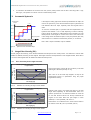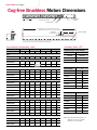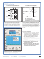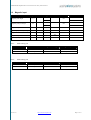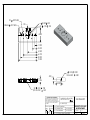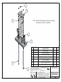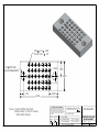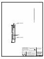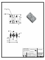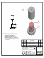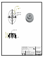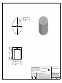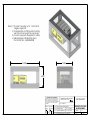
1
Sandia M.A.S.T. (Miniature Automated Shock Tester) Sponsor: Sandia National Labs Advisor: Dr. Steven Beyerlein Graduate Mentor: Kysen Palmer Team Members: Nicholai Olson Travis Nebeker Mike Brewster Fernando De La Garza Cameron Hjeltness Senior Capstone Design Work University of Idaho Final Project Report May 10, 2012 Table Of Contents 1. 2. 3. 4. 5. Executive Summary ....................................................................................................................................... 3 Background ................................................................................................................................................... 4 Problem Definition ........................................................................................................................................ 5 Project Plan ................................................................................................................................................... 6 Concepts Considered ..................................................................................................................................... 7 5.1. Design Breakup...................................................................................................................................... 7 5.2. Testing Configuration............................................................................................................................. 8 5.3. Structural Considerations....................................................................................................................... 8 5.4. Reduction of Energy Loss ....................................................................................................................... 8 5.5. Lift Actuation ......................................................................................................................................... 8 5.6. Source of Acceleration ........................................................................................................................... 9 5.7. Shock Level and Energy Dissipation ........................................................................................................ 9 6. Concept Selection ........................................................................................................................................ 11 7. Mechanical System Architecture ................................................................................................................. 13 8. Electrical Systems ........................................................................................................................................ 14 8.2 System Operation Procedure ...................................................................................................................... 14 9. Detailed Design ........................................................................................................................................... 16 9.1 Initial Prototyping ....................................................................................................................................... 16 9.2 Final Assembly ............................................................................................................................................ 18 10. Conclusions ................................................................................................................................................. 20 Recommendations ........................................................................................................................................... 21 11. Appendices .................................................................................................................................................... 22 11.1 Appendix A (Project Timeline) ................................................................................................................... 22 11.2 Appendix B (Statistical Significance of each factor) .................................................................................... 23 11.3 Appendix C (Experimental Pulse Data)....................................................................................................... 24 11.4 Appendix D (Team Budget) ....................................................................................................................... 25 11.5 Appendix E (Report on Statistical Analysis) 11.6 Appendix G (Damping Materials) 11.7 Appendix H (Linear Encoder Spec Sheet) 11.8 Appendix I (Linear Motor Spec Sheet) 11.9 Appendix J (Data Acquisition Spec Sheet) 11.10 Appendix K (Accelerometer Spec Sheet) 11.11 Appendix L (Hall Effect Sensor Board) 11.12 Appendix M (Linear Encoder Spec Sheet) 11.13 Appendix N (Thomson Rods and Linear Bearings) 11.14 Appendix M (Drawing Package) 1. Executive Summary For our senior capstone project, we have been tasked with designing a personal sized shock testing apparatus for Dr. Scott Whalen of Sandia National Labs. Shock occurs when two objects collide, causing rapid deceleration for a minute period of time. It is this impulse that Dr. Whalen wishes to measure so that he may test his proprietary electronics under these conditions. In order to accomplish this task we must first understand how to replicate these conditions with accuracy and precision, as well as how to modify them according to his user inputs. Sandia M.A.S.T. must produce shock waves within ranges of 1to 200 g’s in magnitude and 1 to 10 milliseconds in duration. Dr. Whalen will then use this apparatus that we develop and subject his electronics to these conditions, testing their reactions and developing them accordingly. Our proposal to date includes features prominent on current designs as well as other features that are unique to our design. We have determined that a dual-post shock tower with a drop table is the most appropriate for our client’s needs. To actuate this device, a linear motor is to be used with the possibility of other solutions as a backup plan. With the accuracy we plan to incorporate into our design, Dr. Whalen will have a tool that exceeds his needs and allows him to develop electronics for Sandia National Labs well beyond the scope of this project. A sub-group of our team has performed statistical analyses on the validity of our design features, with the additional motivation of being able to apply our senior design work to another class external of this project. This project has demonstrated to a 99% confidence level, that the viscoelastic damping effects will play a very significant role in comparison to impact velocity of the shock table. Through this experiment our math modeling experiments have been validated providing us with legitimate targets to shoot for in our conceptual designs and future work to be applied to this task. 2. Background Safety protocol in Dr. Whalen’s lab does not permit him to use any compressed fluids. A large majority of devices on the market use pneumatics for lift actuation as well as a system to reduce resonance. Additionally, a large majority of these are for applications where the device under test is well beyond 300 grams. Sometimes the capacity of the most basic tester is over 3300 pounds. Dr. Whalen has expressed the need for an electrically or an elastically actuated system to circumnavigate these constraints. With such a system, we feel that we will have greater controllability and reliability over other systems such as a gravity-fed drop, or a spring loaded system. Complete data sheets for each system can be referenced in the appendix of the report. Current competitor solutions include the following: AVEX SM-105,110,220 Figure 1 - Avex SM Series Shock Capacity 3- 30,000 g’s Shock Duration 0.012 [ms] to 100 [ms] Desirable Capabilities Footprint Size Able to produce three types of pulse shapes 4 [ft^2] to 15.28 [ft^2] Load capacity 50 to 200 [lbs] Table 1 Avex SM Series Specs LAB AutoShock II Shock Capacity 500- 600 g’s Shock Duration 2 [ms] to 65 [ms] Desirable Capabilities Safety interlock system Footprint Size 5.33 [ft^2] to 20 [ft^2] Load Capacity 600 [lb] Table 2 LAB AutoShock Specs Figure 2 - LAB AutoShock Lansmount 152 Shock Capacity 400 g’s Shock Duration 2.5 [ms] Desirable Capabilities Lift actuation and release mechanism Footprint Size 25 [ft^2] Load Capacity 2000 [lb] Table 3 Lansmount 152 Specs Figure 3 – Lansmount 152 LAB SD series Shock Capacity 1000 g’s to 3500 g’s Shock Duration 0.3 to 1 [ms] Desirable Capabilities Gravity actuation, small footprint. Footprint Size 0.694 [ft^2] to 2 [ft^2] Load Capacity 500 to 3300 [lb] Table 4 LAB SD Series Specs Figure 4 – LAB SD Series 3. Problem Definition A concise table of needs, specs, and targets can be viewed in Appendix A. The design will be reliable and compact, capable of measuring shocks up to 200 g’s over a range of 1-10 milliseconds, compliant with safety considerations, and will be designed for 5 or more years of performance. The device will be electrically powered and will take user input to deliver precise impulses to the device under test, while monitoring the output through LabView software. Resonance will be mitigated. 4. Project Plan Team responsibilities are delegated amongst the team. The following is a list of roles and responsibilities of each team member. Team Lead: Cameron Hjeltness Send out reminders for events, action items Create meeting agendas Run and schedule meetings Manage timeline Coordinate with POC for client meetings Coordinate with documenter for monthly status reports Budget Manager: Travis Nebeker Keep a record of expenditures Maintain a current balance of team funds Communicate with UI Department Manager Communicate with team about purchases Responsible for tracking orders Responsible for resolution of conflict with suppliers Webmaster: Fernando De La Garza Maintains up to date status of project Designs and manages team website Responsible for website deadlines and content Generates team blog Documenter: Michael Brewster Takes meeting minutes Maintains team project binder Digital file organization Check documented team deliverables Maintain team monthly reports Maintain confidentiality and legality of documentation Point of Contact: Nicholai Olson Maintain contact with; Mentor, Client, Advisor Facilitates smooth information flow between parties Relays client communication to team members and vice-versa Notifies client on team progress A current project timeline is shown in Appendix B. 5. Concepts Considered 5.1. Design Breakup Initial talks with our group concluded with eight different categories that we felt were the most important criteria for the shock tester (Table 5). Table 5 - Morphological Chart Category selection was based on necessary functions of current market offerings that we researched. Systems were broken down into mechanical, electrical, and electro-mechanical classifications. From this point we further divided the systems into quantifiable, single function categories. Safety standards as defined by Sandia National Laboratories restricted the team from exploring options involving pressurized fluids (i.e. hydraulics and pneumatics). Many shock testers on the market employ the use of high pressure fluids to lift and/or accelerate the drop tables (Figure 5). This made market research on force input only marginally helpful. Figure 5- Pneumatic Shock Testing Apparatus 5.2. Testing Configuration Our group had to decide on form of our shock tester before we could quantify options to be considered. We were provided limited spatial constraints (Appendix A) that caused our group to lean to a vertical drop device. Based on our market research, a vertical drop was unanimously chosen. The final factor that helped our group decide on a vertical structure was gravity. With a vertical design, gravity would help in acceleration of the drop table, if not provide the primary means of acceleration. 5.3. Structural Considerations Based upon research of competitors in the market, the structural design of the shock tester was limited to three categories, first being a four post design. This design is extremely stable, and strong. This allowed the reduction in diameters for the posts while keeping the strength that other designs may possess. Although a four post is stable, it would take longer to machine, and would also cost more than other design considerations. The table and posts would need to be perfectly square to keep the system from binding. Another consideration was the single post design, which was a less viable idea due to reliability and structural issues, but allowed Figure 6 - Single Post Design team members to compare ideas during the decision process (Figure 6). The platform that held the DUT would have to be balanced to prevent from binding Figure 6 - Single Post Design while being lifted and dropped for the shock. The third idea that was presented was a two post design, which most of the competitors used based on our preliminary market research (Figure 6). This design is sturdier than the single post, and will have less friction than the four post. These design considerations were incorporated in our morphological chart and house of quality, as is the case for all categories discussed below. 5.4. Reduction of Energy Loss Figure 7- Double Post Design A major concern with respect to our design was reduction of friction between the posts and the drop table. Our team researched several options to mitigate this loss. Options considered included no device, linear ball bearings, and linear bushings. The use of bushings and bearings were both valid options for a guide rod based structure, and only differed in price, percent friction reduction, and working load rating. 5.5. Lift Actuation With a drop table, there must be a lift mechanism to re-set the drop table and gain the potential energy necessary. There were a considerable number of ideas for this function, one of which being a cable and winch. Although this would be easy to control with LabView, it would be mechanically complicated. Another great idea presented was the ACME screw (Figure 8). This screw would allow the table to lift and then to drop. Although this design idea is easy to build and would be cost effective, it would need a coupling release mechanism and would only use gravity for the drop. The acceleration would be dependent upon the amount of friction that is experienced from contact with the posts, which will likely vary. The third idea presented in the morphological chart was a rotary motor and belt system. This design is not accurate, although cost effective, and would rely upon the mechanical advantage of a pulley system to provide acceleration. The last idea, a linear motor, is the most expensive but highly accurate. The linear motor will not only be able to lift the table, but accelerate the table downwards because of the ability to move in either direction with motion specified by the control system. For this option a linear encoder would likely be used. A sensor reads a magnetic strip, which allows the computer to recognize the linear motor’s displacement. The above options are dependent upon the control program that we will develop for LabView, and supply to our customer per requirements (REF Appendix A). Figure 8 – ACME Screw 5.6. Source of Acceleration Once the drop table is at its desired height, it becomes necessary to accelerate to a specified velocity to impart the desired shock. The shorter the distance, the greater the acceleration needed. To create this acceleration several options were considered. These included the use of only gravity, elastic materials, a rotary hammer, a linear motor (as stated section 5.5), a solenoid, or a motor and belt system. Advantages of gravity and springs/elastics included cost, simplicity, and availability but were lacking in repeatability. The use of a linear motor had several advantages, including the ability to accurately control and have constant feedback, as well as the elimination of several other systems, but was the most expensive option by a fair margin. For all practical purposes the option of using a solenoid system was the same as a linear motor, with the exception of being cheaper. A rotary motor and belt system would be less reliable and more mechanically complex. 5.7. Shock Level and Energy Dissipation Although pulse shapes were not a part of the project specification, Sandia M.A.S.T. wanted to pursue this as an option in order to go above and beyond. From the Senior Lab team’s results based on the comparison of drop height and viscoelastic materials, they concluded that damping materials between the table and the stopper during the shock were heavily significant to the shock peak and duration (REF Appendix C). The team used packaging foam, approximately 3mm thick per sheet, to soften the impact between the slider, where the accelerometer was mounted, and the stopper. By reading voltage charts between one and two pieces of foam, the team was able to change the pulse shape from a sharp parabolic graph to very soft sinusoidal graph (REF Appendix D). This along with changing the drop height changed the duration and amplitude of the shock. Locking mechanisms were presented to dissipate the energy, but the team believed that ringing was a problem. 6. Concept Selection The first and most fundamental design decision was that of how to orient the shock tester and how to generate the required shock. Several options were considered for this function. One idea consisted of having a horizontal sliding base that would impact against a stationary wall. Another idea was to have a stationary base hit by some sort of heavy device such as a hammer. Yet another concept consisted of a vertical tower with a sliding table that would impact a stationary base at the bottom. The structure and orientation decision matrix can be seen below (Table 6). WEIGHT FOUR POST VERTICAL TWO POST VERTICAL SINGLE POST HORIZONTAL STATIONARY BASE VERTICAL SLIDER AND HAMMER COST 20 5 3 5 3 3 MACHINABILITY 40 1 3 5 5 3 ROBUSTNESS 30 3 5 3 3 3 REPEATABILITY 50 3 5 1 3 1 DESIGN LIFE 40 3 5 5 3 3 SIZE 40 5 5 5 1 1 500 780 640 620 440 TOTAL Table 6 Decision Matrix for test apparatus structural orientation From the decision matrix, it was determined that the two post vertical drop table would be the best option. The four post design would be more difficult to manufacture and would have the potential for binding since there would be the posts have the possibility of being misaligned. A single post option was deemed to not be repeatable enough since it would be hard to keep it oriented the same way for each test. The horizontal slider option was deemed to have too large of a footprint. The stationary base and hammer option would likely have more resonance problems and in addition would likely have a shorter life because key components would be subjected to higher shocks than in the other options. After it was determined that a vertical tower would be used, it was then required to find a way to create the table motion. Ideally, an actuation method would be easy to integrate into the design, provide high controllability, and would be relatively inexpensive. Several options were considered and the results were compiled into Table 7 below. COST 40 5 3 ROTARY MOTOR & SOLENOID BELT 1 3 3 CONTROLLABILITY 30 3 3 5 1 5 20 1 3 5 1 3 40 3 5 5 1 5 30 1 3 5 3 3 460 560 640 300 620 CABLE & ACME WEIGHT WINCH SCREW EASE OF INSTALLATION STRENGTH / RELIABILTY SAFETY TOTAL LINEAR MOTOR Table 7 Table Actuation Decision Matrix The linear motor and solenoid options scored the highest due to their high controllability, ease of installation, and reliability. The cable and winch option and the rotary belt and motor option scored very low due to complexity and reliability issues. The ACME screw option had a relatively high score but the major drawback of this option was its complexity due to the many extra components that it would need. Another benefit of the linear motor and solenoid options is the fact that they require no additional components to create a downward force in order to impart shocks of the required magnitudes. These components can be easily programmed to produce different shocks. In contrast, all of the other options would likely need spring systems to create a downward force or require additional height. In an attempt to minimize size and complexity of the system, linear motors or solenoids will be used for table actuation. We hope that this decision will also help increase the system reliability and life with less components to fail and wear down with use. 7. Mechanical System Architecture The structure of the testing apparatus will be composed of a two-post vertical drop table. A detailed sketch of the conceptual design is shown below in Figure 9. Component (a) refers to the support structure of the testing apparatus to provide rigidity for the structure as a whole. Component (b) is a pair of guide rails specified from Thomson. These guide rails are to be precision machined and press fit into the top and bottom supporting structure for additional rigidity. This design will be machined with tight tolerances to reduce friction loss and prevent any binding in the bearings (e). (c) is a linear motor which imparts the force to the drop table. Component (d) is the device to be tested by the apparatus and it is mounted to the drop table (f). The device to be tested (d) will also include an accelerometer mounted to it. This accelerometer will measure the shock that the device is subjected to. An additional sensing unit, the linear encoder (i) will provide feedback of the drop table motion. Component (g) is the damping material to lessen the vibrations associated with the drop table impact, while (h) is the damping material mount. Figure 9 Conceptual drawing of the shock tester 8. Electrical Systems The control system architecture can be seen in figure 10. The system consists of a host computer, a motor controller, a motor with Hall Effect sensors, and a linear encoder. In addition, there is a data acquisition module will record the output from the accelerometer. Figure 10 System Overview During a test, the control system will first raise the table to a defined position. It will then accelerate the platform to a desired impact velocity and disable the velocity control shortly before impact. After the impact the controller will once again be enabled to position the platform back to the starting point in preparation for the next test and to avoid any secondary shocks. The systems uses a Balder Microflex e100 motor controller as the linear motor controller. The controller is an off-the-shelf controller that takes in signals from the hall effect sensor mounted on the motor as well as a differential linear encoder to control the motor position. The linear encoder is a custom mode module designed for the apparatus using an Austria microsystems AS5306A magnetic linear encoder chip. The linear encoder module has 15 micron resolution and a differential quadrature encoder output. A Data Translation DT9812A was used for the data acquisition. 8.2 System Operation Procedure Step 1) Install Labview (download evaluation version) Step 2) Install drivers Step 3) Install Open Layers library (from DAQ manufacturer) Install LV-Link ( from DAQ manufacturer) Step 4) Set up Ethernet adapter Step 5) Plug in power cord to wall and into power plug in on back of device Plug in Ethernet cord. Step 5) Open and run given Labview program Step 6) Input device address, number of cycles, desired impact velocity Hit the Go button 9. Detailed Design 9.1 Initial Prototyping During the prototyping phase of the project, we developed a series of models that helped us design the final shock tester. The first was a large steel structure built to gain an initial understanding of the process. It was constructed with ample vertical height to allow modifications as necessary. Unfortunately, assembly tolerances were very loose, creating noise in the accelerometer responses and did not provide results that could be analyzed for peak accelerations and shock duration. From this design, we did learn however that a minimal height was needed, rather than over 3 feet of vertical drop. This in turn, helped to initially validate our math model. F i g u r e 1 1 F i r s t P r o t o t y p e Our math model was further validated after moving to our next prototype, a spring-massdamper test fixture from a previous class. It was much smaller in size and built with precision rods and linear bushings. With this upgraded set of features, we obtained cleaner data with significantly less noise. We were able to determine statistical significance of the relationship between damping materials used and drop height applied. Figure 12 Last Prototype The last prototype developed had an aluminum base, precision rods, and linear bushings much like the second prototype. It was larger and more like the proposed final design. This design helped us map our machine plans in simplifying the process and to realize that we needed higher tolerances. In the end we used portions of this design on the final product. These components included high precision Thompson rods and the impact base. F i g u r e 1 3 Last Prototype 9.2 Final Assembly The final design is shown in Figure 14. There is a large degree of similarity to Figure 9 displaying our conceptual design. (A) shows the DUT fixture which mounts to hole pattern as specified by Sandia Labs. (B) represents the Thomson rods, allowing (C), the drop table, to slide smoothly with a high degree of mechanical tolerance. (D) is the damping material mounted to component (E) which is a component derived from our third prototype. (F) is our wooden base, constructed of maple hardwood. (G) shows our linear encoder which relays information of the table’s position to within 15 micron to component (J), the linear motor. (J) is regulated by (K), the linear motor controller. Our specifications for the design were provided by the client and served to guide our design from beginning to end. Listed with a description, they are in the following table. GENERAL NEED Physical constraints SPECIFIC REQUIREMENT Small Size TARGET VALUES Standardized mounting interface Maximum base dimension of 30” square and height of 72”. 1.5” center 3/8” -16; course thread Standardized DUT to contain proprietary electronics Cylinder of diameter 5 cm, length 8 cm, mass of 0.3 kg. Instrumentation Performance Requirements Electrical Energy Input Measure shock in X direction Measure shock in Y direction Measure shock in Z direction Voltage response will be measured upon impact. Shock and voltage response monitored DUT must not experience ringing. Accurate Repeatable Safety/Robustness Pinch Points Protected Electrical Connections Protected Long life 120 V AC Electric Motors, Solenoids, etc. 100g’s to 200g’s 100g’s to 200g’s 100g’s to 200g’s 0 to 10 Volts LabView Software; High bit rate data acquisition device Single pulse half sine wave. Calibrated to Input Correct Levels of Shock Perform numerous similar tests with consistent results Physical Shielding No exposed wiring or electrical components Perform several hundred tests per month for a desired life of five years. 10. Conclusions The goal of this project was to provide Sandia Labs with a reliable mechanical shock tester for their proprietary electronics within the operating conditions of 100 to 200 g’s and limiting the applied shock to within 10 milliseconds. While not the most complex task, this design posed many challenges of its own that proved to be a good resource for future knowledge. Machining some of the components such as the arm that mounts to the linear motor to transmit the force through the dual steel rods were tricky, requiring a detailed machine plan and the knowhow to deriving the correct geometry within tolerances. The electronic systems proved to be more complex than originally planned, with many various parts. Designing and fabricating the linear encoder boards involved large amounts of time planning each component. Overall, the project’s goals were certainly met. The accelerometer mounted to the surface of the device under test registered shocks within 175 g’s which is within 12.5% of the intended upper range of operation. The size was limited to be as small as reliably possible. This was not an explicit design constraint given to Sandia MAST, however from talks with the client and other specs given, it was evident that size was an issue. Physically the shock tester was required to stay within 30” wide by 30” long by 72” tall. The end design captured much less territory with dimensions of 14” x 7.75” by 22”. In achieving the end-goal of this project, Sandia MAST has capably demonstrated that a mini shock tester is viable and produced a working model from which further designs can be fabricated. Recommendations Short-Term Recommendations for Sandia National Labs are as follows: 1. Replace the Hall-effect sensor board as seen in Appendix L. 2. Fabricate more damping samples per manufacturer’s instructions in Appendix G. 2.1. 3. Use damping caster and bases. Re-fabricate damping caster and bases per drawing package. The old ones were discarded accidentally. 4. 5. 6. Never operate without damping sample. Install photo-gate interrupter to avoid crashes into underside of aluminum base on the up-stroke. Mill slot into base to include clearance for Hall-effect sensor. Long-Term Reccomendation for Sandia National Labs are as follows: 1. 2. 3. 4. 5. The shock tester must be mounted to a solid workbench table to reduce noise. Lubricate Thomson rods with graphite powder as necessary. Provide adequate safety measures to ensure no injuries are incurred during operation. Do not operate without plexi-glass panels installed. If disassembled, reassemble with blue Loctite on all metal-to-metal fasteners. 11. Appendices 11.1 Appendix A (Project Timeline) 11.2 Appendix B (Statistical Significance of each factor) 11.3 Appendix C (Experimental Pulse Data) Figure 11: Drop Height: 8.5 cm Damper Thickness: 3 mm Peak Acceleration: 210 g Pulse Duration: 3.7 ms Figure 83: Drop Height: 8.5 cm Damper Thickness: 6 mm Peak Acceleration: 51 g Pulse Duration: 11 ms Figure 72: Drop Height: 15.5 cm Damper Thickness: 3mm Peak Acceleration: 272 g Pulse Duration: 3.7 ms Figure 14: Drop Height: 15.5 cm Damper Thickness: 6 mm Peak Acceleration: 77 g Pulse Duration: 9.5 ms 11.4 Appendix D (Team Budget) 11.5 Appendix E (Report on Statistical Analysis) Shock Pulses and the Effects Contributed by Viscoelastic Damping Materials Submitted to: Dr. Denise Bauer 709 Deakin Avenue Moscow, ID 83843 Submitted by: Cameron Hjeltness Department of Mechanical Engineering University of Idaho Michael Brewster Department of Mechanical Engineering University of Idaho December 13, 2011 Shock pulses and the effects contributed by viscoelastic damping materials (December 2011) C. B. Hjeltness, M. Brewster School of Mechanical Engineering, University of Idaho, Engineering Campus, Idaho, U.S.A. Abstract: Senior design team, Sandia M.A.S.T. (Miniature Accelerations Shock Tester) has been tasked with designing a shock testing apparatus for Dr. Scott Whalen of Sandia National Labs. Shock occurs when two objects collide, causing rapid deceleration for minute periods of time. It is this impulse that Dr. Whalen wishes to measure so that he may test his proprietary electronics under specific conditions of 1 to 10 milliseconds, and up to 200 g’s. In order to accomplish this task, an understanding of how to replicate these conditions with accuracy and precision, as well as how to modify them according to his user inputs is to be gained. Current published information lacks uniformity and reliability, leaving the team with nothing better than educated guesses. This paper publishes findings from an experiment testing how the thickness and properties of certain materials affect shock pulse duration and magnitude, how height affects shock pulse duration and magnitude, and which factor is more significant. Statistical analyses of Factorial Regressions were performed determining that of the two selected for observation, the thickness of the viscoelastic material used is the most important factor with a statistical confidence of 99%. Key Words: I. shock, viscoelastic, drop height, factor, factorial regression, accelerometer INTRODUCTION T HIS document describes the work done by members of Sandia M.A.S.T. for their senior capstone project. Shock testers are used in industry to subject components or entire structures to shock over a regulated period of time. They range in form, function, cost, methods of actuation, and applicable standards to which they apply. There are multiple methods of accomplishing shock tests in the industry including pyrotechnics, hammer, and classical shock testing [1]. For the scope of this project, a classical shock testing apparatus is to be built and implemented according to Dr. Whalen of Sandia National Labs. This implies a vertical drop table with a means of actuation and a vertical post construction. The information gained from this experiment will supplement the current senior design team with informed data, allowing the delivery of a precision instrument to Dr. Whalen. Being that this is the first time that this project has been instituted, this information will be forwarded onward to next year’s design team who will repeat or carry onward with this design task, building from what we accomplish this year. The ability to have the information that we discover will save next year’s team countless hours and reserve funds for proper allocation, new developments on the project. A basic understanding of physical phenomena is crucial to designing the shock tower to the specifications provided. Dr. Whalen will have other applications that he does not yet know of or that he does not currently realize. If the solution delivered to him exceeds expectations, he will no doubt find it significantly more useful than originally anticipated, making the return on investments into these efforts worthwhile. It is the desire of my team to deliver a product to Sandia National Labs that exceeds these expectations allowing Dr. Whalen the continued use of our product. Additionally, the outcome of this design will undoubtedly influence the net worth of the degrees of each team member, Manuscript received December 13, 2011. This work was supported in part by Sandia National Labs and the University of Idaho. C. B. Hjeltness is with the University of Idaho mechanical engineering department, Moscow, Idaho 83843 USA. Phone: 208-819-2257. Email: [email protected]. M. Brewster is with the University of Idaho mechanical engineering department, Moscow, Idaho 83843 USA. Phone: 425-765-6406. Email: [email protected]. playing a direct role in our ability to be hired in the industry or to move on to graduate school. The aim of a senior design project is to be a showcase of the talents of each team member as an engineer. Producing a product compliant to published industry standards that exceeds the expectations of my sponsor would have a great impact on my overall livelihood as well as that of the rest of my team mates and teams to come in the future. II. METHODS 1. Data Analysis and Test Constraints To analyze the data, a factorial regression using Microsoft Excel is to be performed. AFactorial analysis is a common method of analyzing the importance and interaction of different factors of experimental data. This allows testing of a hypothesis when there are two or more independent variables. Drop height and the thickness of the viscoelastic material were the two independent variables in this experiment, compared to the dependent variables of the shock amplitude and the pulse duration. By compiling and analyzing data using a factorial ANOVA table, comparisons the two were made allowing the discovery of which is more important to the dependent variables. This analysis will tell the team which factor, if any, is significant to both the magnitude of the pulse and the duration for which the pulse lasts. I will also be able to determine which material to use for a damping platform on the senior design project that will provide the optimum results with high accuracy and minimal resonance. Should the analysis prove that no factor is statistically significant, this will show that there is another physical phenomenon that needs explanation. The more likely outcome is that one factor will emerge as the most significant. This will drive the design choices, and resources of my design team, Sandia M.A.S.T. An accelerometer purchased from PCB Piezotronics is the Figure 1 - Prototype used for testing sensing element utilized for this project. The sensitivity is advertised online 10 mV/g with an accuracy of +15 percent. Our specific unit has sensitivity calibrations of 10.36 mv/g, 10.31 mv/g, and 10.29 mv/g for the x, y, and z axes respectively. In order to derive useful data to the rest of the University and to be able to apply it in industry, tests adhere to current standards for performing shock tests. Available at the team’s disposal are military specifications to guide the experiment. MIL-S-901D(NAVY) describes shock test procedures [2], and MIL-STD-810F describes test conditions such as temperature, humidity, and most importantly the accuracy to which shocks from acceleration are to be measured [3]. 2. Test Apparatus Figure 1 shows the conceptual design for the purposes of the designed experiment. Component (a) refers to the top and bottom portion of the apparatus. Constructed of inexpensive aluminum, its function is to provide a solid base that is level and will restrict the level of permissible resonance. Component (b) shows precision guide rails. These will be costly with respect to the structural components because they will be machined to tight tolerances to avoid interference with components (d). Components (c) and (h) display the sensors associated with the system. (c) shows the accelerometer, the most costly component with which I will collect the primary data samples. (h) is a conceptual component, a magnetic linear encoder which provides exact calibrated position and velocity. Included with (h) is a sensing magnet also shown in green. I will use this data alongside a mathematic model to compare theoretical and experimental values. Component (d) is the energy reduction system, bushings, which will allow smooth and repeatable drops. Resonance is unacceptable and will be limited. For these purposes I have chosen brass as a suitable material from which to construct component (e), or the drop table. (f) denotes the polymer sample, which is atop component (g), a mounting platform. III. EXPERIMENTAL DESIGN 2. Statistical Models 1. Capstone math models A primary objective of this project is to verify the mathematical models for the capstone project. This model demonstrates the necessary drop height for a gravity-actuated system, as well as what damping coefficient would be best for our design targets. Equation (1) is the model used to describe the acceleration of the impact with respect to time. For the statistical analysis, two factors were analyzed. The first factor was drop height. This factor is directly proportional to the amount of acceleration an object experiences during free fall motion. It is important to note that this acceleration is different from the pulse experienced during impact; however it is still vital for this experiment as it shows what input force is necessary to achieve the impact. The second variable examined was the thickness of the damping material used. Both independent variables, they were measured with respect to the dependent variables, pulse magnitude and pulse duration. (1) A list of the relevant variables for this equation is listed in Table 1 below. Symbol Units Description m kg Mass of Drop Table y_1 m Displacement y_2 m/s Velocity y_3 m/s^2 Acceleration of Table g m/s^2 Acceleration of Gravity k_b N/m Spring Stiffness c_b kg-s/m Damping Coefficient Table 1 - List of relevant variables Figure 2 shows the output of this model, y3, when run with values for the independent variables of (1). Appendix A contains the full code used to generate this plot. Foam was the damping material chosen for this experiment. Specifically ESD (Electro-Static Dissipating) foam, it was readily accessible and abundant in quantity. Its damping materials were deemed sufficient enough for prototyping and testing procedures. Young’s modulus for such foams is determined to be within a range of 0.08 to 0.93 MPa [4]. This means that it is a fairly soft material in comparison with Steel of 210 Gpa [5], and justified the decision to use it as a material with which to modify the pulse. The values of this independent variable ranged from 3 mm thick for one pad to 6 mm thick for two pads. This variable was determined at a confidence of 95% Drop height was chosen experimentally. Tests were performed to conform to the design targets. Thus, at a maximum of two pads of foam, a maximum drop height was determined to be 15.5 cm since the resulting maximum g’s experienced by the accelerometer was 250 in amplitude. With 15.5 cm as the maximum value for this variable, the minimum value was set arbitrarily as 8.5 cm. This resulted in a minimum of around 50 g’s, suitable for the given range of experimental accelerations. This variable was determined at a confidence of 95%. Table 3 below summarizes the independent variables: Table 2 - Dependent variables and the applied ranges Figure 2 - Mathematical model for shock response IV. Experimental Procedure 1. Equipment used Below is a list of equipment utilized during the experiment: Digital Multi-meter Oscilloscope Accelerometer Foam-pads (1” by 1”) Mounting platform for foam Drop test device Measuring tape Mounting wax 2. Setup The experimental setup was fairly basic and had only a few steps. First, the drop test device was secured such that it would not move to maintain test consistency. Next, the measuring tape was secured next to the drop tester and secured. The accelerometer was affixed with the mounting wax and connected to the oscilloscope. The settings on the oscilloscope were set at 1.00 volts per vertical division, and 2 milliseconds per time division. 3. Procedure The table of the drop tester was raised to a height of 8.5 cm from the initial position atop one pad of foam. With the oscilloscope ready to capture data, the table was released and a pulse was recorded. This was repeated 10 times, replacing the foam for every iteration. This process was imitated at 15.5 cm with one pad of foam, 8.5 cm and two pads of foam, and finally at 15.5 cm and two pads. 40 unique data points were collected. Each data point collected further data on the two dependent variables, and thus 80 data points in all were effectively gathered. APPENDIX A MATLAB CODE USED TO MODEL THE RESPONSE TO ACCELERATION PULSES % Drop Table Simulation clear all close all % %% Assumptions: % - Structure of Drop table and supporting mechanisms is assumed to be rigid. % > No energy is lost structures, perfectly elastic collision. % > Deformation in stopping object does not exceed material yield poing % > No deformation occurs in colliding body. % %% Parameters % m=2.0 % Mass of drop table [kg] d=0.08 % Diamter of base [m] L=0.04 % Length of base [m] A=pi/4*d^2 % Cross Sectional Area [m^2] E=0.1e9 % Young's Modulus of Rubber [Pa] % g=9.81 % Acceleration of Gravity [m/s^2] k_b=A*E/L % Spring stiffness [N/m] c_b=100 % Damping Coefficient [kg-s/m] % param.m=m param.k_b=k_b param.c_b=c_b param.g=g % %% Time Array % N=10000 tend=0.1 % End simulation at t=0.01 seconds t=linspace(0,tend,N) dt=t(2)-t(1) % xo(1)=0 % Initial Position [m] xo(2)=-0.5 % Initial Velocity [m/s] % %% ODE 45 Simulation % [t,x]=ode45(@(t,xo) impact(t,xo,param),t,xo); % Call ODE45 % %% Outputs % y1=x(:,1) % Displacement [m] y2=x(:,2) % Velocity [m/s] for i=1:length(y1) gravity before impact if y1(i)<0 y3(i)=-g-y1(i)*k_b/m-y2(i)*c_b/m; else y3(i)=-g; end end % % Acceleration is equal to %% Plots % subplot(3,1,1) plot(t,y1) title('Displacement of Drop Table') axis([0 0.01 min(y1) max(y1)]) legend('x1') ylabel('Displacement [m]') % subplot(3,1,2) plot(t,y2) title('Velocity of Drop Table') axis([0 0.01 min(y2) max(y2)]) ylabel('Velocity [m/s]') % subplot(3,1,3) plot(t,y3) title('Accleration of Drop Table') ylabel('Acceleration [m/s^2]') xlabel('Time (s)') axis([0 0.01 min(y3) max(y3)]) maxacc=max(y3) table % Maximum Acceleration of drop REFERENCES [1] [2] “MIL-S-901 Rev. D,” http://www.everyspec.com/MIL SPECS/MIL+SPECS+(MIL-S)/MIL-S-901D_14581/ [3] H. Egbert, “MIL-STD-810F,” 2000, http://www.dtc.army.mil/navigator/ [4] http://www.biomedcentral.com/1471-2474/9/137 [5] Gere, James. Mechanics of Materials. 8. 2009. 26. Print. [6] 11.6 Appendix G (Damping Materials) PMC®-746 Polyurethane Rubber Compound www.smooth-on.com PRODUCT OVERVIEW PMC®-746 was developed to make molds for casting gypsum plasters. Like PMC®-744, this product is well suited for use as a rubber case mold – especially large case molds where extra rigidity is required. Shore hardness is 60A. Because of its durability and moisture resistant properties PMC®-746 is also used by zoos and museums for a variety of mold-making, display and exhibit applications. It features a convenient mix ratio (2:1 by weight or volume), and contains no mercury. Other applications include making plaster block molds, reproducing ornamental plaster (architectural restoration), pre-cast concrete molds, casting waxes, Smooth-On rigid polyurethanes and epoxies and also for making a variety of special effects for movies and theatre. PROCESSING RECOMMENDATIONS START BY PREPARING YOUR MODEL... Preparation - Materials should be stored and used in a warm environment (73°F/23°C). They also have a limited shelf life and should be used as soon as possible. Wear safety glasses, long sleeves and rubber gloves to minimize contamination risk. Some Materials Must Be Sealed - To prevent adhesion between the rubber and model surface, models made of porous materials (gypsum plasters, concrete, wood, stone, etc.) must be sealed prior to applying a release agent. SuperSeal® or One Step® (available from Smooth-On) are fast drying sealers suitable for sealing porous surfaces without interfering with surface detail. A high quality spray shellac is suitable for sealing modeling clays that contain sulfur or moisture (water based). Thermoplastics (polystyrene) must also be sealed with shellac or PVA. TECHNICAL OVERVIEW Mix Ratio: 2A : 1B by weight or volume Mixed Viscosity (cps): 1,200 (ASTM D-2393) Specific Gravity (g/cc): 1.03 (ASTM D-1475) Specific Volume (cu. in. /lb.): 26.9 Pot Life: 15 minutes (73°F/23°C) (ASTM D-2471) In all cases, the sealing agent should be applied and allowed to completely dry prior to applying a release agent. Non-Porous Surfaces - Metal, glass, hard plastics, sulfur free clays, etc. require only a release agent. Applying A Release Agent - A release agent is necessary to facilitate demolding when casting into or over most surfaces. Use a release agent made specifically for mold making (Universal® Mold Release available from Smooth-On). A liberal coat of release agent should be applied onto all surfaces that will contact the rubber. IMPORTANT: To ensure thorough coverage, lightly brush the release agent with a soft brush over all surfaces of the model. Follow with a light mist coating and let the release agent dry for 30 minutes. Cure time: 16 hours (73°F/23°C) Color: Amber (color may vary from batch to batch) Because no two applications are quite the same, a small test application to determine suitability for your project is recommended if performance of this material is in question. Shore A Hardness: 60 (ASTM D-2240) Tensile Strength (psi): 700 (ASTM D-412*) MEASURING & MIXING... 100% Modulus (psi): 220 (ASTM D-412*) Elongation @ Break: 650% (ASTM D-412*) Die C Tear Strength (pli): 100 (ASTM D-624*) Liquid urethanes are moisture sensitive and will absorb atmospheric moisture. Mixing tools and containers should be clean and made of metal, glass or plastic. Materials should be stored and used in a warm environment (73°F/23°C). Shrinkage: < .001 in./in. (ASTM D-2566*) * Value measured after 7 days at 73°F/23° IMPORTANT: Shelf life of product is drastically reduced after opening. Immediately replacing the lids on both containers after dispensing product will prolong the shelf life of the unused product. XTEND-IT® Dry Gas Blanket (available from Smooth-On) will significantly prolong the shelf life of unused liquid urethane products. IMPORTANT: Shelf life of product is reduced after opening. Remaining product should be used as soon as possible. Immediately replacing the lids on both containers after dispensing product will help prolong the shelf life of the unused product. XTEND-IT® Dry Gas Blanket (available from Smooth-On) will significantly prolong the shelf life of unused liquid urethane products. IMPORTANT: Pre Mix the Part B before using. After dispensing two Parts A and one Part B into mixing container, mix thoroughly for at least 3 minutes making sure that you scrape the sides and bottom of the mixing container several times. Safety First! The Material Safety Data Sheet (MSDS) for this or any Smooth-On product should be read prior to use and is available upon request from SmoothOn. All Smooth-On products are safe to use if directions are read and followed carefully. Be careful Part A is a TDI prepolymer. Vapors, which can be significant if material is heated or sprayed, cause lung damage and sensitization. Use only with adequate ventilation. Contact with skin and eyes may cause severe irritation. Flush eyes with water for 15 minutes and seek immediate medical attention. Remove from skin with waterless hand cleaner followed by soap and water Prepolymers contain trace amounts of TDI which, if ingested, must be considered a potential carcinogen. Refer to MSDS . If Mixing Large Quantities (16 lbs./7 kgs. or more) at one time, use a mechanical mixer (i.e. Squirrel Mixer or equal) for 3 minutes followed by careful hand mixing for one minute as directed above. Then, pour entire quantity into a new, clean mixing container and do it all over again. Although this product is formulated to minimize air bubbles in your the cured rubber, vacuum degassing will further reduce entrapped air. A pressure casting technique using a pressure chamber can yield totally bubble free molds. Contact Smooth-On or your distributor for further information about vacuum degassing or pressure casting. POURING, CURING & PERFORMANCE... Pouring - For best results, pour your mixture in a single spot at the lowest point of the containment field. Let the rubber seek its level up and over the model. A uniform flow will help minimize entrapped air. The liquid rubber should level off at least 1/2” (1.3 cm) over the highest point of the model surface Curing - Allow rubber to cure overnight (at least 16 hours) at room temperature Part B is irritating to the eyes and skin. If contaminated, flush eyes with water for 15 minutes and seek immediate medical attention. Remove from skin with soap and water. When mixing with Part A follow precautions for handling isocyanates. (73°F/23°C) before demolding. Cure time can be reduced with mild heat or by adding Smooth-On “Kick-It®” Cure Accelerator. Do not cure rubber where temperature is less than 65°F/18°C. Important: The information contained in this bulletin is considered accurate. However, no warranty is expressed or implied regarding the accuracy of the data, the results to be obtained from the use thereof, or that any such use will not infringe upon a patent. User shall determine the suitability of the product for the intended application and assume all risk and liability whatsoever in connection therewith. Using The Mold - If using as a mold material, a release agent should be Post Curing - After rubber has cured at room temperature, heating the rubber to 150°F (65°C) for 4 to 8 hours will increase physical properties and performance. applied to the mold before each casting. The type of release agent to use depends on the material being cast. The proper release agent for wax, liquid rubber or thermosetting materials (i.e. Smooth-On liquid plastics) is a spray release made specifically for mold making (available from Smooth-On or your distributor). Prior to casting gypsum plaster materials, sponge the mold with a soap solution for better plaster flow and easy release. In & Out® II Water Based Release Concentrate (available from Smooth-On) is recommended for releasing abrasive materials like concrete. Performance & Storage - Fully cured rubber is tough, durable and will perform if properly used and stored. The physical life of the rubber depends on how you use it. Call Us Anytime With Questions About Your Application. Toll-free: (800) 762-0744 Fax: (610) 252-6200 The new www.smooth-on.com is loaded with information about mold making, casting and more. 052511 - JR PMC®-780 Dry & PMC®-780 Wet Industrial Liquid Rubber Compounds www.smooth-on.com PRODUCT OVERVIEW PMC-780 is a premium performance urethane rubber that offers exceptional strength, durability and abrasion resistance. PMC-780 DOES NOT CONTAIN MOCA – a known cancer causing agent and hazard. Mixed two parts A to one part B by weight, PMC-780 pours easily and cures at room temperature with negligible shrinkage to a solid Shore 80A rubber. Pick The One Best Suited For Your Application: Original PMC-780 Dry does not exude oil. New PMC-780 Wet contains a builtin release agent to aid in demolding concrete. (Note: “wet” rubber has a higher net shrinkage value over time vs. “dry “ rubber.) Both are used around the world for casting abrasive materials such as concrete (pre-cast concrete, making concrete stamping pads, etc.) and gypsum plasters with high exotherms. PMC-780 Dry is also commonly used to make rubber mechanical parts of varying configurations (gaskets, wheels, and pullies) as well as ball mill liners and vibration/shock pads. PROCESSING RECOMMENDATIONS START BY PREPARING YOUR MODEL... Preparation - These products have a limited shelf life and should be used as soon as possible. Materials should be stored and used at room temperature (73°F/23°C). Humidity should be low. Wear safety glasses, long sleeves and rubber gloves to minimize contamination risk. Good ventilation (room size) is necessary. Some Materials Must Be Sealed - To prevent adhesion between the rubber and model surface, models made of porous materials (gypsum plasters, concrete, wood, stone, etc.) must be sealed prior to applying a release agent. SuperSeal® or One Step® (available from Smooth-On) is a fast drying sealer suitable for sealing porous surfaces without interfering with surface detail. You can also use Sonite® Wax. A high quality Shellac is suitable for sealing modeling clays that contain sulfur or moisture (water based). TECHNICAL OVERVIEW Mix Ratio: 2A : 1B by weight or volume Mixed Viscosity (cps): 2,000 (ASTM D-2393) Specific Gravity (g/cc): 1.02 (ASTM D-1475) Specific Volume (cu. in. /lb.): 27.2 Pot Life: 25 minutes (73°F/23°C) (ASTM D-2471) In all cases, the sealing agent should be applied and allowed to completely dry prior to applying a release agent. Non-Porous Surfaces - Metal, glass, hard plastics, sulfur free clays, etc. require only a release agent. Applying A Release Agent - A release agent is necessary to facilitate demolding when casting into or over most surfaces. Use a release agent made specifically for mold making (Universal® Mold Release available from Smooth-On). A liberal coat of release agent should be applied onto all surfaces that will contact the rubber. IMPORTANT: To ensure thorough coverage, lightly brush the release agent with a soft brush over all surfaces of the model. Follow with a light mist coating and let the release agent dry for 30 minutes. Cure time: 48 hrs (73°F/23°C) Color: Light Amber Because no two applications are quite the same, a small test application to determine suitability for your project is recommended if performance of this material is in question. Shore A Hardness: 80 (ASTM D-2240) Tensile Strength (psi): 900 (ASTM D-412) 100% Modulus (psi): 400 (ASTM D-412) Elongation @ Break: 700% (ASTM D-412) Liquid urethanes are moisture sensitive and will absorb atmospheric moisture. Mixing tools and containers should be clean and made of metal or plastic. Die C Tear Strength (pli): 200 (ASTM D-624) IMPORTANT: Shelf life of product is drastically reduced after opening. Shrinkage: < .001 in./in. (ASTM D-2566) * All values measured after 7 days at 73°F/23°C MEASURING & MIXING... Immediately replacing the lids on containers after dispensing product will prolong the shelf life of the unused product. XTEND-IT® Dry Gas Blanket (available from Smooth-On) will significantly prolong the shelf life of unused liquid urethane products. IMPORTANT: Shelf life of product is reduced after opening. Remaining product should be used as soon as possible. Immediately replacing the lids on both containers after dispensing product will help prolong the shelf life of the unused product. XTEND-IT® Dry Gas Blanket (available from Smooth-On) will significantly prolong the shelf life of unused liquid urethane products. IMPORTANT: Pre Mix the Part B before using. After dispensing the required amounts of Parts A and B into mixing container, mix thoroughly for at least 3 minutes making sure that you scrape the sides and bottom of the mixing container several times. Safety First! The Material Safety Data Sheet for this or any Smooth-On product should be read before using and is available upon request. All Smooth-On products are safe to use with proper handling and precautions. Read and follow directions carefully. Be careful Part A is a TDI prepolymer. Vapors, which can be significant if prepolymer is heated or sprayed, may cause lung damage and sensitization. Use only with adequate ventilation. Contact with skin and eyes may cause severe irritation. Flush eyes with water for 15 minutes and seek immediate medical attention. Remove from skin with soap and water. Prepolymers contain trace amounts of TDI which, if ingested, must be considered a potential carcinogen. Refer to the MSDS for this product. Avoid skin contact by wearing long sleeve garments and latex gloves. If skin contact is made, remove immediately with soap and water. If eye contact is made, flush eyes with water for 15 minutes and seek immediate medical attention. Important: The information contained in this bulletin is considered accurate. However, no warranty is expressed or implied regarding the accuracy of the data, the results to be obtained from the use thereof, or that any such use will not infringe a patent. User shall determine the suitability of the product for its intended applications and assumes all risk and liability whatsoever in connection therewith. If Mixing Large Quantities (24 lbs./11 kgs. or more) at one time, we suggest using a mechanical mixer (i.e. Squirrel Mixer or equal) for 3 minutes followed by careful hand mixing for one minute as directed above. Then, pour entire quantity into a new, clean mixing container and do it all over again. Although this product is formulated to minimize air bubbles in the cured rubber, vacuum degassing will further reduce entrapped air. A pressure casting technique using a pressure chamber can yield totally bubble free castings. Contact SmoothOn or your distributor for further information about vacuum degassing or pressure casting. POURING, CURING & PERFORMANCE... Pouring - For best results, pour your mixture in a single spot at the lowest point of the containment field. Let the rubber seek its level up and over the model. A uniform flow will help minimize entrapped air. The liquid rubber should level off at least 1/2” (1.3 cm) over the highest point of the model surface. Curing - Allow the mold to cure (at least 48 hours) at room temperature (73°F/23°C) before demolding. Do not cure rubber in temperatures less than 65°F/18°C. Cure time can be reduced with mild heat or by adding Smooth-On “Kick-It®” Cure Accelerator. Post Curing - After rubber has cured at room temperature, heating the rubber to 150°F (65°C) for 4 to 8 hours will increase physical properties and performance. Using The Mold - If using as a mold material, a release agent should be applied to the mold before each casting. The type of release agent to use depends on the material being cast. The proper release agent for wax, liquid rubber or thermosetting materials (i.e. Smooth-On liquid plastics) is a spray release made specifically for mold making (available from Smooth-On or your distributor). Prior to casting gypsum plaster materials, sponge the mold with a soap solution for better plaster flow and easy release. In & Out® II Water Based Release Concentrate (available from Smooth-On) is recommended for releasing abrasive materials like concrete. Performance & Storage - Fully cured rubber is tough, durable and will perform if properly used and stored. The physical life of the rubber depends on how you use it. Contact Smooth-On directly with questions about this material relative to your application. Call Us Anytime With Questions About Your Application. Toll-free: (800) 762-0744 Fax: (610) 252-6200 The new www.smooth-on.com is loaded with information about mold making, casting and more. 071910 - JR PMC®-770 Industrial Liquid Rubber Compound www.smooth-on.com PRODUCT OVERVIEW PMC®-770 is a Shore 70A addition to our line of industrial liquid rubber products (such as PMC®-780 and PMC®-790) used for a variety industrial and casting applications. Mixed two parts A to one part B by weight, PMC®-770 pours easily and cures at room temperature to a solid Shore 70A rubber that has exceptional performance characteristics and dimensional stability. It is suitable for production casting of abrasive materials such as concrete (pre-cast concrete, making concrete stamping pads, etc.) and gypsum plasters with high exotherms. It is also suitable for rubber mechanical parts of varying configurations (gaskets, wheels, pullies) as well as ball mill liners and vibration/shock pads. PROCESSING RECOMMENDATIONS START BY PREPARING YOUR MODEL... Preparation - These products have a limited shelf life and should be used as soon as possible. Materials should be stored and used at room temperature (73°F/23°C). Humidity should be low. Wear safety glasses, long sleeves and rubber gloves to minimize contamination risk. Good ventilation (room size) is necessary. Some Materials Must Be Sealed - To prevent adhesion between the rubber and model surface, models made of porous materials (gypsum plasters, concrete, wood, stone, etc.) must be sealed prior to applying a release agent. SuperSeal® or One Step® (available from Smooth-On) is a fast drying sealer suitable for sealing porous surfaces without interfering with surface detail. You can also use Sonite® Wax. A high quality Shellac is suitable for sealing modeling clays that contain sulfur or moisture (water based). TECHNICAL OVERVIEW Non-Porous Surfaces - Metal, glass, hard plastics, sulfur free clays, Mix Ratio: 2A : 1B by weight etc. require only a release agent. Mixed Viscosity (cps): 3,000 (ASTM D-2393) Specific Gravity (g/cc): 1.04 (ASTM D-1475) Specific Volume (cu. in. /lb.): 26.5 Pot Life: 30 minutes (73°F/23°C) In all cases, the sealing agent should be applied and allowed to completely dry prior to applying a release agent. (ASTM D-2471) Applying A Release Agent - A release agent is necessary to facilitate demolding when casting into or over most surfaces. Use a release agent made specifically for mold making (Universal® Mold Release available from Smooth-On). A liberal coat of release agent should be applied onto all surfaces that will contact the rubber. IMPORTANT: To ensure thorough coverage, lightly brush the release agent with a soft brush over all surfaces of the model. Follow with a light mist coating and let the release agent dry for 30 minutes. Cure time: 16 hrs (73°F/23°C) Color: Light Amber Because no two applications are quite the same, a small test application to determine suitability for your project is recommended if performance of this material is in question. Shore A Hardness: 70 (ASTM D-2240) Tensile Strength (psi): 750 (ASTM D-412) 100% Modulus (psi): 250 (ASTM D-412) Elongation @ Break: 750% (ASTM D-412) Liquid urethanes are moisture sensitive and will absorb atmospheric moisture. Mixing tools and containers should be clean and made of metal or plastic. Die C Tear Strength (pli): 200 (ASTM D-624) IMPORTANT: Shelf life of product is drastically reduced after opening. Shrinkage: < .001 in./in. (ASTM D-2566) * All values measured after 7 days at 73°F/23°C MEASURING & MIXING... Immediately replacing the lids on containers after dispensing product will prolong the shelf life of the unused product. XTEND-IT® Dry Gas Blanket (available from Smooth-On) will significantly prolong the shelf life of unused liquid urethane products. IMPORTANT: Shelf life of product is reduced after opening. Remaining product should be used as soon as possible. Immediately replacing the lids on both containers after dispensing product will help prolong the shelf life of the unused product. XTEND-IT® Dry Gas Blanket (available from Smooth-On) will significantly prolong the shelf life of unused liquid urethane products. IMPORTANT: Pre Mix the Part B before using. After dispensing the required amounts of Parts A and B into mixing container, mix thoroughly for at least 3 minutes making sure that you scrape the sides and bottom of the mixing container several times. Safety First! The Material Safety Data Sheet for this or any Smooth-On product should be read before using and is available upon request. All Smooth-On products are safe to use with proper handling and precautions. Read and follow directions carefully. Be careful Part A is a TDI prepolymer. Vapors, which can be significant if prepolymer is heated or sprayed, may cause lung damage and sensitization. Use only with adequate ventilation. Contact with skin and eyes may cause severe irritation. Flush eyes with water for 15 minutes and seek immediate medical attention. Remove from skin with soap and water. Prepolymers contain trace amounts of TDI which, if ingested, must be considered a potential carcinogen. Refer to the MSDS for this product. Avoid skin contact by wearing long sleeve garments and latex gloves. If skin contact is made, remove immediately with soap and water. If eye contact is made, flush eyes with water for 15 minutes and seek immediate medical attention. Important: The information contained in this bulletin is considered accurate. However, no warranty is expressed or implied regarding the accuracy of the data, the results to be obtained from the use thereof, or that any such use will not infringe a patent. User shall determine the suitability of the product for its intended applications and assumes all risk and liability whatsoever in connection therewith. If Mixing Large Quantities (24 lbs./11 kgs. or more) at one time, we suggest using a mechanical mixer (i.e. Squirrel Mixer or equal) for 3 minutes followed by careful hand mixing for one minute as directed above. Then, pour entire quantity into a new, clean mixing container and do it all over again. Although this product is formulated to minimize air bubbles in the cured rubber, vacuum degassing will further reduce entrapped air. A pressure casting technique using a pressure chamber can yield totally bubble free castings. Contact SmoothOn or your distributor for further information about vacuum degassing or pressure casting. POURING, CURING & PERFORMANCE... Pouring - For best results, pour your mixture in a single spot at the lowest point of the containment field. Let the rubber seek its level up and over the model. A uniform flow will help minimize entrapped air. The liquid rubber should level off at least 1/2” (1.3 cm) over the highest point of the model surface. Curing - Allow the mold to cure (at least 16 hours) at room temperature (73°F/23°C) before demolding. Do not cure rubber in temperatures less than 65°F/18°C. Cure time can be reduced with mild heat or by adding Smooth-On “Kick-It®” Cure Accelerator. Post Curing - After rubber has cured at room temperature, heating the rubber to 150°F (65°C) for 4 to 8 hours will increase physical properties and performance. Using The Mold - If using as a mold material, a release agent should be applied to the mold before each casting. The type of release agent to use depends on the material being cast. The proper release agent for wax, liquid rubber or thermosetting materials (i.e. Smooth-On liquid plastics) is a spray release made specifically for mold making (available from Smooth-On or your distributor). Prior to casting gypsum plaster materials, sponge the mold with a soap solution for better plaster flow and easy release. In & Out® II Water Based Release Concentrate (available from Smooth-On) is recommended for releasing abrasive materials like concrete. Performance & Storage - Fully cured rubber is tough, durable and will perform if properly used and stored. The physical life of the rubber depends on how you use it. Contact Smooth-On directly with questions about this material relative to your application. Call Us Anytime With Questions About Your Application. Toll-free: (800) 762-0744 Fax: (610) 252-6200 The new www.smooth-on.com is loaded with information about mold making, casting and more. 012511 - JR 11.7 Appendix H (Linear Encoder Spec Sheet) AS5304 / AS5306 Integrated Hall ICs for Linear and Off-Axis Rotary Motion Detection 1 General Description PRELIMINARY DATA SHEET 2 The AS5304/AS5306 are single-chip IC’s with integrated Hall elements for measuring linear or rotary motion using multi-pole magnetic strips or rings. This allows the usage of the AS5304/AS5306 in applications where the Sensor IC cannot be mounted at the end of a rotating device (e.g. at hollow shafts). Instead, the AS5304/AS5306 are mounted off-axis underneath a multipole magnetized ring or strip and provides a quadrature incremental output with 40 pulses per pole period at speeds of up to 20 meters/sec (AS5304) or 12 meters/sec (AS5306). Benefits • Complete system-on-chip • High reliability due to non-contact sensing • Suitable for the use in harsh environments • Robust against external magnetic stray fields 3 Key Features • High speed, up to 20m/s (AS5304) 12m/s (AS5306) • Magnetic pole pair length: 4mm (AS5304) or 2.4mm (AS5306) • Resolution: 25µm (AS5304) or 15µm (AS5306) Using, for example, a 32pole-pair magnetic ring, the AS5304/AS5306 can provide a resolution of 1280 pulses/rev, which is equivalent to 5120 positions/rev or 12.3bit. The maximum speed at this configuration is 9375 rpm. • 40 pulses / 160 positions per magnetic period. • 1 index pulse per pole pair • Linear movement magnetic strips The pole pair length is 4mm (2mm north pole / 2mm south pole) for the AS5304, and 2.4mm (1.2mm north pole / 1.2mm south pole) for the AS5306. The chip accepts a magnetic field strength down to 5mT (peak). • Circular off-axis movement measurement using multipole magnetic rings • 4.5 to 5.5V operating voltage • Magnetic field strength indicator, magnetic field alarm for end-of-strip or missing magnet A single index pulse is generated once for every pole pair at the Index output. Both chips are available with push-pull outputs (AS530xA) or with open drain outputs (AS530xB). The AS5304/AS5306 are available in a small 20-pin TSSOP package and specified for an operating ambient temperature of -40° to +125°C. Figure 1: Revision 1.6 AS5304 (AS5306) with multi-pole ring magnet. 4 measurement using multi-pole Applications The AS5304/AS5306 are ideal for high speed linear motion and off-axis rotation measurement in applications such as • electrical motors • X-Y-stages • rotation knobs • industrial drives Figure 2: www.austriamicrosystems.com AS5306 (AS5304) with magnetic multi-pole strip magnet for linear motion measurement Page 1 of 13 AS5304/AS5306 Integrated Hall IC for linear and off-axis rotary motion detection 5 Functional Description The AS5304/AS5306 require a multi-pole magnetic strip or ring with a pole length of 2mm (4mm pole pair length) on the AS5304, and a pole length of 1.2mm (2.4mm pole pair length) on the AS5306. The magnetic field strength of the multi-pole magnet should be in the range of 5 to 60mT at the chip surface. The Hall elements on the AS5304/AS5306 are arranged in a linear array. By moving the multi-pole magnet over the Hall array, a sinusoidal signal (SIN) is generated internally. With proper configuration of the Hall elements, a second 90° phase shifted sinusoidal signal (COS) is obtained. Using an interpolation circuit, the length of a pole pair is divided into 160 positions and further decoded into 40 quadrature pulses. An Automatic Gain Control provides a large dynamic input range of the magnetic field. An Analog output pin (AO) provides an analog voltage that changes with the strength of the magnetic field (see chapter 8). Figure 3: 6 AS5304 / AS5306 block diagram Sensor Placement in Package 1.02 TSSOP20 / 0.65mm pin pitch Die C/L 0.2299±0.100 3.200±0.235 0.2341±0.100 Package Outline 0.7701±0.150 3.0475±0.235 Figure 4: Sensor in package Die Tilt Tolerance ±1º Revision 1.6 www.austriamicrosystems.com Page 2 of 13 AS5304/AS5306 Integrated Hall IC for linear and off-axis rotary motion detection 6.1 Pin Description Pin Pin Name Pin Type 1 VSS S 2 A DO_OD 3 VDDP S 4 B DO_OD 5,12,13, 14,17,18,19 TEST AIO test pins, must be left open 6 AO AO AGC Analogue Output. (Used to detect low magnetic field strength) 7 VDD S 8 Index DO_OD 9,10,11 TEST AIO 15 TEST_GND S test pin, must be connected to VSS 16 VDDA Hall S Hall Bias Supply Support (connected to VDD) 20 ZPZmskdis DI Test input, connect to VSS during operation PIN Types: 6.2 S AIO DO_OD Notes Supply ground Incremental quadrature position output A. Short circuit current limitation Peripheral supply pin, connect to VDD Incremental quadrature position output B. Short Circuit Current Limitation Positive supply pin Index output, active HIGH. Short Circuit Current Limitation test pins, must be left open supply pin AO analogue output analog input / output DI digital input digital output push pull or open drain (programmable) Package Drawings and Markings 20 Lead Thin Shrink Small Outline Package – TSSOP20 Revision 1.6 www.austriamicrosystems.com Page 3 of 13 AS5304/AS5306 Integrated Hall IC for linear and off-axis rotary motion detection Dimensions Marking: AYWWIZZ mm inch Symbol Min Typ Max Min Typ Max A - - 1.20 - - 0.047 A1 0.05 - 0.15 0.002 - 0.006 A2 0.80 1.00 1.05 0.031 0.039 0.041 b 0.19 - 0.30 0.007 - 0.012 c 0.09 - 0.20 0.004 - 0.008 D 6.40 6.50 6.60 0.252 0.256 0.260 E 6.40 E1 4.30 e 6.3 4.40 4.50 0.169 0.173 JEDEC Package Outline Standard: MO-153-AC Thermal Resistance R th(j-a) : 89 K/W in still air, soldered on PCB. 0.252 0.65 A: Pb-Free Identifier Y: Last Digit of Manufacturing Year WW: Manufacturing Week I: Plant Identifier ZZ: Traceability Code 0.177 0.0256 K 0° - 8° 0° - 8° L 0.45 0.60 0.75 0.018 0.024 0.030 IC's marked with a white dot or the letters "ES" denote Engineering Samples Electrical Connection The supply pins VDD, VDDP and VDDA are connected to +5V. Pins VSS and TEST_GND are connected to the supply ground. A 100nF decoupling capacitor close to the device is recommended. Figure 5: Revision 1.6 Electrical connection of the AS5304/AS5306 www.austriamicrosystems.com Page 4 of 13 AS5304/AS5306 Integrated Hall IC for linear and off-axis rotary motion detection 7 Incremental Quadrature AB Output The digital output is compatible to optical incremental encoder outputs. Direction of rotation is encoded into two signals A and B that are phase-shifted by 90º. Depending on the direction of rotation, A leads B (CW) or B leads A (CCW). S N 40 7.1.1 Index Pulse 1 S N 2 40 1 S 2 A A single index pulse is generated once for every pole pair. One pole pair is interpolated to 40 quadrature pulses (160 steps), so one index pulse is generated after every 40 quadrature pulses (see Figure 6) 40 1 2 40 1 2 B Index The Index output is switched to Index = high, when a magnet is placed over the Hall array as shown in Figure 7, top graph: the north pole of the magnet is placed over the left side of the IC (top view, pin#1 at bottom left) and the south pole is placed over the right side of the IC. The index output will switch back to Index = low, when the magnet is moved by one LSB from position X=0 to X=X1, as shown in Figure 7, bottom graph. One LSB is 25µm for AS5304 and 15µm for AS5306. Note: Since the small step size of 1 LSB is hardly recognizable in a correctly scaled graph it is shown as an exaggerated step in the bottom graph of Figure 7. Detail: A B Index Step # 157 158 159 Figure 6: 7.1.2 0 1 2 3 4 5 Quadrature A / B and Index output Magnetic Field Warning Indicator The AS5304 can also provide a low magnetic field warning to indicate a missing magnet or when the end of the magnetic strip has been reached. This condition is indicated by using a combination of A, B and Index, that does not occur in normal operation: A low magnetic field is indicated with: Index = high A=B=low 7.1.3 Vertical Distance between Magnet and IC The recommended vertical distance between magnet and IC depends on the strength of the magnet and the length of the magnetic pole. Typically, the vertical distance between magnet and chip surface should not exceed ½ of the pole length. That means for AS5304, having a pole length of 2.0mm, the maximum vertical gap should be 1.0mm, For the AS5306, having a pole length of 1.2mm, the maximum vertical gap should be 0.6mm These figures refer to the chip surface. Given a typical distance of 0.2mm between chip surface and IC package surface, the recommended vertical distances between magnet and IC surface are therefore: AS 5304: ≤ 0.8mm AS 5306: ≤ 0.4mm Revision 1.6 www.austriamicrosystems.com Page 5 of 13 X=0 AS5304/AS5306 Integrated Hall IC for linear and off-axis rotary motion detection Magnet drawn at index position X=0 X CW magnet movement direction N S 4.220±0.235 Hall Array Center Line Index = High Pin 1 Chip Top view 3.0475±0.235 X X=X1 X=0 25µm (AS5304) 15µm (AS5306) Magnet drawn at position X1 (exaggerated) CW magnet movement direction N S 4.220±0.235 Hall Array Center Line Index = Low Pin 1 Chip Top view 3.0475±0.235 Figure 7: 7.1.4 Magnet placement for index pulse generation Soft Stop Feature for Linear Movement Measurement When using long multi-pole strips, it may often be necessary to start from a defined home (or zero) position and obtain absolute position information by counting the steps from the defined home position. The AS5304/AS5306 provide a soft stop feature that eliminates the need for a separate electro-mechanical home position switch or an optical light barrier switch to indicate the home position. The magnetic field warning indicator (see 7.1.2) together with the index pulse can be used to indicate a unique home position on a magnetic strip: 1. First the AS5304/AS5306 move to the end of the strip, until a magnetic field warning is displayed (Index = high, A=B=low) 2. Then, the AS5304/AS5306 move back towards the strip until the first index position is reached (note: an index position is generated once for every pole pair, it is indicated with: Index = high, A=B= high). Depending on the polarity of the strip magnet, the first index position may be generated when the end of the magnet strip only covers one half of the Hall array. This position is not recommended as a defined home position, as the accuracy of the AS5304/AS5306 are reduced as long as the multi-pole strip does not fully cover the Hall array. Revision 1.6 www.austriamicrosystems.com Page 6 of 13 AS5304/AS5306 Integrated Hall IC for linear and off-axis rotary motion detection 3. 7.2 It is therefore recommended to continue to the next (second) index position from the end of the strip (Index = high, A=B= high). This position can now be used as a defined home position. Incremental Hysteresis I ncrem en tal o ut put If the magnet is sitting right at the transition point between two steps, the noise in the system may cause the incremental outputs to jitter back and forth between these two steps, especially when the magnetic field is weak. H ys teres is: 1 LS B X +4 X +3 X +2 X +1 M agnet position X X X+1 X+2 X+ 3 X+4 Note: 1LSB = 25µm for AS5304, 15µm for AS5306 Mov ement d ir ection: +X M ovem ent direc tion: -X Figure 8: 7.3 To avoid this unwanted jitter, a hysteresis has been implemented. The hysteresis lies between 1 and 2 LSB, depending on device scattering. Figure 8 shows an example of 1LSB hysteresis: the horizontal axis is the lateral position of the magnet as it scans across the IC, the vertical axis is the change of the incremental outputs, as they step forward (blue line) with movement in +X direction and backward (red line) in –X direction. Hysteresis of the incremental output Integral Non-Linearity (INL) The INL (integral non-linearity) is the deviation between indicated position and actual position. It is better than 1LSB for both AS5304 and AS5306, assuming an ideal magnet. Pole length variations and imperfections of the magnet material, which lead to a non-sinusoidal magnetic field will attribute to additional linearity errors. 7.3.1 Error Caused by Pole Length Variations Error [µm] AS5304 Systematic Linearity Error caused by Pole Length Deviation 140 120 100 80 60 40 20 0 1500 Figure 9 and Figure 10 show the error caused by a non-ideal pole length of the multi-pole strip or ring. Error [µm] This is less of an issue with strip magnets, as they can be manufactured exactly to specification using the proper magnetization tooling. 1700 1900 2100 2300 2500 Pole Length [µm] Figure 9: Additional error caused by pole length variation: AS5304 Error [µm] AS5306 Systematic Linearity Error caused by Pole Length Deviation 140 120 100 80 60 40 20 0 However, when using a ring magnet (see Figure 1) the pole length differs depending on the measurement radius. For optimum performance it is therefore essential to mount the IC such that the Hall sensors are exactly underneath the magnet at the radius where the pole length is 2.0mm (AS5304) or 1.2mm (AS5306), see also 8.1.2. Error [µm] 900 1000 1100 1200 1300 1400 1500 Note that this is an additional error, which must be added to the intrinsic errors INL (see 7.3) and DNL (see 7.4). Pole Length [µm] Figure 10: Revision 1.6 Additional error caused by pole length variation: AS5306 www.austriamicrosystems.com Page 7 of 13 AS5304/AS5306 Integrated Hall IC for linear and off-axis rotary motion detection 7.4 Dynamic Non-Linearity (DNL) incremental output steps AS5304 AS5304: 5304: DNL (dynamic nonnon-linearity) linearity) 1 LSB - DNL 12. 12.5 µm 1 LSB 25 µm incremental output steps The DNL (dynamic non-linearity) describes the non-linearity of the incremental outputs from one step to the next. In an ideal system, every change of the incremental outputs would occur after exactly one LSB (e.g. 25µm on AS5304). In practice however, this step size is not ideal, the output state will change after 1LSB +/-DNL. The DNL must be <+/- ½ LSB to avoid a missing code. Consequently, the incremental outputs will change when the magnet movement over the IC is minimum 0.5 LSB and maximum 1.5 LSB’s. AS5306 AS5306: 5306: DNL (dynamic nonnon-linearity) linearity) 1 LSB + DNL 37. 37.5 µm 1 LSB - DNL 7.5 µm 1 LSB 15 µm 1 LSB + DNL 22. 22.5 µm lateral magnet movement Figure 11: 8 lateral magnet movement DNL of AS5304 (left) and AS5306 (right) The AO Output The Analog Output (AO) provides an analog output voltage that represents the Automatic Gain Control (AGC) of the Hall sensors signal control loop. This voltage can be used to monitor the magnetic field strength and hence the gap between magnet and chip surface: • Short distance between magnet and IC → strong magnetic field → low loop gain → low AO voltage • Long distance between magnet and IC → weak magnetic field → high loop gain → high AO voltage For ideal operation, the AO voltage should be between 1.0 and 4.0V (typical; see 9.5). Figure 12: Revision 1.6 AO output versus AGC, magnetic field strength, magnet-to-IC gap www.austriamicrosystems.com Page 8 of 13 AS5304/AS5306 Integrated Hall IC for linear and off-axis rotary motion detection 8.1 Resolution and Maximum Rotating Speed When using the AS5304/AS5306 in an off-axis rotary application, a multi-pole ring magnet must be used. Resolution, diameter and maximum speed depend on the number of pole pairs on the ring. 8.1.1 Resolution The angular resolution increases linearly with the number of pole pairs. One pole pair has a resolution (= interpolation factor) of 160 steps or 40 quadrature pulses. Resolution [steps] = [interpolation factor] x [number of pole pairs] Resolution [bit] = log (resolution[steps]) / log (2) Example: multi-pole ring with 22 pole pairs Resolution = 160x22 = 3520 steps per revolution = 40x22 = 880 quadrature pulses / revolution = 11.78 bits per revolution = 0.1023° per step 8.1.2 Multi-pole Ring Diameter The length of a pole pair across the median of the multi-pole ring must remain fixed at either 4mm (AS5304) or 2.4mm (AS5306). Hence, with increasing pole pair count, the diameter increases linearly with the number of pole pairs on the magnetic ring. Magnetic ring diameter = [pole length] * [number of pole pairs] / π for AS5304: d = 4.0mm * number of pole pairs / π for AS5306: d = 2.4mm * number of pole pairs / π Example: same as above: multi-pole ring with 22 pole pairs for AS5304 Ring diameter = 4 * 22 / 3.14 = 28.01mm (this number represents the median diameter of the ring, this is where the Hall elements of the AS5304/AS5306 should be placed; see Figure 4) For the AS5306, the same ring would have a diameter of: 2.4 * 22 / 3.14 = 16.8mm 8.1.3 Maximum Rotation Speed The AS5304/AS5306 use a fast interpolation technique allowing an input frequency of 5kHz. This means, it can process magnetic field changes in the order of 5000 pole pairs per second or 300,000 revolutions per minute. However, since a magnetic ring consists of more than one pole pair, the above figure must be divided by the number of pole pairs to get the maximum rotation speed: Maximum rotation speed = 300,000 rpm / [number of pole pairs] Example: same as above: multi-pole ring with 22 pole pairs: Max. speed = 300,000 / 22 = 13,636 rpm (this is independent of the pole length) 8.1.4 Maximum Linear Travelling Speed For linear motion sensing, a multi-pole strip using equally spaced north and south poles is used. The pole length is again fixed at 2.0mm for the AS5304 and 1.2mm for the AS5306. As shown in 8.1.3 above, the sensors can process up to 5000 pole pairs per second, so the maximum travelling speed is: Maximum linear travelling speed = 5000 * [pole pair length] Example: linear multi-pole strip: Max. linear travelling speed = 4mm * 5000 1/sec = 20,000mm/sec = 20m/sec for AS5304 Max. linear travelling speed = 2.4mm * 5000 1/sec = 12,000mm/sec = 12m/sec for AS5306 Revision 1.6 www.austriamicrosystems.com Page 9 of 13 AS5304/AS5306 Integrated Hall IC for linear and off-axis rotary motion detection 9 9.1 GENERAL DEVICE SPECIFICATIONS Absolute Maximum Ratings (Non Operating) Stresses beyond those listed under “Absolute Maximum Ratings“ may cause permanent damage to the device. Parameter Symbol Min Max Unit VDD -0.3 7 V Input pin voltage V in VSS-0.5 VDD+0.5 V Input current (latchup immunity) I scr -100 100 mA Norm: JESD78 kV Norm: MIL 883 E method 3015 114.5 °C /W Still Air / Single Layer PCB 150 °C 260 °C 5 85 % Min Typ Max Unit 4.5 5.0 5.5 V 0.0 0.0 0.0 V Supply ESD +/-2 Package thermal resistance Θ JA Storage temperature T strg Soldering conditions T body -55 Humidity non-condensing 9.2 Note Norm: IPC/JEDEC J-STD-020C Operating Conditions Parameter Symbol Positive supply voltage AVDD Digital supply voltage DVDD Negative supply voltage Power supply current, AS5304 VSS IDD Power supply current, AS5306 25 35 20 30 mA Ambient temperature T amb -40 125 °C Junction temperature TJ -40 150 °C Resolution LSB Integral nonlinearity INL 1 LSB Differential nonlinearity DNL ±0.5 LSB Hysteresis Hyst 1 2 LSB Parameter Symbol Min Power up time Propagation delay 9.3 25 15 µm 1.5 Note A/B/Index, AO unloaded! AS5304 AS5306 Ideal input signal (ErrMax - ErrMin) / 2 No missing pulses. optimum alignment System Parameters Revision 1.6 Max Unit Note T PwrUp 500 µs Amplitude within valid range / Interpolator locked, A B Index enabled T Prop 20 µs Time between change of input signal to output signal www.austriamicrosystems.com Page 10 of 13 AS5304/AS5306 Integrated Hall IC for linear and off-axis rotary motion detection 9.4 A / B / C Push/Pull or Open Drain Output Push Pull Mode is set for AS530xA, Open Drain Mode is set for AS530xB versions. Parameter Symbol Min Typ Max High level output voltage V OH 0.8 VDD Low level output voltage V OL Current source capability I LOH 12 14 mA Current sink capability I LOL 13 15 mA Short circuit limitation current I Short 25 Capacitive load CL Load resistance RL Rise time tR Fall time tF 0.4 + VSS Unit Note V Push/Pull mode V Push/Pull mode mA Reduces maximum operating temperature 20 pF See Figure 13 820 Ω See Figure 13 1.2 µs Push/Pull mode 1.2 µs 39 VDD = 5V RL = 820Ω A/B/Index from AS5304/6 TTL 74LS00 CL = 20pF Figure 13: 9.5 Typical digital load CAO Analogue Output Buffer Parameter Symbol Min Typ Max Unit Note Minimum output voltage V OutRange 0.5 1 1.2 V Strong field, min. AGC Maximum output voltage V OutRange 3.45 4 4.3 V Weak field, max. AGC ±10 mV Offset Current sink / source capability Average short circuit current V Offs IL 5 I Short 6 mA 40 mA Capacitive load CL 10 pF Bandwidth BW 5 KHz Revision 1.6 www.austriamicrosystems.com Reduces maximum Operating Temperature Page 11 of 13 AS5304/AS5306 Integrated Hall IC for linear and off-axis rotary motion detection 9.6 Magnetic Input Parameter Symbol Magnetic pole length Min Typ Max 2.0 L P_FP Unit Note AS5304 mm 1.2 Magnetic pole pair length AS5306 4.0 T FP AS5304 mm 2.4 Magnetic amplitude A mag Operating dynamic input range Magnetic offset Magnetic temperature drift Input frequency Table 1: 60 1:12 1:24 mT ±0.5 mT T dmag -0.2 %/K 5 kHz 0 AS5304 ordering guide Resolution Magnet Pole Length Digital Outputs AS5304A 25µm 2mm Push Pull AS5304B 25µm 2mm Open Drain Resolution Magnet Pole Length Digital Outputs AS5306A 15µm 1.2mm Push Pull AS5306B 15µm 1.2mm Open Drain AS5306 ordering guide Device Revision 1.6 5 Off mag f mag Device Table 2: AS5306 www.austriamicrosystems.com Page 12 of 13 AS5304/AS5306 Integrated Hall IC for linear and off-axis rotary motion detection Contact Headquarters austriamicrosystems AG A 8141 Schloss Premstätten, Austria Phone: +43 3136 500 0 Fax: +43 3136 525 01 www.austriamicrosystems.com Copyright Devices sold by austriamicrosystems are covered by the warranty and patent indemnification provisions appearing in its Term of Sale. austriamicrosystems makes no warranty, express, statutory, implied, or by description regarding the information set forth herein or regarding the freedom of the described devices from patent infringement. austriamicrosystems reserves the right to change specifications and prices at any time and without notice. Therefore, prior to designing this product into a system, it is necessary to check with austriamicrosystems for current information. This product is intended for use in normal commercial applications. Copyright © 2008 austriamicrosystems. Trademarks registered ®. All rights reserved. The material herein may not be reproduced, adapted, merged, translated, stored, or used without the prior written consent of the copyright owner. To the best of its knowledge, austriamicrosystems asserts that the information contained in this publication is accurate and correct. However, austriamicrosystems shall not be liable to recipient or any third party for any damages, including but not limited to personal injury, property damage, loss of profits, loss of use, interruption of business or indirect, special, incidental or consequential damages, of any kind, in connection with or arising out of the furnishing, performance or use of the technical data herein. No obligation or liability to recipient or any third party shall arise or flow out of austriamicrosystems rendering of technical or other services. Revision 1.6 www.austriamicrosystems.com Page 13 of 13 11.8 Appendix I (Linear Motor Spec Sheet) Linear Motors and Stages Cog-free Brushless Servo Motors › › › › › › › › › › › Standard and custom magnetic track lengths Peak forces from 16N [3.6 Lbs] to 2300 N [517 Lbs] High acceleration to 98m/s2 [10g’s] High speeds to 10m/s [400 in/sec] with encoder resolutions ≥1 micron Speeds to 2.5m/s [100 in/sec] with encoder resolutions ≤ 1 micron High accuracy 2.5μm/300m [±0.0001 in/ft] (encoder dependent) High repeatability 1μm [0.00004 in] (encoder dependent) Unlimited stroke length Independent multiple coil operation with overlapping trajectories No metal-to-metal contact, virtually maintenance free Modular magnet tracks The cog free motor is designed for unlimited stroke servo applications that require smooth operation without magnetic force variation or “cogging”. A large range of motors are available to suit different applications. These motors are supplied in kit form to be integrated into your machine. They are used in closed loop servo systems and provide optimum performance. For higher continuous forces, air and water cooling options are available. Baldor’s cog free motors are ideally suited for applications requiring high accuracy (with resolutions down to 0.1µm) and smooth movement. The motors can be controlled from any of Baldor’s 3 phase brushless drive family, including MicroFlex, FlexDrive-II, Flex+Drive-II and MintDrive-II. The motors are also compatible with the NextMove range of motion controllers for multi-axis position control. Baldor’s cog free linear motors are nickel plated meeting ROHS compliance. Baldor provides standard magnetic track lengths to optimize pricing for customers. These standards include: LTCF-C24, LTCF-E24, LTCF-F24; and LTCF-C40, LTCF-E40, LTCF-F40. Other track lengths are available as custom. › Ordering Information Primary (Forcer) L M C Secondary (Magnet Track) F L T C F WINDING Blank = Standard P = Parallel NO. OF POLES 02, 04...18 COOLING TYPE A = 40.7 [1.6] B = 53.6 [2.11] * C = 57.2 [2.25] D = 86.4 [3.4] * E = 114.3 [4.5] * F = 152.4 [6.0] C = Convection A = Air Cooling W = Water * Indicates standard size and length TERMINATION O = Flying Leads (3m/10 ft. Std.) SIZE CODE mm [inch] A = 40 [1.6] B = 53.6 [2.11] C = 57.2 [2.25] D = 86.4 [3.4] E = 114.3 [4.5] F = 152.4 [6.0] SIZE CODE mm [inch] HALLS H = Hall E�ect Sensors N = No E�ect Sensors CODE FOR LENGTH OF MODULAR TRACK mm [inch] 04 = 121.9 [4.8] 07 = 182.9 [7.2] 09 = 243.8 [9.6] 12 = 304.8 [12] * 24 = 609.6 [24] * 40 = 1036 [40.8] Cog-free Brushless Technical Data 9 › Technical Data Catalog Numbers Continuous Force (1) - (2) - (3) Continuous Current Peak Force @ 10% Duty Peak Current @ 10% Duty Back-EMF Constant Kemf (ph-ph) N Lbs Amps N Lbs Amps V/m/sec V/in/sec LMCF02A-HCO 5.3 1.2 1.7 16 3.6 5.1 3.1 0.08 LMCF02B-HCO 13.8 3.1 2.1 41.8 9.4 6.3 6.7 0.17 LMCF04B-HCO 27.8 6.2 2.1 83.3 18.7 6.3 13.2 0.34 (4) LMCF02C-HCO 29 6.5 1.9 86.8 19.5 5.7 15.2 0.39 (4) LMCF04C-HCO 58 13 1.9 173 39 5.7 30.4 0.77 (4) LMCF06C-HCO 87 19.5 1.9 260 58 5.7 45.6 1.16 (4) LMCF08C-HCO 116 26 1.9 347 78 5.7 60.9 1.55 LMCF02D-HCO 36.8 8.3 1.5 110 24 4.4 24.8 0.63 LMCF04D-HCO 73.6 16.5 1.5 220 49 4.4 49.6 1.26 LMCF06D-HCO 110 24.8 1.5 330 74 4.4 74.4 1.89 LMCF08D-HCO 147 33 1.5 440 99 4.4 99.3 2.52 LMCF10D-HCO 184 41.3 3.0 550 123 8.9 61.8 1.57 LMCF12D-HCO 220 49.6 3.0 660 148 8.9 74.2 1.88 (4) LMCF04E-HCO 124 28 1.6 372 84 4.7 79.9 2.03 (4) LMCF06E-HCO 185 42 3.1 556 125 9.2 59.7 1.52 (4) LMCF08E-HCO 251 56 3.1 753 169 9.2 82.0 2.08 (4) LMCF10E-HCO 314 70 3.1 942 212 9.2 102.5 2.60 (4) LMCF12E-HCO 377 85 3.1 1132 254 9.2 123.0 3.12 (4) LMCF14E-HCO 440 99 3.1 1318 294 9.2 143.5 3.64 (4) LMCF04F-HCO 191 43 2.6 578 130 7.8 74.4 1.89 (4) LMCF08F-HCO 387 87 2.6 1152 256 7.8 148.4 3.78 (4) LMCF12F-HCO 578 130 3.9 1726 338 11.6 148.4 3.77 (4) LMCF16F-HCO 771 173 5.2 2300 517 15.6 148.0 3.76 Notes: All specifications are for reference only. Technical data at 750C rise over 250C ambient. (1) Addition of 254 x 254 x 25.4 mm [10 x 10 x 1 in] aluminum heat sink increases continuous force capability by 20% (along with 20% more current). (2) Addition of forced air cooling increases continuous force 12% (and 12% more current). (3) Liquid cooling option increases continuous forces by 25% and power dissipation by 50%. Available only on motors with D, E and F “size codes.” (4) Standard Motor Linear Motors and Stages Cog-free Brushless Motors Dimensions 60.9mm (2.4”) COIL ASSEMBLY (FORCER) OPTIONAL HALL LEADS MOTOR LEADS D = 122mm (4.80”) + N * 61mm (2.4”) (N = 0,1,2...) or multiples of 30.5mm (1.2") for non-standard tracks W 0.65” Max (OPTIONAL HALL MODULE) A TRACK ASSEMBLY H1 Track assemblies can be stacked for additional stroke lengths. Secondary (Track) - LTCF Forcer/Primary (Coil Assembly) - LMCF Catalog Number A mm W in mm H1 in mm Weight in Kg Standard cog-free tracks include: Lbs Size A LMCFO2A-HCO 610 mm (24inch) 1036 mm (40.8 inch) LTCF-C24 LTCF-C40 LTCF-E24 LTCF-E40 LTCF-F24 LTCF-F40 73.7 2.90 20.8 0.82 40.64 1.60 0.08 0.17 LMCFO2B-HCO 73.7 2.90 20.83 0.82 53.59 2.11 0.11 0.25 LMCFO4B-HCO 134.6 5.30 20.83 0.82 53.59 2.11 0.22 0.49 LMCFO2C-HCO 73.7 2.90 30.48 1.20 57.15 2.25 0.18 0.39 LMCFO4C-HCO 134.6 5.30 30.48 1.20 57.15 2.25 0.32 0.70 LMCFO6C-HCO 195.6 7.70 30.48 1.20 57.15 2.25 0.57 1.25 LMCFO8C-HCO 256.5 10.10 30.48 1.20 57.15 2.25 0.75 1.64 LMCFO2D-HCO 73.7 2.90 34.29 1.35 86.31 3.40 0.35 0.76 LMCFO4D-HCO 134.6 5.30 34.29 1.35 86.31 3.40 0.6 1.4 LMCFO6D-HCO 195.6 7.70 34.29 1.35 86.31 3.40 0.9 2.0 LMCFO8D-HCO 256.5 10.10 34.29 1.35 86.31 3.40 1.2 2.6 LMCF10D-HCO 317.5 12.50 34.29 1.35 86.31 3.40 1.5 3.2 LMCF12D-HCO 378.5 14.90 34.29 1.35 86.31 3.40 1.8 3.9 LMCFO4E-HCO 134.6 5.30 39.37 1.55 114.3 4.50 0.77 1.7 LMCFO6E-HCO 195.6 7.70 39.37 1.55 114.3 4.50 1.1 2.5 LTCF-CXX 8.1 0.45 LMCFO8E-HCO 256.5 10.10 39.37 1.55 114.3 4.50 1.5 3.2 LTCF-DXX 11.6 0.65 LMCF10E-HCO 317.5 12.50 39.37 1.55 114.3 4.50 1.8 4.0 LTCF-EXX 17.2 0.96 LMCF12E-HCO 378.5 14.90 39.37 1.55 114.3 4.50 2.2 4.8 LTCF-FXX 34 1.90 LMCF14E-HCO 439.4 17.30 39.37 1.55 114.3 4.50 2.5 5.6 LMCFO4F-HCO 156.2 5.30 44.0 1.73 152.4 6.00 1.65 3.6 LMCFO8F-HCO 256.5 10.10 44.0 1.73 152.4 6.00 3.1 6.8 LMCF12F-HCO 378.5 14.90 44.0 1.73 152.4 6.00 4.5 9.9 Size B Size C Size D Size E Other track lengths are available as custom Catalog Number D mm in LTCF-X04 122 4.8 LTCF-X07 183 7.2 LTCF-X09 244 9.6 LTCF-X12 305 12.0 LTCF-X24 610 24.0 LTCF-X40 1036 40.8 Catalog Number Weight Kg/m Lb/in LTCF-AXX 3.6 0.20 LTCF-BXX 5.5 0.31 Size F NOTE: Min track length recommended = “A” dimension + 0.65 inch [1.65mm] + stroke [min 3 inch (76.2mm)] 11.9 Appendix J (Data Acquisition Spec Sheet) ECONseries ECONseries Low Cost USB Data Acquisition Modules Low Cost USB DAQ The ECONseries is a flexible yet economical series of multifunction data acquisition modules. You choose the number of analog I/O and digital I/O channels, the resolution you need, and the signal range of your application. Key Features: ■ ■ ■ ■ ■ ■ ■ ■ ■ ■ Ultimate flexibility with up to 24 analog inputs, 2 analog outputs, 28 digital I/O, and one 32-bit counter timer 10-, 12-, or 16-bit resolution Independent subsystem operation at throughput rates up to 750 kHz per channel Simultaneous analog inputs on the DT9816 modules Signal range of ±10V on both the analog input and analog output, DT9812-2.5V has analog signal range of 0-2.44V Generate sine, rectangle, triangle, or DC waveforms with the analog outputs Three versions of Digital I/O modules: isolated, nonisolated, and high current drive Monitor and control up to 28 digital I/O lines Perform event counting, frequency measurement, edgeto-edge measurement, and rate generation (continuous pulse output) operations using 32-bit counter/timer Shielded, rugged enclosure for noise immunity, with built-in screw terminals Figure 1. The ECONseries provides economical, multifunction data acquisition instruments for the USB bus. Simply install the software, connect your module to any USB port, and measure. ■ ■ Easy signal connections on the DT9812-10V-OEM and the DT9816-OEM with two 20-pin connectors for all I/O signals All modules run off USB power supply, no external power supply needed Features Summary Module Analog Inputs Resolution I/O Range Analog Input Sample Rate Analog Outputs Analog Output Update Rate Digital I/O C/T DT9810 8 SE 10-bit 0 to 2.44V 25 kS/s aggregate — — 20 I/O 1 DT9812-2.5V 8 SE 12-bit 0 to 2.44V, 1.22V, 0.61V, 0.305V, 0.1525V 50 kS/s aggregate 2 50 kS/s 8 in/8 out 1 DT9812-10V* 8 SE 12-bit ±10V, ±5V, ±2.5V, ±1.25V 50 kS/s aggregate 2 50 kS/s 8 in/8 out 1 DT9812A 8 SE 12-bit ±10V, ±5V, ±2.5V, ±1.25V 100 kS/s aggregate 2 75 kS/s 8 in/8 out 1 DT9813-10V 16 SE 12-bit ±10V, ±5V, ±2.5V, ±1.25V 50 kS/s aggregate 2 50 kS/s 4 in/4 out 1 DT9813A 16 SE 12-bit ±10V, ±5V, ±2.5V, ±1.25V 100 kS/s aggregate 2 75 kS/s 4 in/4 out 1 DT9814-10V 24 SE 12-bit ±10V, ±5V, ±2.5V, ±1.25V 50 kS/s aggregate 2 50 kS/s — 1 DT9814A 24 SE 12-bit ±10V, ±5V, ±2.5V, ±1.25V 100 kS/s aggregate 2 75 kS/s — 1 DT9816* 6 SE 16-bit ±10V or ±5V 50 kS/s per ch — — 8 in/8 out 1 DT9816-A 6 SE 16-bit ±10V or ±5V 150 kS/s per ch — — 8 in/8 out 1 DT9816-S 6 SE 16-bit ±10V or ±5V 750 kS/s per ch — — 8 in/8 out 1 DT9817 — — — — — — 28 I/O 1 DT9817-H — — — — — — 28 I/O High Drive 1 DT9817-R — — — — — — 8 in/8 out Isolated High Drive 1 * OEM version available. www.datatranslation.com US/Canada (800) 525-8528 Europe/Asia +49 (0) 7142-9531–0 DT9812 Block Diagram Power Supply +2.5 V Reference* 8-Channel Multiplexer From USB Port A/D Ch7 +5 V 32-Bit Counter/Timer C/T Out 0 C/T Gate 0 C/T In 0 A/D Ch6 External Clock A/D Clock A/D Ch5 A/D Ch4 A/D Ch3 External Trigger DOUT7 12-Bit A/D Converter A/D Ch2 Digital I/O A/D Ch1 DOUT0 DIN7 A/D Ch0 DIN0 ESD Protected to 4000 V DAC 1 ESD Protected to 4000 V 12-Bit D/A Converter DAC 0 USB 2.0 or 1.1 Port Input FIFO *Note: For the DT9812-10V, DT9812-10V-OEM, and DT9812A modules, the reference is 2.5 V. For the DT9812-2.5V module, the reference is 2.44 V. Figure 2. Block Diagram of the DT9812-2.5V, DT9812-10V, DT9812-10V-OEM, and DT9812A Modules. www.datatranslation.com US/Canada (800) 525-8528 Europe/Asia +49 (0) 7142-9531–0 2 DT9816 Series Block Diagram +2.5 V Reference Power Supply +5 V From USB Port Analog Inputs A/D Ch5 16 A/D Ch4 16 A/D Ch3 16 A/D Ch2 16 A/D Ch1 A/D Ch0 External Clock A/D Clock External Trigger A/D Trigger 16-Bit Counter/Timer C/T Out 0 C/T Gate 0 C/T In 0 DOUT 7 Digital Out 16 DOUT 0 16 DIN 7 Digital In DIN 0 ESD Buffered to 4000 V ESD Buffered to 4000 V USB 2.0 Port Input FIFO Figure 3. Block Diagram of the DT9816 Series Modules. www.datatranslation.com US/Canada (800) 525-8528 Europe/Asia +49 (0) 7142-9531–0 3 Figure 4. Connect to a host computer using the standard USB 1.1 or 2.0 plug-in connector on the ECONseries module. The USB connector provides power to the module, eliminating the need for an external power supply, while providing complete enumeration for all data flow. Figure 5. Connect sensors directly to the screw terminal of the module. Screw terminals can accept AWG 26 to AWG 16 size wire. Easy to Hook-up Shielded, rugged enclosure provides noise immunity Standard USB Connector LED indicator provides USB status Built-in signal I/O screw terminal connectors Figure 6. ECONseries modules provide easy signal and USB connections in a shielded, rugged enclosure. www.datatranslation.com US/Canada (800) 525-8528 Europe/Asia +49 (0) 7142-9531–0 4 ECONseries Design Advantages Prevents Measurement Errors Operates Reliably Electro-Static Discharge ESD protection up to 8000V 4000V Touch and 8000V Gap ESD Protection Figure 7. The ECONseries provides 10 MOhms of input impedance for virtually error-free analog input measurements. Figure 8. The ECONseries provides 4000 V touch and 8000 V gap ESD protection circuitry for superior noise immunity. Performs Simultaneous Operations Figure 9. The ECONseries provides 4000 V touch and 8000 V gap ESD protection circuitry for superior noise immunity. Detects Edges for Pulse Width, Frequency, and Period Measurements Prevents Measurement Errors Built-in Waveform Generator for generating sine, ramp, triangle, square wave, and DC signals. Figure 10. The DT9812-2.5 V, DT9812-10V, DT9813-10V, and the DT9814-10V modules provide 2 waveform DACs for generating sine, ramp, triangle, square wave, and DC signals. www.datatranslation.com US/Canada (800) 525-8528 Figure 11. Programmable edges allow you to use the counter/ timer of an ECONseries module to measure the pulse width, frequency, and period of a signal. Europe/Asia +49 (0) 7142-9531–0 5 DT9816 Design Advantages Six Simultaneously Sampled Analog Inputs Ext Trig Ext Clk A/D Ch 0 T/H 16-Bit A/D A/D Ch 1 T/H 16-Bit A/D A/D Ch 2 T/H 16-Bit A/D A/D Ch 3 T/H 16-Bit A/D A/D Ch 4 T/H 16-Bit A/D A/D Ch 5 T/H 16-Bit A/D Accurate Measurements Designed In Data Stream Figure 12. The DT9816 modules feature six, independent, successive-approximation A/D converters with track-and-hold circuitry. Each converter uses a common clock and trigger for simultaneous sampling of all six analog input signals. The throughput rate varies depending on the model you choose. Figure 13. The A/D design of the DT9816 modules feature builtin accuracy. A maximum aperture delay of 35 ns (the time that it takes the A/D to switch from track to hold mode) is well matched at 5 ns across all six track-and-hold circuits, virtually eliminating the channel-to-channel skew that is associated with multiplexed inputs. A maximum aperture uncertainty of 1 ns (the jitter or variance in aperture delay), virtually eliminates phase noise in your data. Key Features of the DT9816: ■ High-Speed Simultaneous Acquisition – Acquire all six analog input channels simultaneously at up to 50 kHz per channel (DT9816), 150 kHz per channel (DT9816-A), or 750 kHz per channel (DT9816-S). ■ Input -3dB bandwidth is 4 MHz typical (DT9816, DT9816-A), 40 MHz typical (DT9816-S) ■ High-Resolution Data – 16-bit resolution for precision measurements. ■ Two Bipolar Input Ranges – Input range of ±10 V and ±5 V signal for maximum flexibility. ■ Digital I/O Functions – 8 fixed digital outputs for controlling external equipment. ■ Multifunction Counter/Timer – One 16-bit counter/ timer for event counting, frequency measurement, and continuous pulse output operations. Figure 14. This graph shows the outstanding quality of the DT9816-A for all error sources ... effective number of bits greater than 13.1 from all sources. Note the absence of harmonic content and digital switching noise across the full spectrum. www.datatranslation.com US/Canada (800) 525-8528 Europe/Asia +49 (0) 7142-9531–0 6 Analog Inputs The DT9810 provides 10-bit resolution, while the DT9812, DT9813, and DT9814 modules provide 12-bit resolution. For maximum resolution, the DT9816 modules provide 16-bit resolution. The DT9810 and DT9812 modules provide eight single-ended analog input channels. The DT9813 modules provide 16 singleended analog inputs. The DT9814 modules provide 24 singleended analog input channels. The modules can acquire data from a single analog input channel or from a group of analog input channels. DT9810 and DT9812-2.5V modules feature a full-scale input signal range of 0 to 2.44 V. If you need a full-scale input signal range of ±10 V, the DT9812, DT9813, DT9814, and DT9816 modules are available. The DT9816 modules also feature a fullscale input signal range of ± 5 V. The DT9812-2.5V provides gains of 1, 2, 4, 8, and 16; the DT9812, DT9813, and DT9814 modules provide programmable gains of 1, 2, 4, and 8; and the DT9816 modules provide gains of 1 and 2. In contrast, modules that provide separate A/D converters per channel, such as the DT9816, DT9816-A, and DT9816-S, eliminate the phase shift between signals, allowing you to correlate simultaneous measurements of multiple inputs. The per channel sampling rate, in this case, is the maximum rate of the sampling clock (50 kS/s for the DT9816, 150 kS/s for the DT9816-A, and 750 kS/s for the DT9816-S). According to sampling theory (Nyquist Theorem), specify a frequency that is at least twice as fast as the input’s highest frequency component. For example, to accurately sample a 2 kHz signal, specify a sampling frequency of at least 4 kHz. Doing so avoids an error condition called aliasing, in which high frequency input components erroneously appear as lower frequencies after sampling. Input Triggers A trigger is an event that occurs based on a specified set of conditions. Acquisition starts when the module detects the initial trigger event and stops when the buffers on the queue have been filled or when you stop the operation. The DT9812, DT9813, DT9814, and DT9816 Series modules support the following trigger sources: Effective Input Range Module DT9812-2.5V DT9812-10V DT9812A DT9813-10V DT9813A DT9814-10V DT9814A Gain Unipolar Input Range Bipolar Input Range 1 0 to 2.44 V — 2 0 to 1.22 V — 4 0 to 0.610 V — 8 0 to 0.305 V — 16 0 to 0.1525 V — 1 — ±10 V 2 — ±5 V 4 — ±2.5 V 8 — ±1.25 V Throughput Before selecting a module, consider whether you need analog inputs, and if so, what kind of throughput you need. Modules with multiplexed inputs, such as the DT9810, DT9812, DT9813, and DT9814 modules provide only one A/D converter that is shared by the inputs. A multiplexer selects or switches the channel to acquire, which introduces a settling time and phase shift between channels. In a multiplexed architecture, the total or aggregate throughput is the maximum rate of the sampling clock. The DT9810 provides an aggregate throughput of up 25 kHz, while the DT9812-2.5V, DT981210V, DT9813-10V, and DT9814-10V provide an aggregate throughput of up to 50 kHz, and the DT9812A, DT9813A, and DT9814A provide an aggregate throughput of up to 100 kHz. The per channel rate is determined by dividing the maximum sampling rate by the number of inputs sampled. For example, if you are acquiring 8 inputs on a DT9812-10V, the per channel rate is 6.25 kS/s. www.datatranslation.com US/Canada (800) 525-8528 ■ ■ Software trigger – A software trigger event occurs when the analog input operation is started (the computer issues a write to the module to begin conversions). Using software, specify the trigger source as a software trigger. External digital (TTL) trigger – An external digital (TTL) trigger event occurs when the module detects a highto-low (negative) transition on the Ext Trigger In signal connected to the module. Using software, specify an external, negative digital (TLL) trigger. Analog Outputs DT9812, DT9813, and DT9814 Series modules provide two 12-bit analog output channels (DACs). The modules can output data from a single analog output channel or from both analog output channels. The DT9812-2.5V module provides a fixed output range of 0 to 2.44. The DT9812-10V, DT9812-10V-OEM, DT9812A, DT981310V, DT9813A, DT9814-10V, and DT9814A modules provide a fixed output range of ±10 V. Through software, specify the range for the entire analog output subsystem (0 to 2.44 V for the DT9812-2.5 V module or ± 10 V for the DT9812-10V, DT9812-10V-OEM, DT9812A, DT9813-10V, DT9813A, DT981410V, and DT9814A modules), and specify a gain of 1 for each channel. Europe/Asia +49 (0) 7142-9531–0 7 Output Trigger Synchronizing Multiple Modules A trigger is an event that occurs based on a specified set of conditions. The DT9812, DT9813, and DT9814 Series modules support a software trigger for starting analog output operations. Using a software trigger, the module starts outputting data when it receives a software command. You can synchronize the analog input operations of multiple DT9812, DT9813, DT9814, and DT9816 Series modules by connecting the output of the counter/timer from one module to the clock input of the next module as shown in Figure 15. Waveform Generation Counter 0 Generate sine, rectangle, triangle, or DC waveforms from one or both analog output channels. You can select the frequency, amplitude, duty, and offset cycle of the signal. For the DT981210V, DT9812-10V-OEM, DT9813-10V, DT9814-10V, the output frequency ranges between 30 Hz and 50 kHz. For the DT9812A, DT9813A, and DT9814A, the output frequency ranges between 30 Hz and 75 kHz. Out Counter 0 Out Module #1 External Clock In Module #2 External Clock In Module #N External Clock In External Clock Source Digital I/O Lines The DT9812 Series modules provide 8 dedicated digital input lines and 8 dedicated digital output lines. The DT9813 Series modules provide 4 dedicated digital input lines and 4 dedicated digital output lines. The DT9814 Series modules do not support digital I/O operations.The DT9812-2.5V, DT981210V, DT9816, DT9816-A, and DT9816-S modules feature 8 digital input lines and 8 digital output lines. The DT9813-10V provides 4 digital input lines, and 4 digital output lines. The DT9810 module provides 20 programmable digital I/O lines. If you need more digital I/O lines and do not need analog I/O functionality, select the DT9817 or DT9817-H module, which provide 28 programmable digital I/O lines. The DT9810 and DT9817 can source 4.5 mA and sink 10 mA. The DT9817-H provides high-drive capability, and can source 15 mA and sink 64 mA. Figure 15. You can synchronize the analog I/O operations of multiple modules by connecting them together. Easy Signal Connections Built-in screw terminals on the module allow easy and direct signal connections. No extra accessories are required. Simply wire your signals to the module and you’re all set. For OEM users, the board-only versions of the DT9812-10VOEM and DT9816-OEM provide two, 20-pin connectors to accommodate all I/O signals. The DT9817-R is a high-performance relay version of the DT9817, and can switch up to 30 V at 400 mA. The DT9817-R features 8 dedicated digital input lines and 8 dedicated digital output lines. This module includes channel-to-channel isolation of up to 500 V (250 V between digital input channels that are paired in an opto-isolator). The DT9817-H and DT9817-R are ideal for solid state or mechanical relays. Multifunction Counter/Timers The DT9816 modules support one 16-bit counter/timer channel. All other modules feature one 32-bit counter/timer (16 bits in rate generation mode). The counter accepts a C/T clock input signal (pulse input signal) and gate input signal, and outputs a pulse signal (clock output signal). You can perform event counting, frequency measurement, edge-toedge measurement (not supported by DT9816 modules), and rate generation (continuous pulse output) operations using this counter/timer. www.datatranslation.com US/Canada (800) 525-8528 Europe/Asia +49 (0) 7142-9531–0 8 Software Options Many software choices are available for application development, from ready-to-measure applications to programming environments. The following software is available for use with all USB modules and is provided on the Data Acquisition Omni CD: ■ ■ ■ ■ ■ ■ ■ ■ ECONseries Device Drivers – The device driver allows the use of the USB DAQ module with any of the supported software packages or utilities. quickDAQ application – An evaluation version of this .NET application is included on the Data Acquisition Omni CD. quickDAQ acquires analog data from all devices supported by DT-Open Layers for .NET software at high speed, plots it during acquisition, analyzes it, and/or saves it to disk for later analysis. Note: quickDAQ supports analog input functions only. DT9817 and DT9835 modules are DIO only and are not supported. Quick DataAcq application – The Quick DataAcq application provides a quick way to get up and running using an ECONseries module. Using this application, verify key features of the module, display data on the screen, and save data to disk. DT-Open Layers® for .NET Class Library – Use this class library if you want to use Visual C#® or Visual Basic® for .NET to develop application software for an ECONseries module using Visual Studio® 2003/2005/2008; the class library complies with the DT-Open Layers standard. DataAcq SDK – Use the Data Acq SDK to use Visual Studio 6.0 and Microsoft® C or C++ to develop application software for an ECONseries module using Windows®; the DataAcq SDK complies with the DT-Open Layers standard. DTx-EZ – DTx-EZ provides ActiveX® controls, which allows access to the capabilities of an ECONseries module using Microsoft Visual Basic or Visual C++®; DTx-EZ complies with the DT-Open Layers standard. DAQ Adaptor for MATLAB – Data Translation’s DAQ Adaptor provides an interface between the MATLAB® Data Acquisition (DAQ) toolbox from The MathWorks™ and Data Translation’s DT-Open Layers architecture. LV-Link – This software is included on the Data Acquisition Omni CD. Use LV-Link to use the LabVIEW™ graphical programming language to access the capabilities of an ECONseries module. www.datatranslation.com US/Canada (800) 525-8528 Figure 16. quickDAQ acquires analog data from all devices supported by DT-Open Layers for .NET software at high speed, plots it during acquisition, analyzes it, and/or saves it to disk for later analysis. Europe/Asia +49 (0) 7142-9531–0 9 Cross-Series Compatibility Ordering Information Virtually all Data Translation data acquisition boards, including the ECONseries, are compatible with the DT-Open Layers for .NET Class Library. This means that if your application was developed with one of Data Translation’s software products, you can easily upgrade to a new Data Translation board. Little or no programming is needed. User Manual Each data acquisition module includes a user’s manual that provides getting started and reference information. The manual is provided in electronic (PDF) format on the Data Acquisition Omni CD provided with the module. Technical Support Application engineers are available by phone and email during normal business hours to discuss your application requirements. Extensive product information, including drivers, example code, pinouts, a searchable Knowledge Base, and much more, is available 24 hours a day on our web site at www.datatranslation.com. All Data Translation hardware products are covered by a 1-year warranty. For pricing information, please visit our website or contact your local reseller. MODULES: ■ DT9810 ■ DT9812-2.5V ■ DT9812-10V ■ DT9812-10V-OEM ■ DT9812A ■ DT9813 -10V ■ DT9813A ■ DT9814 -10V ■ DT9814A ■ DT9816 ■ DT9816-OEM ■ DT9816-A ■ DT9816-S ■ DT9817 ■ DT9817-H ■ DT9817-R ACCESSORIES: ■ DIN Mount Kit SYSTEM REQUIREMENTS: ■ Windows XP, Windows Vista, or Windows 7 ■ Available USB Port(s) (2.0 or 1.1) ■ CD-ROM drive SOFTWARE OPTIONS: ■ quickDAQ – High-performance, readyto-run application that lets you acquire, plot, analyze, and save data to disk at up to 2 MHz per channel. SP8501-CD FREE SOFTWARE: ■ DAQ Adaptor for MATLAB – Access the analyzation and visualization tools of MATLAB. ■ LV-Link – Access the power of Data Translation boards through LabVIEW. For more information about the ECONseries modules, please visit: http://www.datatranslation.com/info/ECONseries/ Copyright © 2012 Data Translation, Inc. All rights reserved. All trademarks are the property of their respective holders. Prices, availability, and specifications are subject to change without notice. www.datatranslation.com US/Canada (800) 525-8528 Europe/Asia +49 (0) 7142-9531–0 11.10 Appendix K (Accelerometer Spec Sheet) Model Number 356A24 Performance Sensitivity (±15 %) Measurement Range Frequency Range (±5 %) Frequency Range (±10 %) Resonant Frequency Broadband Resolution (1 to 10000 Hz) Non-Linearity Transverse Sensitivity Environmental Overload Limit (Shock) Temperature Range (Operating) Electrical Excitation Voltage Constant Current Excitation Output Impedance Output Bias Voltage Discharge Time Constant Settling Time (within 10% of bias) Spectral Noise (1 Hz) Spectral Noise (10 Hz) Spectral Noise (100 Hz) Spectral Noise (1 kHz) Physical Sensing Element Sensing Geometry Housing Material Sealing Size (Height x Length x Width) Weight (without cable) Electrical Connector Electrical Connection Position Mounting Revision E ECN #: 32784 Optional Versions (Optional versions have identical specifications and accessories as listed for standard model except where noted below. More than one option maybe used.) HT - High temperature, extends normal operation temperatures Temperature Range (Operating) -65 to +325 °F -54 to +163 °C J - Ground Isolated 8 8 10 Ohm Electrical Isolation (Base) 10 Ohm Size (Height x Length x Width) 0.33 in x 0.47 in x 8.3 mm x 12.0 mm 0.47 in x 12.0 mm Weight 0.13 oz 3.7 gm ACCELEROMETER, ICP®, TRIAXIAL ENGLISH 10 mV/g ±500 g pk 1 to 9000 Hz 0.5 to 12000 Hz ≥45 kHz 0.004 g rms ≤1 % ≤5 % SI 1.02 mV/(m/s²) ±4905 m/s² pk 1 to 9000 Hz 0.5 to 12000 Hz ≥45 kHz 0.04 m/s² rms ≤1 % ≤5 % ±10000 g pk -65 to +250 °F ±98100 m/s² pk -54 to +121 °C [2][2] 18 to 30 VDC 2 to 20 mA ≤200 Ohm 7 to 11 VDC 1.0 to 3.5 sec <10 sec 900 µg/√Hz 250 µg/√Hz 100 µg/√Hz 50 µg/√Hz 18 to 30 VDC 2 to 20 mA ≤200 Ohm 7 to 11 VDC 1.0 to 3.5 sec <10 sec 2 8820 (µm/sec /√Hz 2 2450 (µm/sec /√Hz 2 981 (µm/sec /√Hz 2 490 (µm/sec /√Hz [1] [1] [1] [1] Ceramic Shear Titanium Hermetic 0.28 in x 0.47 in x 0.47 in 0.11 oz 8-36 4-Pin Side Adhesive Ceramic Shear Titanium Hermetic 7.0 mm x 12.0 mm x 12.0 mm 3.1 gm 8-36 4-Pin Side Adhesive [1] [3] Notes [1] Typical. [2] 250° F to 325° F data valid with HT option only. [3] Zero-based, least-squares, straight line method. [4] See PCB Declaration of Conformance PS023 for details. Supplied Accessories 034K10 Cable 10FT Mini 4 Pin To (3) BNC (1) 080A109 Petro Wax (1) 080A90 Quick Bonding Gel (1) ACS-1T NIST traceable triaxial amplitude response, 10 Hz to upper 5% frequency. (1) [1] Entered: LLH Date: 04/21/2010 Engineer: AJA Date: 04/20/2010 Sales: WDC Date: 04/20/2010 Approved: LLH Date: 04/22/2010 [4] All specifications are at room temperature unless otherwise specified. In the interest of constant product improvement, we reserve the right to change specifications without notice. ICP® is a registered trademark of PCB group, Inc. 3425 Walden Avenue Depew, NY 14043 UNITED STATES Phone: 800-828-8840 Fax: 716-684-0987 E-mail: [email protected] Web site: www.pcb.com Spec Number: 10463 11.11 Appendix L (Hall Effect Sensor Board) Hall-effect Sensor Board 11.12 Appendix M (Linear Encoder Spec Sheet) AS5304 / AS5306 Integrated Hall ICs for Linear and Off-Axis Rotary Motion Detection 1 General Description PRELIMINARY DATA SHEET 2 The AS5304/AS5306 are single-chip IC’s with integrated Hall elements for measuring linear or rotary motion using multi-pole magnetic strips or rings. This allows the usage of the AS5304/AS5306 in applications where the Sensor IC cannot be mounted at the end of a rotating device (e.g. at hollow shafts). Instead, the AS5304/AS5306 are mounted off-axis underneath a multipole magnetized ring or strip and provides a quadrature incremental output with 40 pulses per pole period at speeds of up to 20 meters/sec (AS5304) or 12 meters/sec (AS5306). Benefits • Complete system-on-chip • High reliability due to non-contact sensing • Suitable for the use in harsh environments • Robust against external magnetic stray fields 3 Key Features • High speed, up to 20m/s (AS5304) 12m/s (AS5306) • Magnetic pole pair length: 4mm (AS5304) or 2.4mm (AS5306) • Resolution: 25µm (AS5304) or 15µm (AS5306) Using, for example, a 32pole-pair magnetic ring, the AS5304/AS5306 can provide a resolution of 1280 pulses/rev, which is equivalent to 5120 positions/rev or 12.3bit. The maximum speed at this configuration is 9375 rpm. • 40 pulses / 160 positions per magnetic period. • 1 index pulse per pole pair • Linear movement magnetic strips The pole pair length is 4mm (2mm north pole / 2mm south pole) for the AS5304, and 2.4mm (1.2mm north pole / 1.2mm south pole) for the AS5306. The chip accepts a magnetic field strength down to 5mT (peak). • Circular off-axis movement measurement using multipole magnetic rings • 4.5 to 5.5V operating voltage • Magnetic field strength indicator, magnetic field alarm for end-of-strip or missing magnet A single index pulse is generated once for every pole pair at the Index output. Both chips are available with push-pull outputs (AS530xA) or with open drain outputs (AS530xB). The AS5304/AS5306 are available in a small 20-pin TSSOP package and specified for an operating ambient temperature of -40° to +125°C. Figure 1: Revision 1.6 AS5304 (AS5306) with multi-pole ring magnet. 4 measurement using multi-pole Applications The AS5304/AS5306 are ideal for high speed linear motion and off-axis rotation measurement in applications such as • electrical motors • X-Y-stages • rotation knobs • industrial drives Figure 2: www.austriamicrosystems.com AS5306 (AS5304) with magnetic multi-pole strip magnet for linear motion measurement Page 1 of 13 AS5304/AS5306 Integrated Hall IC for linear and off-axis rotary motion detection 5 Functional Description The AS5304/AS5306 require a multi-pole magnetic strip or ring with a pole length of 2mm (4mm pole pair length) on the AS5304, and a pole length of 1.2mm (2.4mm pole pair length) on the AS5306. The magnetic field strength of the multi-pole magnet should be in the range of 5 to 60mT at the chip surface. The Hall elements on the AS5304/AS5306 are arranged in a linear array. By moving the multi-pole magnet over the Hall array, a sinusoidal signal (SIN) is generated internally. With proper configuration of the Hall elements, a second 90° phase shifted sinusoidal signal (COS) is obtained. Using an interpolation circuit, the length of a pole pair is divided into 160 positions and further decoded into 40 quadrature pulses. An Automatic Gain Control provides a large dynamic input range of the magnetic field. An Analog output pin (AO) provides an analog voltage that changes with the strength of the magnetic field (see chapter 8). Figure 3: 6 AS5304 / AS5306 block diagram Sensor Placement in Package 1.02 TSSOP20 / 0.65mm pin pitch Die C/L 0.2299±0.100 3.200±0.235 0.2341±0.100 Package Outline 0.7701±0.150 3.0475±0.235 Figure 4: Sensor in package Die Tilt Tolerance ±1º Revision 1.6 www.austriamicrosystems.com Page 2 of 13 AS5304/AS5306 Integrated Hall IC for linear and off-axis rotary motion detection 6.1 Pin Description Pin Pin Name Pin Type 1 VSS S 2 A DO_OD 3 VDDP S 4 B DO_OD 5,12,13, 14,17,18,19 TEST AIO test pins, must be left open 6 AO AO AGC Analogue Output. (Used to detect low magnetic field strength) 7 VDD S 8 Index DO_OD 9,10,11 TEST AIO 15 TEST_GND S test pin, must be connected to VSS 16 VDDA Hall S Hall Bias Supply Support (connected to VDD) 20 ZPZmskdis DI Test input, connect to VSS during operation PIN Types: 6.2 S AIO DO_OD Notes Supply ground Incremental quadrature position output A. Short circuit current limitation Peripheral supply pin, connect to VDD Incremental quadrature position output B. Short Circuit Current Limitation Positive supply pin Index output, active HIGH. Short Circuit Current Limitation test pins, must be left open supply pin AO analogue output analog input / output DI digital input digital output push pull or open drain (programmable) Package Drawings and Markings 20 Lead Thin Shrink Small Outline Package – TSSOP20 Revision 1.6 www.austriamicrosystems.com Page 3 of 13 AS5304/AS5306 Integrated Hall IC for linear and off-axis rotary motion detection Dimensions Marking: AYWWIZZ mm inch Symbol Min Typ Max Min Typ Max A - - 1.20 - - 0.047 A1 0.05 - 0.15 0.002 - 0.006 A2 0.80 1.00 1.05 0.031 0.039 0.041 b 0.19 - 0.30 0.007 - 0.012 c 0.09 - 0.20 0.004 - 0.008 D 6.40 6.50 6.60 0.252 0.256 0.260 E 6.40 E1 4.30 e 6.3 4.40 4.50 0.169 0.173 JEDEC Package Outline Standard: MO-153-AC Thermal Resistance R th(j-a) : 89 K/W in still air, soldered on PCB. 0.252 0.65 A: Pb-Free Identifier Y: Last Digit of Manufacturing Year WW: Manufacturing Week I: Plant Identifier ZZ: Traceability Code 0.177 0.0256 K 0° - 8° 0° - 8° L 0.45 0.60 0.75 0.018 0.024 0.030 IC's marked with a white dot or the letters "ES" denote Engineering Samples Electrical Connection The supply pins VDD, VDDP and VDDA are connected to +5V. Pins VSS and TEST_GND are connected to the supply ground. A 100nF decoupling capacitor close to the device is recommended. Figure 5: Revision 1.6 Electrical connection of the AS5304/AS5306 www.austriamicrosystems.com Page 4 of 13 AS5304/AS5306 Integrated Hall IC for linear and off-axis rotary motion detection 7 Incremental Quadrature AB Output The digital output is compatible to optical incremental encoder outputs. Direction of rotation is encoded into two signals A and B that are phase-shifted by 90º. Depending on the direction of rotation, A leads B (CW) or B leads A (CCW). S N 40 7.1.1 Index Pulse 1 S N 2 40 1 S 2 A A single index pulse is generated once for every pole pair. One pole pair is interpolated to 40 quadrature pulses (160 steps), so one index pulse is generated after every 40 quadrature pulses (see Figure 6) 40 1 2 40 1 2 B Index The Index output is switched to Index = high, when a magnet is placed over the Hall array as shown in Figure 7, top graph: the north pole of the magnet is placed over the left side of the IC (top view, pin#1 at bottom left) and the south pole is placed over the right side of the IC. The index output will switch back to Index = low, when the magnet is moved by one LSB from position X=0 to X=X1, as shown in Figure 7, bottom graph. One LSB is 25µm for AS5304 and 15µm for AS5306. Note: Since the small step size of 1 LSB is hardly recognizable in a correctly scaled graph it is shown as an exaggerated step in the bottom graph of Figure 7. Detail: A B Index Step # 157 158 159 Figure 6: 7.1.2 0 1 2 3 4 5 Quadrature A / B and Index output Magnetic Field Warning Indicator The AS5304 can also provide a low magnetic field warning to indicate a missing magnet or when the end of the magnetic strip has been reached. This condition is indicated by using a combination of A, B and Index, that does not occur in normal operation: A low magnetic field is indicated with: Index = high A=B=low 7.1.3 Vertical Distance between Magnet and IC The recommended vertical distance between magnet and IC depends on the strength of the magnet and the length of the magnetic pole. Typically, the vertical distance between magnet and chip surface should not exceed ½ of the pole length. That means for AS5304, having a pole length of 2.0mm, the maximum vertical gap should be 1.0mm, For the AS5306, having a pole length of 1.2mm, the maximum vertical gap should be 0.6mm These figures refer to the chip surface. Given a typical distance of 0.2mm between chip surface and IC package surface, the recommended vertical distances between magnet and IC surface are therefore: AS 5304: ≤ 0.8mm AS 5306: ≤ 0.4mm Revision 1.6 www.austriamicrosystems.com Page 5 of 13 X=0 AS5304/AS5306 Integrated Hall IC for linear and off-axis rotary motion detection Magnet drawn at index position X=0 X CW magnet movement direction N S 4.220±0.235 Hall Array Center Line Index = High Pin 1 Chip Top view 3.0475±0.235 X X=X1 X=0 25µm (AS5304) 15µm (AS5306) Magnet drawn at position X1 (exaggerated) CW magnet movement direction N S 4.220±0.235 Hall Array Center Line Index = Low Pin 1 Chip Top view 3.0475±0.235 Figure 7: 7.1.4 Magnet placement for index pulse generation Soft Stop Feature for Linear Movement Measurement When using long multi-pole strips, it may often be necessary to start from a defined home (or zero) position and obtain absolute position information by counting the steps from the defined home position. The AS5304/AS5306 provide a soft stop feature that eliminates the need for a separate electro-mechanical home position switch or an optical light barrier switch to indicate the home position. The magnetic field warning indicator (see 7.1.2) together with the index pulse can be used to indicate a unique home position on a magnetic strip: 1. First the AS5304/AS5306 move to the end of the strip, until a magnetic field warning is displayed (Index = high, A=B=low) 2. Then, the AS5304/AS5306 move back towards the strip until the first index position is reached (note: an index position is generated once for every pole pair, it is indicated with: Index = high, A=B= high). Depending on the polarity of the strip magnet, the first index position may be generated when the end of the magnet strip only covers one half of the Hall array. This position is not recommended as a defined home position, as the accuracy of the AS5304/AS5306 are reduced as long as the multi-pole strip does not fully cover the Hall array. Revision 1.6 www.austriamicrosystems.com Page 6 of 13 AS5304/AS5306 Integrated Hall IC for linear and off-axis rotary motion detection 3. 7.2 It is therefore recommended to continue to the next (second) index position from the end of the strip (Index = high, A=B= high). This position can now be used as a defined home position. Incremental Hysteresis I ncrem en tal o ut put If the magnet is sitting right at the transition point between two steps, the noise in the system may cause the incremental outputs to jitter back and forth between these two steps, especially when the magnetic field is weak. H ys teres is: 1 LS B X +4 X +3 X +2 X +1 M agnet position X X X+1 X+2 X+ 3 X+4 Note: 1LSB = 25µm for AS5304, 15µm for AS5306 Mov ement d ir ection: +X M ovem ent direc tion: -X Figure 8: 7.3 To avoid this unwanted jitter, a hysteresis has been implemented. The hysteresis lies between 1 and 2 LSB, depending on device scattering. Figure 8 shows an example of 1LSB hysteresis: the horizontal axis is the lateral position of the magnet as it scans across the IC, the vertical axis is the change of the incremental outputs, as they step forward (blue line) with movement in +X direction and backward (red line) in –X direction. Hysteresis of the incremental output Integral Non-Linearity (INL) The INL (integral non-linearity) is the deviation between indicated position and actual position. It is better than 1LSB for both AS5304 and AS5306, assuming an ideal magnet. Pole length variations and imperfections of the magnet material, which lead to a non-sinusoidal magnetic field will attribute to additional linearity errors. 7.3.1 Error Caused by Pole Length Variations Error [µm] AS5304 Systematic Linearity Error caused by Pole Length Deviation 140 120 100 80 60 40 20 0 1500 Figure 9 and Figure 10 show the error caused by a non-ideal pole length of the multi-pole strip or ring. Error [µm] This is less of an issue with strip magnets, as they can be manufactured exactly to specification using the proper magnetization tooling. 1700 1900 2100 2300 2500 Pole Length [µm] Figure 9: Additional error caused by pole length variation: AS5304 Error [µm] AS5306 Systematic Linearity Error caused by Pole Length Deviation 140 120 100 80 60 40 20 0 However, when using a ring magnet (see Figure 1) the pole length differs depending on the measurement radius. For optimum performance it is therefore essential to mount the IC such that the Hall sensors are exactly underneath the magnet at the radius where the pole length is 2.0mm (AS5304) or 1.2mm (AS5306), see also 8.1.2. Error [µm] 900 1000 1100 1200 1300 1400 1500 Note that this is an additional error, which must be added to the intrinsic errors INL (see 7.3) and DNL (see 7.4). Pole Length [µm] Figure 10: Revision 1.6 Additional error caused by pole length variation: AS5306 www.austriamicrosystems.com Page 7 of 13 AS5304/AS5306 Integrated Hall IC for linear and off-axis rotary motion detection 7.4 Dynamic Non-Linearity (DNL) incremental output steps AS5304 AS5304: 5304: DNL (dynamic nonnon-linearity) linearity) 1 LSB - DNL 12. 12.5 µm 1 LSB 25 µm incremental output steps The DNL (dynamic non-linearity) describes the non-linearity of the incremental outputs from one step to the next. In an ideal system, every change of the incremental outputs would occur after exactly one LSB (e.g. 25µm on AS5304). In practice however, this step size is not ideal, the output state will change after 1LSB +/-DNL. The DNL must be <+/- ½ LSB to avoid a missing code. Consequently, the incremental outputs will change when the magnet movement over the IC is minimum 0.5 LSB and maximum 1.5 LSB’s. AS5306 AS5306: 5306: DNL (dynamic nonnon-linearity) linearity) 1 LSB + DNL 37. 37.5 µm 1 LSB - DNL 7.5 µm 1 LSB 15 µm 1 LSB + DNL 22. 22.5 µm lateral magnet movement Figure 11: 8 lateral magnet movement DNL of AS5304 (left) and AS5306 (right) The AO Output The Analog Output (AO) provides an analog output voltage that represents the Automatic Gain Control (AGC) of the Hall sensors signal control loop. This voltage can be used to monitor the magnetic field strength and hence the gap between magnet and chip surface: • Short distance between magnet and IC → strong magnetic field → low loop gain → low AO voltage • Long distance between magnet and IC → weak magnetic field → high loop gain → high AO voltage For ideal operation, the AO voltage should be between 1.0 and 4.0V (typical; see 9.5). Figure 12: Revision 1.6 AO output versus AGC, magnetic field strength, magnet-to-IC gap www.austriamicrosystems.com Page 8 of 13 AS5304/AS5306 Integrated Hall IC for linear and off-axis rotary motion detection 8.1 Resolution and Maximum Rotating Speed When using the AS5304/AS5306 in an off-axis rotary application, a multi-pole ring magnet must be used. Resolution, diameter and maximum speed depend on the number of pole pairs on the ring. 8.1.1 Resolution The angular resolution increases linearly with the number of pole pairs. One pole pair has a resolution (= interpolation factor) of 160 steps or 40 quadrature pulses. Resolution [steps] = [interpolation factor] x [number of pole pairs] Resolution [bit] = log (resolution[steps]) / log (2) Example: multi-pole ring with 22 pole pairs Resolution = 160x22 = 3520 steps per revolution = 40x22 = 880 quadrature pulses / revolution = 11.78 bits per revolution = 0.1023° per step 8.1.2 Multi-pole Ring Diameter The length of a pole pair across the median of the multi-pole ring must remain fixed at either 4mm (AS5304) or 2.4mm (AS5306). Hence, with increasing pole pair count, the diameter increases linearly with the number of pole pairs on the magnetic ring. Magnetic ring diameter = [pole length] * [number of pole pairs] / π for AS5304: d = 4.0mm * number of pole pairs / π for AS5306: d = 2.4mm * number of pole pairs / π Example: same as above: multi-pole ring with 22 pole pairs for AS5304 Ring diameter = 4 * 22 / 3.14 = 28.01mm (this number represents the median diameter of the ring, this is where the Hall elements of the AS5304/AS5306 should be placed; see Figure 4) For the AS5306, the same ring would have a diameter of: 2.4 * 22 / 3.14 = 16.8mm 8.1.3 Maximum Rotation Speed The AS5304/AS5306 use a fast interpolation technique allowing an input frequency of 5kHz. This means, it can process magnetic field changes in the order of 5000 pole pairs per second or 300,000 revolutions per minute. However, since a magnetic ring consists of more than one pole pair, the above figure must be divided by the number of pole pairs to get the maximum rotation speed: Maximum rotation speed = 300,000 rpm / [number of pole pairs] Example: same as above: multi-pole ring with 22 pole pairs: Max. speed = 300,000 / 22 = 13,636 rpm (this is independent of the pole length) 8.1.4 Maximum Linear Travelling Speed For linear motion sensing, a multi-pole strip using equally spaced north and south poles is used. The pole length is again fixed at 2.0mm for the AS5304 and 1.2mm for the AS5306. As shown in 8.1.3 above, the sensors can process up to 5000 pole pairs per second, so the maximum travelling speed is: Maximum linear travelling speed = 5000 * [pole pair length] Example: linear multi-pole strip: Max. linear travelling speed = 4mm * 5000 1/sec = 20,000mm/sec = 20m/sec for AS5304 Max. linear travelling speed = 2.4mm * 5000 1/sec = 12,000mm/sec = 12m/sec for AS5306 Revision 1.6 www.austriamicrosystems.com Page 9 of 13 AS5304/AS5306 Integrated Hall IC for linear and off-axis rotary motion detection 9 9.1 GENERAL DEVICE SPECIFICATIONS Absolute Maximum Ratings (Non Operating) Stresses beyond those listed under “Absolute Maximum Ratings“ may cause permanent damage to the device. Parameter Symbol Min Max Unit VDD -0.3 7 V Input pin voltage V in VSS-0.5 VDD+0.5 V Input current (latchup immunity) I scr -100 100 mA Norm: JESD78 kV Norm: MIL 883 E method 3015 114.5 °C /W Still Air / Single Layer PCB 150 °C 260 °C 5 85 % Min Typ Max Unit 4.5 5.0 5.5 V 0.0 0.0 0.0 V Supply ESD +/-2 Package thermal resistance Θ JA Storage temperature T strg Soldering conditions T body -55 Humidity non-condensing 9.2 Note Norm: IPC/JEDEC J-STD-020C Operating Conditions Parameter Symbol Positive supply voltage AVDD Digital supply voltage DVDD Negative supply voltage Power supply current, AS5304 VSS IDD Power supply current, AS5306 25 35 20 30 mA Ambient temperature T amb -40 125 °C Junction temperature TJ -40 150 °C Resolution LSB Integral nonlinearity INL 1 LSB Differential nonlinearity DNL ±0.5 LSB Hysteresis Hyst 1 2 LSB Parameter Symbol Min Power up time Propagation delay 9.3 25 15 µm 1.5 Note A/B/Index, AO unloaded! AS5304 AS5306 Ideal input signal (ErrMax - ErrMin) / 2 No missing pulses. optimum alignment System Parameters Revision 1.6 Max Unit Note T PwrUp 500 µs Amplitude within valid range / Interpolator locked, A B Index enabled T Prop 20 µs Time between change of input signal to output signal www.austriamicrosystems.com Page 10 of 13 AS5304/AS5306 Integrated Hall IC for linear and off-axis rotary motion detection 9.4 A / B / C Push/Pull or Open Drain Output Push Pull Mode is set for AS530xA, Open Drain Mode is set for AS530xB versions. Parameter Symbol Min Typ Max High level output voltage V OH 0.8 VDD Low level output voltage V OL Current source capability I LOH 12 14 mA Current sink capability I LOL 13 15 mA Short circuit limitation current I Short 25 Capacitive load CL Load resistance RL Rise time tR Fall time tF 0.4 + VSS Unit Note V Push/Pull mode V Push/Pull mode mA Reduces maximum operating temperature 20 pF See Figure 13 820 Ω See Figure 13 1.2 µs Push/Pull mode 1.2 µs 39 VDD = 5V RL = 820Ω A/B/Index from AS5304/6 TTL 74LS00 CL = 20pF Figure 13: 9.5 Typical digital load CAO Analogue Output Buffer Parameter Symbol Min Typ Max Unit Note Minimum output voltage V OutRange 0.5 1 1.2 V Strong field, min. AGC Maximum output voltage V OutRange 3.45 4 4.3 V Weak field, max. AGC ±10 mV Offset Current sink / source capability Average short circuit current V Offs IL 5 I Short 6 mA 40 mA Capacitive load CL 10 pF Bandwidth BW 5 KHz Revision 1.6 www.austriamicrosystems.com Reduces maximum Operating Temperature Page 11 of 13 AS5304/AS5306 Integrated Hall IC for linear and off-axis rotary motion detection 9.6 Magnetic Input Parameter Symbol Magnetic pole length Min Typ Max 2.0 L P_FP Unit Note AS5304 mm 1.2 Magnetic pole pair length AS5306 4.0 T FP AS5304 mm 2.4 Magnetic amplitude A mag Operating dynamic input range Magnetic offset Magnetic temperature drift Input frequency Table 1: 60 1:12 1:24 mT ±0.5 mT T dmag -0.2 %/K 5 kHz 0 AS5304 ordering guide Resolution Magnet Pole Length Digital Outputs AS5304A 25µm 2mm Push Pull AS5304B 25µm 2mm Open Drain Resolution Magnet Pole Length Digital Outputs AS5306A 15µm 1.2mm Push Pull AS5306B 15µm 1.2mm Open Drain AS5306 ordering guide Device Revision 1.6 5 Off mag f mag Device Table 2: AS5306 www.austriamicrosystems.com Page 12 of 13 AS5304/AS5306 Integrated Hall IC for linear and off-axis rotary motion detection Contact Headquarters austriamicrosystems AG A 8141 Schloss Premstätten, Austria Phone: +43 3136 500 0 Fax: +43 3136 525 01 www.austriamicrosystems.com Copyright Devices sold by austriamicrosystems are covered by the warranty and patent indemnification provisions appearing in its Term of Sale. austriamicrosystems makes no warranty, express, statutory, implied, or by description regarding the information set forth herein or regarding the freedom of the described devices from patent infringement. austriamicrosystems reserves the right to change specifications and prices at any time and without notice. Therefore, prior to designing this product into a system, it is necessary to check with austriamicrosystems for current information. This product is intended for use in normal commercial applications. Copyright © 2008 austriamicrosystems. Trademarks registered ®. All rights reserved. The material herein may not be reproduced, adapted, merged, translated, stored, or used without the prior written consent of the copyright owner. To the best of its knowledge, austriamicrosystems asserts that the information contained in this publication is accurate and correct. However, austriamicrosystems shall not be liable to recipient or any third party for any damages, including but not limited to personal injury, property damage, loss of profits, loss of use, interruption of business or indirect, special, incidental or consequential damages, of any kind, in connection with or arising out of the furnishing, performance or use of the technical data herein. No obligation or liability to recipient or any third party shall arise or flow out of austriamicrosystems rendering of technical or other services. Revision 1.6 www.austriamicrosystems.com Page 13 of 13 11.13 Appendix N (Thomson Rods and Linear Bearings) Thompson Rods And Vibration damping Sleeve Bushings 11.14 Appendix M (Drawing Package) 11 10 8 7 12 3 2 6 ITEM PART NO. NUMBER 1 01-01 2 01-02 3 01-03 4 01-04 5 6 7 8 9 10 11 12 - 4 5 9 1 Notes: 1) Cover frame with Plexi-glass for safety. 2) ABB Linear Motor 9.6 inch Track Part No. LTCF-D09. DESCRIPTION Wooden Frame Shock Tower Base Motor Track Mount Encoder Rail 3M Magnetic Encoder Strip ABB Linear Motor Track 1/8 - 5/8 Dowel Pin 15" x 1/2" Thomson Precision Rod HX-SHCS 0.3125-18x1.25x1.25-N HX-SHCS 0.25-28x0.625x0.625-N HX-SHCS 0.375-16x1.25x1.25-N SSFLATSKT 0.19-24x0.375-HX-N PROPRIETARY AND CONFIDENTIAL THE INFORMATION CONTAINED IN THIS DRAWING IS THE SOLE PROPERTY OF UNIVERSITY OF IDAHO, ME DEPARTMENT. ANY REPRODUCTION IN PART OR AS A WHOLE WITHOUT THE WRITTEN PERMISSION OF UNIVERSITY OF IDAHO, ME DEPARTMENT IS PROHIBITED. DEFAULT TOLERANCES: LINEAR: X. .25 X.X .1 X.XX .01 X.XXX .002 ANGULAR: X. 2 X.X 1 X.XX 0 30' MATERIAL: Various Base Assembly CHECKED BY: Nicholai Olson DRAWN BY: DATE: 5/10/2012 Cameron Hjeltness DATE: 5/10/2012 01-00 Base Assembly.SLDPRT 1 1 1 1 1 1 2 2 4 4 2 2 2 3 4 5 - SandiaMAST DIMENSIONS ARE IN INCHES THIRD ANGLE PROJECTION DESCRIPTION: FILE NAME: QTY. SHEET UNIVERSITY OF IDAHO ME DEPARTMENT PART #: SCALE: 01-00 1:5 QTY: SHEET: 1 1 OF 5 6.179 3.569 2.874 2.624 1.374 4X 4X .500 THRU .250 THRU 2.250 3.250 4.250 5.250 9.725 1.600 3.250 .750 THRU 11.630 2.250 7.533 1.250 THRU 14.000 PROPRIETARY AND CONFIDENTIAL Note: Construct Base from Hickory Stock 0.875 inches thick. THE INFORMATION CONTAINED IN THIS DRAWING IS THE SOLE PROPERTY OF UNIVERSITY OF IDAHO, ME DEPARTMENT. ANY REPRODUCTION IN PART OR AS A WHOLE WITHOUT THE WRITTEN PERMISSION OF UNIVERSITY OF IDAHO, ME DEPARTMENT IS PROHIBITED. DEFAULT TOLERANCES: LINEAR: X. .25 X.X .1 X.XX .01 X.XXX .002 ANGULAR: X. 2 X.X 1 X.XX 0 30' DESCRIPTION: MATERIAL: Hickory Wooden Frame CHECKED BY: Nicholai Olson DRAWN BY: FILE NAME: SandiaMAST DIMENSIONS ARE IN INCHES THIRD ANGLE PROJECTION DATE: 5/11/2012 Cameron Hjeltness DATE: 5/10/2012 01-01 Wooden Frame.SLDPRT UNIVERSITY OF IDAHO ME DEPARTMENT PART #: SCALE: 01-01 1:5 QTY: SHEET: 1 2 OF 5 2X 2X REAM .500 THRU .501 THRU .150 2.050 .250 .125 .250 2X 4.000 1.000 2.250 4.500 6.750 8.000 9.000 .150 1.000 10-24 UNC .380 .502 1.004 2.000 2X .313 3/8-16 UNC .738 .550 PROPRIETARY AND CONFIDENTIAL THE INFORMATION CONTAINED IN THIS DRAWING IS THE SOLE PROPERTY OF UNIVERSITY OF IDAHO, ME DEPARTMENT. ANY REPRODUCTION IN PART OR AS A WHOLE WITHOUT THE WRITTEN PERMISSION OF UNIVERSITY OF IDAHO, ME DEPARTMENT IS PROHIBITED. DEFAULT TOLERANCES: LINEAR: X. .25 X.X .1 X.XX .01 X.XXX .002 ANGULAR: X. 2 X.X 1 X.XX 0 30' DESCRIPTION: MATERIAL: 6061-T6 (SS) Shock Tower Base CHECKED BY: Nicholai Olson DRAWN BY: FILE NAME: SandiaMAST DIMENSIONS ARE IN INCHES THIRD ANGLE PROJECTION DATE: 5/10/2012 DATE: 5/10/2012 Travis Nebeker 01-02 Shock Tower Base.SLDPRT UNIVERSITY OF IDAHO ME DEPARTMENT PART #: SCALE: 01-02 1:5 QTY: SHEET: 1 3 OF 5 .500 .500 1.250 2.000 2.500 2X .375 THRU .504 1.599 2.799 3.999 5.199 5.750 4X .000 THRU .000 .000 PROPRIETARY AND CONFIDENTIAL THE INFORMATION CONTAINED IN THIS DRAWING IS THE SOLE PROPERTY OF UNIVERSITY OF IDAHO, ME DEPARTMENT. ANY REPRODUCTION IN PART OR AS A WHOLE WITHOUT THE WRITTEN PERMISSION OF UNIVERSITY OF IDAHO, ME DEPARTMENT IS PROHIBITED. DEFAULT TOLERANCES: LINEAR: X. .25 X.X .1 X.XX .01 X.XXX .002 ANGULAR: X. 2 X.X 1 X.XX 0 30' DESCRIPTION: MATERIAL: 6061-T6 (SS) Motor Track Mount CHECKED BY: Nicholai Olson DRAWN BY: FILE NAME: SandiaMAST DIMENSIONS ARE IN INCHES THIRD ANGLE PROJECTION DATE: 5/10/2012 Cameron Hjeltness DATE: 5/10/2012 01-03 Motor Track Mount.SLDPRT UNIVERSITY OF IDAHO ME DEPARTMENT PART #: SCALE: 01-03 1:5 QTY: SHEET: 1 4 OF 5 9.000 1.125 .125 1.125 .650 .250 .394 2X .141 THRU ALL PROPRIETARY AND CONFIDENTIAL THE INFORMATION CONTAINED IN THIS DRAWING IS THE SOLE PROPERTY OF UNIVERSITY OF IDAHO, ME DEPARTMENT. ANY REPRODUCTION IN PART OR AS A WHOLE WITHOUT THE WRITTEN PERMISSION OF UNIVERSITY OF IDAHO, ME DEPARTMENT IS PROHIBITED. DEFAULT TOLERANCES: LINEAR: X. .25 X.X .1 X.XX .01 X.XXX .002 ANGULAR: X. 2 X.X 1 X.XX 0 30' DESCRIPTION: MATERIAL: 1060 Alloy Encoder Rail CHECKED BY: Nicholai Olson DRAWN BY: FILE NAME: SandiaMAST DIMENSIONS ARE IN INCHES THIRD ANGLE PROJECTION DATE: 5/10/2012 Cameron Hjeltness DATE: 5/10/2012 01-04 Encoder Rail.SLDPRT UNIVERSITY OF IDAHO ME DEPARTMENT PART #: SCALE: 01-04 1:5 QTY: SHEET: 1 5 OF 5 6 1 5 8 4 3 7 2 ITEM NO. 1 2 3 4 5 6 7 8 PART NUMBER 02-01 02-02 02-03 02-04 - DESCRIPTION Slider Forcer Mount Encoder Board Mount Encoder Spacer ABB Linear Motor Forcer Vibration-Damping Bronze Sleeve Bearing HX-SHCS 0.19-32x0.75x0.75-N HX-SHCS 0.164-32x0.625x0.625-N PROPRIETARY AND CONFIDENTIAL Notes: 1) Vibration-Damping Bronze Sleeve Bearings McMaster-Carr Part No. 6364K32. 2) ABB Linear Motor Forcer Part No. LMCFO4D-HCO. THE INFORMATION CONTAINED IN THIS DRAWING IS THE SOLE PROPERTY OF UNIVERSITY OF IDAHO, ME DEPARTMENT. ANY REPRODUCTION IN PART OR AS A WHOLE WITHOUT THE WRITTEN PERMISSION OF UNIVERSITY OF IDAHO, ME DEPARTMENT IS PROHIBITED. DEFAULT TOLERANCES: LINEAR: X. .25 X.X .1 X.XX .01 X.XXX .002 QTY. SHEET ANGULAR: X. 2 X.X 1 X.XX 0 30' MATERIAL: Vairous Slider Assembly CHECKED BY: Nicholai Olson DRAWN BY: FILE NAME: Cameron Hjeltness 02-00 Slider.SLDPRT DATE: 5/11/2012 DATE: 5/10/2012 2 3 4 5 - SandiaMAST DIMENSIONS ARE IN INCHES THIRD ANGLE PROJECTION DESCRIPTION: 1 1 1 1 1 2 4 2 UNIVERSITY OF IDAHO ME DEPARTMENT PART #: SCALE: 02-00 1:1 QTY: SHEET: 1 1 OF 5 8.500 7.750 6.700 5.700 2.800 2.000 1.800 .750 .250 .250 1.500 .500 .750 2X .999 THRU REAM FOR BEARINGS .250 THRU R.300 ALL FILLETS PROPRIETARY AND CONFIDENTIAL Note: Depth of stock is 1-1/2 inches. THE INFORMATION CONTAINED IN THIS DRAWING IS THE SOLE PROPERTY OF UNIVERSITY OF IDAHO, ME DEPARTMENT. ANY REPRODUCTION IN PART OR AS A WHOLE WITHOUT THE WRITTEN PERMISSION OF UNIVERSITY OF IDAHO, ME DEPARTMENT IS PROHIBITED. DEFAULT TOLERANCES: LINEAR: X. .25 X.X .1 X.XX .01 X.XXX .002 ANGULAR: X. 2 X.X 1 X.XX 0 30' MATERIAL: 6061-T6 (SS) DESCRIPTION: Slider CHECKED BY: Nicholai Olson DRAWN BY: FILE NAME: SandiaMAST DIMENSIONS ARE IN INCHES THIRD ANGLE PROJECTION Cameron Hjeltness 02-01 Slider.SLDPRT DATE: 5/11/2012 DATE: 5/9/2012 UNIVERSITY OF IDAHO ME DEPARTMENT PART #: SCALE: 02-03 1:2 QTY: SHEET: 1 2 OF 5 4X .165 THRU ALL M5X0.8 - 6H THRU ALL .500 .855 2.355 2.555 2.800 .255 3.055 .136 2X 8-32 UNC 3.300 .340 .250 1.202 .152 .500 PROPRIETARY AND CONFIDENTIAL THE INFORMATION CONTAINED IN THIS DRAWING IS THE SOLE PROPERTY OF UNIVERSITY OF IDAHO, ME DEPARTMENT. ANY REPRODUCTION IN PART OR AS A WHOLE WITHOUT THE WRITTEN PERMISSION OF UNIVERSITY OF IDAHO, ME DEPARTMENT IS PROHIBITED. DEFAULT TOLERANCES: LINEAR: X. .25 X.X .1 X.XX .01 X.XXX .002 ANGULAR: X. 2 X.X 1 X.XX 0 30' DESCRIPTION: MATERIAL: 6061-T6 (SS) Forcer Mount CHECKED BY: Nicholai Olson DRAWN BY: FILE NAME: SandiaMAST DIMENSIONS ARE IN INCHES THIRD ANGLE PROJECTION DATE: 5/11/2012 Cameron Hjeltness DATE: 5/10/2012 02-02 Forcer Mount.SLDPRT UNIVERSITY OF IDAHO ME DEPARTMENT PART #: SCALE: 02-02 1:1 QTY: SHEET: 1 3 OF 5 2.600 2.000 .125 .325 R.200 .136 2X 8-32 UNC .420 .330 6X .070 .969 1.969 1.870 .098 243.43° .098 .650 1.908 R.063 PROPRIETARY AND CONFIDENTIAL THE INFORMATION CONTAINED IN THIS DRAWING IS THE SOLE PROPERTY OF UNIVERSITY OF IDAHO, ME DEPARTMENT. ANY REPRODUCTION IN PART OR AS A WHOLE WITHOUT THE WRITTEN PERMISSION OF UNIVERSITY OF IDAHO, ME DEPARTMENT IS PROHIBITED. DEFAULT TOLERANCES: LINEAR: X. .25 X.X .1 X.XX .01 X.XXX .002 ANGULAR: X. 2 X.X 1 X.XX 0 30' DESCRIPTION: MATERIAL: Printed Plastic Encoder Board Mount CHECKED BY: Nicholai Olson DRAWN BY: FILE NAME: SandiaMAST DIMENSIONS ARE IN INCHES THIRD ANGLE PROJECTION DATE: 5/11/2012 Cameron Hjeltness DATE: 5/9/2012 02-03 Encoder Board Mount.SLDPRT UNIVERSITY OF IDAHO ME DEPARTMENT PART #: SCALE: 02-03 1:1 QTY: SHEET: 1 4 OF 5 .195 .591 .709 R.063 .150 1.969 1.870 1.724 1.514 1.339 .886 .313 .182 .375 .098 PROPRIETARY AND CONFIDENTIAL THE INFORMATION CONTAINED IN THIS DRAWING IS THE SOLE PROPERTY OF UNIVERSITY OF IDAHO, ME DEPARTMENT. ANY REPRODUCTION IN PART OR AS A WHOLE WITHOUT THE WRITTEN PERMISSION OF UNIVERSITY OF IDAHO, ME DEPARTMENT IS PROHIBITED. DEFAULT TOLERANCES: LINEAR: X. .25 X.X .1 X.XX .01 X.XXX .002 ANGULAR: X. 2 X.X 1 X.XX 0 30' DESCRIPTION: MATERIAL: Printed Plastic Encoder Spacer CHECKED BY: Nicholai Olson DRAWN BY: FILE NAME: SandiaMAST DIMENSIONS ARE IN INCHES THIRD ANGLE PROJECTION DATE: 5/11/2012 Cameron Hjeltness DATE: 5/9/2012 02-04 Encoder Spacer.SLDPRT UNIVERSITY OF IDAHO ME DEPARTMENT PART #: SCALE: 02-04 1:1 QTY: SHEET: 1 5 OF 5 7 3 4 Note: Vibration-Damping Bronze Sleeve Bearings McMaster-Carr Part No. 6364K32 5 1 ITEM PART NO. NUMBER 1 03-01 5 03-02 3 03-03 3 3 4 - 6 7 - DESCRIPTION Drop Table Connecting Rod Hold Down Fixture 3/8-16X5 Fully Threaded Stud Vibration Damping Bronze Sleeve Bearing HJNUT 0.2500-20-D-N HJNUT 0.3750-16-D-N PROPRIETARY AND CONFIDENTIAL 6 THE INFORMATION CONTAINED IN THIS DRAWING IS THE SOLE PROPERTY OF UNIVERSITY OF IDAHO, ME DEPARTMENT. ANY REPRODUCTION IN PART OR AS A WHOLE WITHOUT THE WRITTEN PERMISSION OF UNIVERSITY OF IDAHO, ME DEPARTMENT IS PROHIBITED. DEFAULT TOLERANCES: LINEAR: X. .25 X.X .1 X.XX .01 X.XXX .002 ANGULAR: X. 2 X.X 1 X.XX 0 30' MATERIAL: Various Drop Table Assembly CHECKED BY: Nicholai Olson DRAWN BY: FILE NAME: DATE: 5/11/2012 Cameron Hjeltness DATE: 5/10/2012 03-00 Drop Table.SLDPRT 2 - 4 8 - SandiaMAST DIMENSIONS ARE IN INCHES THIRD ANGLE PROJECTION DESCRIPTION: QTY. Sheet 1 2 2 3 1 4 4 - UNIVERSITY OF IDAHO ME DEPARTMENT PART #: SCALE: 03-00 1:8 QTY: SHEET: 1 1 OF 4 28X .313 3/8-16 UNC 2X .999 THRU REAM FOR BEARINGS 1.000 .120 R.218 1.900 3.800 .315 .750 8.500 Notes: 1) Stock 0.875 inches thick. 2) Bolt pattern 1-1/2 inch centers, 3/8-16 UNC threads. 2.000 PROPRIETARY AND CONFIDENTIAL THE INFORMATION CONTAINED IN THIS DRAWING IS THE SOLE PROPERTY OF UNIVERSITY OF IDAHO, ME DEPARTMENT. ANY REPRODUCTION IN PART OR AS A WHOLE WITHOUT THE WRITTEN PERMISSION OF UNIVERSITY OF IDAHO, ME DEPARTMENT IS PROHIBITED. DEFAULT TOLERANCES: LINEAR: X. .25 X.X .1 X.XX .01 X.XXX .002 ANGULAR: X. 2 X.X 1 X.XX 0 30' MATERIAL: 6061-T6 (SS) DESCRIPTION: Drop Table CHECKED BY: Nicholai Olson DRAWN BY: FILE NAME: SandiaMAST DIMENSIONS ARE IN INCHES THIRD ANGLE PROJECTION DATE: 5/11/2012 DATE: 5/10/2012 Travis Nebeker 03-01 Drop Table.SLDPRT UNIVERSITY OF IDAHO ME DEPARTMENT PART #: SCALE: 03-01 1:4 QTY: SHEET: 1 2 OF 4 .250 1/4-20 UNC .875 8.000 10.000 .375 .250 1/4-20 UNC PROPRIETARY AND CONFIDENTIAL THE INFORMATION CONTAINED IN THIS DRAWING IS THE SOLE PROPERTY OF UNIVERSITY OF IDAHO, ME DEPARTMENT. ANY REPRODUCTION IN PART OR AS A WHOLE WITHOUT THE WRITTEN PERMISSION OF UNIVERSITY OF IDAHO, ME DEPARTMENT IS PROHIBITED. DEFAULT TOLERANCES: LINEAR: X. .25 X.X .1 X.XX .01 X.XXX .002 ANGULAR: X. 2 X.X 1 X.XX 0 30' DESCRIPTION: MATERIAL: Material <not specified> Connecting Rod CHECKED BY: Nicholai Olson DRAWN BY: FILE NAME: SandiaMAST DIMENSIONS ARE IN INCHES THIRD ANGLE PROJECTION DATE: 5/11/12 Cameron Hjeltness DATE: 5/9/2012 03-02 Connecting Rod.SLDPRT UNIVERSITY OF IDAHO ME DEPARTMENT PART #: SCALE: 03-02 1:4 QTY: SHEET: 2 3 OF 4 R1.004 4X .100 .375 THRU 2.500 2.000 .500 1.004 .100 .500 .500 2.000 3.500 4.000 PROPRIETARY AND CONFIDENTIAL THE INFORMATION CONTAINED IN THIS DRAWING IS THE SOLE PROPERTY OF UNIVERSITY OF IDAHO, ME DEPARTMENT. ANY REPRODUCTION IN PART OR AS A WHOLE WITHOUT THE WRITTEN PERMISSION OF UNIVERSITY OF IDAHO, ME DEPARTMENT IS PROHIBITED. DEFAULT TOLERANCES: LINEAR: X. .25 X.X .1 X.XX .01 X.XXX .002 ANGULAR: X. 2 X.X 1 X.XX 0 30' DESCRIPTION: MATERIAL: 6061-T6 (SS) 3/8-16 Fully Thread Stud CHECKED BY: Nicholai Olson DRAWN BY: FILE NAME: SandiaMAST DIMENSIONS ARE IN INCHES THIRD ANGLE PROJECTION DATE: 5/11/12 DATE: 5/10/2012 Travis Nebeker 03-03 Hold Down Fixture.SLDPRT UNIVERSITY OF IDAHO ME DEPARTMENT PART #: SCALE: 03-03 1:2 QTY: SHEET: 1 4 OF 4 3 2 .750 Note: This assembly is molded using castable polyeurathane materials. Place Dampener Mold Cap over top of Dampener Base and inject materials into opening in bottom. Mold damper to height of 0.750 inches. 1 ITEM PART NO. NUMBER 1 04-01 2 04-03 3 04-02 DESCRIPTION Dampener Base Damping Material Dampener Mold Cap PROPRIETARY AND CONFIDENTIAL THE INFORMATION CONTAINED IN THIS DRAWING IS THE SOLE PROPERTY OF UNIVERSITY OF IDAHO, ME DEPARTMENT. ANY REPRODUCTION IN PART OR AS A WHOLE WITHOUT THE WRITTEN PERMISSION OF UNIVERSITY OF IDAHO, ME DEPARTMENT IS PROHIBITED. DEFAULT TOLERANCES: LINEAR: X. .25 X.X .1 X.XX .01 X.XXX .002 ANGULAR: X. 2 X.X 1 X.XX 0 30' MATERIAL: Various Shock Dampener CHECKED BY: Nicholai Olson FILE NAME: SandiaMAST DIMENSIONS ARE IN INCHES THIRD ANGLE PROJECTION DESCRIPTION: DRAWN BY: QTY. SHEET 1 2 1 1 3 DATE: 5/11/2012 Cameron Hjeltness DATE: 5/10/2012 04-00 Shock Dampener.SLDPRT UNIVERSITY OF IDAHO ME DEPARTMENT PART #: SCALE: 04-00 1:2 QTY: SHEET: As Necessary 1 OF 3 2.000 1.200 .400 THRU .127 THRU FILLET R.100 .490 .250 .200 PROPRIETARY AND CONFIDENTIAL THE INFORMATION CONTAINED IN THIS DRAWING IS THE SOLE PROPERTY OF UNIVERSITY OF IDAHO, ME DEPARTMENT. ANY REPRODUCTION IN PART OR AS A WHOLE WITHOUT THE WRITTEN PERMISSION OF UNIVERSITY OF IDAHO, ME DEPARTMENT IS PROHIBITED. DEFAULT TOLERANCES: LINEAR: X. .25 X.X .1 X.XX .01 X.XXX .002 ANGULAR: X. 2 X.X 1 X.XX 0 30' MATERIAL: DESCRIPTION: Dampener Base CHECKED BY: Nicholai Olson DRAWN BY: FILE NAME: SandiaMAST DIMENSIONS ARE IN INCHES THIRD ANGLE PROJECTION DATE: 5/11/2012 Cameron Hjeltness DATE: 5/10/2012 04-01 Dampener Base.SLDPRT UNIVERSITY OF IDAHO ME DEPARTMENT PART #: SCALE: 04-01 1:1 QTY: SHEET: As Necessary 2 OF 3 .096 THRU ALL .197 X 82° 1.194 .997 1.181 1.575 PROPRIETARY AND CONFIDENTIAL THE INFORMATION CONTAINED IN THIS DRAWING IS THE SOLE PROPERTY OF UNIVERSITY OF IDAHO, ME DEPARTMENT. ANY REPRODUCTION IN PART OR AS A WHOLE WITHOUT THE WRITTEN PERMISSION OF UNIVERSITY OF IDAHO, ME DEPARTMENT IS PROHIBITED. DEFAULT TOLERANCES: LINEAR: X. .25 X.X .1 X.XX .01 X.XXX .002 ANGULAR: X. 2 X.X 1 X.XX 0 30' DESCRIPTION: MATERIAL: 6061 Alloy Dampener Mold Cap CHECKED BY: Nicholai Olson DRAWN BY: FILE NAME: SandiaMAST DIMENSIONS ARE IN INCHES THIRD ANGLE PROJECTION DATE: 5/11/2012 Cameron Hjeltness DATE: 5/10/2012 04-02 Dampener Mold Cap.SLDPRT UNIVERSITY OF IDAHO ME DEPARTMENT PART #: SCALE: 04-02 1:1 QTY: SHEET: As Necessary 3 OF 3 Notes: 1) Construct housing out of 1-1/4 inch 90 degree angle iron. 2) Considerations for fitting and mounting electrical components are necessary. 3) Cover housing with Plexi-glass for safety. 4) ABB MicroFlex e100 Brushless Servo Control Part No. MFE230A003B 14.050 7.500 6.000 PROPRIETARY AND CONFIDENTIAL THE INFORMATION CONTAINED IN THIS DRAWING IS THE SOLE PROPERTY OF UNIVERSITY OF IDAHO, ME DEPARTMENT. ANY REPRODUCTION IN PART OR AS A WHOLE WITHOUT THE WRITTEN PERMISSION OF UNIVERSITY OF IDAHO, ME DEPARTMENT IS PROHIBITED. DEFAULT TOLERANCES: LINEAR: X. .25 X.X .1 X.XX .01 X.XXX .002 ANGULAR: X. 2 X.X 1 X.XX 0 30' DESCRIPTION: MATERIAL: Various Electrical Housing Assembly CHECKED BY: Nicholai Olson DRAWN BY: FILE NAME: SandiaMAST DIMENSIONS ARE IN INCHES THIRD ANGLE PROJECTION DATE: 5/11/2012 Cameron Hjeltness DATE: 5/10/2012 05-00 Electrical Housing.SLDPRT UNIVERSITY OF IDAHO ME DEPARTMENT PART #: SCALE: 05-00 1:4 QTY: SHEET: 1 1 OF 1 4X .500 THRU 7.750 6.375 1.375 1.500 18.500 20.000 Note: 1) Use Hickory stock 0.875 inches thick. 2) Attach to Electrical Housing using wood screws. PROPRIETARY AND CONFIDENTIAL THE INFORMATION CONTAINED IN THIS DRAWING IS THE SOLE PROPERTY OF UNIVERSITY OF IDAHO, ME DEPARTMENT. ANY REPRODUCTION IN PART OR AS A WHOLE WITHOUT THE WRITTEN PERMISSION OF UNIVERSITY OF IDAHO, ME DEPARTMENT IS PROHIBITED. DEFAULT TOLERANCES: LINEAR: X. .25 X.X .1 X.XX .01 X.XXX .002 ANGULAR: X. 2 X.X 1 X.XX 0 30' DESCRIPTION: MATERIAL: Hickory Mounting Base CHECKED BY: Nicholai Olson DRAWN BY: FILE NAME: SandiaMAST DIMENSIONS ARE IN INCHES THIRD ANGLE PROJECTION DATE: 5/11/12 DATE: 5/10/2012 Travis Nebeker 06-00 Mounting Base.SLDPRT UNIVERSITY OF IDAHO ME DEPARTMENT PART #: SCALE: 06-00 1:4 QTY: SHEET: 1 1 OF 1