1
Chapter 1
Tutorial examples
1.7
Example 6: Simple design exercise for a
hydraulic suspension
Objectives:
Do a simple initial design study for a hydraulic suspension using:
•
Analytical analysis.
•
AMESim standard runs.
•
Batch runs.
•
Linear analysis.
The system is shown in Figure 1.38. The hydraulic jack with the two orifices is the
damper and the accumulator is the spring. It is proposed to use this suspension on
the cab of a truck. The load on each suspension strut is 250kg.
Figure 1.38: A simplified hydraulic suspension.
Step 1: Build the system and run a simulation
1. Build the system using Premier submodel.
Much sizing can be done by simple calculations but simulation can be a great
help in rapidly confirming the calculations and adding dynamics to the steady
state values. The two ports of the jack are interconnected and in equilibrium.
The pressures above and below the jack piston will be the same. Using a force
balance in the equilibrium position in terms of the piston area Apist and rod area
Arod
PA pist ∠ P ( Apist ∠ A rod ) = 250xg
It follows that
32
PA rod = 250g
Hydraulic Library 4.2
User Manual
From this if we want an operating pressure of about 70 bar the diameter of the
rod must be about 22.3 mm. We will use a rod diameter of 20 mm and a piston
diameter of 40 mm.
2. Set the parameters of the following table.
Submodel
HJ000
Parameter title
Value
rod displacement [m]
0.15
piston diameter [mm]
40
diameter of rod [mm]
20
angle rod makes with horizontal [degree]
90
total mass being moved
250
3. Run a dynamic simulation for 10 s.
Figure 1.39: Pressure and displacement plots.
Figure 1.39 shows the system pressure and the displacement.
Problem 1: The starting values are poor.
33
Chapter 1
Tutorial examples
Problem 2: The accumulator spring with its precharge pressure of 100 bar is
taking no part in this simulation. The only spring involved at the moment is the
hydraulic fluid.
Solution to problem 1:
1. In Parameter mode select Parameters u Set final values.
This will give reasonable starting values for state variables. You will find that
the piston has dropped slightly from the mid-position.
2. Reset the following parameters:
Submodel
Parameter title
rod displacement [m]
Value
0.15
HJ000
rod velocity [m/s]
0
3. Run a simulation again and check that the system is in equilibrium with the rod
in mid-position.
Solution to problem 2:
The two parameters we can vary are the precharge pressure and volume of the
accumulator. For the accumulator to work as a spring, the precharge pressure must
be lower than the equilibrium pressure.
The volume of fluid in the jack varies according to the piston position. This is due
to the rod. The difference between the minimum and maximum oil volume is
A rod x stroke
which is 0.1 L. The accumulator volume should be a bit bigger than this but
certainly not 10 L.
Step 1: Investigate the spring rate
1. Set the following values
Submodel
Parameter title
Value
gas precharge pressure [bar]
10
accumulator volume [L]
0.5
HA001
1. Do a run and verify that these values do not disturb the equilibrium.
The values should have changed the spring rate but not the equilibrium
position. We need now to investigate the spring rate.
34
Hydraulic Library 4.2
User Manual
2. Set the following values
Submodel
Parameter title
Value
output at start of stage 1 [null]
0
output at end of stage 1 [null]
2500
duration of stage 1 [s]
40
UDOO
output at start of stage 2 [null]
2500
output at end of stage 2 [null]
-2500
duration of stage 2 [s]
80
3. Do a run for 120 s.
4. Plot graphs of:
•
rod displacement (HJ000)
•
pressure at port 1 (HJ000)
against
•
external force on rod (HJ000)
Figure 1.40: Displacement against force.
The force value of 2500 N pushes down on the suspension with a value
corresponding to the weight of the car. The force of -2500 effectively takes the
complete weight off the suspension. The slow evolution of the force duty cycle
ensures that the system is very close to equilibrium at all times.
The plot of displacement against force (Figure 1.40) shows the non-linear nature
of the spring. It also shows that the suspension does not ‘bottom out’ but it does
‘top out’.
35
Chapter 1
Tutorial examples
Figure 1.41: Force against pressure.
Figure 1.41 shows that maximum pressure is 160 bar and the minimum is about 40
bar which occurs when the suspension tops out.
We could continue by doing further analytical calculations. Alternatively we could
do batch runs varying the accumulation pre-charge pressure and accumulator
volume and the interested reader could try this.
However, we will end the exercise by considering the damping of the suspension
which is mainly provided by the two orifices. For simplicity we will assume they
are of the same characteristics.
Step 2: Setup a batch run varying the diameters of the orifices with
the vehicle subject to a step change in force
1. Select Parameters u Global
parameters.
2. Set up the global parameter shown.
3. Set the following parameters for BOTH orifices:
Submodel
OR000
Parameter title
1 for pressure drop/flow rate pair 2 for
orifice diameter
equivalent orifice diameter [mm]
36
Value
2
DIAM
Hydraulic Library 4.2
User Manual
4. Set up a duty cycle to give a step increase in force:
Submodel
Parameter title
Value
output at start of stage 1 [null]
0
output at end of stage 1 [null]
0
duration of stage 1 [s]
1
UD00
output at start of stage 2 [null]
500
output at end of stage 2 [null]
500
duration of stage 2 [s]
9
5. Select Parameters u Batch parameters.
6. Drag and drop the global parameter into the Batch parameters dialog box and
set the following values for a batch run:
Figure 1.42: Batch parameters
7. Perform a batch run for 10 s and plot the displacement of the piston.
Figure 1.43: Batch run results for rod displacement
The batch run will use orifice diameters of 1 to 6 mm in steps of 0.5mm. Zooming
37
Chapter 1
Tutorial examples
in on the plot it becomes clear that 3 mm gives a reasonable degree of damping.
8. Remove the step from UD000 so that there is a constant force of 0 N.
9. Insert a linearization time at 10 s.
10. Repeat the batch run and look at the damping ratio for the oscillatory
frequency.
Looking at the eigenvalues selecting the .jac0.1 to .jac0.11 files we see that below
2.5 mm the system is very highly damped. However, the results for the 1 mm
diameter give an oscillatory frequency of about 25 Hz which is curious but could
be investigated with tools such as modal shapes. For diameters of 2.5 mm and
greater there is an oscillatory frequency of about 1.23 Hz and the damping ratio is
as follows:
Diameter of orifice
[mm]
Damping ratio
2.5
0.533
3
0.308
3.5
0.194
4
0.130
4.5
0.091
5
0.067
5.5
0.050
6
0.039
We can see the evolution of these eigenvalues in a root locus plot.
38
Hydraulic Library 4.2
User Manual
Figure 1.44: Root locus plot.
A more refined search between 2.0 and 3.0 mm would be a good idea but 2.5 mm
seems reasonable.
39