Download StarCore SC140 Application Development Tutorial

Freescale Semiconductor, Inc.
Application Note
AN2441/D
Rev. 0, 03/2003
Freescale Semiconductor, Inc...
StarCore® SC140
Application
Development Tutorial
by Dror Halahmi,
Sharon Ronen,
Shlomi Malka, Zvika
Rozenshein, Assaf
Naor, and Brett
Lindsley
CONTENTS
1 Getting Started ...... 1-1
2 Application
Development.......... 2-1
3 Structured C Approach
to Application
Development.......... 3-1
4 Code Optimization
Techniques............. 4-1
5 Multisample
Programming
Techniques............. 5-1
6 Application Code Size
Estimation ............. 6-1
A SC140 Assembly
Writing Format
Standard ................ A-1
B Running the SC140
Assembly Code
Example................. B-1
C Running the SC140 C
Code Example .......C-1
D Example Assembly
Code in SC140
Format.................. D-1
E Example C Code in
SC140 Format ....... E-1
Index .................... Index-1
The SC140 is a low-cost, high-performance, third-generation digital signal processor (DSP) core. The
processor has four arithmetic logic units (ALUs) that enable execution of multiple parallel operations in
each clock cycle. The main features of the SC140 Core include:
•
•
•
•
Architecture optimized for efficient C/C++ code compilation
Four 16-bit ALUs and two 32-bit address generation units (AGUs)
Variable-Length Execution Set (VLES) execution model
JTAG/Enhanced OnCE™ debug port
This tutorial instructs DSP programmers in how to develop applications for the StarCore® SC140 DSP
core using parallel processing and the other SC140 capabilities. The guidelines and recommendations are
based on extensive experience in developing efficiently functioning applications.
This tutorial consists of the following:
• Chapter 1, Getting Started. A read-me-first chapter that familiarizes you with the SC140 compiler,
simulator, and other basic tools. It presents a special code-writing format for the SC140 core and
provides quick-start exercises.
• Chapter 2, Application Development. Describes the process of developing a mature DSP application
that capitalizes on the parallel execution capabilities of the SC140 core.
• Chapter 3, Structured C Approach to Application Development. Describes a method for achieving
high speed implementations that modify selected portions of the C code. Test cases use functions from
the GSM EFR vocoder standard.
• Chapter 4, Code Optimization Techniques. An in-depth description of optimization methods, along
with example code for each method. Other relevant issues are discussed, such as memory contention
and double-precession arithmetic support.
• Chapter 5, Multisample Programming Techniques. Describes the “multisample” programming method
for achieving high speed implementations, in which a pipelining technique is used to process multiple
samples simultaneously.
• Chapter 6, Application Code Size Estimation. Describes methods for evaluating the code size required
for implementing a given application developed for Motorola DSP56300 or DSP56600 on the SC140
core.
• Appendix A, Example C Code in SC140 Format.
• Appendix B, Running the SC140 C Code Example.
• Appendix C, SC140 Assembly Writing Format Standard.
• Appendix D, Example Assembly Code in SC140 Format.
• Appendix E, Running the SC140 Assembly Code Example.
The chapters of this tutorial originated as self-contained documents. This application note brings them
together into a coherent set of guidelines for developing an application on the SC140 core.
For More Information On This Product,
Go to: www.freescale.com
Freescale Semiconductor, Inc.
The following documents provide supporting material and examples:
Speed and Code-Size Trade-off with the StarCore SC140 (AN1838/D)
Introduction to the StarCore SC140 Tools: An Approach in Nine Exercises (AN2009/D)
Implementing the Levinson-Durbin Algorithm on the SC140 (AN2197/D)
Developing Optimized Code for Both Size and Speed on the StarCore SC140 Core (AN2266/D)
SC100 Application Binary Interface Reference Manual (MNSC100ABI/D)
SC100 Assembly Language Tools User’s Manual (MNSC100ALT/D)
SC100 C Compiler User’s Manual (MNSC100CC/D)
SC140 DSP Core Reference Manual (MNSC140CORE/D)
StarCore Digital Signal Processor (DSP) Application Development Framework (ADF)
(SCDSPADFUG/D)
Freescale Semiconductor, Inc...
•
•
•
•
•
•
•
•
•
2
For More Information On This Product,
Go to: www.freescale.com
Freescale Semiconductor, Inc.
Getting Started
1
Getting Started
This chapter explains how to start writing and running basic applications for the SC140 DSP core. It is
intended as a "quick start" to familiarize you with the following essential StarCore tools:
•
•
•
•
Assembler
Linker
Simulator
Compiler
Freescale Semiconductor, Inc...
This chapter helps you get started using these tools without the need to read their user manuals in
advance, and, it provides an overview of the assembly writing format.
1.1 Approaches to Application Writing
The basic approaches to writing a DSP application are as follows:
• Fixed Point C. Writing straight forward fixed-point C code and simply compiling it. The compiler
produces functional assembly code, but it is not optimized. The required effort is very low, but also the
level of parallelism achieved is lower than that achieved by the other approaches.
• Modified Fixed Point C. Writing parallel fixed-point C code using the multisample technique. This
code compiles into more optimized assembly code. It may reach a high level of parallelism, but it also
requires more extensive effort.
• Assembly. Writing assembly code, making it executable by using the assembler and, if required, the
linker. This approach produces the best performing code, but it requires the highest level of effort.
A combination of C code and assembly code is usually the approach that best optimizes code
performance and the invested effort. All these approaches to DSP application writing are described in
detail in Chapter 2, Application Development.
1.2 Writing C Code
Writing in C code is an important approach to developing an application for the SC140 core, which has a
very powerful compiler to provide high performance assembly code. This section provides some
quick-start essentials to using the SC140 compiler and running the compiled, executable code. Detailed
considerations for writing and optimizing C code are provided in subsequent chapters.
The basic C subroutine should include the following line above the main part:
#include "prototype.h".
The prototype.h library contains the C implementation as C functions of the SC140 instructions.
Thus, when the compiler encounters such a function in the C program, it translates it to the appropriate
SC140 assembly instruction.
1.2.1 Compiling the Code
After writing a C code subroutine, you can invoke the compiler to create an executable file. Table 1-1
lists the major compiler commands and options.
Table 1-1. Compiler Commands and Options
Command/Option
ccsc100 filename.c.
-S.
-c.
Description
Activates the compiler on the file filename.c.
Generates an assembly file (*.sl).
Generates an object file (*.cln).
1-1
For More Information On This Product,
Go to: www.freescale.com
Freescale Semiconductor, Inc.
Getting Started
Table 1-1. Compiler Commands and Options (Continued)
Command/Option
Description
-dm.
-O0.
-Og.
filename.cln.
a.cld.
Generates a map file.
No optimization (the letter o followed by zero).
Global optimization.
The name to be given to the created object file (if requested by -c).
The name to be given to the created executable file.
Freescale Semiconductor, Inc...
1.2.2 Running the Code
The executable file can then be loaded and run by the simulator. The simulator supports reading and
writing of files, as long as the files are entered in the simulator or in the simulator command file. For
details on using the simulator, refer to Section 1.6.
Example 1-1. Running the Code
input #1 pi:FBufferIn input_file.in -rh
output #2 pi:FBufferOut output_file.out -o
The reading and writing process is performed in the C file as follows:
• Declare input and output buffers outside the main as follows:
volatile Word16 BufferIn;
volatile Word16 BufferOut;
• Code to perform the reading process inside the main:
for (i = 0; i < new_speech_length; i++)
{
new_speech[i] = BufferIn;
}
• Code to perform the output process, where y is written into a file:
BufferOut = y;
Next, the program can be loaded and executed.
For more examples, refer to Appendix D, Example Assembly Code in SC140 Format and Appendix E,
Example C Code in SC140 Format.
1.3 Writing Assembly Code
An optimal DSP application capitalizes upon the processor and necessitates changes in the writing
format. The SC140 core has a VLIW architecture, and the assembler interprets each line of code as an
execution set of up to six instructions grouped together for parallel execution. Long lines are required for
these instruction sets that, unfortunately, lead to almost unreadable code and leave no space in the lines
for comments.
A standard has been created that provides a highly readable code writing format for the SC140 core
without impeding creativity of the writer. The standard applies to both assembly code and C code and
includes a module header format. See Example 1-2 and Example 1-3.
By separating the AGU and DALU instructions, each line can be limited to only two instructions and a
comment. The entire execution set is enclosed in brackets.
Example 1-2. Assembly Instruction Lines
[ mac d0,d1,d2
add d0,d1,d3
move.f (r0)+,d0
]
mac d3,d4,d5
add d3,d4,d6
move.w (r1)+,d1
1-2
For More Information On This Product,
Go to: www.freescale.com
; multiply operands
; add operands
; load new operands
Freescale Semiconductor, Inc.
Getting Started
Example 1-3. Assembly Code Appearance
Freescale Semiconductor, Inc...
START equ $1000
MEMORY_INITIALIZATION equ $400
org p: MEMORY_INITIALIZATION
dc $400, $f6c2....
org p: START
[ exec. set 1
.......
]
[ exec. set 2
.......
]
; initialize memory values
; dc: define constant
; start program
Note: Rather than separate memory spaces for data and program memory, the SC140 core has one
shared memory, called P memory. This must be taken into account when allocating the memory for your
application.
Note: All the instructions are described in the SC140 DSP Core Reference Manual
(MNSC140CORE/D).
Note: A set of benchmarks is available that describes many basic DSP kernels, such as, FIR, IIR, FFT,
and other filters and operations. These benchmarks are also in the user’s manual.
Standards for the assembly writing format are presented in Appendix C, SC140 Assembly Writing Format
Standard. Examples of assembly code and C code for the SC140 are provided in Appendix D, Example
Assembly Code in SC140 Format and Appendix E, Running the SC140 Assembly Code Example.
1.4 Special SC140 Instructions
The SC140 core has a very powerful assembly language. Its wide range of instruction capabilities and
flexible addressing modes make it ideal for DSP algorithms and general-purpose computing. The
instruction set also enables efficient parallel coding of DSP algorithms, high-level language compilers,
and control code. A few of the more special and significant improvements are described here.
For efficient use of processor time, most change-of-flow instructions have a delayed version of the code
so that one set of instructions executes while the pipeline is filling. The delayed instruction version
effectively executes one or more fewer cycles than its non-delayed version.
Example 1-4. Improving Execution Time
jmpd destination_label
move.f (r0+n0),d0
; this instruction is
; executed before the jump
Execution time is further enhanced by the hardware looping capabilities. The loop initialization occurs in
parallel with other instructions and does not consume extra cycles.
Example 1-5. Using Looping Capabilities to Improve Execution Time
dosetup0 START_LOOP
doen0 #5
[ exec-set
...
]
START_LOOP
loopstart0
;
;
;
;
;
;
set loop no. 0 start
address
set loop no. 0 to 5
iterations
"doen" can not come
right before the loop
; loop start label
; beginning of the loop
1-3
For More Information On This Product,
Go to: www.freescale.com
Freescale Semiconductor, Inc.
Getting Started
[ exec-set 1
...
]
[ exec-set 2
...
]
[ exec-set 3
...
]
loopend0
; end of the loop
Freescale Semiconductor, Inc...
Another feature of the SC140 instruction set is the ability to condition either all or part of the instructions
in an execution set with the state of the T (true) bit in the status register (SR). The bit options for
execution sets are:
• ift. If true
• iff. If false
• ifa. If always (the corresponding instruction always executes, as if there is no if statement).
The following single instruction options are also designated by the SR[T] bit:
• tfrt. Transfer if true
• jt. Jump if true
Example 1-6. Using Conditional Executions
[ ift
; execute entire execution
; set if true (T is set)
add d0,d1,d2
move.l (r0)+,d0
]
[ ift
; execute the next 3
; instructions if T is set
add d0,d1,d2
move.l (r0)+,d0
ifa
mac d0,d0,d3
sub d0,d1,d2
move.l (r0)+,d0
mac d0,d0,d3
; execute the next 3
; unconditionally
]
tfrt d0,d1
; transfer if true
1.5 Using the Assembler and Linker
The StarCore assembler and linker convert assembly code into an executable code.
1.5.1 Assembler
The linker is not required when the source code is contained in one file,. The following command line
executes the assembler:
asmsc100 -a -l -b source_file
Explanation and notes for this command line:
•
•
•
•
•
asmsc100. The assembler tool, which should be locatable via the path.
-a. Absolute mode, which assigns absolute addresses to the program and the related data.
-l. Creates a listing file. Optionally, the name for the listing file can immediately follow the -l.
-b. Creates an object file. Optionally, the name for the object file can immediately follow the -b.
source_file. File written in assembly, called *.asm
1-4
For More Information On This Product,
Go to: www.freescale.com
Freescale Semiconductor, Inc.
Getting Started
If running this command line produces no error messages, the assembler stage successfully produces an
executable file (source_file.cld).
When the program code is contained in two or more separate files, you must define each source as a
section. The sources can then be assembled in one of the following two ways:
1.
Assemble all the files into one executable file (*.cld).
Example 1-7. Executable File
asmsc100 -a -l -b source1 source2
Freescale Semiconductor, Inc...
2.
; source1.asm +source2.asm
; => source1.cld
Assemble each source separately into separate relocatable files, (*.cln), and then use the linker to
combine them into one executable file (*.cld). This method saves time for large programs because
only the modified file is recompiled.
Example 1-8. Source Files
asmsc100 -b source1
asmsc100 -b source2
dsplnk -bmain.cld source1.cln source2.cln
;
;
;
;
source1.asm=>source1.cln
source2.asm=>source2.cln
source1.cln +source2.cln
=> main.cld
1.5.2 Linker
The linker combines the separately-compiled relocatable modules created by the StarCore assembler into
one complete executable program. The linker assigns each relocatable code section to an absolute
memory address. The linker enables you to break up a large program into more manageable modules that
may be assembled or compiled separately. These modules are linked to produce a complete program. If a
problem arises, only the module with the problem must be edited and reassembled.
The linker execution command, dsplnk, has the following options:
•
•
•
•
•
-b. Creates an object file.
-r. Uses control file (*.ctl) to point to specific addresses for the sections.
-m. Creates a map file.
-f. Uses an argument file as input.
-o. Start address of the code. This option should not conflict with the org setting in the program.
For options that create or read a specific file, the file name should be included in the command line
immediately after the option (with no space). If there is a space, the first name found is used.
Example 1-9. Activating the Linker
dsplnk -m -op:1000 -b source1.cln source2.cln
source1.cln and source2.cln are linked into source1.cld. The executable source1.cld starts
at absolute address p:1000. A map file is produced named source1.map.
Instead of typing this long line each time, you can use the -f option to invoke a predefined argument file
containing all the options and parameters. In the following example, all the parameters of the command
line are specified in the file arg1.
Example 1-10. Using a Command File
dsplnk -farg1
1-5
For More Information On This Product,
Go to: www.freescale.com
Freescale Semiconductor, Inc.
Getting Started
Where arg1 is pre-defined as the following file:
-bmain.cld
-mmain.map
-op:1000
source1.cln
source2.cln
1.6 Using the Simulator
Freescale Semiconductor, Inc...
An executable file is loaded into the SC140 simulator, and a test is performed. The simulator
auto-completes a command that you start to type and shows all the optional parameters when you press
the space bar. The simulator also has numerous running options described in the built-in help. This
section describes the common options that enable you to get started easily.
The simulator is called simsc100 and is locatable via the path defined during installation. The simulator is
activated by simsc100, and the simulator prompt is displayed. The simulator is stopped by the quit
command.
1.6.1 Initialization
This section introduces and provides usage examples for the following simulator command options:
• radix. Sets the radix with which the simulator works. For example, if radix h is specified, each
number the simulator encounters is interpreted as a hexadecimal number.
• input. Defines input files from which the program can load data.
• output. Defines output files to which the program can write data.
Example 1-11. Using input and radix
input #1 p:inp_addr data_file1.inp -rh
In this example, Input file no. 1 is declared (any number is fine), which is named
data_file1.inp. The data read from it is hexadecimal, and it is read through the I/O address
p:inp_addr.
If an input is declared in the simulator, its address should be defined in the program, that is, inp_addr
equ $3000. This address should not interfere with any other part of the code. Example 1-12 is a portion
of assembly code that reads the data.
Example 1-12. Reading the Data
doensh0 #4
; loop initialization for
; loops up to 2 exec-set
; long
move.w #$150,r0
loopstart0
move.f inp_addr,d0
;
;
;
;
;
;
;
moves.f d0,(r0)+
loopend0
loop start address
read one word from the
input file (the address
inp_addr is only virtual
- the data is not there)
save the word in memory
loop end address
Example 1-13. Using output
output #2 p:out_addr data_file2.out -rh -o
; (-o means override if file exists)
Data in the input/output files is read or written line by line. Therefore, each line should include only one
word of data.
1-6
For More Information On This Product,
Go to: www.freescale.com
Freescale Semiconductor, Inc.
Getting Started
1.6.2 Execution
This section introduces and provides usage examples for the following simulator command options. Each
command has a single-letter short form, designated by a highlighted letter in the simulator display.
Table 1-2. Simulator Command Examples
Freescale Semiconductor, Inc...
Command
Description
Examples
load
disassemble
Loads the executable code into memory.
load main.cld
Shows the content of memory, starting from a specific
address.
disassemble p:100
display
Shows memory/registers.
display r2 p:100..110
Displays the contents of the r2 register, and the contents of the
memory at addresses p:100 to p:110. If you specify
display on, then each subsequent time that display is
invoked, the registers/memory is displayed. To cancel this
feature, specify display off.
save
Saves machine state (registers) or memory contents in a
file.
save p:400..420 outfile -o
Sets a breakpoint in the program. The breakpoint can be
the execution-set address, a label, an action, or an
expression. Each breakpoint is assigned a number, if not
manually then automatically by the simulator. Program
stops at the specified breakpoint. You can also specify that
the program runs to the breakpoint a certain amount of
times.
break r0==r1
break p:100
break
Save memory contents from p:400 to p:420 in outfile.lod,
overwriting any existing file of that name.
break pc>=200
break w p:200
break eof
;
;
;
;
;
;
;
;
;
;
;
;
;
break if r0=r1
break when reaching
address p:100 in
executable
break if program counter
is bigger than or equals
200
break when detecting
writing to memory
address 200
break at the end of the
input file, when there
is no more data to read
go
Runs the program. The program continues to run, unless a
breakpoint is encountered.
go #2 :3
Runs the program three times. Stops at breakpoint number #2
and prompts the operator before continuing.
step
Executes one/several execution sets.
step 3 cy
Runs the program and stops after 3 execution cycles.
log
Prints execution data to a file. The data includes the
executed commands, sessions and profiling information.
log s output_file.log -a
Logs the session to filename output_file.log. If the file
already exists, the session is appended to the end.
quit
Quits the simulator.
1.6.3 Command File
Instead of entering a long series of commands in the simulator, you can save time by invoking a
predefined command file containing all the command options and parameters. This technique is valuable
when you need to run a program repetitively.
simsc100 run.cmd. Runs the simulator with the specified command file (run.cmd)
1-7
For More Information On This Product,
Go to: www.freescale.com
Freescale Semiconductor, Inc.
Getting Started
Example 1-14. Command File Contents
break off
output off
input off
load corr.cld
radix h
break out
go
save p:400..420 corr -o
Freescale Semiconductor, Inc...
q
;
;
;
;
;
;
;
;
;
;
;
;
;
;
Cancel any previously declared breakpoint.
Cancel any previously declared output files.
Cancel any previously declared input files.
Load executable program.
Every number from now on is hexadecimal.
Stop execution when reaching label out.
Start running the program.
After the execution stops, save memory
contents in addresses 400 to 420 (hexadecimal)
in corr.lod. Saved data is also hexadecimal,
as declared before.
Short for quit. Every command here can be
written in its short version, (the letters
that are highlighted inside the simulator).-
1.7 Using the Application Development System (ADS) Debugger
The Motorola ADS is a development tool to aid in the design of real-time signal processing systems. It
enables you to run, debug, and evaluate the performance of an executable file on a target SC140 board,
such as the MSC8101ADS. The ADS tool consists of four components, three hardware and one software:
•
•
•
•
Host-Bus Interface Board
Command Converter (CC)
Application Development Module (ADM)
Debugger software
The ADS debugger has the same interface as the simulator and can execute the same commands, such as
setting a break point (break) and displaying registers and memory content (display). However, there
are several important differences between the ADS debugger and the simulator, for example, restriction
violations, cycle count, and data I/O.
Restriction violations in the code have different effects on a simulator, which usually ignores restrictions.
Because the simulator is not simulating the exact pipeline of the machine, it is not recommended to allow
restriction violations in your code.
Cycle count is not measured in the hardware as it is in the simulator. Cycle count can be measured using
the EOnCE module (refer to the StarCore SC140 DSP Core Reference Manual).
Data I/O from files is usually slower than in the simulator, because it is transferred on a physical
connection to the board.
The following commands are required to run the debugger:
• adscc 100. Activates the debugger and displays the debugger prompt.
• adssc100 -d pci. Specifies that the board connects to the host platform by means of a PCI
command converter interface.
• adscc100 -d parallel. Specifies that the board connects to the host platform by means of a
parallel port interface.
• adssc100 -d pci run.cmd. Runs the debugger with the command file specified by run.cmd. An
example command file is provided in Section 1.6.3.
1-8
For More Information On This Product,
Go to: www.freescale.com
Freescale Semiconductor, Inc.
Application Development
2
Application Development
This chapter describes how to develop an efficient, high performance DSP application for the StarCore
SC140 DSP core that capitalizes on the chip’s four-ALU parallel execution capability. The many
guidelines and recommendations herein are based on the experience of developing cellular applications,
mainly the GSM Enhanced Full Rate (EFR) speech vocoder and GSM Channel coding1, but apply to
other DSP applications as well.
Freescale Semiconductor, Inc...
The SC140 has a powerful, user-friendly architecture. The SC140 is supported by a very powerful
compiler with a rich orthogonal instruction set that helps you to reduce cycle time and achieve high
parallelism.2 The main steps required to develop a DSP application for the SC140 include:
1.
Assess the development requirements.
2.
Modify the algorithm.
3.
Profile the code execution.
4.
Write and optimize the code.
5.
Integrate the code.
6.
Run and test the code.
An application usually starts as an algorithm description written in a special description language such as
MATLAB. The algorithm description is converted to a floating-point implementation to enable
simulation on a convenient target system. After simulations are successfully performed, the code is
converted, mostly manually, to fixed-point C code designed for the specific target DSP. The conversion
of the C code to the DSP assembly code is usually the longest and most difficult stage, the goal of which
is to achieve the best performance while maintaining a reasonable code size. This process is streamlined
by the SC140 core, because of the efficient optimizing compiler and because the architecture provides
faster code execution thourgh parallel execution of multiple execution units.
Next, a set of test sequences is performed to verify the implementation. By comparing the reference test
sequences of the fixed-point C with the output sequences of the assembly implementation, the developer
can determine how accurately his implementation follows that of the fixed-point C code. Thus, it can be
judged whether the implementation follows the fixed-point C code exactly or within an acceptable
deviation. In cellular vocoder standards, it is common to supply these test sequences along with
description of the standard.
2.1 Assessing Development Requirements
This section describes the materials required in order to begin the development process:
•
•
•
•
1
2
Source code of the application.
If there is a bit-exact requirement, then definitive test sequences are required.
Definition of Million Cycles Per Second (MCPS) consumption and memory figures.
Application programming interface (API) and other system requirements, such as, re-entered code and
multi-channels.
See GSM 06.60 (ETS 300 726): “Digital cellular telecommunications system: Enhanced Full Rate (EFR) speech transcoding.”
For details, see Chapter 4 Code Optimization Techniques, Chapter 5 Multisample Programming Techniques, and the
StarCore SC140 DSP Core Reference Manual.
2-1
For More Information On This Product,
Go to: www.freescale.com
Freescale Semiconductor, Inc.
Application Development
2.1.1 Source Code
The application should include the following:
• Fixed-point C code of the application, which defines the algorithms and all application features.
• A set of bit-exact test sequences.
The fixed-point C code defines the application. Every feature to be implemented in the final product
appears in that C code. For the entire assembly code implementation, from beginning to end, the C code
provides the reference by which to evaluate the application implementation.
Freescale Semiconductor, Inc...
2.1.2 Bit-exact Implementation
A bit-exact application is is defined by C code and by a definitive set of test sequences that verify all the
application’s features against the C code. An implementation of a bit-exact application is correct only if
all the test sequences produce the same results, bit by bit, as the reference test sequence. The order of
operations can be changed to improve performance as long as the test sequences pass. There are some
restrictions in reordering the operations because of the need to guarantee compatibility with the set of test
sequences. Operations should not be reordered unless the accuracy is maintained. Reordering is
permissible if all official test sequences pass and the accuracy is either improved or unchanged.
2.1.3 MCPS and Memory
To design and evaluate the application, the MCPS and memory goals must be defined. The MCPS figure
is usually the worst-case MCPS that is assigned after the overall system MCPS budget is examined under
extreme conditions. The memory figure is usually divided into three sections:
• Program memory. Defines the maximum number of bytes that is allocated for code. This figure can be
determined from the compiler memory map file.
• Constants data memory. Defines the maximum number of bytes that is allocated for tables and
constants. This figure can be determined directly from the original C code.
• Variables data memory. Defines the maximum number of bytes allocated for variable storage and stack
memory. This figure can be determined from the compiler memory map file.
The requirements for both minimal cycles and minimal memory usage are sometimes contradictory
because cycle reduction involves more memory usage and decreased memory usage requires more cycle
time. Tradeoffs are required and priorities must be decided between speed and memory space.
2.1.4 API
A DSP application is usually developed to work as part of a system rather than as a stand-alone
application. The system typically has a micro-controller or general purpose processor that runs an
operating system (OS). Therefore, the application programming interface (API) for the DSP should be
well defined so that it can be easily introduced to the system when development is completed. The
process of defining the API is beyond the scope of this document, but it usually includes a set of functions
that the DSP application implements along with parameters that are passed to/from the application in any
data structure defined.
2-2
For More Information On This Product,
Go to: www.freescale.com
Freescale Semiconductor, Inc.
Application Development
2.2 Modifying the Algorithm
Because algorithmic changes highly contribute to the optimization process, a good understanding of the
algorithm is vital for achieving a high performance implementation. Algorithmic changes should be
performed on the C code before compilation to assembly code and should be verified on a
workstation/personal computer. After all the test sequences have passed, the optimization process can
continue. Optimization is extremely important and has a great impact on the final performance results.
Performance is bounded by a finite number, and all optimization stages aim at reaching their bounds.
Efficient algorithm changes may help to break these bounds.
Freescale Semiconductor, Inc...
Typically, the source code used for simulation is not the code that is implemented in the final application.
The initial code is written to establish a fast and accurate description of all application features rather than
to satisfy the application requirements. There are two general kinds of algorithmic changes:
• Algorithmic changes necessitated by system requirements. These changes usually involve changes in
data structures due to system requirements such as restrictions imposed by the OS or by the API. For
example, in the EFR project the data structure was changed to enable multi-channel processing from a
single common data segment to a channel based data structure that includes all channel dependent
variables and a global data structure that includes all shared variables.
• Algorithmic changes aimed at reducing the computational complexity or the number of operations
performed. For example, a reduction in algorithm complexity can be achieved using the FFT algorithm
that computes the fourier transform much faster than the straight forward DFT algorithm. In another
example, a reduced number of operations can be achieved by sorting an unordered list two elements at
a time rather than sequentially going through every element of the list N times (where N = number of
elements).
2.3 Profiling the Code Execution
Profiling the code execution enables you to determine where to invest your optimization effort. To begin,
you must have fixed-point C code and a set of bit-exact test sequences. Compile the C code and execute
and verify it for all of the test sequences. Then, identify the worst case frame. The worst case frame
should then be profiled to generate a list, in decreasing order, of subroutines consuming the most MCPS.
According to a rule of thumb, 20 percent of the code consumes 80 percent of the overall execution time,
which means that most of the optimization effort should be concentrated on that 20 percent of the code.
However, if a set of subroutines consume 80 percent of the MCPS after compilation, it will consume less
MCPS after optimization. More than 80 percent of the MCPS of the compiled code should be optimized.
The following equation helps to decide which part of the application should be optimized:
nr
p = ----------------------1 – n + nr
r = speedup achieved by optimization
p = original percentage of the optimized part
n = new percentage of the optimized part
Setting: n = 80%; r = 3 we get p = 92%
The equation demonstrates the trade-off between the amount of code to be optimized and the resulting
performance improvement.
2-3
For More Information On This Product,
Go to: www.freescale.com
Freescale Semiconductor, Inc.
Application Development
2.4 Writing and Optimizing the Code
The SC140 C compiler is user friendly and has a rich orthogonal instruction set. Using the SC140
compiler, you can obtain an efficient assembly code with little effort by simply compiling an application
written in C. However, the best possible performance is achieved by manually optimizing the assembly
code. In a practical compromise between these extremes, you can obtain high performance code with a
reasonable amount of effort. This section describes the implementation strategy that achieves a high
performance level while minimizing the required effort.
Freescale Semiconductor, Inc...
2.4.1 Worst Case Versus Average
Power consumption and system timing are primary parameters in a real-time system. Optimization of
these parameters is constrained by the real time events to which the application must respond. A typical
DSP system is triggered by real time events that occur at pre-defined intervals and time periods. System
data should be processed within these constraints and additional pre-defined latency requirements. These
constraints impose timing requirements so that each DSP function should execute within a given
maximum number of clock cycles.
The function designs must satisfy the extremes demanded by the worst case scenarios.
Design-for-worst-case is usually the main methodology to ensure that the application processes data
under the given timing constraints.
Power consumption is a direct result of the operating frequency and number of execution cycles. Effort
should be made to minimize the number of cycles required to execute the application in addition to
guaranteeing compliance to worst case timing constraints.
2.4.2 Performance Bounds
Before attempting to optimize the code, you should determine the theoretical performance bound as a
performance goal. This bound is the minimum MCPS that can be attained if the code is best optimized.
Knowing this bound is very helpful for on-line evaluation of optimization quality. As your successive
code improvements produce optimizations that asymptotically approach the bound, you can judge when
to stop the code optimization process. The following sections show how to compute these performance
bounds for the code sections that are to be optimized.
2.4.2.1 Parallelism
Highly parallelized code harnesses the potential of the SC140 four-ALU architecture and yields faster
performance. Two types of parallelism must be considered:
• DALU parallelism. Defined as the actual number of DALU operations executed divided by the number
of execution sets.
• AGU parallelism. Defined as the actual number of AGU operations executed divided by the number of
execution sets.
Number of DALU instructions
DALU parallelism = -----------------------------------------------------------------------Number of execution sets
Number of AGU instructions
AGU parallelism = --------------------------------------------------------------------Number of execution sets
2-4
For More Information On This Product,
Go to: www.freescale.com
Freescale Semiconductor, Inc.
Application Development
Because of the SC140 architecture, the DALU and AGU parallelisms are upper bounded by 4 and 2
respectively. Thus, the number of execution sets is lower bounded by the number of DALU operations
divided by 4 and also by the number of AGU operations divided by 2. In other words, code is optimally
parallelized if its DALU parallelism is 4 and its AGU parallelism is 2. The more these parameters
approach 4 and 2, the more the code’s parallel performance is optimized. Further optimizations can be
accomplished using the conventional single-ALU DSP methods.
Freescale Semiconductor, Inc...
Experience shows that in most cases the DALU parallelism reaches 4 before the AGU parallelism
reaches 2. Thus, when attempting to fill the execution sets, the DALU operations determine the number
of execution sets while providing sufficient space for the AGU operations. Here it is assumed that the
number of execution sets is lower bounded by the DALU operations, and the bound is calculated
accordingly. However, you should be alert for cases in which there are relatively few DALU operations
and more AGU operations. In these cases, the AGU operations control the bound.
2.4.2.2 Calculating the Bounds.
There are two kinds of performance bounds, namely, the theoretical bound, and the real bound. Both are
calculated from the algorithm/C code and are specified in number of execution sets.
The theoretical bound is the number of execution sets obtained with a DALU parallelism of 4 and is
calculated with the assumption that all AGU operations (memory reads/writes or calculating pointers) are
performed in parallel. The theoretical bound is calculated by counting all the Data ALU instructions
(mac, mpy, add, and so on) in the subroutine, dividing this number by 4 (for four ALUs), and rounding
up the result to the nearest integer. This process gives us the minimum number of execution sets and
therefore the minimum number of cycles for the code. Again, the theoretical bound assumes that all AGU
operations can be performed in parallel with the ALU execution sets and that the code actually includes
this high parallelism.
Unfortunately, this bound can seldom be achieved because the algorithm contains dependencies—for
example, a certain calculation uses the result of a previous calculation as input or calculations must be
performed in a specific order. When dependencies exist, four successive instructions cannot be grouped
into one execution set, and the theoretical bound can never be achieved. Therefore, there is a need to
calculate the real bound.
The real bound is calculated by examining the program flow while marking specific cases of dependent
code sections and changes of flow. For each of these code sections, a theoretical bound is calculated. The
real bound is determined by the sum of these theoretical bounds.
Example 2-1. C Pseudo Code
s = L_mac (s, h[k], h[k+1]);
a = mult (round (s), mult (sign[k], sign[k+1]));
b = a;
The example contains five arithmetic instructions (L_mac, mult, round, mult, transfer). The theoretical
bound calculation is:
5/4 = 1.25 => 2 execution sets
This calculation states that if the code is written in the most optimal way, it requires two execution sets.
That is the theoretical bound, which assumes that all AGU operations can be performed in parallel with
those execution sets. However, the code dependencies constrain the calculations to the following order:
L_mac, round, mult, transfer
2-5
For More Information On This Product,
Go to: www.freescale.com
Freescale Semiconductor, Inc.
Application Development
The remaining mult is assumed to execute in parallel with one of the first two instructions because its
result is required for the second mult. To accommodate the dependency restrictions, the code is written as
follows:
mac
rnd
mpy
tfr
h[k],h[k+1],s
s,s
s,tmp,a
a,b
mpy sign[k],sign[k+1],tmp
To calculate the real bound, assume that the first line contains two instructions and the other lines contain
only one instruction. The calculation is:
Freescale Semiconductor, Inc...
2⁄4 + 1⁄4 + 1⁄4 + 1⁄4
= 1+1+1+1 = 4
execution sets.
If this code is optimized by itself, the final lower bound is the larger between the theoretical bound and
the real bound. In this example it is max (2,4) = 4 execution sets. Nevertheless, if this code had to execute
20 times, calculating the bounds would be a little different. The theoretical bound would be:
5 × 20 ⁄ 4
= 25 execution sets.
The real bound should be calculated block by block, with each block dependent on the previous one. For
the first iteration of the loop, four blocks are initiated (one for each line of the assembly code). The
second iteration is independent of the first (but has the same dependencies inside it), so it can occupy the
same four blocks. At the end, the first block contains 2 × 20 instructions, and the rest of the blocks
contain 20 instructions each. Each block can be optimized inside it, so the real bound is as follows, which
is similar to the theoretical bound:
2 × 20 ⁄ 4 + 20 ⁄ 4 + 20 ⁄ 4 + 20 ⁄ 4
= 10 + 5 + 5 + 5 = 25
The rule of thumb implies that the number of blocks and the sum of theoretical bounds of teh blocks
should both be as minimal as possible. If the theoretical bound for one block is 9 ⁄ 4 and for the next
block it is 11 ⁄ 4 , you should attempt to move one instruction from the first block to the second block to
lower the bound as follows:
9 ⁄ 4 + 11 ⁄ 4
= 3+3 = 6
8 ⁄ 4 + 12 ⁄ 4
= 2+3 = 5
As an estimate of the optimal performance of a subroutine, performance bounds provide you with a goal.
If the bound cannot be reached, you should determine the reason. However, remember that the bounds are
not final, and better performance can sometimes be achieved through algorithmic changes.
2.4.3 Optimization Techniques
This section briefly describes several recommended optimization methods for all processors in general
and for the SC140 core in particular. To achieve high performance in SC140 applications, you should use
the four ALUs as much as possible. The arithmetic operations should be divided into groups of four
instructions that are executed simultaneously. As discussed in Section 2.4.2, in most cases the DALU
parallelism reaches its optimal value (4) faster than the AGU parallelism reaches its optimal (2). Thus the
optimization should concentrate on filling the execution sets efficiently with DALU operations and
adjusting the AGU operations to them.
Parallelism can be performed by a number of methods, which are described in detail in Chapter 4 Code
Optimization Techniques.
2-6
For More Information On This Product,
Go to: www.freescale.com
Freescale Semiconductor, Inc.
Application Development
2.4.4 Implementation Approaches
This section discusses the benefits and trade-offs of two approaches to application implementation:
• C code programming. The source code is written in high-level C language providing good performance
with minimal development effort.
• Assembly code programming. The source code is written in assembly language providing the most
powerful performance possible. However, writing in assembly requires a relatively high investment of
time and effort.
A combination approach in which selected portions of the code are written in assembly is often
employed. Optimizations can be performed in each of these implementation approaches.
Freescale Semiconductor, Inc...
2.4.4.1 C Code Programming
The C language is a popular programming languages, mainly because it is a high-level language,
structured, portable, and supported by numerous development tools. It is the description language for
many applications, such as speech coders and simulation tools. The SC140 C/C++ compiler is user
friendly with a powerful optimizer that harnesses the capabilities of the SC140 architecture. The
following section describes several issues regarding C code programming and the trade-offs between
writing in C and writing in assembly.
The standard C language does not define a first class fixed-point type, not in the way that it defines
integer and floating-point types. To express fixed-point DSP algorithms in C, the language has been
extended to express fractional operations. The SC140 compiler extends the language by adding intrinsic
operations, which are represented syntactically as function calls. These predefined functions are usually
implemented by a single native machine instruction that captures the semantics of the operation. For
portability and ease of maintenance, the syntax is similar to the ETSI vocoder syntax.
For example, the mult(var1, var2, result) intrinsic function shifts left 15 bits of the result of
(var1 times var2); multiplying –1 by –1 gives almost 1, instead of exactly 1. The compiler
substitutes an MPY assembly instruction that performs the same operation.
A Special Case Is Generated For The Intrinsic Function Mac(Var1, Var2, Result). In saturation
mode, the generated instruction is not saturated after the multiplication, which can affect bit-exact
applications. In this case, use L_mac(accumulator, var1, var2), which corresponds to the SC140
mac(var1, var2, result) instruction and performs saturation after the multiplication part of the
L_mac.
However, the application should take this special case into account only with bit-exact test vectors.
Retain the less-compatible but faster instruction unless some test vectors fail. Eliminating the saturation
after multiplication may even improve accuracy.
There are two approaches to C programming: the compiled C approach and the structured C approach.
The compiled C approach simply compiles the standard C code for the SC140 core. Its main advantage is
the minimal effort required to achieve functional assembly code. Another important benefit is that the
source code remains in the high-level C language, which is readable, portable across many platforms, and
easy to maintain and update.
Usually, the compiled C approach leads to longer execution time and only moderate MCPS performance.
However, for an application containing mostly control code, the MCPS and memory performance are
high and still include the benefits of high-level source code. When most of the code is DSP-based, use the
compiled C approach as the basis for application development and consider optimizations to the
functions for which the performance of the compiled code is not satisfactory.
2-7
For More Information On This Product,
Go to: www.freescale.com
Freescale Semiconductor, Inc.
Application Development
In the structured C approach, you review and analyze the original C code and manually modify it to use
the potential of the SC140 architecture fully. The main advantage of this approach is that the code
remains in a high-level language, which is more convenient for maintenance. The drawback is that the
considerable coding effort invested does not yield the best possible performance. Writing in assembly
achieves the best code performance with a similar level of effort.
Freescale Semiconductor, Inc...
The C code is optimized locally (inside a function) by changing the original C code. Several optimization
techniques can be used, as described in Section 2.4.3. Many iterations of modification and evaluation
may be required until satisfactory performance is achieved or no further improvements are possible.
The process requires a thorough knowledge of the compiler behavior and architectural features as well as
considerable development effort and time. Usually, manually written assembly code gives better
performance with less effort and a shorter development time. For details on compiler optimization
techniques see the StarCore 140 C/C++ Compiler User’s Guide, Chapter 5, Optimization
Techniques and Hints.
The SC140 C/C++ compiler offers two main compilation options:
• Compilation for speed. The compiler uses all optimization levels to achieve the best MCPS
performance:
ccsc100 -Og -Ot2
*.c
• Compilation for space. The compiler generates the smallest possible code size for the application:
ccsc100 -Os *.c
For more details on using the C/C++ compiler, see the StarCore 140 C/C++ Compiler User’s Guide,
Chapter 5, Optimization Techniques and Hints.
2.4.4.2 Assembly Code Programming
The assembly language provides the developer with full control over the SC140 core resources and the
potential to provide the fastest and most efficient performance. When code is written in assembly, the
exact instructions and execution sets are planned to achieve the best performance.
The drawback to programming in assembly is that it usually requires long development time and high
effort, especially when writing for a complex DSP architecture. However, the SC140 orthogonal
programming model and powerful instruction set reduces the development time and effort compared to
other multiple ALU DSPs. Another consideration is that assembly language is rather unreadable code that
cannot be ported and is not convenient for maintenance.
A good compromise can be achieved between the benefits of C and assembly by targeting only certain
sections of code for assembly implementation. The recommended approach is to implement the most
MCPS-intensive subroutines in assembly, thus optimizing the small part of the code that has the greatest
impact on performance.
To write in assembly code, you must have a very good understanding of the subroutines, including the
following:
•
•
•
•
•
The exact function performed by the subroutine
Its inputs and outputs
Its memory usage
Its location in the calling tree
The calling and called subroutines
When you understand these aspects of the subroutine, you can analyze it and suggest
algorithmic/structural changes that exploit the SC140 architecture features (mainly parallelism) to
generate an optimized code.
2-8
For More Information On This Product,
Go to: www.freescale.com
Freescale Semiconductor, Inc.
Application Development
As described for C code optimization in Section 2.4.2, after the algorithmic changes, the next stage in
writing optimized code is to calculate the theoretical performance bounds. As your successive code
improvements produce optimizations that asymptotically approach this performance bound, you can
judge when to stop the code optimization process.
2.4.4.3 C Code Versus Assembly Code Summary
Freescale Semiconductor, Inc...
The compiled C, structured C, and assembly implementation approaches are each suitable for different
applications and customer requirements. The approach should be selected on the basis of system
requirements, effort required, project schedule, future needs, and so on. Usually, the suitable approach is
a combination of compiled C and either structured C or assembly. Table 2-1 summarizes these
approaches for comparison.
Table 2-1. Implementation Approaches
Characteristic
MCPS performance
Readability
Development effort
Maintenance
Portability
Compiled C
Structure C
Assembly
Good
High
The best
Excellent
Good
Moderate
Minimal
High
Very high
Very convenient
Convenient
Moderate
Yes
Yes
No
2.5 Integrating the Code
Integration is the final step in the application development process. In this step, all the code (compiled C,
structured C or assembly) is combined into one program that can be stored in the SC140 program
memory for regular use. The integration must handle the different parts of the source codes in a way that
ensures the best MCPS and memory performance. You can assist the compiler in meeting this goal by
adding special directives (#pragma) in the code and by using several switches at compilation time.
2.5.1 Interfacing C and Assembly Code
Interfacing assembly code in C is essential for achieving the best performance and minimizing
development time. The SC140 compiler supports calls to assembly functions located in separate files, and
it enables integration of these files with the C application. To include a call to an assembly function,
perform the following steps:
1.
Write the assembly function in a file separate from your C source files. Use the standard calling
conventions as described in the SC100 C Compiler User’s Manual (MNSC100CC/D), Chapter 5,
Optimization Techniques and Hints. Define the function name as global so that it can be called
from C. All required function alignment restrictions should be written in the C code function header.
Note:
When using any of the four registers r6, r7, d6 or d7, the compiler assumes that you save the
register contents. Any called function using these registers should save the register contents so
as not to interfere with the higher-level code.
2.
Create tests vectors for all function inputs and outputs from the standard C code.
3.
Write a wrapper in C that reads the input vector, calls the assembly function, and writes the output
vector. Define the assembly function as an external function. Add #pragma align directives if
memory alignment is needed (see the next section for details).
2-9
For More Information On This Product,
Go to: www.freescale.com
Freescale Semiconductor, Inc.
Application Development
4.
Specify both the C wrapper file and assembly file as input files in the shell command line to integrate
the files during compilation. For example, to integrate the subroutine foo(), written in assembly,
use: ccsc100 -Og -Ot2 *.c foo.asm.
5.
Debug/test your assembly code using the SC140 assembler and simulator by comparing the output
vectors created during simulation with the reference vectors.
6.
Replace the C function with the assembly function in the application source code, similar to the way
it is done in steps 3 and 4.
7.
Repeat steps 1–6 for each assembly file.
2.5.2 Alignment and Memory Structure
Freescale Semiconductor, Inc...
This section describes special considerations in working with the SC140 memory structure. You can write
the code and change the memory configuration file to control the way that the compiler allocates
memory. The SC140 memory structure consists of one memory space for both program and data memory.
In most applications, memory structure can be defined as follows:
• Program memory. Memory section used to store the application code.
• Constant data memory. Memory section that stores data constants such as tables.
• Variable data memory. This memory section consists of two types, scratch and static. Scratch memory
is used for local variables and temporary storage known as stack/heap. Static memory is used to store
global variables, which must exist between successive executions of the application, such as between
frame processing in a speech coder.
The SC140 compiler relies on a memory configuration file that specifies allocation of each physical
memory address to the above types. To change the default configuration, perform the following steps:
1.
Copy the file compiler_env_dir/etc/crtsc100.mem to your working directory.
2.
Edit the file for your custom setting.
3.
Specify your custom memory file using the -mem switch during compilation.
To exploit the SC140 capabilities in memory transfer operations, the start address must be aligned. The
alignment directive for memory location is defined in both C and assembly. In C code there is a directive
called ’#pragma align’ that tells the compiler/linker to assign the aligned address to a variable or an
array. For example, to transfer fractions from the array R[100] to array T[100], we add the #pragma
lines as follows:
Word16 R[100], T[100];
#pragma align R 8
#pragma align T 8
These lines tell the compiler/linker that the start address of the R and T arrays should be a multiple of 8
and that the move.4f instruction can be used to transfer four fraction words in one cycle.
2.5.3 Global Optimization
After all source files are optimized individually, global optimization may be invoked to achieve the best
performance over the entire application. Global optimization is invoked by adding the -Og switch to the
compilation command line. Global optimization involves several techniques, such as function inlining
and variable sharing.
In global optimization mode, the compiler processes all the code in the application at the same time. The
compiler has no need to allow for worst cases, since all the necessary information is available. In global
mode, the compiler achieves an extremely powerful level of optimization.
2-10
For More Information On This Product,
Go to: www.freescale.com
Freescale Semiconductor, Inc.
Application Development
Inlining is a technique in which you can intervene in the compiler global optimization process by
inserting special directives into the C code. You can insert the directive #pragma inline immediately
following a function declaration to tell the compiler to inline the function. Inserting #pragma
noinline forces the compiler to call the function rather than inline it.
Freescale Semiconductor, Inc...
These techniques may increase the code size, but they are useful when cycle reduction is the main
priority. The main disadvantages of compiling in global optimization mode are the high consumption of
resources required and the slow compilation time. In addition, because of the interdependency that global
optimization creates between all segments of the application, the entire application must be re-compiled
if any one source code file is changed. For these reasons, global optimization is generally reserved until
the final stage of development.
2.6 Running and Testing the Code
After the application is integrated, it should be tested to assure its functionality. Bit-exact applications are
easily tested with the test sequences supplied along with the standard description C code. Applications
that are not bit exact can be checked against test vectors that are created from the model or from floating
point C or a simulation language such as MATLAB. If a bit by bit comparison is not made, a more
complicated technique is used that checks a range of values.
2.6.1 Create Test Vectors
To test a stand-alone subroutine without running the entire program, the programmer must create vectors
that include a printout of all the subroutine inputs and outputs. This includes all the variables, constants
and memory status that the subroutine expects, and the subroutine outputs, for comparison with the
SC140 implementation. This is done by running all the test vectors on the complete C application, and
printing out the desired variables.
Example 2-2. Test Vectors
In the following example program flow, only subroutine1 is to be tested. In the beginning of subroutine1
we save all the inputs to an external input vector file. At the end of the subroutine, save all the outputs to
an external output vector file. In order to skip the subroutine2 call, save all the parameters before and
after the call and use those parameters instead of calling subroutine2.
module start
{
.
call subroutine1
.
}
subroutine1
{
save all inputs to test vector file
.
.
save all subroutine2 inputs
call subroutine2
save all subroutine2 outputs
.
.
save all outputs to test vector file
}
.
.}
2-11
For More Information On This Product,
Go to: www.freescale.com
Freescale Semiconductor, Inc.
Application Development
2.6.2 Run the Code on the Simulator
Finally, when the application is ready and a cld file has been created, you can test it using the SC140
simulator. The SC140 simulator has I/O capabilities that help in the testing phase by accessing external
vector files (input/output). The standard C code is usually delivered with such vectors to enable bit-exact
testing. The simulator is usually controlled by specifying a command file, as shown in Example 2-3.
Example 2-3. Simulator Example
break off
output off
input off
radix h
Freescale Semiconductor, Inc...
load application_name.cld
input #1 pi:FBufferIn test_vector.inp -rh
output #2 pi:FBufferOut test_vector.cod -o
change p:Fdtx_flag 1
break eof
break stop
go
quit
2-12
For More Information On This Product,
Go to: www.freescale.com
Freescale Semiconductor, Inc.
Structured C Approach to Application Development
3
Structured C Approach to Application Development
The StarCore SC140 processor tools include a C language compiler for developing applications in C. To
increase speed, the programmer can also use assembly language, which provides full control over the
processor resources. Another method of increasing speed is to modify the slow parts of the C code. This
chapter concentrates on this method and presents three test cases using functions from the GSM EFR
vocoder standard (Vq_subvec_s, Lag_max, and Norm_corr).
Freescale Semiconductor, Inc...
For details, see Chapter 4, Code Optimization Techniques and Chapter 5, Multisample Programming
Techniques and the SC100 C Compiler User’s Manual (MNSC100CC/D), particularly Chapter 5,
Optimization Techniques and Hints, and GSM 06.60 (ETS 300 726): “Digital cellular
telecommunications system; Enhanced Full Rate (EFR) Speech”.
3.1 General Guidelines
Suppose a programmer wants an application to run as fast as possible, using the C compiler to generate
machine code for SC140 core. To achieve this goal, the programmer should focus on the following tasks:
• Write C code that has Instruction Level Parallelism (ILP) potential. Methods for obtaining high ILP
include multisample processing, split-summation, and loop merging.
• Make the compiler exploit this ILP to produce machine code that has as high an ILP as possible. To
accomplish this, the programmer should work in feedback loop mode, that is, compile the code and
analyze it, and modify the code until the objective is achieved (using add/remove temporary variables,
changing the position of statements, using array accessing instead of pointer accessing or vice versa,
and so on).
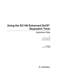
Figure 3-1 illustrates these tasks.
Start
Write C code with
higher ILP potential
Compile and
analyze the
generated
assembly code
Is the
result
satisfactory?
Compiler
achieves the
required ILP
for the given
C code
Based on the analysis, change the
way of writing (so the compiler
may generate better code)
NO
YES
End
Figure 3-1. Optimized C General Workflow
3-1
For More Information On This Product,
Go to: www.freescale.com
Freescale Semiconductor, Inc.
Structured C Approach to Application Development
3.2 Studying Test Cases
Freescale Semiconductor, Inc...
This section presents test cases that illustrate the techniques of writing structured C code. The test cases
are taken from the standard C description of the GSM EFR vocoder. For each test case, the standard C
code and an evolutionary track towards a structured C version are presented. The code is compiled in a
separate mode (each module is compiled alone) using switch Ot2 for speed optimization. The test cases
presented are :
• Vq_subvec_s. Performs vector quantization, using distances between vectors, as described in Section
3.2.1.
• Lag_max. Determines the maximum correlation between an input signal and the same signal with a
delay, within a range of input signal delays, as described in Section 3.2.2.
• Norm_Corr. Determines the normalized correlation between a target vector and the filtered past
excitation, as described in Section 3.2.3.
3.2.1 Vq_subvec_s Test Case
The Vq_subvec_s function performs vector quantization. The distance (weighted Euclidean norm) is
computed for an input with a four element vector from a vector in a fixed codebook. The vector with the
minimum distance to the input vector is used to represent it. Actually, the input vector is compared with a
vector from the codebook and with the same vector with the opposite direction.
index of nearest vector = arg { min { V – V i } }
i
3
where V – V i =
∑ [ W ( k ) ⋅ ( V( k ) – Vi ( k ) ) ]
2
k=0
The standard C code is as follows:
/* Quantization of a 4 dimensional subvector with a signed codebook */
Word16 Vq_subvec_s (/* output: return quantization index
*/
Word16 *lsf_r1,/* input : 1st LSF residual vector
*/
Word16 *lsf_r2,/* input : 2nd LSF residual vector
*/
const Word16 *dico,/* input : quantization codebook
*/
Word16 *wf1,/* input : 1st LSF weighting factors
*/
Word16 *wf2,/* input : 2nd LSF weighting factors
*/
Word16 dico_size)/* input : size of quantization codebook */
{
Word16 i, index, sign, temp;
const Word16 *p_dico;
Word32 dist_min, dist;
dist_min = MAX_32;
p_dico = dico;
for (i = 0; i < dico_size; i++)
{
/* test positive */
temp = sub (lsf_r1[0], *p_dico++);
temp = mult (wf1[0], temp);
dist = L_mult (temp, temp);
temp = sub (lsf_r1[1], *p_dico++);
temp = mult (wf1[1], temp);
dist = L_mac (dist, temp, temp);
temp = sub (lsf_r2[0], *p_dico++);
3-2
For More Information On This Product,
Go to: www.freescale.com
Freescale Semiconductor, Inc.
Structured C Approach to Application Development
temp = mult (wf2[0], temp);
dist = L_mac (dist, temp, temp);
temp = sub (lsf_r2[1], *p_dico++);
temp = mult (wf2[1], temp);
dist = L_mac (dist, temp, temp);
Freescale Semiconductor, Inc...
if (L_sub (dist, dist_min) < (Word32) 0)
{
dist_min = dist;
index = i;
sign = 0;
}
/* test negative */
p_dico
temp =
temp =
dist =
-= 4;
add (lsf_r1[0], *p_dico++);
mult (wf1[0], temp);
L_mult (temp, temp);
temp = add (lsf_r1[1], *p_dico++);
temp = mult (wf1[1], temp);
dist = L_mac (dist, temp, temp);
temp = add (lsf_r2[0], *p_dico++);
temp = mult (wf2[0], temp);
dist = L_mac (dist, temp, temp);
temp = add (lsf_r2[1], *p_dico++);
temp = mult (wf2[1], temp);
dist = L_mac (dist, temp, temp);
if (L_sub (dist, dist_min) < (Word32) 0)
{
dist_min = dist;
index = i;
sign = 1;
}
}
/* Reading the selected vector */
p_dico = &dico[shl (index, 2)];
if (sign == 0)
{
lsf_r1[0] =
lsf_r1[1] =
lsf_r2[0] =
lsf_r2[1] =
}
else
{
lsf_r1[0] =
lsf_r1[1] =
lsf_r2[0] =
lsf_r2[1] =
}
*p_dico++;
*p_dico++;
*p_dico++;
*p_dico++;
negate
negate
negate
negate
(*p_dico++);
(*p_dico++);
(*p_dico++);
(*p_dico++);
index = shl (index, 1);
index = add (index, sign);
return index;
3-3
For More Information On This Product,
Go to: www.freescale.com
Freescale Semiconductor, Inc.
Structured C Approach to Application Development
The structured C code shown is the following sections is described step-by-step. An explanation is
provided for the impact of each step on the produced code.
Note:
The altered code is shown in bold.
Freescale Semiconductor, Inc...
A loop in the code typically consumes the most processing cycles. Each loop iteration, as shown in the
preceding code, contains two distance calculations followed by a comparison and update, if necessary.
This C code shows high ILP potential.
In principle, the two distances, positive and negative cases, can be calculated concurrently. The
calculations that are accumulated to the distance measure can also be computed concurrently to provide
further ILP. Using bound calculations from index [2] shows that the minimum loop length is seven
execution sets. The assembly code for this loop contains few points of access to the stack. These are
directly linked to the two variables index and sign. In the update phase (after comparison), these two
variables are stored in two DALU registers. The compiler needs these registers later, for calculations, and
spills them to the stack. The spill code, such as iff moves.f d11,(sp-44), takes two cycles to
execute if the true bit is set to off (that is, an update is needed and probably occurs, but a relatively small
number of times). It takes one cycle to execute if the true bit is set to on (that is, no update is required,
probably the situation for most cases). We recommend that you avoid, where possible, a code with a spill
to stack, as defined in loops.
3.2.1.1 Vq_subvec_s—The First Step
The following code shows the first step towards more efficient compiled C code:
Word16 Vq_subvec_s (
/* output: return quantization index
Word16 *lsf_r1,
/* input : 1st LSF residual vector
Word16 *lsf_r2,
/* input : 2nd LSF residual vector
const Word16 *dico, /* input : quantization codebook
Word16 *wf1,
/* input : 1st LSF weighting factors
Word16 *wf2,
/* input : 2nd LSF weighting factors
Word16 dico_size)
/* input : size of quantization codebook
{
Word16 i, index, sign, temp;
const Word16 *p_dico;
Word32 dist_min, dist;
Word16 temp16_1, temp16_2, temp16_3, temp16_4;
dist_min = MAX_32;
p_dico = dico;
for (i = 1; i < dico_size+1; i++)
{
/* test positive */
temp = sub (lsf_r1[0], *p_dico++);
temp = mult (wf1[0], temp);
dist = L_mult (temp, temp);
temp = sub (lsf_r1[1], *p_dico++);
temp = mult (wf1[1], temp);
dist = L_mac (dist, temp, temp);
temp = sub (lsf_r2[0], *p_dico++);
temp = mult (wf2[0], temp);
dist = L_mac (dist, temp, temp);
temp = sub (lsf_r2[1], *p_dico++);
temp = mult (wf2[1], temp);
dist = L_mac (dist, temp, temp);
3-4
For More Information On This Product,
Go to: www.freescale.com
*/
*/
*/
*/
*/
*/
*/
Freescale Semiconductor, Inc.
Structured C Approach to Application Development
if (L_sub (dist, dist_min) < (Word32) 0)
{
dist_min = dist;
index = i;
}
/* test negative */
p_dico
temp =
temp =
dist =
-= 4;
add (lsf_r1[0], *p_dico++);
mult (wf1[0], temp);
L_mult (temp, temp);
Freescale Semiconductor, Inc...
temp = add (lsf_r1[1], *p_dico++);
temp = mult (wf1[1], temp);
dist = L_mac (dist, temp, temp);
temp = add (lsf_r2[0], *p_dico++);
temp = mult (wf2[0], temp);
dist = L_mac (dist, temp, temp);
temp = add (lsf_r2[1], *p_dico++);
temp = mult (wf2[1], temp);
dist = L_mac (dist, temp, temp);
if (L_sub (dist, dist_min) < (Word32) 0)
{
dist_min = dist;
index = negate (i);
}
}
/* Extracting sign and index true values */
sign = 0;
if ( index < 0 )
{
sign = 1;
index = negate (index);
}
index = sub (index, 1);
/* Reading the selected vector */
p_dico = &dico[shl (index, 2)];
temp16_1
temp16_2
temp16_3
temp16_4
=
=
=
=
p_dico[0];
p_dico[1];
p_dico[2];
p_dico[3];
if (sign ==
{
temp16_1
temp16_2
temp16_3
temp16_4
}
1)
lsf_r1[0]
lsf_r1[1]
lsf_r2[0]
lsf_r2[1]
temp16_1;
temp16_2;
temp16_3;
temp16_4;
=
=
=
=
=
=
=
=
negate
negate
negate
negate
(temp16_1);
(temp16_2);
(temp16_3);
(temp16_4);
index = shl (index, 1);
index = add (index, sign);
3-5
For More Information On This Product,
Go to: www.freescale.com
Freescale Semiconductor, Inc.
Structured C Approach to Application Development
return index;
Freescale Semiconductor, Inc...
To avoid the spill code in the loop, we eliminate the variable sign from the loop and including the sign
information in the index. For the positive case (sign = 0), index is updated with i, which is always
positive. For the negative case (sign = 1), index is updated with the negated value, meaning the value that
is always negative. To avoid the case of zero, i is preset to a value of one. After the loop, the true values
of sign and index are restored. This change reduces the spill code. For the standard code, the loop has
23 execution sets with four accesses to stack. For the structured code, the loop has only 20 execution sets
with two access to stack. We also change how the selected vector is read (after the loop), as follows:
1.
The vector is read from the codebook into temporary variables (temp16_1, temp16_2, temp16_3,
and temp16_4).
2.
According to the sign, the values of these variables are updated.
3.
Variables are stored to lsf_r1 and lsf_r2.
This code size is improved over the standard code because the vector is read only once from the
codebook and lsf_r1 and lsf_r2 are written only once. However, for the standard code, there are two
segments of code that read the vector from codebook: one for the case sign is zero and the other for the
case sign is one. In addition, there remains two segments of code to write to lsf_r1 and lsf_r2 for
both cases.
3.2.1.2 Vq_subvec_s—The Second Step
The second towards more efficient code eliminates the remaining spill code in the loop.
Word16 Vq_subvec_s (
/* output: return quantization index
Word16 *lsf_r1,
/* input : 1st LSF residual vector
Word16 *lsf_r2,
/* input : 2nd LSF residual vector
const Word16 *dico, /* input : quantization codebook
Word16 *wf1,
/* input : 1st LSF weighting factors
Word16 *wf2,
/* input : 2nd LSF weighting factors
Word16 dico_size)
/* input : size of quantization codebook
{
Word16 i, index, sign, temp;
const Word16 *p_dico;
Word32 dist_min, dist;
Word16 *indexAGU, tem[2], *j, *j_negate;
Word16 temp16_1, temp16_2, temp16_3, temp16_4;
*/
*/
*/
*/
*/
*/
*/
dist_min = MAX_32;
indexAGU = &tem[0]; /*
This has been done to avoid the stack-related
addressing (sp-offset) which takes two cycles.
The indexAGU is allocated to the AGU register.
Therefore, two DALU registers are freed.
j = indexAGU;
j_negate = indexAGU;
p_dico = dico;
for (i = 0; i < dico_size; i++)
{
/* test positive */
temp = sub (lsf_r1[0], *p_dico++);
temp = mult (wf1[0], temp);
dist = L_mult (temp, temp);
temp = sub (lsf_r1[1], *p_dico++);
temp = mult (wf1[1], temp);
dist = L_mac (dist, temp, temp);
3-6
For More Information On This Product,
Go to: www.freescale.com
*/
Freescale Semiconductor, Inc.
Structured C Approach to Application Development
temp = sub (lsf_r2[0], *p_dico++);
temp = mult (wf2[0], temp);
dist = L_mac (dist, temp, temp);
temp = sub (lsf_r2[1], *p_dico++);
temp = mult (wf2[1], temp);
dist = L_mac (dist, temp, temp);
Freescale Semiconductor, Inc...
j++;
if (L_sub (dist, dist_min) < (Word32) 0)
{
dist_min = dist;
indexAGU = j;
}
/* test negative */
p_dico
temp =
temp =
dist =
-= 4;
add (lsf_r1[0], *p_dico++);
mult (wf1[0], temp);
L_mult (temp, temp);
temp = add (lsf_r1[1], *p_dico++);
temp = mult (wf1[1], temp);
dist = L_mac (dist, temp, temp);
temp = add (lsf_r2[0], *p_dico++);
temp = mult (wf2[0], temp);
dist = L_mac (dist, temp, temp);
temp = add (lsf_r2[1], *p_dico++);
temp = mult (wf2[1], temp);
dist = L_mac (dist, temp, temp);
j_negate--;
if (L_sub (dist, dist_min) < (Word32) 0)
{
dist_min = dist;
indexAGU = j_negate;
}
}
/* Extracting the sign and index true values */
index = indexAGU - &tem[0];
sign = 0;
if ( index < 0 )
{
sign = 1;
index = negate (index);
}
index = sub (index, 1);
/* Reading the selected vector */
p_dico = &dico[shl (index, 2)];
temp16_1
temp16_2
temp16_3
temp16_4
=
=
=
=
if (sign ==
{
temp16_1
temp16_2
temp16_3
temp16_4
p_dico[0];
p_dico[1];
p_dico[2];
p_dico[3];
1)
=
=
=
=
negate
negate
negate
negate
(temp16_1);
(temp16_2);
(temp16_3);
(temp16_4);
3-7
For More Information On This Product,
Go to: www.freescale.com
Freescale Semiconductor, Inc.
Structured C Approach to Application Development
}
lsf_r1[0]
lsf_r1[1]
lsf_r2[0]
lsf_r2[1]
=
=
=
=
temp16_1;
temp16_2;
temp16_3;
temp16_4;
index = shl (index, 1);
index = add (index, sign);
Freescale Semiconductor, Inc...
return index;
The spill code in the loop (linked to the variable index of the former code) is eliminated by allocating
index to an AGU register. A variable indexAGU is declared to be of the type: pointer to Word16. This
variable replaces the index role in the loop. Once the index is stored in an AGU register, the operations
index = i and index = negate (i) are replaced by an AGU operation. Two Word16 pointers, j and
j_negate, are defined and initialized to point to a dummy location &tem[0].
During the loop, j is increased by j++ operation (it is compiled to an AGU add operation). j_negate
is decreased by j_negate-- operation (it is also compiled to an AGU add operation). The index update is
performed by indexAGU = j or indexAGU = j_negate, which are AGU operations. As before,
index and sign are restorable from indexAGU. Loop length is reduced to 18 execution sets without
stack access (however, the code size increases slightly by 24 bytes).
The statement:
if (L_sub (dist, dist_min) < (Word32) 0)
is replaced with:
if ( dist < dist_min )
The sub operation is saved and the statement occurs twice in the loop. Loop length is reduced to 16
execution sets.
3.2.1.3 Vq_subvec_s—The Third Step
The next step is to try to increase the speed of the code. Observing the generated assembly code for the
loop shows that access to the codebook is through one pointer (r5). Therefore, the calculation of the
distance for the negative case cannot start before the first element from the codebook is loaded. The
compiler does not recognize that it is also the first element needed for the calculation of the distance for
the positive case. Therefore, the first element for the negative case is loaded after the last element for the
positive case is loaded. The following code tells the compiler that vector elements for the negative case
are the same elements as for the positive case. In this step, the following shows the code of the loop (the
rest is not changed):
for (i = 0; i < dico_size; i++, p_dico+=4)
{
/* test positive */
temp = sub (lsf_r1[0], p_dico[0]);
temp = mult (wf1[0], temp);
dist = L_mult (temp, temp);
temp = sub (lsf_r1[1], p_dico[1]);
temp = mult (wf1[1], temp);
dist = L_mac (dist, temp, temp);
temp = sub (lsf_r2[0], p_dico[2]);
temp = mult (wf2[0], temp);
dist = L_mac (dist, temp, temp);
temp = sub (lsf_r2[1], p_dico[3]);
3-8
For More Information On This Product,
Go to: www.freescale.com
Freescale Semiconductor, Inc.
Structured C Approach to Application Development
temp = mult (wf2[1], temp);
dist = L_mac (dist, temp, temp);
j++;
if ( dist < dist_min )
{
dist_min = dist;
indexAGU = j;
}
/* test negative */
Freescale Semiconductor, Inc...
temp = add (lsf_r1[0], p_dico[0]);
temp = mult (wf1[0], temp);
dist = L_mult (temp, temp);
temp = add (lsf_r1[1], p_dico[1]);
temp = mult (wf1[1], temp);
dist = L_mac (dist, temp, temp);
temp = add (lsf_r2[0], p_dico[2]);
temp = mult (wf2[0], temp);
dist = L_mac (dist, temp, temp);
temp = add (lsf_r2[1], p_dico[3]);
temp = mult (wf2[1], temp);
dist = L_mac (dist, temp, temp);
j_negate--;
if ( dist < dist_min )
{
dist_min = dist;
indexAGU = j_negate;
}
}
Access to codebook elements occurs through p_dico[k]. The corresponding generated assembly code
loads each element from the codebook only once (and not twice as before). In addition, it calculates the
distances in parallel for the positive case and negative case. However, the loop length decreases by only
one execution set to a total of 15 execution sets.
This unsatisfying result is based on the compiler using the same register to hold the values for both
distances, positive and negative cases. In other words, all calculations that do not assign a value to dist
in the negative case occur in parallel with distance calculations for the positive case. However, all
assignments to dist in the negative case begin only after the distance of the positive case is used for
comparison and update. The following code overcomes this problem:
for (i = 0; i < dico_size; i++, p_dico+=4)
{
/* compute positive */
temp = sub (lsf_r1[0], p_dico[0]);
temp = mult (wf1[0], temp);
dist = L_mult (temp, temp);
temp = sub (lsf_r1[1], p_dico[1]);
temp = mult (wf1[1], temp);
dist = L_mac (dist, temp, temp);
temp = sub (lsf_r2[0], p_dico[2]);
temp = mult (wf2[0], temp);
dist = L_mac (dist, temp, temp);
temp = sub (lsf_r2[1], p_dico[3]);
temp = mult (wf2[1], temp);
dist = L_mac (dist, temp, temp);
3-9
For More Information On This Product,
Go to: www.freescale.com
Freescale Semiconductor, Inc.
Structured C Approach to Application Development
/* compute negative */
temp = add (lsf_r1[0], p_dico[0]);
temp = mult (wf1[0], temp);
dist1 = L_mult (temp, temp);
temp = add (lsf_r1[1], p_dico[1]);
temp = mult (wf1[1], temp);
dist1 = L_mac (dist1, temp, temp);
temp = add (lsf_r2[0], p_dico[2]);
temp = mult (wf2[0], temp);
dist1 = L_mac (dist1, temp, temp);
Freescale Semiconductor, Inc...
temp = add (lsf_r2[1], p_dico[3]);
temp = mult (wf2[1], temp);
dist1 = L_mac (dist1, temp, temp);
/* test positive */
j++;
if ( dist < dist_min )
{
dist_min = dist;
indexAGU = j;
}
/* test negative */
j_negate--;
if ( dist1 < dist_min )
{
dist_min = dist1;
indexAGU = j_negate;
}
}
Two changes were made:
1.
The distances for the negative and positive cases are stored in different variables (positive case in
dist, negative case in dist1).
2.
The code that calculates dist1 is moved before the compare and select statement of the positive case.
The loop length is reduced by three to a total of 12 execution sets.
3.2.1.4 Vq_subvec_s—The Fourth Step
The compiler does not pipeline the calculations in the loop (meaning that it does not begin operations of
the next iteration in the current iteration). If pipelineing or split-summation are not used for calculating
dist then, dist is ready only at the eighth execution unit. Therefore, the comparison of dist1 to
dist_min cannot be before the tenth execution set, which means that all loops can take no less then 12
execution sets. Remember, indexAGU is stored in an AGU register, and due to processor pipeline latency,
its update can occur at least one cycle after the TRUE bit is written. The compiler achieves this result.
To reduce loop length further, we use a pipelineing technique. For example, if p_dico[0] for the next
iteration is loaded at the current iteration, then loop length can reduce to 11 execution sets. The code for
this last stage, is as follows:
temp16_1 = p_dico[0];
for (i = 0; i < dico_size; i++, p_dico+=4)
{
/* test positive */
temp = sub (lsf_r1[0], temp16_1);
temp = mult (wf1[0], temp);
dist = L_mult (temp, temp);
3-10
For More Information On This Product,
Go to: www.freescale.com
Freescale Semiconductor, Inc.
Structured C Approach to Application Development
temp = sub (lsf_r1[1], p_dico[1]);
temp = mult (wf1[1], temp);
dist = L_mac (dist, temp, temp);
temp = sub (lsf_r2[0], p_dico[2]);
temp = mult (wf2[0], temp);
dist = L_mac (dist, temp, temp);
Freescale Semiconductor, Inc...
temp = sub (lsf_r2[1], p_dico[3]);
temp = mult (wf2[1], temp);
dist = L_mac (dist, temp, temp);
temp = add (lsf_r1[0], temp16_1);
temp = mult (wf1[0], temp);
dist1 = L_mult (temp, temp);
temp = add (lsf_r1[1], p_dico[1]);
temp = mult (wf1[1], temp);
dist1 = L_mac (dist1, temp, temp);
temp = add (lsf_r2[0], p_dico[2]);
temp = mult (wf2[0], temp);
dist1 = L_mac (dist1, temp, temp);
temp = add (lsf_r2[1], p_dico[3]);
temp = mult (wf2[1], temp);
dist1 = L_mac (dist1, temp, temp);
j++;
if ( dist < dist_min )
{
dist_min = dist;
indexAGU = j;
}
/* test negative */
j_negate--;
if ( dist1 < dist_min )
{
dist_min = dist1;
indexAGU = j_negate;
}
temp16_1 = p_dico[4];
}
Before the first iteration, p_dico[0] is loaded into temp16_1. Therefore, dist calculation begins at the
first execution set. At the end of the current iteration, p_dico[0] of the next iteration is loaded to
temp16_1 (temp16_1 = p_dico[4]). Loop length is now 11 execution units.
3.2.1.5 Vq_subvec_s—Example Summary
In the initial C code, each loop iteration requires at least 23 cycles. In the final C code, each loop iteration
requires 11 cycles. The initial C Code of the loop had high ILP potential, but the compiler failed to
deliver high ILP machine code, so the C code was rewritten. The number of variables in the loop,
assigned to DALU registers, is reduced by eliminating a variable and assigning a variable to an AGU
register.
3-11
For More Information On This Product,
Go to: www.freescale.com
Freescale Semiconductor, Inc.
Structured C Approach to Application Development
A statement with two operations was transformed to a statement with one equivalent operation. Direct
access to the array is replaced by indirect access to the array. A code segment in the loop has moved and
as a result, another variable is defined. This results in pipelining the load operation and reducing the code
size from 464 bytes to 428 bytes.
3.2.2 Lag_max Test Case
Another code example uses the Lag_max function. We next evaluate how to optimize its performance.
This function is part of the open loop pitch search. It computes the correlation of the input signal with the
same signal delayed, for a range of delays. The function finds the delay with the maximum correlation
and returns the delay with its correlation value after normalization.
The standard C code, is as follows:
Freescale Semiconductor, Inc...
#include "prototype.h"
#include "oper_32b.h"
#include "sig_proc.h"
#define THRESHOLD 27853
/*************************************************************************
*
* FUNCTION: Lag_max
*
*
*
*
*
*
*
PURPOSE: Find the lag that has the maximum correlation of scal_sig[] in a
given delay range.
DESCRIPTION:
The correlation is given by
cor[t] = <scal_sig[n],scal_sig[n-t]>,
t=lag_min,...,lag_max
* The function output is the maximum correlation after normalization
*
and the corresponding lag.
*
*************************************************************************/
Word16 Lag_max (
/* output: lag found */
Word16 scal_sig[], /* input : scaled signal */
Word16 scal_fac,
/* input : scaled signal factor */
Word16 L_frame,
/* input : length of the frame to compute the pitch*/
Word16 lag_max,
/* input : maximum lag
*/
Word16 lag_min,
/* input : minimum lag
*/
Word16 *cor_max)
/* output: normalized correlation of selected lag */
{
Word16 i, j;
Word16 *p, *p1;
Word32 max, t0;
Word16 max_h, max_l, ener_h, ener_l;
Word16 p_max;
max = MIN_32;
for (i = lag_max; i >= lag_min; i--)
{
p = scal_sig;
p1 = &scal_sig[-i];
t0 = 0;
for (j = 0; j < L_frame; j++, p++, p1++)
{
t0 = L_mac (t0, *p, *p1);
}
if (L_sub (t0, max) >= 0)
3-12
For More Information On This Product,
Go to: www.freescale.com
Freescale Semiconductor, Inc.
Structured C Approach to Application Development
{
max = t0;
p_max = i;
}
}
/* compute energy */
Freescale Semiconductor, Inc...
t0 = 0;
p = &scal_sig[-p_max];
for (i = 0; i < L_frame; i++, p++)
{
t0 = L_mac (t0, *p, *p);
}
/* 1/sqrt(energy) */
t0 = Inv_sqrt (t0);
t0 = L_shl (t0, 1);
/* max = max/sqrt(energy)
*/
L_Extract (max, &max_h, &max_l);
L_Extract (t0, &ener_h, &ener_l);
t0 = Mpy_32 (max_h, max_l, ener_h, ener_l);
t0 = L_shr (t0, scal_fac);
*cor_max = extract_h (L_shl (t0, 15));
/* divide by 2 */
return (p_max);
}
The most consuming cycle count part is the following:
for (j = 0; j < L_frame; j++, p++, p1++)
{
t0 = L_mac (t0, *p, *p1);
}
This code has low ILP. It was compiled to a loop with one execution set that uses only one MAC unit. For
better speed, this code must be transformed into code with a higher ILP potential. The correlation
calculation is compatible with multisample processing, which can reduce cycle count for the SC140 core
by as much as a factor of four, relative to single sample processing.
Word16 Lag_max (
/* output: lag found
Word16 scal_sig[], /* input : scaled signal.
Word16 scal_fac,
/* input : scaled signal factor.
Word16 lag_max,
/* input : maximum lag
Word16 lag_min,
/* input : minimum lag
Word16 *cor_max)
/* output: normalized correlation of selected lag
{
Word16 i, j, k;
Word16 *p, *p1;
Word32 max, t0, t1, t2, t3;
Word16 max_h, max_l, ener_h, ener_l;
Word16 p_max;
Word32 Corr_local[72];
*/
*/
*/
*/
*/
*/
max = MIN_32;
#define L_frame 80 /*length of frame to compute the pitch*/
/* Calculate correlations and store in a temporary array */
for (i = lag_max, k = 0; i >= lag_min; i-=4, k+=4)
{
p = scal_sig;
p1 = &scal_sig[-i];
3-13
For More Information On This Product,
Go to: www.freescale.com
Freescale Semiconductor, Inc.
Structured C Approach to Application Development
t0 = 0; t1 = 0; t2 = 0; t3 = 0;
for (j
{
t0
t1
t2
t3
}
= 0; j < L_frame; j++, p++, p1++)
=
=
=
=
L_mac
L_mac
L_mac
L_mac
(t0,
(t1,
(t2,
(t3,
Corr_local[k+0]
Corr_local[k+1]
Corr_local[k+2]
Corr_local[k+3]
=
=
=
=
*p,
*p,
*p,
*p,
p1[0]);
p1[1]);
p1[2]);
p1[3]);
t0;
t1;
t2;
t3;
}
Freescale Semiconductor, Inc...
/* Scan the temporary array to find the largest correlation and its index */
p_max = 0;
for (i = lag_max, j=0; i >= lag_min; i--, j++)
{
if ( Corr_local[j] >= max )
{
max = Corr_local[j];
p_max = i;
}
}
/* compute energy */
t0 = 0;
p = &scal_sig[-p_max];
for (i = 0; i < L_frame; i++, p++)
{
t0 = L_mac (t0, *p, *p);
}
/* 1/sqrt(energy) */
t0 = Inv_sqrt (t0);
t0 = L_shl (t0, 1);
/* max = max/sqrt(energy)
*/
L_Extract (max, &max_h, &max_l);
L_Extract (t0, &ener_h, &ener_l);
t0 = Mpy_32 (max_h, max_l, ener_h, ener_l);
t0 = L_shr (t0, scal_fac);
*cor_max = extract_h (L_shl (t0, 15));
/* divide by 2 */
return (p_max);
}
To apply multisample processing of quad samples, some changes are required. In each call to this
function, lag_max-lag_min+1 correlations are computed. According to the EFR standard, this number
can be one of three: 72, 36, or 18. To write compact code that handles the three cases uniformly, (the
problematic case is 18 because it is not a multiple of four), the calculation of correlations is separated
from the compare/select operations, as follows:
1.
The correlations are computed and stored in a temporary array (for the case of 18 correlations two
more correlations are calculated).
2.
The temporary array is scanned and the largest correlation and its index are found (for the 18 case, the
extra two calculated correlations are ignored).
3-14
For More Information On This Product,
Go to: www.freescale.com
Freescale Semiconductor, Inc.
Structured C Approach to Application Development
Observing the code that the compiler generates for the multisample code shows that the compiler does
not improve the machine code ILP. Still, in each execution set (in the correlations calculation loop) only
one MAC is used. The key reason for this is that the compiler does not recognize that p1[0], p1[1],
and p1[2] of the current iteration are actually p1[1], p1[2] and p1[3], respectively, of the
previous iteration. In the code that we show next, we pass this information to the compiler.
Two more changes are made. The passed parameter L_frame is always the same, so it is not passed and
is hard coded.
The following statement:
if (L_sub (t0, max) >= 0)
is replaced with:
Freescale Semiconductor, Inc...
if ( Corr_local[j] >= max )
The L_sub is eliminated and replaced by a proper relation operator. The code of the multisample loop is
rewritten, as follows (the rest remains the same):
{ Word16 temp16_1, temp16_2, temp16_3;
temp16_1 = *p1++;
temp16_2 = *p1++;
temp16_3 = *p1++;
for (j
{
t0
t1
t2
t3
= 0; j < L_frame; j++, p++)
=
=
=
=
L_mac
L_mac
L_mac
L_mac
(t0,
(t1,
(t2,
(t3,
*p,
*p,
*p,
*p,
temp16_1);
temp16_2);
temp16_3);
*p1);
/* For next iteration */
temp16_1 = temp16_2;
temp16_2 = temp16_3;
temp16_3 = *p1++;
}
}
The loop is compiled to a machine code with two execution sets that contain a total of four MAC
operations and three TFR operations. The machine code ILP is improved, but not sufficiently, because the
three TFR operations are merely for reuse of the operands. This can be improved by writing the loop
differently, by reducing the loop count and increasing the number of operations performed in each
iteration, as shown here:
{ Word16 temp16_1, temp16_2, temp16_3, temp16_4;
temp16_1
temp16_2
temp16_3
temp16_4
=
=
=
=
*p1++;
*p1++;
*p1++;
*p1++;
for (j = 0; j < L_frame; j+=4)
{
t0 = L_mac (t0, *p, temp16_1);
t1 = L_mac (t1, *p, temp16_2);
t2 = L_mac (t2, *p, temp16_3);
t3 = L_mac (t3, *p, temp16_4);
p++;
temp16_1 = *p1++;
t0 =
t1 =
t2 =
t3 =
p++;
L_mac
L_mac
L_mac
L_mac
(t0,
(t1,
(t2,
(t3,
*p,
*p,
*p,
*p,
temp16_2);
temp16_3);
temp16_4);
temp16_1);
3-15
For More Information On This Product,
Go to: www.freescale.com
Freescale Semiconductor, Inc.
Structured C Approach to Application Development
temp16_2 = *p1++;
t0 = L_mac
t1 = L_mac
t2 = L_mac
t3 = L_mac
p++;
temp16_3 =
(t0,
(t1,
(t2,
(t3,
t0 = L_mac
t1 = L_mac
t2 = L_mac
t3 = L_mac
p++;
temp16_4 =
(t0,
(t1,
(t2,
(t3,
*p,
*p,
*p,
*p,
temp16_3);
temp16_4);
temp16_1);
temp16_2);
*p1++;
*p,
*p,
*p,
*p,
temp16_4);
temp16_1);
temp16_2);
temp16_3);
*p1++;
Freescale Semiconductor, Inc...
}
}
This code achieves the highest ILP. The loop has four execution sets, with four MAC operations executed
in each set. The compiler is explicitly directed how to reuse operands (with no need to TFR operands).
The original loop count is, L_frame, which is 80. Fortunately, this is a multiple of 4, so the new loop
count is L_frame/4=20. If L_frame is not a multiple of four, the code must be changed further.
For a possible solution, scal_sig[0] to scal_sig[L_frame-1] can be copied to a temporary array
that is padded with zeros at the end, p initialization: p = temp_array;, and the loop count is
x=ceill(L_frame/4), meaning that 4*x is the smallest number that is greater than or equal to
L_frame.
In the initial C code, the main kernel has low ILP potential, so it is compiled to one execution set that
exercises only one MAC unit. In the final C code the main kernel has high ILP potential and it is
compiled to four execution sets, in which all four MAC units are in use (maximum utilization) in each
execution set. The initial low-level potential C code is transformed to code with higher ILP potential by
using multisample processing to process four samples concurrently.
To reuse operands loaded from memory without using TFR operations, the loop is expended to contain
four accumulations for each sample. To have a uniform compact code for the range of passed arguments,
the correlation calculation is separated from choosing the maximum correlation operation. In principle,
the main kernel in the final code runs four times faster than the main kernel in the initial code (code size
increases from 362 bytes to 596 bytes).
3.2.3 Norm_Corr Test Case
The Norm_Corr function finds the normalized correlation between the target vector and the filtered past
excitation. In this example, techniques not used before are applied.
The standard C code is shown, with one slight change. Originally L_subfr was passed as a parameter.
Since it always has the same value, it can be replaced by a constant.
#include
#include
#include
#include
"prototype.h"
"oper_32b.h"
"sig_proc.h"
"codec.h"
/* L_inter = Length for fractional interpolation = nb.coeff/2 */
#define L_inter 4
/*************************************************************************
*
* FUNCTION:
Norm_Corr()
*
* PURPOSE: Find the normalized correlation between the target vector
3-16
For More Information On This Product,
Go to: www.freescale.com
Freescale Semiconductor, Inc.
Structured C Approach to Application Development
Freescale Semiconductor, Inc...
*
and the filtered past excitation.
*
* DESCRIPTION:
*
The normalized correlation is given by the correlation between the
*
target and filtered past excitation divided by the square root of
*
the energy of filtered excitation.
*
corr[k] = <x[], y_k[]>/sqrt(y_k[],y_k[])
*
where x[] is the target vector and y_k[] is the filtered past
*
excitation at delay k.
*
*************************************************************************/
void Norm_Corr (Word16 exc[], Word16 xn[], Word16 h[],
Word16 t_min, Word16 t_max, Word16 corr_norm[])
{
Word16 i, j, k;
Word16 corr_h, corr_l, norm_h, norm_l;
Word32 s;
/* Usally dynamic allocation of (L_subfr) */
Word16 excf[80];
Word16 scaling, h_fac, *s_excf, scaled_excf[80];
#define L_subfr 40
k = -t_min;
/* compute the filtered excitation for the first delay t_min */
Convolve (&exc[k], h, excf, L_subfr);
/* scale "excf[]" to avoid overflow */
for (j = 0; j < L_subfr; j++)
{
scaled_excf[j] = shr (excf[j], 2);
}
/* Compute 1/sqrt(energy of excf[]) */
s = 0;
for (j = 0; j < L_subfr; j++)
{
s = L_mac (s, excf[j], excf[j]);
}
if (L_sub (s, 67108864L) <= 0)
{
s_excf = excf;
h_fac = 15 - 12;
scaling = 0;
}
else
{
/* "excf[]" is divided by 2 */
s_excf = scaled_excf;
h_fac = 15 - 12 - 2;
scaling = 2;
}
/* if (s <= 2^26) */
/* loop for each possible period */
for (i = t_min; i <= t_max; i++)
{
/* Compute 1/sqrt(energy of excf[]) */
s = 0;
for (j = 0; j < L_subfr; j++)
{
3-17
For More Information On This Product,
Go to: www.freescale.com
Freescale Semiconductor, Inc.
Structured C Approach to Application Development
s = L_mac (s, s_excf[j], s_excf[j]);
}
s = Inv_sqrt (s);
L_Extract (s, &norm_h, &norm_l);
/* Compute the correlation between xn[] and excf[] */
s = 0;
for (j = 0; j < L_subfr; j++)
{
s = L_mac (s, xn[j], s_excf[j]);
}
L_Extract (s, &corr_h, &corr_l);
Freescale Semiconductor, Inc...
/* Normalize correlation = correlation * (1/sqrt(energy)) */
s = Mpy_32 (corr_h, corr_l, norm_h, norm_l);
corr_norm[i] = extract_h (L_shl (s, 16));
/* modify the filtered excitation excf[] for the next iteration */
if (sub (i, t_max) != 0)
{
k--;
for (j = L_subfr - 1; j > 0; j--)
{
s = L_mult (exc[k], h[j]);
s = L_shl (s, h_fac);
s_excf[j] = add (extract_h (s), s_excf[j - 1]);
}
s_excf[0] = shr (exc[k], scaling);
}
}
return;
}
We start by analyzing the code generated for the following C code:
/* scale "excf[]" to avoid overflow */
for (j = 0; j < L_subfr; j++)
{
scaled_excf[j] = shr (excf[j], 2);
}
Although this C code does not consume many cycles, it is a good example with low ILP potential. The
compiler-produced code has three execution sets, so the machine code has low ILP. If arrays excf and
scaled_excf are aligned to eight (the array base address is a multiply of eight, with four elements that
can be loaded in one load operation), then four elements can be processed in parallel. Since these two
arrays are local to this function, using a pragma align guarantees that they are aligned as eight.
The structured code is as follows:
#pragma align excf
8
#pragma align scaled_excf 8
/* scale "excf[]" to avoid overflow */
for (j = 0; j < L_subfr; j+=4)
{
scaled_excf[j+0] = shr (excf[j+0],
scaled_excf[j+1] = shr (excf[j+1],
scaled_excf[j+2] = shr (excf[j+2],
scaled_excf[j+3] = shr (excf[j+3],
2);
2);
2);
2);
3-18
For More Information On This Product,
Go to: www.freescale.com
Freescale Semiconductor, Inc.
Structured C Approach to Application Development
}
This loop also has three execution sets, but it processes four samples in each iteration (the number of
iterations is reduced from 40 to 10). However, it can have higher machine code ILP if the loop is
pipelined (only two execution sets). The compiler does not pipeline the loop. Instead, the following code
tries to do it:
Freescale Semiconductor, Inc...
/* scale "excf[]" to avoid overflow */
{ Word16 temp16_1, temp16_2, temp16_3, temp16_4;
temp16_1 = excf[0];
temp16_2 = excf[1];
temp16_3 = excf[2];
temp16_4 = excf[3];
for (j = 0; j < L_subfr; j+=4)
{
temp16_1 = shr (temp16_1, 2);
temp16_2 = shr (temp16_2, 2);
temp16_3 = shr (temp16_3, 2);
temp16_4 = shr (temp16_4, 2);
scaled_excf[j+0] = temp16_1;
scaled_excf[j+1] = temp16_2;
scaled_excf[j+2] = temp16_3;
scaled_excf[j+3] = temp16_4;
temp16_1 = excf[(j+4)+0];
temp16_2 = excf[(j+4)+1];
temp16_3 = excf[(j+4)+2];
temp16_4 = excf[(j+4)+3];
}
}
This code loads elements prior to loop entrance and shifts them to the right. It then stores the results and
loads the next four elements, (the last two operations can occur concurrently). However the compiler
does not parallelize them, so the loop still has three execution sets. We try to improve the code
performance by writing C code with a higher ILP potential.
/* scale "excf[]" to avoid overflow */
for (j = 0; j < L_subfr; j+=8)
{
scaled_excf[j+0] = shr (excf[j+0],
scaled_excf[j+1] = shr (excf[j+1],
scaled_excf[j+2] = shr (excf[j+2],
scaled_excf[j+3] = shr (excf[j+3],
scaled_excf[j+4] = shr (excf[j+4],
scaled_excf[j+5] = shr (excf[j+5],
scaled_excf[j+6] = shr (excf[j+6],
scaled_excf[j+7] = shr (excf[j+7],
}
2);
2);
2);
2);
2);
2);
2);
2);
The loop process eight samples in each iteration. The compiler generates a loop with six execution sets,
meaning that the machine code ILP does not improve. Again, the compiler does not load data for the next
four elements before it stores the last four samples. Notice that the compiler uses only four registers d0,
d1, d2, and d3 for all operations.
/* scale "excf[]" to avoid overflow */
{ Word16 temp16_1, temp16_2, temp16_3, temp16_4;
Word16 temp16_5, temp16_6, temp16_7, temp16_8;
for (j = 0; j < L_subfr; j+=8)
{
temp16_1 = excf[j+0]; temp16_2
temp16_3 = excf[j+2]; temp16_4
temp16_5 = excf[j+4]; temp16_6
temp16_7 = excf[j+6]; temp16_8
=
=
=
=
excf[j+1];
excf[j+3];
excf[j+5];
excf[j+7];
3-19
For More Information On This Product,
Go to: www.freescale.com
Freescale Semiconductor, Inc.
Structured C Approach to Application Development
temp16_1
temp16_3
temp16_5
temp16_7
=
=
=
=
shr
shr
shr
shr
(temp16_1,
(temp16_3,
(temp16_5,
(temp16_7,
scaled_excf[j+0]
scaled_excf[j+2]
scaled_excf[j+4]
scaled_excf[j+6]
=
=
=
=
2);
2);
2);
2);
temp16_1;
temp16_3;
temp16_5;
temp16_7;
temp16_2
temp16_4
temp16_6
temp16_8
=
=
=
=
shr
shr
shr
shr
scaled_excf[j+1]
scaled_excf[j+3]
scaled_excf[j+5]
scaled_excf[j+7]
(temp16_2,
(temp16_4,
(temp16_6,
(temp16_8,
=
=
=
=
2);
2);
2);
2);
temp16_2;
temp16_4;
temp16_6;
temp16_8;
}
}
Freescale Semiconductor, Inc...
The compiler generates a four execution set loop, meaning that higher ILP machine code is achieved. The
key point is that the compiler uses a different set of four registers for each four samples. Notice that at the
C level, each sample is processed using a different temporary variable - temp16_1 to temp16_8, load
operations appear first, shift operations next, and then store operations.
Our next focus is the following code segment:
/* Compute 1/sqrt(energy of excf[]) */
s = 0;
for (j = 0; j < L_subfr; j++)
{
s = L_mac (s, excf[j], excf[j]);
}
To have higher ILP potential, split-summation is used. The highest ILP for DALU operations is achieved
if the sum is split into four sums and all are calculated in parallel. It can be supported if four elements are
loaded every cycle.
/* Compute 1/sqrt(energy of excf[]) */
{ Word32 s0, s1, s2, s3;
s0 = 0; s1 = 0; s2 = 0; s3 = 0;
for (j = 0; j < L_subfr; j+=4)
{
s0 = L_mac (s0, excf[j+0], excf[j+0]);
s1 = L_mac (s1, excf[j+1], excf[j+1]);
s2 = L_mac (s2, excf[j+2], excf[j+2]);
s3 = L_mac (s3, excf[j+3], excf[j+3]);
}
s0 = L_add (s0,s1); s2 = L_add (s2, s3);
s = L_add (s0, s2);
}
The loop is compiled into a one-execution set loop. Four elements are loaded using move.4f operations,
and four MAC operations occur in parallel.
We now consider the following code segment:
/* Compute 1/sqrt(energy of excf[]) */
s = 0;
for (j = 0; j < L_subfr; j++)
{
s = L_mac (s, s_excf[j], s_excf[j]);
}
s = Inv_sqrt (s);
L_Extract (s, &norm_h, &norm_l);
/* Compute the correlation between xn[] and excf[] */
s = 0;
for (j = 0; j < L_subfr; j++)
3-20
For More Information On This Product,
Go to: www.freescale.com
Freescale Semiconductor, Inc.
Structured C Approach to Application Development
{
s = L_mac (s, xn[j], s_excf[j]);
}
L_Extract (s, &corr_h, &corr_l);
To increase ILP potential, we can use split summation, as before for the energy calculation. The second
loop is a correlation calculation. Assume split summation cannot be applied to the second loop because it
is does not produce bit exact results. However, notice that the two loops iterate the same number of times
and share operands (s_excf). Therefore, we can merge the two loops into one loop.
Freescale Semiconductor, Inc...
/* Compute 1/sqrt(energy of excf[]) */
/* Compute correlation between xn[] and excf[] */
{ Word32 s0, s1;
s0 = 0;
s1 = 0;
for (j = 0; j < L_subfr; j++)
{
s0 = L_mac (s0, s_excf[j], s_excf[j]);
s1 = L_mac (s1, xn[j], s_excf[j]);
}
L_Extract (s1, &corr_h, &corr_l);
s0 = Inv_sqrt (s0);
L_Extract (s0, &norm_h, &norm_l);
}
The compiler generates a loop of one execution set with two MAC operations. Notice that the loop merge
has higher ILP than using split summation for the first loop and not changing the second loop.
We now focus on the code segment that is the most cycle count intensive:
k--;
for (j = L_subfr - 1; j > 0; j--)
{
s = L_mult (exc[k], h[j]);
s = L_shl (s, h_fac);
s_excf[j] = add (extract_h (s), s_excf[j - 1]);
}
s_excf[0] = shr (exc[k], scaling);
The code executed in each iteration is highly dependent but does not depend on any of the other
iterations. Therefore, multisample processing is the natural choice to achieve a higher ILP. Before using
multisample processing, we observe the code that the compiler generates.
The most problematic part is the software loop implementation of L_shl. To have the correct result for
the general case, no more than eight shifts left are allowed before the saturation operation. If more than
eight shifts left are required, then it is divided into a number of eight shifts left with the saturation
operation, and concluded with a number of shifts left that is smaller or equal to eight.
Assuming that the correct result can be obtained (supported by running test vectors) if all shifts left occur
in one operation, we change the C code as follows:
for (j = L_subfr - 1; j > 0; j--)
{
s = L_mult (exc[k], h[j]);
s = s << h_fac;
s_excf[j] = add (extract_h (s), s_excf[j - 1]);
}
s_excf[0] = exc[k] >> scaling;
Indeed, the compiler produces a loop that does not contain the software loop for the L_Shl operation.
Instead it uses one asll operation (without saturation operation). If the saturation operation is a
required, specify it explicitly, as follows: s = saturate (s)). The resulting code is still not
satisfying. exc[k] is a loop invariant, but it is still loaded at the beginning of each iteration, postponing
calculations for at least one more cycle.
3-21
For More Information On This Product,
Go to: www.freescale.com
Freescale Semiconductor, Inc.
Structured C Approach to Application Development
{ Word16 exc_k;
k--;
exc_k = exc[k]; /* Loop invariant */
for (j = L_subfr - 1; j > 0; j--)
{
s = L_mult (exc_k, h[j]);
s = s << h_fac;
s_excf[j] = add (extract_h (s), s_excf[j - 1]);
}
s_excf[0] = exc_k >> scaling;
}
In the C code before the loop begins, exc[k] is loaded to exc_k, and the compiler loads exc[k] to
a register. The loop is reduced by one execution set to a loop with five execution sets.
Freescale Semiconductor, Inc...
The compiler does not pipeline the loop, so we pipeline at the C level. h[j] of the current iteration can
be loaded in the previous iteration. s_excf[j] of the current iteration can be stored in the next
iteration. The code is shown, as follows:
{ Word16 exc_k, h_j, s_excf_j;
k--;
exc_k = exc[k];
/* Loop
h_j = h[L_subfr-1]; /* Load
s_excf_j = 0;
for (j = L_subfr - 1; j > 0;
{
s_excf[j+1] = s_excf_j; /* Store
s = L_mult (exc_k, h_j);
invariant */
for the first iteration */
j--)
of the previous iteration */
s = s << h_fac;
s_excf_j = add (extract_h (s), s_excf[j - 1]);
h_j = h[j-1];
/* Load for the next iteration */
}
s_excf[1] = s_excf_j;
s_excf[0] = exc_k >> scaling;
}
The compiler generates the required code: a loop with three execution sets. This is the best we can expect
for the given C code. To achieve faster code, we must write code with more ILP. The natural option is to
use multisample processing. The best option is to process four samples in parallel, as follows:
{ Word16 exc_k;
k--;
exc_k = exc[k]; /* Loop invariant */
for (j = L_subfr - 1; j > 0; j-=4)
{
s = L_mult (exc_k, h[j-0]);
s = s << h_fac;
s_excf[j-0] = add (extract_h (s), s_excf[j - 1]);
s = L_mult (exc_k, h[j-1]);
s = s << h_fac;
s_excf[j-1] = add (extract_h (s), s_excf[j - 2]);
s = L_mult (exc_k, h[j-2]);
s = s << h_fac;
s_excf[j-2] = add (extract_h (s), s_excf[j - 3]);
s = L_mult (exc_k, h[j-3]);
s = s << h_fac;
s_excf[j-3] = add (extract_h (s), s_excf[j - 4]);
}
s_excf[0] = exc_k >> scaling;
}
3-22
For More Information On This Product,
Go to: www.freescale.com
Freescale Semiconductor, Inc.
Structured C Approach to Application Development
This code duplicates the code for only one sample. We still use exc_k for exc[k], the loop invariant.
We do not use pipelineing at the C level. The original loop iterates 39 times. This loop iterates 10 times
and process 40 samples. The last sample to be calculated in the loop is s_excf[0] which is overwritten
by the correct value after the loop. In addition, a pragma is added to indicate that the passed pointer h is
pointing to an aligned eight address.
Freescale Semiconductor, Inc...
The compiler may benefit because in each iteration h[j-3], h[j-2], h[j-1] and h[j-0] are
loaded, and h[j-3] is located in an address aligned eight, so all four elements can be loaded in one load
operation. The loop is compiled to a 14 execution set loop. The compiler compiles code that includes
multiple read and write operations from the same array, to machine code that is read from the array and is
executed only after all write operations preceding it are performed, as specified in the C code.
Therefore, s_excf[j-2] is not loaded before s_excf[j-0] is stored, s_excf[j-3] is not loaded
before s_excf[j-0] and s_excf[j-1] are stored, s_excf[j-4] is not loaded before
s_excf[j-0], s_excf[j-1] and s_excf[j-2] are stored.
This is an artificial dependency, which does not exist in the algorithm, that is, s_excf[j-2],
s_excf[j-3] and s_excf[j-4] can be loaded before s_excf_[j-0], s_excf[j-1] and
s_excf[j-2] are stored so that calculations can begin earlier.
{ Word16 exc_k;
Word16 temp16_1, temp16_2, temp16_3, temp16_4;
k--;
exc_k = exc[k]; /* Loop invariant */
for (j = L_subfr - 1; j > 0; j-=4)
{
s = L_mult (exc_k, h[j-0]);
s = s << h_fac;
temp16_1 = add (extract_h (s), s_excf[j - 1]);
s = L_mult (exc_k, h[j-1]);
s = s << h_fac;
temp16_2 = add (extract_h (s), s_excf[j - 2]);
s = L_mult (exc_k, h[j-2]);
s = s << h_fac;
temp16_3 = add (extract_h (s), s_excf[j - 3]);
s = L_mult (exc_k, h[j-3]);
s = s << h_fac;
temp16_4 = add (extract_h (s), s_excf[j - 4]);
s_excf[j-0]
s_excf[j-1]
s_excf[j-2]
s_excf[j-3]
=
=
=
=
temp16_1;
temp16_2;
temp16_3;
temp16_4;
}
s_excf[0] = exc_k >> scaling;
}
To overcome this problem, the results of the add operations are stored only after all add operations are
complete (the temporary variables, temp16_1, temp16_2, temp16_3, and temp16_4, are used to hold
the add operation results). This change reduces loop length to eight execution sets (a reduction of six).
Now h[j-3], h[j-2], h[j-1], and h[j-0] are loaded in one load operation and L_mult operations
for the four samples are executed in parallel. Shift left operations for the four samples are executed in
parallel, as well as the four add operations.
Notice that the pointer s_excf can point to array excf or array scaled_excf. These arrays, as
mentioned before, are both eight aligned. However, the compiler does not use one store operation to store
s_excf[j-0], s_excf[j-1], s_excf[j-2], and s_excf[j-3] (s_excf[j-3] is eight aligned).
3-23
For More Information On This Product,
Go to: www.freescale.com
Freescale Semiconductor, Inc.
Structured C Approach to Application Development
Instead, they are stored one after the other (as a rule the compiler does not try to gain parallel access to an
array through a pointer that can point to more than one array even though all this arrays are aligned to
four/eight).
We overcome this problem by defining s_excf as an array and copying the excf/scaled_excf array
to it (prior the loop begins). s_excf array is aligned to eight.
Freescale Semiconductor, Inc...
{ Word16 exc_k;
Word16 temp16_1, temp16_2, temp16_3, temp16_4;
k--;
exc_k = exc[k]; /* Loop invariant */
for (j = L_subfr - 1; j > 0; j-=4)
{
s = L_mult (exc_k, h[j-0]);
s = s << h_fac;
temp16_1 = add (extract_h (s), s_excf[j - 1]);
s = L_mult (exc_k, h[j-1]);
s = s << h_fac;
temp16_2 = add (extract_h (s), s_excf[j - 2]);
s = L_mult (exc_k, h[j-2]);
s = s << h_fac;
temp16_3 = add (extract_h (s), s_excf[j - 3]);
s = L_mult (exc_k, h[j-3]);
s = s << h_fac;
temp16_4 = add (extract_h (s), s_excf[j - 4]);
s_excf[j-0]
s_excf[j-1]
s_excf[j-2]
s_excf[j-3]
=
=
=
=
temp16_1;
temp16_2;
temp16_3;
temp16_4;
}
s_excf[0] = exc_k >> scaling;
}
s_excf_local[j-1], s_excf_local[j-2], and s_excf_local[j-2] are loaded in one operation,
and s_excf_local[j-4] is loaded in one more operation. s_excf[j-0], s_excf[j-1],
s_excf[j-2], and s_excf[j-3] are still stored one after the other. Access to the stack is added. The
machine code shows a poor schedule of operations.
Not all four L_mult operations are done in parallel, as are the shift right operations and add operations.
Loop length increases to ten execution sets, which requires 11 cycles due to stack access. We change the
code so that s_excf_local[j-3] is stored first (its location is aligned eight), then s_excf[j-2],
s_excf_local[j-1], and s_excf_local[j-0] are stored last.
{ Word16 exc_k;
Word16 temp16_1, temp16_2, temp16_3, temp16_4;
k--;
exc_k = exc[k]; /* Loop invariant */
for (j = L_subfr - 1; j > 0; j-=4)
{
s = L_mult (exc_k, h[j-0]);
s = s << h_fac;
temp16_1 = add (extract_h (s), s_excf[j - 1]);
s = L_mult (exc_k, h[j-1]);
s = s << h_fac;
temp16_2 = add (extract_h (s), s_excf[j - 2]);
s = L_mult (exc_k, h[j-2]);
s = s << h_fac;
temp16_3 = add (extract_h (s), s_excf[j - 3]);
s = L_mult (exc_k, h[j-3]);
3-24
For More Information On This Product,
Go to: www.freescale.com
Freescale Semiconductor, Inc.
Structured C Approach to Application Development
s = s << h_fac;
temp16_4 = add (extract_h (s), s_excf[j - 4]);
s_excf[j-3]
s_excf[j-2]
s_excf[j-1]
s_excf[j-0]
=
=
=
=
temp16_4;
temp16_3;
temp16_2;
temp16_1;
}
s_excf[0] = exc_k >> scaling;
}
Freescale Semiconductor, Inc...
Now, s_excf[j-0], s_excf[j-1], s_excf[j-2], and s_excf[j-3] are stored in one store
operation. However, loop length is still ten execution sets, and stack access remains. The following
machine code shows a poorer schedule of operations:
{ Word16 exc_k;
Word16 temp16_1, temp16_2, temp16_3, temp16_4;
Word32 s0, s1, s2, s3;
k--;
exc_k = exc[k]; /* Loop invariant */
for (j = L_subfr - 1; j > 0; j-=4)
{
s0 = L_mult (exc_k, h[j-0]);
s1 = L_mult (exc_k, h[j-1]);
s2 = L_mult (exc_k, h[j-2]);
s3 = L_mult (exc_k, h[j-3]);
s0
s1
s2
s3
=
=
=
=
s0
s1
s2
s3
temp16_1
temp16_2
temp16_3
temp16_4
<<
<<
<<
<<
=
=
=
=
s_excf[j-3]
s_excf[j-2]
s_excf[j-1]
s_excf[j-0]
h_fac;
h_fac;
h_fac;
h_fac;
add
add
add
add
=
=
=
=
(extract_h
(extract_h
(extract_h
(extract_h
(s0),
(s1),
(s2),
(s3),
s_excf[j
s_excf[j
s_excf[j
s_excf[j
-
1]);
2]);
3]);
4]);
temp16_4;
temp16_3;
temp16_2;
temp16_1;
}
s_excf[0] = exc_k >> scaling;
}
Rewriting the C code results in a loop length of five execution sets. Four L_mult operations, four shifts
right operations and four add operations occur in parallel. h[j-3], h[j-2], h[j-1], and h[j-0] are
loaded in one load operation. s_excf[j-1], s_excf[j-2], and s_excf[j-3] are loaded in one load
operation. s_excf[j-4] is loaded in one more load operation. s_excf[j-0], s_excf[j-1],
s_excf[j-2], and s_excf[j-3] are stored in one store operation. Pipelining is used: s_excf[j-0],
s_excf[j-1], s_excf[j-2], and s_excf[j-3] of the previous iteration are stored in current
iteration. The C code transformation helps the compiler to produce faster and more efficient machine
code.
Initially, the C code had low ILP potential and produced machine code with low ILP. We used the
following techniques to achieve higher ILP potential: multisample processing, split summation, and loop
merging. In addition, when arrays are aligned eight, higher ILP machine code is achieved.
We also made the following changes to the code:
• In the example code, we replaced the function call, L_Shl, with the operator <<. We used temporary
variables to hold the results, in order to reveal independency to the compiler.
• Instead of pointer usage to access an array, we changed the code to access the array directly, which
requires copying the selected array to another array.
3-25
For More Information On This Product,
Go to: www.freescale.com
Freescale Semiconductor, Inc.
Structured C Approach to Application Development
The revised and improved C code has high ILP potential, which the compiler can use to produce machine
code with high ILP. In the final C code, kernels accomplish speed-ups of –6, 4, 2 and the main kernel 5.6
speed-up (code size increases from 556 bytes to 768 bytes).
3.3 Reducing Code Size
So far, this chapter focused on achieving faster code. The following general guidelines discuss methods
and considerations for achieving reduced code size:
Freescale Semiconductor, Inc...
• Instruction-level parallelism does not necessarily increase code size, unless the ILP is obtained through
code “repetition.” Code repetition occurs through using programming techniques such as multisample
processing and split-summation. These techniques should not be used if reduced code size is preferred.
• Pipelining a loop usually generates additional code before and after the loop. To prevent the compiler
from pipelining loops, use the compilation switch Os. Loop unrolling, which also increases code size,
should be avoided.
• The developer can reuse as much code as possible by identifying code segments that repeat more than
once. The repeating code should be defined as a function.
• A code segment should have enough “volume,” that the overhead of using it as a function call
decreases rather than increases code size. For example, a code segment may have few statements, but
use a lot of variables, which results in increased code size. When replaced with a function call, these
variables are passed as arguments to the function. Therefore, the code size increases as a result of the
function call.
• The compiler may use an inline function, meaning that a function call is replaced by function code. For
a function that is called more than once, code size may increase. To prevent the compiler from inlining
any functions, you can use the compilation switch Os or use pragma noinline in a specific function
to prevent it from being inlined.
3-26
For More Information On This Product,
Go to: www.freescale.com
Freescale Semiconductor, Inc.
Code Optimization Techniques
4
Code Optimization Techniques
This chapter describes ways to optimize SC140 assembly code. The optimization techniques briefly
introduced in Chapter 2, Application Development, are described in depth. When some functions
consume a large portion of an application’s overall MCPS, they may require optimization to satisfy the
real-time constraints or enable the customer to use a lower frequency. In these cases, optimization in
assembly is sometimes needed and is the subject of this chapter.
Freescale Semiconductor, Inc...
4.1 General Optimization Methods
Before attempting to optimize the code, the developer should determine the performance bounds. This
subject is covered in Section 2.4.2. As a rule, the arithmetic operations should be divided into groups of
four instructions that can execute simultaneously. The optimization process should concentrate on filling
the execution sets efficiently with DALU operations and adjusting the AGU operations to them. The
following methods are described in this section:
•
•
•
•
•
•
•
•
•
Split Summation, Section 4.1.1
Multisample, Section 4.1.2
Loop Unrolling, Section 4.1.3
Loop Merging, Section 4.1.4
Delayed Change of Flow, Section 4.2.1
Pointer Calculations, Section 4.2.2
Conditional Execution, Section 4.2.3
Modulo Addressing, Section 4.2.4
Looping Mechanism, Section 4.2.5
4.1.1 Split Summation
Split summation divides the processing effort among the ALUs so that each ALU performs one fourth of
the processing load. At the end of the kernel the four outputs are integrated. Split summation is the most
straight forward parallelism technique, which seeks to use the four ALU units at every time point. Each
loop is written so that up to four instructions are grouped together. When possible, every four sequential
instructions are grouped together into one execution set. See Example 4-1.
Example 4-1. FIR Filter
for (n=0; n<N; n++)// N = number of output samples
{
for (i=0; i<T; i++)// T = filter taps
{
y[n] = L_mac (y[n], x[n-i], h[i]);
}
}
The loop seems to perform only one calculation in each iteration. It seems impossible to group, and
therefore we have to expand the calculations:
y[n] = x[n]h[0] + x[n-1]h[1] + x[n-2]h[2] + ... + x[n-T+1]h[T-1]
4-1
For More Information On This Product,
Go to: www.freescale.com
Freescale Semiconductor, Inc.
Code Optimization Techniques
Grouping now seems possible by calculating each four sequential instructions together. The loop is
implemented as follows:
Freescale Semiconductor, Inc...
for (n=0; n<N; n++)// N = number of output samples
{
for (i=0; i<T; i+=4)// T = filter taps
{
sum1 = L_mac (sum1, x[n-i], h[i]);
sum2 = L_mac (sum2, x[n-i-1], h[i+1]);
sum3 = L_mac (sum3, x[n-i-2], h[i+2]);
sum4 = L_mac (sum4, x[n-i-3], h[i+3]);
}
sum1 = L_add (sum1, sum2);
sum3 = L_add (sum3, sum4);
y[n] = L_add (sum1, sum3);
}
In this implementation, each iteration of the inner loop is one execution set long on the SC140 core.
sum1, sum2, sum3 and sum4 can be calculated simultaneously, as shown in the assembly code:
doensh0 #(T/4)
move.4f (r0)+,d0:d1:d2:d3move.4f (r1)+,d4:d5:d6:d7; load x[n..n-3], h[0..3]
loopstart1
; for (i=0; i<T; i+=4)
[
mac d0,d4,d8 mac d1,d5,d9
; calculate sum1, sum2
mac d2,d6,d10mac d3,d7,d11
; calculate sum3, sum4
move.4f (r0)+,d0:d1:d2:d3move.4f (r1)+,d4:d5:d6:d7; load x[n-i-4..n-i-7]
; load h[i+4..i+7]
]
loopend1
add d8,d9,d9add d10,d11,d11
adr d9,d11
; y[n] is in d11
Note that this implementation has a memory alignment problem. Since move.4f is used, it is not
possible to fetch x[n]..x[n-3] for calculating y[n], and then fetch x[n+1]..x[n-2] for calculating
y[n+1]. Therefore, the inner loop should be duplicated four times, and the number of memory transfers
must grow.
This method is also used for finding the minimum/maximum. Four local maxima are found in each
execution set, and the global maximum is found outside the loop. Therefore, the loop executes N/4 times,
where N is the number of elements, as shown in Example 4-2.
Example 4-2. Loop Execution
[
move.l #$8000,d4
tfr d4,d5
tfr d4,d6tfr d4,d7
doensh0 #(N/4)
;
;
;
;
d4 = -1
initialize d5 to (-1)
initialize d6,d7 to (-1)
initialize loop
move.4f (r0)+,d0:d1:d2:d3
; load four elements to
; compare
]
loopstart0
[
max d0,d4max d1,d5
max d2,d6max d3,d7
move.4f (r0)+,d0:d1:d2:d3
]
loopend0
tfr d6,d0tfr d7,d1
max d0,d4max d1,d5
tfr d5,d0
max d0,d4
; find 2 local maxima
; find 2 local maxima
; load next 4 elements
; find 2 local maxima
; global maximum is in d4
4-2
For More Information On This Product,
Go to: www.freescale.com
Freescale Semiconductor, Inc.
Code Optimization Techniques
The split summation technique, as uncomplicated and straightforward as it seems, presents us with a
problem: it can generate a bit exactness violation as the original summation order is changed. See
Example 4-3.
Example 4-3. Bit Exactness Violation
Freescale Semiconductor, Inc...
-0.5 + 0.3 - 0.6 = -0.8
Is different from:
-0.5 - 0.6 + 0.3 = -0.7 (because -0.5 - 0.6 is already saturated to -1, assuming
saturation mode is activated)
This issue is a problem when bit exactness is required and saturation is reached (because of a
combination of the algorithm and the data). When bit exactness is required, for example in a specific
code/standard, we expect the results from the handwritten code to be similar to the reference C code
results. The split summation technique guarantees correct (bit exact) results as long as saturation is not
reached. The results may be correct in some cases where saturation is reached, for example if all the
added values have the same sign. This problem is avoided by using the multisample technique.
4.1.2 Multisample
As opposed to split summation, the multisample technique works on four output samples at a time, as
shown in Figure 4-1. Each ALU is dedicated to one sample. By processing four output samples
simultaneously, the summation order remains as in the original, and the number of instruction sets is
minimized. Moreover, the alignment problem is resolved since a single coefficient is fetched once but
used four times. Therefore it is unnecessary to use the move.4f instruction, and the overall number of
memory accesses is significantly reduced, resulting in reduced power consumption. This technique is
highly efficient when the number of calculated output samples is large and is a multiple of four. See
Example 4-4.
x[n]
y[n]
x[n+1]
Multisample
y[n+1]
x[n+2]
Kernel
y[n+2]
y[n+3]
x[n+3]
Figure 4-1. Multisampling
Example 4-4. Expanding the Calculations for Correlation or Convolution (FIR filter)
y[n] =
y[n+1]
y[n+2]
y[n+2]
x[n]h[0] + x[n-1]h[1] +
= x[n+1]h[0]+ x[n]h[1] +
= x[n+2]h[0]+ x[n+1]h[1]
= x[n+3]h[0]+ x[n+2]h[1]
x[n-2]h[2] + ... + x[n-T+1]h[T-1]
x[n-1]h[2] + ... + x[n-T+2]h[T-1]
+ x[n]h[2] + ... + x[n-T+3]h[T-1]
+ x[n+1]h[2] + ... + x[n-T+4]h[T-1]
4-3
For More Information On This Product,
Go to: www.freescale.com
Freescale Semiconductor, Inc.
Code Optimization Techniques
Each column can be calculated simultaneously, as shown here:
for (n=0; n<N; n+=4)
{
for (i=0; i<T; i++)
{
y[n] = L_mac (y[n], x[n-i], h[i]);
y[n+1] = L_mac (y[n+1], x[n+1-i], h[i]);
y[n+2] = L_mac (y[n+2], x[n+2-i], h[i]);
y[n+3] = L_mac (y[n+3], x[n+3-i], h[i]);
}
}
Note:
The operands are reused within the kernel, therefore only two operands are fetched at each
iteration (x[n+4-i], h[i+1]).
Freescale Semiconductor, Inc...
The inner loop is duplicated four times to avoid register transfers. The assembly kernel executes N/4
times, as follows:
loopstart0
dosetup1 COR_Sdoen1 #(T/4)
[
clr d4 clr d5
clr d6 clr d7
move.4f (r0)+,d0:d1:d2:d3 move.f (r1)+,d8 ; load 4 X, one h.
]
COR_S
loopstart1
[
mac d0,d8,d4mac d1,d8,d5
; calculate y[n], y[n+1]
mac d2,d8,d6mac d3,d8,d7
; calculate y[n+2], y[n+3]
move.f (r1)+,d8move.f (r0)+,d0 ; load next h, load next X
]
[
mac d1,d8,d4 mac d2,d8,d5
; calculate y[n], y[n+1]
mac d3,d8,d6 mac d0,d8,d7
; calculate y[n+2], y[n+3]
move.f (r1)+,d8 move.f (r0)+,d1 ; load next h, load next X
]
[
mac d2,d8,d4 mac d3,d8,d5
; calculate y[n], y[n+1]
mac d0,d8,d6 mac d1,d8,d7
; calculate y[n+2], y[n+3]
move.f (r1)+,d8 move.f (r0)+,d2 ; load next h, load next X
]
[
mac d3,d8,d4 mac d0,d8,d5
; calculate y[n], y[n+1]
mac d1,d8,d6 mac d2,d8,d7
; calculate y[n+2], y[n+3]
move.f (r1)+,d8 move.f (r0)+,d3 ; load next h, load next X
]
loopend1
[
rnd d4,d4 rnd d5,d5
; d4=>y[n], d5=>y[n+1]
rnd d6,d6 rnd d7,d7
; d6=>y[n+2], d7=>y[n+3]
suba n0,r0 move.w #INPUT2,r1; n0=2T, go back T samples
]
moves.4f d4:d5:d6:d7,(r7)+ ; save y[n],y[n+1],
; y[n+2],y[n+3]
loopend0
4-4
For More Information On This Product,
Go to: www.freescale.com
Freescale Semiconductor, Inc.
Code Optimization Techniques
The main differences between the split summation and the multisample implementations of the FIR filter
are summarized in Table 4-1.
Table 4-1. Split Summation Versus Multisample
Freescale Semiconductor, Inc...
Characteristic
Split Summation
Multisample
Performance (cycle count)
High
High
Number of memory
transfers
Note: move.4f counts
as four memory transfers.
4 × (N × T / 2)
(N × T / 2)
Bit exactness
No
Yes
Alignment problems
Yes
No: Only one operand fetched in each
memory access
Processing method
Parallel processing of a single sample
Pipeline processing of 4 samples at a time
4.1.3 Loop Unrolling
In loop unrolling, the last operations from a previous iteration are performed in parallel with operations
from the current iteration and in parallel with the first operations from the next iteration. The number of
execution sets inside the loop is reduced by starting and ending the calculations outside the loop. See
Example 4-5. The dependencies between iterations are reduced and the ability to achieve parallelism is
increased. It is efficient also for single-ALU processors and can be viewed as software pipelining.
Example 4-5. Loop Unrolling C Pseudo Code
for (i=0; i<40; i++)
{
tmp = L_sub (a[i], const);// tmp=a[i]-const
tmp1 = L_mult (x[i], tmp);// tmp1=(a[i]-const)*x[i])
y = L_mac (y, tmp1, tmp1);// y +=((a[i]const)*x[i]))^2
const = L_mult (0.5, const);
}
Bit exact assembly code:
dosetup0 _startdoen0 #40
nop
_start
loopstart0
move.f (r0)+,d0move.f (r1)+,d1; load x[i], a[i]
sub d2,d1,d3
; sub const, a[i], tmp
mpy d0,d3,d4
; mpy x[i], tmp, tmp1
mac d4,d4,d5
; mac tmp1, tmp1, y
mpy d6,d2,d2
; mpy half, const, const
; d6 = half = 0.5
loopend0
The loop length is five execution sets. If we begin the calculations outside the loop it can be changed to:
[
]
[
move.f (r1)+,d1doensh0 #39 ; load a[0]
sub d2,d1,d3mpy d6,d2,d2
; sub const, a[0], tmp
;
move.f (r0)+,d0move.f (r1)+,d1; load x[0], a[1]
mpy half, const, const
sub d2,d1,d3mpy d0,d3,d4
; sub const, a[1], tmp
;
mpy x[0], tmp, tmp1
mpy d6,d2,d2
; mpy half, const, const
move.f (r0)+,d0move.f (r1)+,d1; load x[1], a[2]
]
4-5
For More Information On This Product,
Go to: www.freescale.com
Freescale Semiconductor, Inc.
Code Optimization Techniques
loopstart0
[
sub d2,d1,d3mpy d0,d3,d4
; for (i=0; i<38; i++)
; sub const, a[i+2], tmp
;
mpy x[i+1], tmp, tmp1
mac d4,d4,d5mpy d6,d2,d2
; mac tmp1, tmp1, y
;
mpy half, const, const
move.f (r0)+,d0move.f (r1)+,d1; load a[i+3]
load x[i+2]
]
loopend0
mpy d0,d3,d4mpy d6,d2,d2
mpy d6,d2,d2
; mpy x[39], tmp, tmp1
;
; mac tmp1, tmp1, y
mac tmp1, tmp1, y
Freescale Semiconductor, Inc...
Each iteration uses the results of the previous iteration and loads the operands for the next one. The loop
length is now one execution set, and it executes only 38 times.
4.1.4 Loop Merging
Two different loops can be merged into a single loop as shown in Example 4-6 if all the following
conditions exist:
• The loop counts are nearly equal.
• The loops are performing mutually exclusive operations.
• The ALUs are not fully loaded for either loop.
Example 4-6. Loop Mergining
for (i=0; i<40; i++)
{
s = L_mac (s, x[i], x[i])
// calculate x energy
}
for (i=0; i<40; i++)
{
s = L_mac (s, x[i], h[i])
// calculate correlation
}
Assembly code:
doensh0 #40
move.f (r0)+,d0move.f (r1)+,d2; load x[0],
load h[0]
loopstart0
; for (i=0; i<40; i++)
[
mac d0,d0,d1mac d0,d2,d3
; mac x[i],x[i],s
;
mac x[i],h[i],s1
; s=energy,s1=correlation
move.f (r0)+,d0move.f (r1)+,d2; load x[i+1],
load h[i+1]
]
loopend0
In there is no bit exactness violation, the Split Summation method can be used. This increases the DALU
parallelism from 2 to 4 and reduces the loop count by half.
The assembly code:
doensh0 #20
move.2f (r0)+,d0:d1move.2f (r1)+,d4:d5; load x[0..1],
; load h[0..1]
loopstart0
; for (i=0; i<40; i+=2)
[
mac d0,d0,d2mac d1,d1,d3
; mac x[i],x[i],d2
;
mac x[i+1],x[i+1],d3
; d2,d3=energy partial sum
mac d0,d4,d6mac d1,d5,d7
;
mac x[i],h[i],d6
;
mac x[i+1],h[i+1],d7
; d6,d7=correlation
; partial sums
4-6
For More Information On This Product,
Go to: www.freescale.com
Freescale Semiconductor, Inc.
Code Optimization Techniques
move.2f (r0)+,d0:d1move.2f (r1)+,d4:d5; load x[i+2..i+3],
; load h[i+2..i+3]
]
loopend0
4.1.5 Precalculations
Whenever possible, calculations should be performed outside of the loop. The loop should contain only
the unavoidable calculations, as shown in Example 4-7.
Freescale Semiconductor, Inc...
Example 4-7. Precalculations
for (i=0; i<10; i++)
{
...calculate b[i]i=0..9
s = L_mult (b[i], const);
s = L_shl (s, 2);
}
"const" can be shifted left before the loop (as long as it does not saturate). The code
becomes:
const = L_shl (const, 2);
for (i=0; i<10; i++)
{
.
..calculate b[i]i=0..9
s = L_mult (b[i], const);
}
4.2 Optimization Methods
Apart from the general optimization methods, some instructions in the SC140 instruction set enable the
programmer to optimize code.
4.2.1 Delayed Change of Flow
To use execution time effectively, most change-of-flow instructions have a delayed version that enables
the execution of one execution set while the pipeline is filling up. The delayed instruction executes one or
fewer cycles than its non-delayed version. The delayed instructions are summarized in Table 4-2.
Table 4-2. Delayed Instructions
Instruction
Description
jmpd
Delayed jump
brad
Delayed branch
jsrd
Delayed jump to subroutine
bsrd
Delayed branch to subroutine
contd
Delayed continue to the loop next iteration
rtsd
Delayed return from subroutine
rtstkd
Delayed return from subroutine, restoring PC from the stack
rted
Delayed return from exception
4-7
For More Information On This Product,
Go to: www.freescale.com
Freescale Semiconductor, Inc.
Code Optimization Techniques
Example 4-8. Conditional Delayed Instructions
The following flow:
move.f (r0),d2
move.f (r0+n0),d0
jsr subroutine1
;
;
;
;
;
;
prepare inputs to
subroutine1 (1 cycle)
prepare inputs to
subroutine1 (2 cycles)
jump to subroutine1 (3
cycles)
which takes six cycles to execute, can be replaced by:
Freescale Semiconductor, Inc...
move.f (r0),d2
jsrd subroutine1
move.f (r0+n0),d0
; (1 cycle)
; (3 cycles)
; (2 cycles)
The last instruction executes before jumping to the subroutine during the three cycles of the jsr
instruction with an execution time of 1 + 3 = 4 cycles, instead of six. In addition, all the change of flow
instructions can be grouped with other instructions, saving more cycles.
4.2.2 Pointer Calculations
A comprehensive set of AGU instructions makes pointer calculations very easy to perform and eliminates
the need for dummy memory access. Taking advantage of these capabilities, as shown in Example 4-9,
contributes to lower power consumption.
Example 4-9. Pointer Calculations
adda #2,r0,r1
adda r0,n2
asra r3
asl2a n0
addl1a r4,n2
addl2a r4,r5
cmpeqa r6,r7
deca r0
decgea r0
suba #2,r0
sxta.w r0
zxta.w r0
tfr r0,r1
tsteqa.w r4
;
;
;
;
;
;
;
;
;
;
;
;
;
;
;
;
;
;
r1=r0+2
n2=r0+n2
shift right r3 by 1 bit
shift left n0 by 2 bits
add r4 shifted left by 1
bit to n2
add r4 shifted left by 2
bits to r5
compare 2 AGU registers
r0=r0-1
decrement and test r0 if
greater than or equals 0
r0=r0-2
sign extend word in r0
zero extend word in r0
r1=r0
test equality of the LSP
of r4 to 0.
4-8
For More Information On This Product,
Go to: www.freescale.com
Freescale Semiconductor, Inc.
Code Optimization Techniques
4.2.3 Conditional Execution
There are many options for conditional execution. You can condition the entire execution set, a portion of
it, or a single instruction, as shown in Table 4-3. The conditional instructions are controlled by the T
(true) bit in the status register (SR) as shown in Table 4-4. The delayed version conditional instructions
are shown in Table 4-5. This variety of conditional instructions enables you to reduce the usage of
conditional jumps, as shown in Example 4-10.
Table 4-3. Conditional Instructions
Freescale Semiconductor, Inc...
Instruction
Description
ift
Execute if true
iff
Execute if false
ifa
Always execute
Table 4-4. Instructions Controlled by the T Bit
Instruction
Description
tfrt/tfrf
DALU registers transfer if true/false
movet/movef
AGU registers transfer if true/false
jt/jf
Jump if true/false
bt/bf
Branch if true/false
Table 4-5. Delayed Version of Conditional Instructions
Instruction
Description
btd/bfd
Delayed branch if true/false
jtd/jfd
Delayed jump if true/false
Example 4-10. GSM 06.6 (ETS 300 726) build_code Subroutine
if (j > 0)
{
cod[i] = add (cod[i], 4096);
_sign[k] = 8192;
}
else
{
cod[i] = sub (cod[i], 4096);
_sign[k] = -8192;
index = add (index, 8);
}
Assuming d0 is initialized as 4096, and d5 is initialized as -8192 (because the number of constants in an
execution set is limited), the code can be optimized to only one execution set:
[
ift
add d0,d1,d1asl d0,d4
iff
sub d0,d1,d1tfr d5,d4
adda #8,r3,r3
; d1=cod[i], d4=_sign[k]
; r3=index
]
4-9
For More Information On This Product,
Go to: www.freescale.com
Freescale Semiconductor, Inc.
Code Optimization Techniques
4.2.4 Modulo Addressing
Modulo addressing is very easy to do in the SC140 core. The cyclic buffer is set by initializing the base
address register (Bn), the buffer size register (Mn), and the modifier control register (mctl). Note that the
cyclic buffer start address can be any aligned memory address, where the alignment is determined by the
memory transfers to/from the buffer. For example, if we read from the buffer using move.4f (which
reads four fractional 16-bit words), then the buffer start address should be divisible by eight, as shown in
Example 4-11.
Example 4-11. Modulo Addressing
move.w #10,m0tfra r0,r8
;
;
;
;
Freescale Semiconductor, Inc...
move.l #$0008,mctl
buffer size=10,
r8=b0=base for r0
r0 - modulo addressing
with m0
4.2.5 Looping Mechanism
The SC140 core has a zero-overhead looping mechanism. In Example 4-12, loop no. #0 is initialized
with start label _start, and executes N times.
Example 4-12. Loop Initialization
dosetup0 _startdoen0 #N
[
exec-set....
]
_start
loopstart0
.
.
.
loopend0
Cycles can easily be reduced by performing the following steps:
1.
Grouping the dosetup, doen instructions in the same execution set, together with DALU
instructions.
2.
Separating the dosetup, doen instructions into different execution sets (with dosetup proceeding),
and grouping them with other AGU/DALU instructions.
3.
Inserting execution sets between the doen and the loopstart, which eliminates the overhead needed
between the loop initialization and the loop execution.
For a long loop, there is a minimum distance between the doen and the last execution set of the loop:
doen Dn: 4 sets (initialization by a data register)
doen Rn or #x: 3 sets (initialization by an address register or by an immediate value)
For a short loop, there is a minimum distance between the doensh to the active LC and the first
execution set of the loop:
doensh Dn: 2 sets (initialization by a data register)
doensh Rn or #x: 1 set (initialization by an address register or by an immediate value)
4.
Organizing the program so that the loop starts in an aligned address. If necessary, dummy instructions
can be inserted in vacant places in the previous execution sets to advance the program counter to the
correct address without adding more cycles. Also, using the directive Falign before the loop directs
the assembler to start the loop in an aligned address.
5.
In nested loops, write the dosetup of the inner loop outside of the outer loop. This can help save
cycles inside the loop. Remember that the loop with the lower serial number is always the outer loop.
6.
Short loops (one or two execution sets long) do not need the dosetup initialization, only doensh,
which replaces the doen.
4-10
For More Information On This Product,
Go to: www.freescale.com
Freescale Semiconductor, Inc.
Code Optimization Techniques
4.2.6 Special Optimization Instructions
The SC140 has a large variety of instructions including many special instructions for special cases. They
can reduce both the cycle count and the program memory demand. See Example 4-13.
Example 4-13. Instruction Substitution
Before
Freescale Semiconductor, Inc...
add d2,d3,d3
rnd d3,d3
After
adr d2,d3
asl d1,d1
sub d0,d1,d1
subl d0,d1
deca r0
tsteqa r0
deceqa r0
asrr #3,d0
and #$1f,d0,d0
asll #11,d0
sxt.w d0,d1
asrr #11,d1
extract #5,#3,d0,d1
cmpgt d0,d4
tfrf d0,d4
max d0,d4
asl2a r4
adda r4,r5
addl2a r4,r5
4.2.7 Semaphores
The bit mask test and set instruction (bmtset) provides hardware support for semaphoring. The masking
uses a 16-bit immediate value. These instructions perform several steps:
1.
Test the destination and set the T-bit, if every bit that is 1 in the mask is also 1 in the destination.
2.
Set every bit in the destination register/memory address that is 1 in the mask.
3.
Set the T-bit, if the set failed.
One instruction saves several testing and setting instructions. See Example 4-14. The semaphore
instructions are listed in Table 4-6.
Example 4-14. Waiting for a Resource Controlled By a Semaphore
_label
bmtset #$0001,(r0)
jt _label
The memory destination to which r0 points is read and the enabled bit is tested. Then the enabled bit is
set, and the memory destination is written back.
The T-bit is set either if the enabled bit is originally 1 (semaphore occupied), or if the write-back failed
(when the destination is a register, the write is always successful). The program jumps to _label, and
continues to check the bit until the resource is free. Failure in the write-back is specific to the system in
which the SC140 core is integrated. In the 68000 protocol it occurs as a bus error. In the 60x-bus protocol,
it occurs when the snooper detects an access to the same address between the BMTSET read and write.
4-11
For More Information On This Product,
Go to: www.freescale.com
Freescale Semiconductor, Inc.
Code Optimization Techniques
Table 4-6. Semaphore-related Instructions
Instruction
Description
bmset/bmclr
Bit mask set/clear. Sets or clears every bit in the destination register/memory that is 1 in the
mask
bmchg
Bit mask change. Inverts every bit in the destination register/memory that is 1 in the mask
bmtstc
Bit mask test if clear. Sets the T-bit, if every bit that is 1 in the mask is 0 in the destination
memory/register
bmtsts
Bit mask test if set. Sets the T-bit, if every bit that is 1 in the mask is 1 in the destination
memory/register
Freescale Semiconductor, Inc...
4.2.8 DALU or AGU Instructions (Case Dependent)
It is usually obvious whether to use DALU or AGU instructions. DALU instructions are used for
arithmetic calculations, and AGU instructions are mainly for pointer calculations, memory accesses, and
control operations. However, due to the large variety of AGU instructions, the AGU slots in the execution
sets can be used for operations other than memory access. For example, when it is necessary to keep a
loop counter different than LC, use a DALU or an AGU register. An instruction such as clr d0 can be
written as move.l #0,d0.
4.2.9 Instruction Timing
Although most instructions require one execution cycle, the number of cycles required for an execution
set is determined by the longest instruction in the set. Therefore, group two cycle instructions together
instead of separating them, as shown as Example 4-15.
Example 4-15. Instruction Timing
move.f (r0+n0),d0tfra r2,r3
move.f (r4+4),d1
; 2 cycles
; 2 cycles
A one cycle reduction is obtained as follows:
move.f (r0+n0),d0move.f (r4+4),d1
tfra r2,r3
; 2 cycles
; 1 cycles
If possible, find a sequence of one-cycle instructions that performs the required task. For example, it is
better to use post-update than pre-update.
move.f (r0)+n0,d2
.
.
.
move.f (r0)-n0,d0
Each of these instructions requires one cycle.
4-12
For More Information On This Product,
Go to: www.freescale.com
; update r0 in the
; previous move.
; update r0 in this move.
Freescale Semiconductor, Inc.
Code Optimization Techniques
4.2.10 Avoiding Memory Contentions
The SC140 memory space is divided into 32-KB groups, each divided into eight 4-KB modules. The
modules are divided into 32-byte lines, as shown in Figure 4-2.
GROUP 0
Module 1
Module 2
Module 8
.....
256
Freescale Semiconductor, Inc...
0
1 .......
30 31
32 33 .......
62 63
224
.......
255
Figure 4-2. Memory Module Organziation
Memory contentions between program memory and data memory occur when the program bus and the
data bus attempt to access the memory within the same group. To avoid memory contentions, keep the
data and program memory in different groups. For example, use the addresses 0x0000–0x7FFF (group0)
for data storage and addresses 0x8000–0xFFFF for program memory. A memory contention also occurs
if the DMAcontroller and data bus attempt to access the memory within the same group. To avoid this
type of contention, try not to use the DMA controller.
Data memory contentions are caused when the two AGU instructions in the execution set attempt to
access two different lines in the same memory module. This causes the execution set to take one more
cycle. To avoid data memory contentions:
1.
Write each memory access in a separate execution set.
2.
If this is not possible, analyze the code to find what combination of memory transfers may cause a
contention, and then separate them.
3.
If possible, change the start addresses to avoid contention.
The analysis and contention checks can be done using the simulator, through the display on stall
option.
4.3 Double Precision Arithmetic Support
The set of DALU operations shown in Table 4-7 facilitates fractional/integer multi-precision
multiplications.
Table 4-7. Double Precision Arithmetic Instructions
Instruction
Description
macsu/mpysu
Fractional mac or mpy of signed by unsigned operands
macus/mpyus
Fractional mac or mpy of unsigned by signed operands
macuu/mpyuu
Fractional mac or mpy of unsigned by unsigned operands
imacsu/impysu
Integer mac or mpy of signed by unsigned operands
impyuu
Integer mpy of unsigned by unsigned operands
dmacss
Fractional multiplication of signed by signed operands and 16-bit arithmetic right shift of
the accumulator before accumulation
dmacsu
Fractional multiplication of signed by unsigned operands and 16-bit arithmetic right shift
of the accumulator before accumulation
4-13
For More Information On This Product,
Go to: www.freescale.com
Freescale Semiconductor, Inc.
Code Optimization Techniques
These instructions treat every 32-bit register as if it were composed of two 16-bit words. The higher one
(bits 16–31) is a signed word, and the lower one (bits 0–15) is an unsigned word. Therefore, they enable
multiplying any portion of the register with any other portion, and even shift right before accumulating all
in a single cycle. A fractional double-precision multiplication can be performed using only four of those
instructions, as shown in Example 4-16.
Example 4-16. Multiplying d0 and d1 (Two 32-bit Registers) by d2 (32-bit Register)
mpyuu d0,d1,d2
dmacsu d0,d1,d2
macus d0,d1,d2
dmacss d0,d1,d2
Freescale Semiconductor, Inc...
Using the four ALUs enables us to perform four double-precision multiplications in four cycles, which
effectively results in one double-precision multiplication per cycle.
For a 64-bit result, two transfers must be added:
mpyuu d0,d1,d2
dmacsu d0,d1,d2
macus d0,d1,d2
dmacss d0,d1,d2
tfr d2,d3
tfr d2,d4
Multiplying 16 × 32 bit registers is performed using only two instructions, as shown in Example 4-17.
Example 4-17. Multiplying d0.h (16-bit) with d1 (32-bit) into d2 (32-bit)
mpysu d0,d1,d2
dmacss d0,d1,d2
Signed integer double-precision multiplication is shown in Example 4-18.
Example 4-18. Signed Integer Double-Precision Multiplication (d0 x d1 => d3)
impyuu d0,d1,d2
impysu d0,d1,d3
imacus d0,d1,d3
aslw d3,d3
add d2,d3,d3
4-14
For More Information On This Product,
Go to: www.freescale.com
Freescale Semiconductor, Inc.
Code Optimization Techniques
The fractional double-precision multiplication diagram is in Figure 4-3.
32 bits
D0.h
D0.l
×
D1.h
D1.l
Freescale Semiconductor, Inc...
=
Unsigned × Unsigned
mpyuu
D0,D1,D2
(tfr
D2,D3)
dmacsu
D0,D1,D2
D0.h × D1.l
macus
D0,D1,D2
(tfr
D2,D4)
D1.h × D0.l
D1.l × D0.l
Signed × Unsigned
+
+
Signed × Signed
dmacss
+
D1.h × D0.h
D0,D1,D2
S Ext
D2.e
D2.h
D2.l
D4.l
D3.l
64 bits
Figure 4-3. Fractional Double Precision Multiplication
4.3.1 Translating from C
In some cases the original code is fixed-point C code that defines the application, where the basic
operations are replaced by small C functions, each equivalent to a single DSP instruction, including all of
its exceptions. However, those instructions and data types are not always identical to the designated
processor instructions and data types. In assembly code based on intrinsic C code, many instructions can
be eliminated due to data type changes.
4.3.1.1 Double Precision Format
The C code represents the processor registers using two data types: Word16 and Word32. To combine
two signed Word16s into one Word32, the L_Comp function must be used. To make two Word16s out of
one Word32, the L_Extract function must be used. Those functions are necessary in the C code,
because the intrinsic DSP operations are designed only for signed Word16 operands.
The SC140 core, however, has specially designed instructions, such as mpysu and dmacsu, that handle
unsigned words and enable removing the L_Extract and L_Comp from the code, as shown in Example
4-19.
Example 4-19. From Chebps Subroutine in GSM 06.60 (ETS 300 726)
t0 = L_mac (t0, f[1], 8192);
// Word32 t0 is the result of "mac".
L_Extract (t0, &b1_h, &b1_l); // L_Extract t0 into 2 Word16:b1_h, b1_l.
t0 = Mpy_32_16 (b1_h, b1_l, x);// b1_h and b1_l are treated as one Word32
// and are multiplied with Word16 x.
Where Mpy_32_16 stands for:
t0 = L_mult (b1_h, x);
t0 = L_mac (t0,mult (b1_l, x), 1);
4-15
For More Information On This Product,
Go to: www.freescale.com
Freescale Semiconductor, Inc.
Code Optimization Techniques
The StarCore instructions mpysu, dmacss can be used instead of Mpy_32_16:
mpysu d2,d3,d4move.l #$fffe0000,d5
and d5,d4
dmacss d2,d3,d4
This saves us the need for L_Extract.
Note:
When the L_Extract and the L_Comp functions are eliminated, the calculations become 32-bit
precision (or double-precision). However, in many algorithms (including GSM 06.60 (ETS 300
726): “Digital cellular telecommunications system; Enhanced Full Rate (EFR) speech”) only
31-bit precision is required. Therefore the last digit of d3 should be cleared to maintain
bit-exactness.
Freescale Semiconductor, Inc...
4.3.1.2 Data Type Usage
Unnecessary calculations can be eliminated when translating from C to assembly by combining two
16-bit words into one 32-bit word.
Example 4-20. From Chebps Subroutine
t0 = L_mac (t0, b2_h, 0x8000);
t0 = L_msu (t0, b2_l, 1);
//b2_h, b2_l are the result of L_Extract.
This becomes:
sub d0,d1,d1
; sub b2,t0,t0
4.4 Summary
To achieve high performance assembly code, start with the algorithmic improvements of the heaviest
parts of the C code, as described in Chapter 2, Application Development. Next, determine the most
MCPS-intensive kernels/subroutines and implement them in assembly. The number of chosen
kernels/subroutines depends on the expected performance; however, you should follow the rule of 80–20
(choose the 20 percent of the code that executes about 80 percent of the time). Then, compare the
subroutine MCPS consumption with its calculated bound. If the bound has not been reached, continue the
optimization process until it is reached. If there is a gap between the calculated bound and the real MCPS
consumption, analyze and explain it.
4-16
For More Information On This Product,
Go to: www.freescale.com
Freescale Semiconductor, Inc.
Multisample Programming Techniques
5
Multisample Programming Techniques
Freescale Semiconductor, Inc...
The new generation DSPs use multiple ALUs to obtain higher performance on DSP algorithms. Since
most DSP programing has historically been created for use on single-ALU devices, programming
techniques for multiple ALUs are not very well known. This chapter takes an in-depth look at
programming techniques for obtaining high performance on the StarCore SC140 multiple-ALU DSP
family of products.
To obtain high performance, a pipelining technique called “multisample” programming is used to process
multiple samples simultaneously. To accomplish this, operands (both coefficients and variables) are
reused within the kernel. Although a coefficient or operand is loaded once from memory, multiple ALUs
may use the value, or a later step of the kernel may use the value. The structure of single sample and
multisample algorithms is shown in Figure 5-1.
x(n), x(n+1)
x(n)
Single
Sample
DSP
Kernel
y(n), y(n+1)
x(n+1)
A. Single Sample Algorithm
Multiple
Sample
DSP
Kernel
y(n)
y(n+1)
B. Multiple Sample Algorithm
Figure 5-1. Single Sample and Multisample Kernels
In a single sample algorithm, the algorithm processes the samples serially. The kernel processes a single
input sample and generates a single output sample. For an algorithm such as an FIR, samples are input to
the FIR kernel one at a time. The FIR kernel generates a single output for each input sample. Blocks of
samples are processed using loops and executing the FIR kernel several times.
In contrast, the multisample algorithm takes multiple samples at the input, in parallel, and generates
multiple samples at the output simultaneously. The multisample algorithm operates on data in small
blocks. Operands and coefficients are held in registers and applied to both samples simultaneously,
resulting in fewer memory accesses. Multisample algorithms are ideal for block processing algorithms
where data is buffered and processed in groups (such as speech coders). Although the algorithm on the
right shows two samples being processed simultaneously, the number of simultaneous samples depends
on the processor architecture and type of algorithm.
Most DSP algorithms have a multiply-accumulate (MAC) at their core. On a load/store machine, the
register file is the source/destination of operands to/from memory.
For the ALU, the register file is the source/destination of operands. On a single sample, single ALU
algorithm, the memory bandwidth is typically equal to the operand bandwidth, as in Figure 5-2.
ALU
Operand
Bandwidth
Register
File
Memory Memory
Bandwidth
Figure 5-2. Single ALU Operand and Memory Bandwidth
5-1
For More Information On This Product,
Go to: www.freescale.com
Freescale Semiconductor, Inc.
Multisample Programming Techniques
When the number of ALUs increases to four, the bandwidth increases, as shown Figure 5-3.
Operand
Bandwidth
Freescale Semiconductor, Inc...
ALU
Register
File
Memory
Bandwidth
Memory
ALU
Memory
ALU
Memory
ALU
Memory
Figure 5-3. Quad ALU Operand and Memory Bandwidth
Quadrupling the number of ALUs quadruples the operand bandwidth. If there is one address generator
per operand, this results in eight address generators. This is undesirable because it requires an 8-port
memory and a significant amount of address generation hardware. The SC140 DSP solves this problem
by providing up to a quad operand load/store over a single bus. With two quad operand loads, eight
operands can be loaded using two address generators. Although quad operand loading provides the
proper memory bandwidth, some algorithms have special memory alignment requirements. These
alignment requirements make it difficult to use multiple operand load/stores.
Multisample algorithms are a solution to implement algorithms with memory alignment requirements.
Reusing previously loaded values reduces the number of operands loaded from memory, which relaxes
the alignment constraints. Both techniques are shown in Figure 5-4.
ALU
Register
File
ALU
Memory
Bandwidth
Operand
Bandwidth
Quad Operand
Data Buses
ALU
Memory
ALU
ALU
ALU
ALU
ALU
Register
File
Operand Reuse
Operand
Bandwidth
Memory
Bandwidth
Memory
Figure 5-4. Increasing Operand Bandwidth Using Wider Data Buses or Reusing Operands
To introduce the multisample technique in this chapter, the following DSP kernel examples are presented
in multisample form:
•
•
•
•
Direct form FIR filter
Direct form IIR filter
Correlation
Biquad filter
5-2
For More Information On This Product,
Go to: www.freescale.com
Freescale Semiconductor, Inc.
Multisample Programming Techniques
5.1 Presenting the Problem
Freescale Semiconductor, Inc...
When a DSP algorithm such as an FIR filter is implemented, trade-offs are made between the number of
samples processed and the number of ALUs. As the kernel computes more samples simultaneously, the
number of memory loads decreases because data and coefficient values are reused. However, to enable
this reuse, more intermediate results are required, which typically requires more registers in the processor
architecture. If the operand memory requires wait states, this technique improves the speed of the
algorithm. If the operand memory is at full speed, then the algorithm does not execute any faster, but may
reduce power consumption as a result of a reduction in the number of memory accesses.
Using more ALUs, it is theoretically possible to compute an algorithm more quickly. To apply multiple
ALUs, some degree of parallelism is required in the algorithm to partition the computations. Although
computing a single sample with multiple ALUs is theoretically possible, limitations in the DSP hardware
may not allow this style of algorithm to be implemented. In particular, most processors typically require
operands to be aligned in memory and multiple operand load/stores to also be aligned.
For example, a double operand load requires an even address and a quad operand load requires a double
even address. These types of restrictions are typical to reduce the complexity of the address generation
hardware (particularly for modulo addressing).
Restricting the boundaries of the load makes implementing some algorithms very difficult or even
impossible. This is easiest to explain by way of an example. Consider a series of (aligned) quad operand
loads from memory, as shown in Figure 5-5. The loads depicted here do not have a problem with
alignment because they occur from double even addresses.
0
1
2
3
4
5
Load
6
7
8
9
Load
10
11
12
13
Load
14
15
Load
Figure 5-5. Quad Coefficient Loading from Memory
Alignment problems typically occur with algorithms implementing delay lines in memory. These
algorithms delete the oldest delay and replace it with the newest sample. This is typically done using
modulo addressing and “backing up” the pointer after the sample is processed. This leads to an
addressing alignment problem, as shown in Figure 5-6.
0
1
2
3
4
5
6
7
8
9
10
11
12
13
14
15
First
Iteration
Load
Pointer
0
1
Load
2
Load
3
4
5
Load
6
Load
7
8
9
10
Load
Load
11
12
13
14
Load
15
Second
Iteration
Pointer
Figure 5-6. Misalignment When Loading Quad Operands
5-3
For More Information On This Product,
Go to: www.freescale.com
Freescale Semiconductor, Inc.
Multisample Programming Techniques
On the first iteration of the kernel, quad data values are loaded, starting from a double even address. This
does not create an alignment problem. However, at the end of the first iteration, the pointer is backed up
one, to delete the oldest sample. On the next iteration, the pointer is not at a double even address and the
quad data load is not aligned.
A solution to the alignment problem is to reduce the number of operands moved on each data bus. This
eases the alignment issue. However, to maintain the same operand bandwidth, each loaded operand must
be used multiple times.
Freescale Semiconductor, Inc...
This is a situation in which multisample processing is useful. As the number of samples per iteration
increases, more operands are reused and the number of moves per sample is reduced. With fewer moves
per sample, the number of memory loads is decreased, allowing fewer operands per bus and the data to be
loaded with fewer restrictions on alignment.
5.1.1 Computing Memory Bandwidth and Computation Time
Determining memory bandwidth and computation time (instructions) is not obvious because kernels may
compute multiple samples simultaneously. The number of instructions per sample (ins/sample) is
computed, as shown below:
Instructions
InstructionsInABasicKernel × LoopPassesInAnIteration
-------------------------------- = ------------------------------------------------------------------------------------------------------------------------------------------------------Sample
NumberOfSamplesProcessedInAnIteration
The number of instructions per sample is a direct measure of computation time. The lower this number,
the fewer instructions that the kernel requires and consequently, the faster the algorithm executes. Using
the common FIR filter implementation with a single MAC and two parallel moves as an example, the
Instructions/Sample is (1)*(N)/1 = N where N is the number of taps in the filter. The number of moves
per sample (moves/sample) is computed, as shown in Equation 1.
× LoopPassesInAnIterationMemoryMoves
----------------------------------------------------------------------------------------------------------------------------------------------------------------------------------------------------- = MemoryMovesInABasicKernel
NumberOfSamplesProcessedInAnIteration
Sample
(Eq. 1)
The number of memory moves per sample is an indication of the bus bandwidth. For example, the most
common FIR filter implementation is implemented with a single MAC and two parallel moves. This is
(2) × (N) / 1 = 2N memory moves for each sample processed. In the context of this chapter, memory
bandwidth is the number of moves rather than the number of bytes. The number of memory moves relates
to the number of address generations required by the algorithm.
5.2 Assumptions
This chapter makes the following assumptions:
• The DSP kernels are highly optimized.
• The supporting set-up code is not fully optimized and is written to be illustrative.
• The number of samples processed and the number of coefficients in the filters are selected to keep the
examples consistent. For different size filters, well-known techniques such as loop unrolling, zero
padding, special passes and others, can be used but are not covered in this chapter.
• C programs are of two types, one for illustrative purposes (to describe in C, as clearly as possible, the
assembly code to be shown), the other is C code that demonstrates how the algorithm should be
written, if the SC140 C compiler is to be used. The process of generating such code is iterative in
nature: start with a multisample version of the algorithm then change it, if the result is satisfactory halt,
if not change it again, and so on.
5-4
For More Information On This Product,
Go to: www.freescale.com
Freescale Semiconductor, Inc.
Multisample Programming Techniques
5.3 DSP Algorithms and Multisampling
The remainder of this chapter presents, in the context of multisample programming techniques, the four
common simple DSP algorithms: FIR, IIR (all pole), Correlation and Biquad (general second order
filter). For each algorithm, a detailed explanation is provided for the process of developing the
multisample version, followed by floating-point C code that describes the algorithm. In addition StarCore
SC140 assembly code and fixed point C code versions are presented. This code presents the
implementation of the algorithm, both in assembly and in C, using the multisample technique. The fixed
point C code takes advantage of the use of a StarCore SC140 C compiler.
Freescale Semiconductor, Inc...
5.3.1 Direct Form FIR Filter
This section presents an implementation of the benchmark FIR algorithm. Although the direct form FIR
filter is one of the simplest DSP kernels, it requires a majority of the DSP architecture, such as two
operands (coefficients and delayed input samples), a multiply-accumulate, pointer arithmetic, and so on.
This filter requires only delayed input samples and does not have any feedback (the output is a function
of only past input samples). A direct form FIR filter is shown in Figure 5-7.
Z-1
x(n)
C0
x(n-1)
Z-1
C1
x(n-2)
Z-1
x(n-3)
C2
Z-1
C3
x(n-4)
C4
y(n)
M–1
y(n) =
∑ c(i) × x(n – i)
i=0
Figure 5-7. Direct Form FIR Filter
Past input samples are multiplied by coefficients. The products are added together to form the output. The
algorithm processes 40 samples of data with an 8 tap FIR filter.
5-5
For More Information On This Product,
Go to: www.freescale.com
Freescale Semiconductor, Inc.
Multisample Programming Techniques
y(n+7)
y(n+6)
y(n+5)
y(n+4)
x(n+7)
x(n+6)
Past Input Samples
Coefficients
4 ALUs
Past Input Samples
Coefficients
Freescale Semiconductor, Inc...
4 ALUs
x(n+5)
x(n+4)
y(n+3)
y(n+2)
y(n+1)
y(n)
x(n+3)
x(n+2)
x(n+1)
x(n)
The quad sample FIR data flow is shown in Figure 5-8.
Figure 5-8. Quad Sample FIR Filter Data Flow
Input samples are grouped together, four at a time. Coefficients and delays are loaded and applied to all
four input values to compute four output values. By using four ALUs, the execution time of the filter is
only one quarter the execution time of a single ALU filter.
To develop the FIR filter equations for processing four samples simultaneously, the equations for the
current sample y(n) and the next three output samples y(n+1), y(n+2) and y(n+3) are shown in Figure
5-9.
Figure 5-9. FIR Filter Equations for Four Samples
The generic kernel has the following characteristics:
• Four parallel MACs.
• One coefficient that is loaded and used by all four MACs in the same generic kernel.
• One delay value that is loaded and used by the generic kernel and saved for the next three generic
kernels.
• Three delays that are reused from the previous generic kernel.
5-6
For More Information On This Product,
Go to: www.freescale.com
Freescale Semiconductor, Inc.
Multisample Programming Techniques
To develop the structure of the kernel, the filter operations are written in parallel and the loads are moved
ahead of where they were first used. This creates the generic kernel shown in Figure 5-10.
Generic Kernel
Freescale Semiconductor, Inc...
y(n) = 0
y(n) += C0*x(n)
y(n) += C1*x(n-1)
y(n) += C2*x(n-2)
y(n) += C3*x(n-3)
y(n) += C4*x(n-4)
y(n) += C5*x(n-5)
y(n) += C6*x(n-6)
y(n) += C7*x(n-7)
y(n+2) = 0
y(n+2) += C0*x(n+2)
y(n+2) += C1*x(n+1)
y(n+2) += C2*x(n)
y(n+2) += C3*x(n-1)
y(n+2) += C4*x(n-2)
y(n+2) += C5*x(n-3)
y(n+2) += C6*x(n-4)
y(n+2) += C7*x(n-5)
y(n+1) = 0
y(n+1) += C0*x(n+1)
y(n+1) += C1*x(n)
y(n+1) += C2*x(n-1)
y(n+1) += C3*x(n-2)
y(n+1) += C4*x(n-3)
y(n+1) += C5*x(n-4)
y(n+1) += C6*x(n-5)
y(n+1) += C7*x(n-6)
y(n+3) = 0
y(n+3) += C0*x(n+3)
y(n+3) += C1*x(n+2)
y(n+3) += C2*x(n+1)
y(n+3) += C3*x(n)
y(n+3) += C4*x(n-1)
y(n+3) += C5*x(n-2)
y(n+3) += C6*x(n-3)
y(n+3) += C7*x(n-4)
load x(n+3)
load x(n+2)
load x(n+1)
load C0, load x(n)
load C1, load x(n-1)
load C2, load x(n-2)
load C3, load x(n-3)
load C4, load x(n-4)
load C5, load x(n-5)
load C6, load x(n-6)
load C7, load x(n-7)
Figure 5-10. Generic Kernel For FIR
The generic kernel requires four MACs and two parallel loads. The example in Figure 5-11 illustrates
how the kernel is implemented in a single instruction.
y(n)+=C*d1
y(n+1)+=C*d2
y(n+2)+=C*d3
y(n+3)+=C*d4
Load C, Copy d3 to d4, Copy d2 to d3, Copy d1 to d2, Load d1
Figure 5-11. Single Instruction Quad ALU Generic Filter Kernel
To allow for delay reuse, the delays are copied using registers d1, d2, d3 and d4 as a delay line. This
imposes a requirement on the kernel to perform two MACs and five move operations (two loads and three
copies) in a single instruction.
Because the SC140 DSP architecture cannot perform five moves simultaneously, a different kernel
structure is required. Assuming there are at least four coefficients in the FIR filter, the generic kernel is
replicated to create the basic kernel shown in Figure 5-12.
Basic Kernel
y(n) = 0
y(n) += C0*x(n)
y(n) += C1*x(n-1)
y(n) += C2*x(n-2)
y(n) += C3*x(n-3)
y(n) += C4*x(n-4)
y(n) += C5*x(n-5)
y(n) += C6*x(n-6)
y(n) += C7*x(n-7)
y(n+1) = 0
y(n+1) += C0*x(n+1)
y(n+1) += C1*x(n)
y(n+1) += C2*x(n-1)
y(n+1) += C3*x(n-2)
y(n+1) += C4*x(n-3)
y(n+1) += C5*x(n-4)
y(n+1) += C6*x(n-5)
y(n+1) += C7*x(n-6)
y(n+2) = 0
y(n+2) += C0*x(n+2)
y(n+2) += C1*x(n+1)
y(n+2) += C2*x(n)
y(n+2) += C3*x(n-1)
y(n+2) += C4*x(n-2)
y(n+2) += C5*x(n-3)
y(n+2) += C6*x(n-4)
y(n+2) += C7*x(n-5)
y(n+3) = 0
y(n+3) += C0*x(n+3)
y(n+3) += C1*x(n+2)
y(n+3) += C2*x(n+1)
y(n+3) += C3*x(n)
y(n+3) += C4*x(n-1)
y(n+3) += C5*x(n-2)
y(n+3) += C6*x(n-3)
y(n+3) += C7*x(n-4)
load x(n+3)
load x(n+2)
load x(n+1)
load C0, load x(n)
load C1, load x(n-1)
load C2, load x(n-2)
load C3, load x(n-3)
load C4, load x(n-4)
load C5, load x(n-5)
load C6, load x(n-6)
load C7, load x(n-7)
Figure 5-12. Forming a Basic Kernel by Replicating the Generic Kernel for Quad ALU FIR
For example, the lifetime of coefficient C0 ends after the first generic kernel of the basic kernel. The
lifetime of the delay x(n) is for all four of the generic kernels within the basic kernel. After four generic
kernels, all loaded values have been used and the basic kernel repeats. By folding the coefficient and
delay loads, the basic kernel is written as shown in Figure 5-13
y(n) += C * d1
y(n) += C * d4
y(n) += C * d3
y(n) += C * d2
y(n+1) += C * d2
y(n+1) += C * d1
y(n+1) += C * d4
y(n+1) += C * d3
y(n+2) += C * d3 y(n+3) += C * d4
y(n+2) += C * d2 y(n+3) += C * d3
y(n+2) += C * d1 y(n+3) += C * d2
y(n+2) += C * d4 y(n+3) += C * d1
Load C, Load d4
Load C, Load d3
Load C, Load d2
Load C, Load d1
Figure 5-13. FIR Basic Kernel Without Register Copies
5-7
For More Information On This Product,
Go to: www.freescale.com
Freescale Semiconductor, Inc.
Multisample Programming Techniques
Rather than copying the registers, the generic kernel is replicated and each copy of the generic kernel
references different operands to implement reuse. A very important aspect of this kernel is that only two
data moves are required, yet all four ALUs maintain full operand bandwidth (8 operands). Each move is
only a single operand.
The kernel is now four lines long, but each iteration of the kernel computes four taps for four samples.
The number of loop passes is reduced to one fourth of the filter size to compensate for the generic kernel
being duplicated four times in the basic kernel. The total speed remains the same as in the example on
Figure 5-11, except that the register copies have been removed. This structure can now be implemented
on a DSP.
5.3.2 C Simulation Code for the Optimized Kernel
Freescale Semiconductor, Inc...
//Number of samples/kernel: 4.
#include <stdio.h>
#define DataBlockSize 40// size of data block to process
#define FirSize 8// number of coefficients in FIR
double DataIn[DataBlockSize] = {
0.01, 0.3, 0.25, -0.2, -.1, 0.1, 0.1, -0.2, -0.3, 0.15,
0.25, -0.2, 0.01, 0.3, 0.15, -0.2, -.1, 0.1, 0.1, -0.3,
0.15, -.1, -0.3, 0.25, -0.2, 0.01, 0.3, -0.2, 0.1, 0.1,
0.1, 0.01, 0.3, 0.15, -.1, -0.3, 0.25, -0.2, -0.2, 0.1
};
double Coef[FirSize] = {
0.1, 0.2, -0.3, -0.2, -.15, 0.10, 0.25, -0.2
};
double Delay[FirSize + 3];
int main(int argc, char *argv[])
{
int CoefPtr,DelayPtr;
double C,d1,d2,d3,d4,sum1,sum2,sum3,sum4,Input;
int i,j;
CoefPtr = 0;
DelayPtr = 0;
// init coef ptr
// init delay ptr
for (i = 0; i < DataBlockSize; i += 4) {// do 4 samples at a time
Input = DataIn[i];
Delay[DelayPtr] = Input;
DelayPtr = (DelayPtr - 1) % (FirSize + 3);
if (DelayPtr < 0) DelayPtr += (FirSize + 3);
//
//
//
//
load input sample
store in delay line
delete oldest sample
correct if negative
Input = DataIn[i + 1];
Delay[DelayPtr] = Input;
DelayPtr = (DelayPtr - 1) % (FirSize + 3);
if (DelayPtr < 0) DelayPtr += (FirSize + 3);
//
//
//
//
load input sample
store in delay line
delete oldest sample
correct if negative
Input = DataIn[i + 2];
Delay[DelayPtr] = Input;
DelayPtr = (DelayPtr - 1) % (FirSize + 3);
if (DelayPtr < 0) DelayPtr += (FirSize + 3);
//
//
//
//
load input sample
store in delay line
delete oldest sample
correct if negative
Input = DataIn[i + 3];
// load input sample
5-8
For More Information On This Product,
Go to: www.freescale.com
Freescale Semiconductor, Inc.
Freescale Semiconductor, Inc...
Multisample Programming Techniques
Delay[DelayPtr] = Input;
// store in delay line
sum1
sum2
sum3
sum4
//
//
//
//
=
=
=
=
0.0;
0.0;
0.0;
0.0;
init
init
init
init
sum
sum
sum
sum
to
to
to
to
zero
zero
zero
zero
C = Coef[CoefPtr];
CoefPtr = (CoefPtr + 1) % FirSize;
// get first coef
// inc and wrap ptr
d4 = Delay[DelayPtr];
DelayPtr = (DelayPtr + 1) % (FirSize + 3);
// get delay
// inc and wrap ptr
d3 = Delay[DelayPtr];
DelayPtr = (DelayPtr + 1) % (FirSize + 3);
// get delay
// inc and wrap ptr
d2 = Delay[DelayPtr];
DelayPtr = (DelayPtr + 1) % (FirSize + 3);
// get delay
// inc and wrap ptr
d1 = Delay[DelayPtr];
DelayPtr = (DelayPtr + 1) % (FirSize + 3);
// get delay
// inc and wrap ptr
for (j = 0; j < FirSize / 4 - 1; j++) {
sum1 += C * d1;
// do MAC
sum2 += C * d2;
// do MAC
sum3 += C * d3;
// do MAC
sum4 += C * d4;
// do MAC
// evaluate FIR
C = Coef[CoefPtr];
// get next coef
CoefPtr = (CoefPtr + 1) % FirSize;// inc and wrap ptr
d4 = Delay[DelayPtr];
// get next delay
DelayPtr = (DelayPtr + 1) % (FirSize + 3);// inc and wrap ptr
sum1
sum2
sum3
sum4
+=
+=
+=
+=
C
C
C
C
*
*
*
*
d4;
d1;
d2;
d3;
//
//
//
//
do
do
do
do
MAC
MAC
MAC
MAC
C = Coef[CoefPtr];
// get next coef
CoefPtr = (CoefPtr + 1) % FirSize;// inc and wrap ptr
d3 = Delay[DelayPtr];
// get next delay
DelayPtr = (DelayPtr + 1) % (FirSize + 3);// inc and wrap ptr
sum1
sum2
sum3
sum4
+=
+=
+=
+=
C
C
C
C
*
*
*
*
d3;
d4;
d1;
d2;
//
//
//
//
do
do
do
do
MAC
MAC
MAC
MAC
C = Coef[CoefPtr];
// get next coef
CoefPtr = (CoefPtr + 1) % FirSize;// inc and wrap ptr
d2 = Delay[DelayPtr];
// get next delay
DelayPtr = (DelayPtr + 1) % (FirSize + 3);// inc and wrap ptr
sum1
sum2
sum3
sum4
+=
+=
+=
+=
C
C
C
C
*
*
*
*
d2;
d3;
d4;
d1;
C = Coef[CoefPtr];
//
//
//
//
do
do
do
do
MAC
MAC
MAC
MAC
// get next coef
5-9
For More Information On This Product,
Go to: www.freescale.com
Freescale Semiconductor, Inc.
Multisample Programming Techniques
CoefPtr = (CoefPtr + 1) % FirSize;// inc and wrap ptr
d1 = Delay[DelayPtr];
// get next delay
DelayPtr = (DelayPtr + 1) % (FirSize + 3);// inc and wrap ptr
}
Freescale Semiconductor, Inc...
sum1
sum2
sum3
sum4
+=
+=
+=
+=
C
C
C
C
*
*
*
*
d1;
d2;
d3;
d4;
//
//
//
//
do
do
do
do
MAC
MAC
MAC
MAC
C = Coef[CoefPtr];
CoefPtr = (CoefPtr + 1) % FirSize;
// get next coef
// inc and wrap ptr
d4 = Delay[DelayPtr];
DelayPtr = (DelayPtr + 1) % (FirSize + 3);
// get next delay
// inc and wrap ptr
sum1
sum2
sum3
sum4
//
//
//
//
+=
+=
+=
+=
C
C
C
C
*
*
*
*
d4;
d1;
d2;
d3;
do
do
do
do
MAC
MAC
MAC
MAC
C = Coef[CoefPtr];
CoefPtr = (CoefPtr + 1) % FirSize;
// get next coef
// inc and wrap ptr
d3 = Delay[DelayPtr];
DelayPtr = (DelayPtr + 1) % (FirSize + 3);
// get next delay
// inc and wrap ptr
um1 += C * d3;
sum2 += C * d4;
sum3 += C * d1;
sum4 += C * d2;
//
//
//
//
C = Coef[CoefPtr];
CoefPtr = (CoefPtr + 1) % FirSize;
d2 = Delay[DelayPtr];
// get next coef
// inc and wrap ptr
// get next delay
// the last
sum1 += C *
sum2 += C *
sum3 += C *
sum4 += C *
do
do
do
do
MAC
MAC
MAC
MAC
tap is usually done out of the loop so it can be rounded
d2;
// do MAC
d3;
// do MAC
d4;
// do MAC
d1;
// do MAC
printf("Index:
printf("Index:
printf("Index:
printf("Index:
%d,
%d,
%d,
%d,
output:
output:
output:
output:
%f\n",i,sum1);
%f\n",i+1,sum2);
%f\n",i+2,sum3);
%f\n",i+3,sum4);
}
return(0);
}
5-10
For More Information On This Product,
Go to: www.freescale.com
Freescale Semiconductor, Inc.
Multisample Programming Techniques
Addressing the filter coefficients is shown in Figure 5-14.
Before
C0
C1
C2
C3
C4
C5
C6
C7
C4
C5
C6
C7
CoefPtr
After
Freescale Semiconductor, Inc...
C0
C1
C2
C3
CoefPtr
Figure 5-14. Coefficient Addressing
Addressing the delays is shown in Figure 5-15.
Before
xxx
xxx
xxx
xxx
x(n-1)
DelayPtr
x(n+3) x(n+2) x(n+1) x(n)
x(n-1)
x(n-2)
x(n-3)
x(n-4)
x(n-5)
x(n-6)
x(n-7)
x(n-4)
x(n-5)
x(n-6)
x(n-7)
After
x(n-2)
x(n-3)
DelayPtr
Figure 5-15. Delay Addressing
5.3.3 StarCore SC140 DSP Code to Implement the Filter
org p:0
BlockIn
dc
dc
dc
dc
BlockSize
0.01,0.3,0.25,-0.2,-.1,0.1,0.1,-0.2,-0.3,0.15
0.25,-0.2,0.01,0.3,0.15,-0.2,-.1,0.1,0.1,-0.3
0.15,-.1,-0.3,0.25,-0.2,0.01,0.3,-0.2,0.1,0.1
0.1,0.01,0.3,0.15,-.1,-0.3,0.25,-0.2,-0.2,0.1
equ (*-BlockIn)/2
Coef
dc 0.1,0.2,-0.3,-0.2,-.15,0.10,0.25,-0.2
FirSize equ (*-Coef)/2
Delay
ds 2*(FirSize+3)
org p:$400
move #Coef,r0
move #Delay+6,r1
5-11
For More Information On This Product,
Go to: www.freescale.com
Freescale Semiconductor, Inc.
Multisample Programming Techniques
move
move
move
move
#BlockIn,r2
#2*(FirSize)-1,m0
#2*(FirSize+3)-1,m1
#$98,mctl
;bind r0 to m0, r1 to m1
dosetup0 FIR_Sdoen0 #BlockSize/4
loopstart0
FIR_S
dosetup1 Kerneldoen1 #(FirSize/4)-1;set up kernel loop
Freescale Semiconductor, Inc...
move.f (r2)+,d0
moves.f d0,(r1)move.f (r2)+,d0
moves.f d0,(r1)move.f (r2)+,d0
moves.f d0,(r1)move.f (r2)+,d0
moves.f d0,(r1)
[
]
[
]
[
]
[
;get input sample
;store in delay buffer
;get input sample
;store in delay buffer
;get input sample
clr d0
move.f (r1)+,d4move.f (r0)+,d8
clr d1
move.f (r1)+,d5
clr d2
move.f (r1)+,d6
clr d3
move.f (r1)+,d7
]
loopstart1
Kernel
[
mac d8,d7,d0mac d8,d6,d1
mac d8,d5,d2mac d8,d4,d3
move.f (r0)+,d8move.f (r1)+,d4
]
[
mac d8,d4,d0mac d8,d7,d1
mac d8,d6,d2mac d8,d5,d3
move.f (r0)+,d8move.f (r1)+,d5
]
[
mac d8,d5,d0mac d8,d4,d1
mac d8,d7,d2mac d8,d6,d3
move.f (r0)+,d8move.f (r1)+,d6
]
[
mac d8,d6,d0mac d8,d5,d1
mac d8,d4,d2mac d8,d7,d3
move.f (r0)+,d8move.f (r1)+,d7
]
loopend1
[
]
[
]
[
mac d8,d7,d0 mac d8,d6,d1
mac d8,d5,d2 mac d8,d4,d3
move.f (r0)+,d8 move.f (r1)+,d4
mac d8,d4,d0 mac d8,d7,d1
mac d8,d6,d2 mac d8,d5,d3
move.f (r0)+,d8 move.f (r1)+,d5
mac d8,d5,d0 mac d8,d4,d1
mac d8,d7,d2 mac d8,d6,d3
move.f (r0)+,d8move.f (r1),d6
]
5-12
For More Information On This Product,
Go to: www.freescale.com
;store in delay buffer
;get input sample
;store in delay buffer
Freescale Semiconductor, Inc.
Multisample Programming Techniques
[
macr d8,d6,d0macr d8,d5,d1
macr d8,d4,d2 macr d8,d7,d3
]
moves.f
moves.f
moves.f
moves.f
d0,p:$fffffe
d1,p:$fffffe
d2,p:$fffffe
d3,p:$fffffe
;output
;output
;output
;output
sample
sample
sample
sample
loopend0
end
Freescale Semiconductor, Inc...
The performance of this filter is calculated as follows:
• Instruction Cycles Per Sample = (4) (N/4) / 4 = N/4.
• Memory Moves Per Sample = (8) (N/4) / 4 = N/2.
5.3.4 C Code for the SC140 C Compiler
The C compiler recognizes the use of multisample programming and produces parallel code. The C code
in this section represents a fixed-point version of the multisample FIR algorithm obtained by use of a
special library (prototype.h) that is part of the SC140 C compiler. This library contains the definition
of appropriate data types and arithmetic operations to manipulate them, such as add, multiply, multiply
and accumulate. The data types used are:
• Word16. A fraction of 16-bit length.
• Word32. A fraction of bit length.
The arithmetic operations to manipulate the two data types are:
• L_mac. This function multiplies two operands of type Word16 to produce an intermediate result of
Word32 type and then adds it to a third operand of type Word32. The results is of type Word32. d =
L_mac(a,b,c) and is symbolically equivalent to d = c + a * b.
• Round. This function takes one operand of type Word32 and returns it rounded to the nearest Word16
type number.
Note:
For more detailed explanation of these data types and arithmetic operations, refer to the SC100
C Compiler User’s Manual (MNSC100CC/D).
The goal is to obtain good results for an algorithm by using its compiled C code description. You should
start with a multisample version and then iteratively (change and check) achieve satisfactory results.
//Number of samples/kernel: 4.
#include <prototype.h>
#define DataBlockSize40
#define FirSize8
// size of data block to process
// number of coefficients in FIR
Word16 DataIn[DataBlockSize] = {
328, 9830, 8192, -6553, -3277, 3277, 3277, -6553, -9830, 4915,
8192, -6553, 328, 9830, 4915, -6553, -3277, 3277, 3277, -9830,
4915, -3277, -9830, 8192, -6553, 328, 9830, -6553, 3277, 3277,
3277, 328, 9830, 4915, -3277, -9830, 8192, -6553, -6553, 3277
};
Word16 Coef[FirSize] = {
3277, 6553, -9830, -6553, -4915, 3277, 8192, -6553
};
5-13
For More Information On This Product,
Go to: www.freescale.com
Freescale Semiconductor, Inc.
Multisample Programming Techniques
Word16 Delay[FirSize+3];
volatile Word16 res;
#ifdef NOMOD
#define IncMod(a) (a=(a+1))
#define DecMod(a) (a=(a-1))
#elif MODADDRESSING
#define IncMod(a) (a=((a+1)%(FirSize+3)))
#define DecMod(a) (a=((a+FirSize+2)%(FirSize+3)))
#else
#define IncMod(a) (a=(a+1));((a)>=(FirSize+3)?(a=(a-FirSize-3)):(a))
#define DecMod(a) (a=(a-1));((a)<0?(a=(a+FirSize+3)):(a))
#endif
Freescale Semiconductor, Inc...
int main()
{
int DelayPtr;
Word32 sum1,sum2,sum3,sum4;
Word16 d1,d2,d3,d4;
int i,j;
DelayPtr = 0;
// init delay ptr
for (i = 0; i < DataBlockSize; i += 4) { // do 4 samples at a time
Delay[DelayPtr]
Delay[DelayPtr]
Delay[DelayPtr]
Delay[DelayPtr]
sum1
sum2
sum3
sum4
=
=
=
=
0;
0;
0;
0;
//
//
//
//
=
=
=
=
init
init
init
init
d4 = Delay[DelayPtr];
d3 = Delay[DelayPtr];
d2 = Delay[DelayPtr];
DataIn[i];
DecMod(DelayPtr);
DataIn[i+1]; DecMod(DelayPtr);
DataIn[i+2]; DecMod(DelayPtr);
DataIn[i+3];
sum
sum
sum
sum
to
to
to
to
zero
zero
zero
zero
IncMod(DelayPtr);
IncMod(DelayPtr);
IncMod(DelayPtr);
for (j = 0; j < FirSize / 4 ; j++) {
d1 = Delay[DelayPtr];
IncMod(DelayPtr);
sum1
sum2
sum3
sum4
=
=
=
=
L_mac
L_mac
L_mac
L_mac
(
(
(
(
sum1,
sum2,
sum3,
sum4,
Coef[4*j],
Coef[4*j],
Coef[4*j],
Coef[4*j],
d1
d2
d3
d4
);
);
);
);
d4 = Delay[DelayPtr];
IncMod(DelayPtr);
sum1
sum2
sum3
sum4
=
=
=
=
L_mac
L_mac
L_mac
L_mac
(
(
(
(
sum1,
sum2,
sum3,
sum4,
Coef[4*j+1],
Coef[4*j+1],
Coef[4*j+1],
Coef[4*j+1],
// get delay
d4
d1
d2
d3
);
);
);
);
d3 = Delay[DelayPtr];
IncMod(DelayPtr);
sum1
sum2
sum3
sum4
=
=
=
=
L_mac
L_mac
L_mac
L_mac
(
(
(
(
sum1,
sum2,
sum3,
sum4,
Coef[4*j+2],
Coef[4*j+2],
Coef[4*j+2],
Coef[4*j+2],
// evaluate FIR
// get delay
// get next delay
d3
d4
d1
d2
);
);
);
);
d2 = Delay[DelayPtr];
5-14
For More Information On This Product,
Go to: www.freescale.com
// get next delay
Freescale Semiconductor, Inc.
Multisample Programming Techniques
IncMod(DelayPtr);
sum1
sum2
sum3
sum4
=
=
=
=
L_mac
L_mac
L_mac
L_mac
(
(
(
(
sum1,
sum2,
sum3,
sum4,
Coef[4*j+3],
Coef[4*j+3],
Coef[4*j+3],
Coef[4*j+3],
d2
d3
d4
d1
);
);
);
);
}
DecMod(DelayPtr);
res
res
res
res
=
=
=
=
round(sum1);
round(sum2);
round(sum3);
round(sum4);
}
Freescale Semiconductor, Inc...
return(0);
}
5.4 Direct Form IIR Filter
This section presents several implementations of IIR algorithms for various numbers of ALUs. The direct
form IIR filter is distinctly different from the direct form FIR filter (in Figure 5-7) because of
feedback—the output is a function of past output values.
A direct form IIR filter is shown in Figure 5-16.
y(n)
x(n)
Z-1
C1
y(n-1)
Z-1
C2
y(n-2)
Z-1
C3
y(n-3)
Z-1
C4
y(n-4)
M–1
y(n) = x(n ) +
∑ c ( i ) × y( n – i)
i=1
Figure 5-16. Direct Form IIR Filter
5-15
For More Information On This Product,
Go to: www.freescale.com
Freescale Semiconductor, Inc.
Multisample Programming Techniques
Past output samples are multiplied by coefficients. The sum is added to the input sample to form the
output sample, which is then stored in a delay line. The algorithm processes 40 samples of data with an 8
tap IIR filter.
y(n+7)
y(n+6)
y(n+5)
y(n+4)
x(n+7)
x(n+6)
Past Input Samples
Coefficients
4 ALUs
Past Input Samples
Coefficients
Freescale Semiconductor, Inc...
4 ALUs
x(n+5)
x(n+4)
y(n+3)
y(n+2)
y(n+1)
y(n)
x(n+3)
x(n+2)
x(n+1)
x(n)
The data flow for a quad ALU, quad sample algorithm is shown in Figure 5-17.
Figure 5-17. Quad Sample IIR Filter Data Flow
Input samples are grouped together, four at a time. Coefficients and delays are loaded and applied to all
four input values to compute four output values. By using four ALUs, the execution time of the filter is
only one quarter of the time of a single ALU filter.
To develop the IIR filter equations for processing four samples simultaneously, the equations for the
current sample y(n) and the next three output samples y(n+1), y(n+2) and y(n+3) are shown in Figure
5-18.
Figure 5-18. IIR Filter Equations for Four Samples
The generic kernel has the following characteristics:
•
•
•
•
Four parallel MACs.
One delay value that is loaded and used by all four MACs.
One coefficient that is loaded and used.
Three coefficients that are reused from the previous loop passes.
5-16
For More Information On This Product,
Go to: www.freescale.com
Freescale Semiconductor, Inc.
Multisample Programming Techniques
To develop the structure of the kernel, the filter operations are written in parallel and the loads are moved
ahead from where they are first used. This creates the generic kernel shown in Figure 5-19.
Freescale Semiconductor, Inc...
y(n)=x(n)
y(n)+= C8*y(n-8)
y(n)+= C7*y(n-7)
y(n)+= C6*y(n-6)
y(n)+= C5*y(n-5)
y(n)+= C4*y(n-4)
y(n)+= C3*y(n-3)
y(n)+= C2*y(n-2)
y(n)+= C1*y(n-1)
y(n+1)=x(n+1)
y(n+1)+= C8*y(n-7)
y(n+1)+= C7*y(n-6)
y(n+1)+= C6*y(n-5)
y(n+1)+= C5*y(n-4)
y(n+1)+= C4*y(n-3)
y(n+1)+= C3*y(n-2)
y(n+1)+= C2*y(n-1)
y(n+1)+= C1*y(n)
Generic
Kernel
y(n+2)+= x(n+2)
y(n+2)+= C8*y(n-6)
y(n+2)+= C7*y(n-5)
y(n+2)+= C6*y(n-4)
y(n+2)+= C5*y(n-3)
y(n+2)+= C4*y(n-2)
y(n+2)+= C3*y(n-1)
y(n+2)+= C2*y(n)
y(n+2)+= C1*y(n+1)
Load C8, Load y(n-8)
Load C7, Load y(n-7)
Load C6, Load y(n-6)
Load C5, Load y(n-5)
Load C4, Load y(n-4)
Load C3, Load y(n-3)
Load C2, Load y(n-2)
Load C1, Load y(n-1)
y(n+3)+= x(n+3)
y(n+3)+= C8*y(n-5)
y(n+3)+= C7*y(n-4)
y(n+3)+= C6*y(n-3)
y(n+3)+= C5*y(n-2)
y(n+3)+= C4*y(n-1)
Store y(n)
y(n+3)+= C3*y(n)
y(n+3)+= C2*y(n+1) Store y(n+1)
y(n+3)+= C1*y(n+2) Store y(n+2)
Store y(n+3)
Figure 5-19. Generic Kernel for IIR
The generic kernel requires four MACs and two parallel loads. The following example illustrates how the
kernel is implemented in a single instruction.
y(n)+=C1*D y(n+1)+=C2*D y(n+2)+=C3*D
y(n+3)+=C4*D
Load D, Copy C3 to C4,Copy C2 to C3,Copy C1 to C2, Load C1
To provide coefficient reuse, the coefficients are copied by using registers C1, C2, C3 and C4 as a delay
line. This imposes a requirement on the kernel to perform four MACs and five move operations (two
loads and three copies) in a single instruction. SC140 DSP architecture cannot perform five moves
simultaneously, a different kernel structure is required. Assuming there are at least four coefficients in the
IIR filter, the generic kernel is replicated to create a basic kernel as shown in Figure 5-20.
y(n)=x(n)
y(n)+= C8*y(n-8)
y(n)+= C7*y(n-7)
y(n)+= C6*y(n-6)
y(n)+= C5*y(n-5)
y(n)+= C4*y(n-4)
y(n)+= C3*y(n-3)
y(n)+= C2*y(n-2)
y(n)+= C1*y(n-1)
y(n+1)=x(n+1)
y(n+1)+= C8*y(n-7)
y(n+1)+= C7*y(n-6)
y(n+1)+= C6*y(n-5)
y(n+1)+= C5*y(n-4)
y(n+1)+= C4*y(n-3)
y(n+1)+= C3*y(n-2)
y(n+1)+= C2*y(n-1)
y(n+1)+= C1*y(n)
y(n+2)+= x(n+2)
y(n+2)+= C8*y(n-6)
y(n+2)+= C7*y(n-5)
y(n+2)+= C6*y(n-4)
y(n+2)+= C5*y(n-3)
y(n+2)+= C4*y(n-2)
y(n+2)+= C3*y(n-1)
y(n+2)+= C2*y(n)
y(n+2)+= C1*y(n+1)
Basic
Kernel
y(n+3)+= x(n+3)
y(n+3)+= C8*y(n-5)
y(n+3)+= C7*y(n-4)
y(n+3)+= C6*y(n-3)
y(n+3)+= C5*y(n-2)
y(n+3)+= C4*y(n-1)
y(n+3)+= C3*y(n)
y(n+3)+= C2*y(n+1)
y(n+3)+= C1*y(n+2)
Load C8, Load y(n-8)
Load C7, Load y(n-7)
Load C6, Load y(n-6)
Load C5, Load y(n-5)
Load C4, Load y(n-4)
Load C3, Load y(n-3)
Load C2, Load y(n-2)
Load C1, Load y(n-1)
Store y(n)
Store y(n+1)
Store y(n+2)
Store y(n+3)
Figure 5-20. Forming a Basic Kernel by Replicating the Generic Kernel
For example, the lifetime of delay y(n – 5) ends after the first generic kernel of the basic kernel. The
lifetime of the coefficient C5 is for all four generic kernels within the basic kernel. After four generic
kernels, all loaded values have been used and the basic kernel repeats.
By folding the coefficient and delay loads, the basic kernel is as shown in Figure 5-21.
y(n) += C1 * D
y(n) += C4 * D
y(n) += C3 * D
y(n) += C2 * D
y(n+1) += C2 * D
y(n+1) += C1 * D
y(n+1) += C4 * D
y(n+1) += C3 * D
y(n+2) += C3 * D
y(n+2) += C2 * D
y(n+2) += C1 * D
y(n+2) += C4 * D
y(n+3) += C4 * D
y(n+3) += C3 * D
y(n+3) += C2 * D
y(n+3) += C1 * D
Load D, Load C4
Load D, Load C3
Load D, Load C2
Load D, Load C1
Figure 5-21. IIR Basic Kernel Without Register Copies
5-17
For More Information On This Product,
Go to: www.freescale.com
Freescale Semiconductor, Inc.
Multisample Programming Techniques
Rather than copying the registers, the generic kernel is replicated and each copy references different
operands to implement reuse. This technique is exactly the same as that used by FIR filters for
referencing delay values in memory. Rather than physically shifting all of the delay values, they are left
in the registers and referenced with a shifted pattern.
Freescale Semiconductor, Inc...
A very important aspect of this kernel is that only two data moves are required, yet all four ALUs
maintain full operand bandwidth (8 operands). Also, each move involves only a single operand. The basic
kernel is now four lines long, but each iteration of the basic kernel computes four taps for four samples.
The number of loop passes is reduced to one fourth of the filter size to compensate for duplicating the
generic kernel four times in the basic kernel. The total speed remains the same as in the example in
Figure 5-17, except that the register copies have been removed. This structure can now be implemented
on a DSP.
5.4.1 C Simulation Code for the Optimized Kernel
//Number of samples/kernel: 4.
#include <stdio.h>
#define DataBlockSize 40// size of data block to process
#define IirSize
8// number of coefficients in IIR
double DataIn[DataBlockSize] = {
0.01, 0.3, 0.25, -0.2, -.1, 0.1, 0.1, -0.2, -0.3, 0.15,
0.25, -0.2, 0.01, 0.3, 0.15, -0.2, -.1, 0.1, 0.1, -0.3,
0.15, -.1, -0.3, 0.25, -0.2, 0.01, 0.3, -0.2, 0.1, 0.1,
0.1, 0.01, 0.3, 0.15, -.1, -0.3, 0.25, -0.2, -0.2, 0.1
};
double Coef[IirSize] = {
0.4,-0.3,0.25,-.20,-.15,0.10,-.10,0.05
};
double Delay[IirSize];
int DecMod(int a,int b) {
a = (a - 1) % b;
if (a < 0) a += b;
return a;
}
int main(int argc, char *argv[])
{
int CoefPtr,DelayPtr;
double C1,C2,C3,C4,D,sum1,sum2,sum3,sum4;
int i,j;
CoefPtr = IirSize-1;
DelayPtr = IirSize-1;
// init coef ptr at end
// init delay ptr
for (i = 0; i < DataBlockSize; i+=4) {// do all samples
sum1
sum2
sum3
sum4
=
=
=
=
DataIn[i];
DataIn[i+1];
DataIn[i+2];
DataIn[i+3];
C4 = Coef[CoefPtr];
5-18
For More Information On This Product,
Go to: www.freescale.com
//
//
//
//
load
load
load
load
input
input
input
input
sample
sample
sample
sample
// get first coef
Freescale Semiconductor, Inc.
Multisample Programming Techniques
CoefPtr = DecMod(CoefPtr,IirSize);
D = Delay[DelayPtr];
DelayPtr = DecMod(DelayPtr,IirSize);
// get first delay
sum1 += C4 * D;
// first mac outside loop
C3 = Coef[CoefPtr];
CoefPtr = DecMod(CoefPtr,IirSize);
// get first coef
D = Delay[DelayPtr];
DelayPtr = DecMod(DelayPtr,IirSize);
// get first delay
Freescale Semiconductor, Inc...
sum1 += C3 * D;
sum2 += C4 * D;
C2 = Coef[CoefPtr];
CoefPtr = DecMod(CoefPtr,IirSize);
// get first coef
D = Delay[DelayPtr];
DelayPtr = DecMod(DelayPtr,IirSize);
// get first delay
sum1 += C2 * D;
sum2 += C3 * D;
sum3 += C4 * D;
C1 = Coef[CoefPtr];
CoefPtr = DecMod(CoefPtr,IirSize);
// get first coef
D = Delay[DelayPtr];
DelayPtr = DecMod(DelayPtr,IirSize);
// get first delay
for (j = 0; j < IirSize/4 - 1; j++) {// evaluate IIR
sum1 += C1 * D; sum2 += C2 * D; sum3 += C3 * D; sum4 += C4 * D;
D = Delay[DelayPtr]; DelayPtr = DecMod(DelayPtr,IirSize);
C4 = Coef[CoefPtr]; CoefPtr = DecMod(CoefPtr,IirSize);
sum1 += C4 * D; sum2 += C1 * D; sum3 += C2 * D; sum4 += C3 * D;
D = Delay[DelayPtr]; DelayPtr = DecMod(DelayPtr,IirSize);
C3 = Coef[CoefPtr]; CoefPtr = DecMod(CoefPtr,IirSize);
sum1 += C3 * D; sum2 += C4 * D; sum3 += C1 * D; sum4 += C2 * D;
D = Delay[DelayPtr]; DelayPtr = DecMod(DelayPtr,IirSize);
C2 = Coef[CoefPtr]; CoefPtr = DecMod(CoefPtr,IirSize);
sum1 += C2 * D; sum2 += C3 * D; sum3 += C4 * D; sum4 += C1 * D;
D = Delay[DelayPtr]; DelayPtr = DecMod(DelayPtr,IirSize);
C1 = Coef[CoefPtr]; CoefPtr = DecMod(CoefPtr,IirSize);
}
sum1
sum2
sum3
sum4
+=
+=
+=
+=
C1
C2
C3
C4
*
*
*
*
D;
D;
D;
D;
// sum 1 done
sum2 += C1 * sum1;
sum3 += C2 * sum1;
sum4 += C3 * sum1;
// sum 2 done
sum3 += C1 * sum2;
sum4 += C2 * sum2;
// sum 3 done
sum4 += C1 * sum3;
// sum 4 done
5-19
For More Information On This Product,
Go to: www.freescale.com
Freescale Semiconductor, Inc.
Freescale Semiconductor, Inc...
Multisample Programming Techniques
Delay[DelayPtr] = sum1;
DelayPtr = DecMod(DelayPtr,IirSize);
// store output
Delay[DelayPtr] = sum2;
DelayPtr = DecMod(DelayPtr,IirSize);
// store output
Delay[DelayPtr] = sum3;
DelayPtr = DecMod(DelayPtr,IirSize);
// store output
Delay[DelayPtr] = sum4;
DelayPtr = DecMod(DelayPtr,IirSize);
// store output
printf("Index:
printf("Index:
printf("Index:
printf("Index:
%d,
%d,
%d,
%d,
output:
output:
output:
output:
%f\n",i ,sum1);
%f\n",i+1,sum2);
%f\n",i+2,sum3);
%f\n",i+3,sum4);
}
return(0);
}
Addressing the filter coefficients and the delays is shown in Figure 5-22. Four samples are overwritten at
the end of the filter.
Before
C1
C2
C3
C4
C5
C6
C7
y(n-1) y(n-2) y(n-3) y(n-4) y(n-5) y(n-6) y(n-7) y(n-8)
C8
CoefPtr
DelayPtr
After
C1
C2
C3
C4
C5
C6
C7
C8
y(n-1) y(n-2) y(n-3) y(n-4) y(n+3) y(n+2) y(n+1) y(n)
CoefPtr
Figure 5-22. Pointer Operation
5.4.2 StarCore SC140 DSP Code to Implement This Filter
org
p:0
BlockIn
dc
0.01,0.3,0.25,-0.2,-.1,0.1,0.1,-0.2,-0.3,0.15
dc
0.25,-0.2,0.01,0.3,0.15,-0.2,-.1,0.1,0.1,-0.3
dc
0.15,-.1,-0.3,0.25,-0.2,0.01,0.3,-0.2,0.1,0.1
dc
0.1,0.01,0.3,0.15,-.1,-0.3,0.25,-0.2,-0.2,0.1
BlockSize equ (*-BlockIn)/2
Coef
dc
0.4,-0.3,0.25,-.20,-.15,0.10,-.10,0.05
IirSize equ (*-Coef)/2
Delay
ds 2*IirSize
org p:$400
move #Coef+2*(IirSize-1),r0 ;end of coefficients
move #Delay,r1
move #BlockIn,r2
move #(2*IirSize)-1,m0
5-20
For More Information On This Product,
Go to: www.freescale.com
DelayPtr
Freescale Semiconductor, Inc.
Multisample Programming Techniques
move #$88,mctl
;bind r0,r1 to m0
dosetup0 IIR_Sdoen0 #BlockSize/4
loopstart0
IIR_S
dosetup1 Kerneldoensh1 #(IirSize/4)-1;set up kernel loop
move.f
move.f
move.f
move.f
Freescale Semiconductor, Inc...
[
]
[
]
[
(r2)+,d0
(r2)+,d1
(r2)+,d2
(r2)+,d3
move.f (r0)-,d7move.f (r1)-,d8
mac d7,d8,d0
move.f (r0)-,d6move.f (r1)-,d8
;get
;get
;get
;get
input
input
input
input
sample
sample
sample
sample
;get coef, delay
mac d6,d8,d0mac d7,d8,d1
move.f (r0)-,d5move.f (r1)-,d8
mac d5,d8,d0mac d6,d8,d1
mac d7,d8,d2
move.f (r0)-,d4move.f (r1)-,d8
]
loopstart1
Kernel
[
mac d4,d8,d0mac d5,d8,d1
mac d6,d8,d2mac d7,d8,d3
move.f (r0)-,d7 move.f (r1)-,d8
]
[
mac d7,d8,d0 mac d4,d8,d1
mac d5,d8,d2mac d6,d8,d3
move.f (r0)-,d6 move.f (r1)-,d8
]
[
mac d6,d8,d0 mac d7,d8,d1
mac d4,d8,d2 mac d5,d8,d3
move.f (r0)-,d5move.f (r1)-,d8
]
[
mac d5,d8,d0 mac d6,d8,d1
mac d7,d8,d2 mac d4,d8,d3
move.f (r0)-,d4move.f (r1)-,d8
]
loopend1
nop
[
macr d4,d8,d0mac d5,d8,d1
mac d6,d8,d2mac d7,d8,d3
]
[
macr d4,d0,d1 mac d5,d0,d2
mac d6,d0,d3
moves.f d0,(r1)]
[
macr d4,d1,d2mac d5,d1,d3
moves.f d1,(r1)]
[
macr d4,d2,d3
moves.f d2,(r1)]
moves.f d3,(r1)moves.f d0,p:$fffffe
moves.f d1,p:$fffffe
moves.f d2,p:$fffffe
moves.f d3,p:$fffffe
loopend0
end
;output
;output
;output
;output
sample
sample
sample
sample
5-21
For More Information On This Product,
Go to: www.freescale.com
Freescale Semiconductor, Inc.
Multisample Programming Techniques
The performance of the filter is, as follows:
• Instruction Cycles Per Sample = (4) (N/4) / 4 = N/4.
• Memory Moves Per Sample = (8) (N/4) / 4 = N/2.
5.4.3 C Code for the StarCore SC140 C Compiler
The C code presented here is a fixed-point version of the multisample IIR algorithm:
//Number of samples/kernel: 4.
#include <prototype.h>
#define DataBlockSize
40 // size of data block to process
#define IirSize 8
// number of coefficients in IIR
Freescale Semiconductor, Inc...
Word16 DataIn[DataBlockSize] = {
328, 9830, 8192, -6553, -3276, 3277, 3277, -6553, -9829, 4915,
8192, -6553, 328, 9830, 4915, -6553, -3276, 3277, 3277, -9829,
4915, -3276, -9829, 8192, -6553, 328, 9830, -6553, 3277, 3277,
3277, 328, 9830, 4915, -3276, -9829, 8192, -6553, -6553, 3277,
};
Word16 Coef[IirSize] = {
13107,-9830,8192,-6554,-4915,3277,-3277,1638
};
Word16 Delay[IirSize];
volatile Word16 res;
#ifdef NOMOD
#define IncMod(a)
#define DecMod(a)
#else
#define IncMod(a)
#define DecMod(a)
#endif
(a=(a+1))
(a=(a-1))
(a=((a+1)%(IirSize)))
(a=((a+IirSize-1)%(IirSize)))
int main()
{
int CoefPtr,DelayPtr;
Word32 sum1,sum2,sum3,sum4;
Word16 C1,C2,C3,C4,D;
int i,j;
CoefPtr = IirSize-1;
DelayPtr = IirSize-1;
// init coef ptr at end
// init delay ptr
for (i = 0; i < DataBlockSize; i+=4) { // do all samples
sum1
sum2
sum3
sum4
=
=
=
=
L_deposit_h(DataIn[i]); // fetch input sample
L_deposit_h(DataIn[i+1]); // fetch input sample
L_deposit_h(DataIn[i+2]); // fetch input sample
L_deposit_h(DataIn[i+3]); // fetch input sample
C4 = Coef[CoefPtr];
DecMod(CoefPtr);
D = Delay[DelayPtr];
DecMod(DelayPtr);
// get first coef
sum1 = L_mac(sum1,C4 ,D);
// first mac outside loop
C3 = Coef[CoefPtr];
DecMod(CoefPtr);
// get first coef
// get first delay
5-22
For More Information On This Product,
Go to: www.freescale.com
Freescale Semiconductor, Inc.
Multisample Programming Techniques
D = Delay[DelayPtr];
DecMod(DelayPtr);
// get first delay
sum1 = L_mac( sum1, C3 , D);
sum2 = L_mac( sum2, C4 , D);
C2 = Coef[CoefPtr];
DecMod(CoefPtr);
D = Delay[DelayPtr];
DecMod(DelayPtr);
// get first coef
// get first delay
sum1 = L_mac( sum1, C2 , D);
sum2 = L_mac( sum2, C3 , D);
sum3 = L_mac( sum3, C4 , D);
Freescale Semiconductor, Inc...
C1 = Coef[CoefPtr];
DecMod(CoefPtr);
D = Delay[DelayPtr];
DecMod(DelayPtr);
// get first coef
// get first delay
for (j = 0; j < IirSize/4 - 1; j++) { // evaluate IIR
sum1 = L_mac( sum1, C1 , D);
sum2 = L_mac( sum2, C2 , D);
sum3 = L_mac( sum3, C3 , D);
sum4 = L_mac( sum4, C4 , D);
D = Delay[DelayPtr];DecMod(DelayPtr);
C4 = Coef[CoefPtr];DecMod(CoefPtr);
sum1 = L_mac( sum1, C4 , D);
sum2 = L_mac( sum2, C1 , D);
sum3 = L_mac( sum3, C2 , D);
sum4 = L_mac( sum4, C3 , D);
D = Delay[DelayPtr]; DecMod(DelayPtr);
C3 = Coef[CoefPtr]; DecMod(CoefPtr);
sum1 = L_mac( sum1, C3 , D);
sum2 = L_mac( sum2, C4 , D);
sum3 = L_mac( sum3, C1 , D);
sum4 = L_mac( sum4, C2 , D);
D = Delay[DelayPtr]; DecMod(DelayPtr);
C2 = Coef[CoefPtr];DecMod(CoefPtr);
sum1 = L_mac( sum1, C2 , D);
sum2 = L_mac( sum2, C3 , D);
sum3 = L_mac( sum3, C4 , D);
sum4 = L_mac( sum4, C1 , D);
D = Delay[DelayPtr]; DecMod(DelayPtr);
C1 = Coef[CoefPtr]; DecMod(CoefPtr);
}
sum1
sum2
sum3
sum4
=
=
=
=
L_mac(
L_mac(
L_mac(
L_mac(
sum1,
sum2,
sum3,
sum4,
C1
C2
C3
C4
,
,
,
,
D);
D);
D);
D);
sum2 = L_mac( sum2, C1 , D);
sum3 = L_mac( sum3, C2 , D);
sum4 = L_mac( sum4, C3 , D);
sum3 = L_mac( sum3, C1 , D);
sum4 = L_mac( sum4, C2 , D);
sum4 = L_mac( sum4, C1 , D);
Delay[DelayPtr] = round(sum1);
// store output
5-23
For More Information On This Product,
Go to: www.freescale.com
Freescale Semiconductor, Inc.
Multisample Programming Techniques
DecMod(DelayPtr);
Delay[DelayPtr] = round(sum2);
DecMod(DelayPtr);
// store output
Delay[DelayPtr] = round(sum3);
DecMod(DelayPtr);
// store output
Delay[DelayPtr] = round(sum4);
DecMod(DelayPtr);
// store output
res = round(sum1);
res = round(sum2);
Freescale Semiconductor, Inc...
res = round(sum3);
res = round(sum4);
}
return(0);
}
5.5 Correlation
The correlation function determines how a data series relates to itself. The correlation is not a filter in the
sense that it does not manipulate input samples to create an output. Rather, the correlation function
operates on a block of samples to produce correlation values. The correlation algorithm differs from a
FIR because there is no loading of input samples, storing input samples in a delay line or modulo
addressing. The correlation function is shown in Equation 2.
Windo wSize – 1
R ( n) =
∑
x(i) × x(i + n )
(EQ 2)
i=0
The correlation function multiplies samples in a window of length WindowSize by samples from the
same sequence shifted in time. The time shift n is called a lag. The correlation function of lag n is
shown in Figure 5-23.
WindowSize
x(n)
Shifted Data
Sequence
Lag “n”
Data
Sequence
x(0)
Multiply And
Accumulate
Figure 5-23. Data Correlation
5-24
For More Information On This Product,
Go to: www.freescale.com
Freescale Semiconductor, Inc.
Multisample Programming Techniques
The algorithm computes eight correlations with a WindowSize of 40. In the context of the correlation, a
sample refers to a computed correlation. To develop the correlation equations for four correlations, the
equations for R(n), R(n + 1), R(n + 2) and R(n + 3) are shown in Figure 5-24.
Freescale Semiconductor, Inc...
Figure 5-24. Correlation Equations for Four Samples
The generic kernel has the following characteristics:
•
•
•
•
Four parallel MACs.
One data value that is loaded and used by all four MACs.
One data value that is loaded, used in the generic kernel, and saved for the next three generic kernels.
Three data values that are reused from previous generic kernels.
To develop the structure of the quad ALU kernel, the operations are written in parallel and the loads are
moved ahead of where they are first used. This creates the generic kernel shown in Figure 5-25.
Generic Kernel
R(n) = 0
R(n) += x(0)*x(n)
R(n) += x(1)*x(n+1)
R(n) += x(2)*x(n+2)
R(n) += x(3)*x(n+3)
R(n) += x(4)*x(n+4)
R(n) += x(5)*x(n+5)
R(n) += x(6)*x(n+6)
R(n) += x(7)*x(n+7)
R(n+1) = 0
R(n+1) += x(0)*x(n+1)
R(n+1) += x(1)*x(n+2)
R(n+1) += x(2)*x(n+3)
R(n+1) += x(3)*x(n+4)
R(n+1) += x(4)*x(n+5)
R(n+1) += x(5)*x(n+6)
R(n+1) += x(6)*x(n+7)
R(n+1) += x(7)*x(n+8)
R(n+2) = 0
R(n+2) += x(0)*x(n+2)
R(n+2) += x(1)*x(n+3)
R(n+2) += x(2)*x(n+4)
R(n+2) += x(3)*x(n+5)
R(n+2) += x(4)*x(n+6)
R(n+2) += x(5)*x(n+7)
R(n+2) += x(6)*x(n+8)
R(n+2) += x(7)*x(n+9)
R(n+3) = 0
R(n+3) += x(0)*x(n+3)
R(n+3) += x(1)*x(n+4)
R(n+3) += x(2)*x(n+5)
R(n+3) += x(3)*x(n+6)
R(n+3) += x(4)*x(n+7)
R(n+3) += x(5)*x(n+8)
R(n+3) += x(6)*x(n+9)
R(n+3) += x(7)*x(n+10)
Load x(n)
Load x(n+1), x(n+2)
Load x(0), x(n+3)
Load x(1), x(n+4)
Load x(2), x(n+5)
Load x(3), x(n+6)
Load x(4), x(n+7)
Load x(5), x(n+8)
Load x(6), x(n+9)
Load x(7), x(n+10)
Figure 5-25. Generic Kernel for Correlation
The generic kernel requires four parallel MACs and two loads. The example in Figure 5-26 illustrates
how the kernel is implemented in a single instruction.
R(n) += xb * xd4 R(n+1) += xb * xd3 R(n+2) += xb * xd2 R(n+3) += xb * Xd1
Load xb, Copy xd3 to xd4, Copy xd2 to xd3, Copy xd1 to xd2, Load xd1
Figure 5-26. Correlation Generic Kernel
To provide reuse, xd1, xd2 and xd3 are copied to xd2, xd3 and xd4, respectively. This imposes a
requirement on the kernel to perform four MACs and five move operations (two loads and three copies).
5-25
For More Information On This Product,
Go to: www.freescale.com
Freescale Semiconductor, Inc.
Multisample Programming Techniques
Since SC140 architecture cannot perform five moves simultaneously, a different kernel structure is
required. Assuming the WindowSize is at least four, the generic kernel is replicated to create a basic
kernel, as shown in Figure 5-27.
Basic Kernel
Freescale Semiconductor, Inc...
R(n) = 0
R(n) += x(0)*x(n)
R(n) += x(1)*x(n+1)
R(n) += x(2)*x(n+2)
R(n) += x(3)*x(n+3)
R(n) += x(4)*x(n+4)
R(n) += x(5)*x(n+5)
R(n) += x(6)*x(n+6)
R(n) += x(7)*x(n+7)
R(n+1) = 0
R(n+1) += x(0)*x(n+1)
R(n+1) += x(1)*x(n+2)
R(n+1) += x(2)*x(n+3)
R(n+1) += x(3)*x(n+4)
R(n+1) += x(4)*x(n+5)
R(n+1) += x(5)*x(n+6)
R(n+1) += x(6)*x(n+7)
R(n+1) += x(7)*x(n+8)
R(n+2) = 0
R(n+2) += x(0)*x(n+2)
R(n+2) += x(1)*x(n+3)
R(n+2) += x(2)*x(n+4)
R(n+2) += x(3)*x(n+5)
R(n+2) += x(4)*x(n+6)
R(n+2) += x(5)*x(n+7)
R(n+2) += x(6)*x(n+8)
R(n+2) += x(7)*x(n+9)
R(n+3) = 0
R(n+3) += x(0)*x(n+3)
R(n+3) += x(1)*x(n+4)
R(n+3) += x(2)*x(n+5)
R(n+3) += x(3)*x(n+6)
R(n+3) += x(4)*x(n+7)
R(n+3) += x(5)*x(n+8)
R(n+3) += x(6)*x(n+9)
R(n+3) += x(7)*x(n+10)
Load x(n)
Load x(n+1), x(n+2)
Load x(0), x(n+3)
Load x(1), x(n+4)
Load x(2), x(n+5)
Load x(3), x(n+6)
Load x(4), x(n+7)
Load x(5), x(n+8)
Load x(6), x(n+9)
Load x(7), x(n+10)
Figure 5-27. Forming A Basic Kernel by Replicating the Generic Kernel for Correlation
For example, the lifetime of x(0) ends after the first generic kernel. The lifetime of x(n+3) is for all
four generic kernels within the basic kernel. After four generic kernels, all loaded values are used and the
kernel repeats. By folding the data loads, the basic kernel is as shown in Figure 5-28.
R(n) += xb * xd1
R(n) += xb * xd2
R(n) += xb * xd3
R(n) += xb * xd4
R(n+1) += xb * xd2
R(n+1) += xb * xd3
R(n+1) += xb * xd4
R(n+1) += xb * xd1
R(n+2) += xb * xd3
R(n+2) += xb * xd4
R(n+2) += xb * xd1
R(n+2) += xb * xd2
R(n+3) += xb * xd4
R(n+3) += xb * xd1
R(n+3) += xb * xd2
R(n+3) += xb * xd3
Load xb, Load xd1
Load xb, Load xd2
Load xb, Load xd3
Load xb, Load xd4
Figure 5-28. Correlation Basic Kernel Without Register Copies
To remove the register copy, copy the kernel and reference the registers in a rotating pattern.
5.5.1 C Simulation Code for the Optimized Kernel (version h)
//quad sample.
#include <stdio.h>
#define DataBlockSize
#define WindowSize
#define NumLags
50// size of data block to process
40// window size
8// number of lags
double DataIn[DataBlockSize] = {
0.01, 0.03, 0.25, -0.02, -.1, 0.1, 0.1, -0.2, -0.03, 0.15,
0.025, -0.2, 0.01, 0.03, 0.15, -0.02, -.1, 0.1, 0.1, -0.03,
0.15, -.1, -0.03, 0.025, -0.2, 0.01, 0.03, -0.02, 0.1, 0.1,
0.1, 0.01, 0.03, 0.15, -.1, -0.03, 0.025, -0.02, -0.02, 0.1,
0.1, 0.1, -0.2, -0.03, 0.15,0.15, -.1, -0.03, 0.025, -0.2
};
int main(int argc, char *argv[])
{
double Cor1,Cor2,Cor3,Cor4;
double xd1,xd2,xd3,xd4,xb;
int i,j;
int LagPtr,BasePtr,OffsetPtr;
LagPtr = 0;
for (i = 0; i < NumLags; i += 4) {
BasePtr = 0;
OffsetPtr = LagPtr;
Cor1 = 0.0; Cor2 = 0.0; Cor3 = 0.0; Cor4 = 0.0;
5-26
For More Information On This Product,
Go to: www.freescale.com
Freescale Semiconductor, Inc.
Multisample Programming Techniques
xd1
xd2
xd3
xd4
=
=
=
=
DataIn[OffsetPtr];
DataIn[OffsetPtr];
DataIn[OffsetPtr];
DataIn[OffsetPtr];
OffsetPtr
OffsetPtr
OffsetPtr
OffsetPtr
+=
+=
+=
+=
1;
1;
1;
1;
xb = DataIn[BasePtr]; BasePtr += 1;
for (j = 0; j < WindowSize/4; j++) {
Cor1 += xb * xd1; Cor2 += xb * xd2; Cor3 += xb * xd3; Cor4 += xb * xd4;
xd1 = DataIn[OffsetPtr]; OffsetPtr += 1;
xb = DataIn[BasePtr];
BasePtr += 1;
Freescale Semiconductor, Inc...
Cor1 += xb * xd2; Cor2 += xb * xd3; Cor3 += xb * xd4; Cor4 += xb * xd1;
xd2 = DataIn[OffsetPtr]; OffsetPtr += 1;
xb = DataIn[BasePtr];
BasePtr += 1;
Cor1 += xb * xd3; Cor2 += xb * xd4; Cor3 += xb * xd1; Cor4 += xb * xd2;
xd3 = DataIn[OffsetPtr]; OffsetPtr += 1;
xb = DataIn[BasePtr];
BasePtr += 1;
Cor1 += xb * xd4; Cor2 += xb * xd1; Cor3 += xb * xd2; Cor4 += xb * xd3;
xd4 = DataIn[OffsetPtr]; OffsetPtr += 1;
xb = DataIn[BasePtr];
BasePtr += 1;
}
printf("Index:
printf("Index:
printf("Index:
printf("Index:
LagPtr += 4;
%d,
%d,
%d,
%d,
Correlation:
Correlation:
Correlation:
Correlation:
%f\n",
%f\n",
%f\n",
%f\n",
LagPtr,Cor1);
LagPtr+1,Cor2);
LagPtr+3,Cor3);
LagPtr+4,Cor4);
}
return(0);
}
5.5.2 SC140 DSP Code to Implement the Correlation (version I)
org
p:0
BlockIn
dc
0.01,0.03,0.25,-0.02,-.1,0.1,0.1,-0.2,-0.03,0.15
dc
0.025,-0.2,0.01,0.03,0.15,-0.02,-.1,0.1,0.1,-0.03
dc
0.15,-.1,-0.03,0.025,-0.2,0.01,0.03,-0.02,0.1,0.1
dc
0.1,0.01,0.03,0.15,-.1,-0.03,0.025,-0.02,-0.02,0.1
dc
0.1,0.1,-0.2,-0.03,0.15,0.15,-.1,-0.03,0.025,-0.2
BlockSize equ (*-BlockIn)/2
NumLags equ 8
WindowSize equ 40
org p:$400
move #BlockIn,r0
;LagPtr
dosetup0 COR_Sdoen0 #NumLags/4
loopstart0
COR_S
dosetup1 Kerneldoen1 #WindowSize/4
[
clr d0
move #BlockIn,r1
]
[
clr d1
tfra r0,r2
]
;set up kernel loop
;BasePtr
;OffsetPtr
5-27
For More Information On This Product,
Go to: www.freescale.com
Freescale Semiconductor, Inc.
Multisample Programming Techniques
[
]
[
clr d2
move.f (r2)+,d4
clr d3
move.f (r2)+,d5
]
Freescale Semiconductor, Inc...
move.f (r2)+,d6
move.f (r1)+,d8move.f (r2)+,d7
loopstart1
Kernel
[
mac d8,d4,d0mac d8,d5,d1
mac d8,d6,d2mac d8,d7,d3
move.f (r2)+,d4move.f (r1)+,d8
]
[
mac d8,d5,d0mac d8,d6,d1
mac d8,d7,d2mac d8,d4,d3
move.f (r2)+,d5move.f (r1)+,d8
]
[
mac d8,d6,d0mac d8,d7,d1
mac d8,d4,d2mac d8,d5,d3
move.f (r2)+,d6move.f (r1)+,d8
]
[
mac d8,d7,d0mac d8,d4,d1
mac d8,d5,d2mac d8,d6,d3
move.f (r2)+,d7move.f (r1)+,d8
]
loopend1
nop
[
rnd d0rnd d1
rnd d2rnd d3
]
moves.f d0,p:$fffffe
;output sample
moves.f d1,p:$fffffe
moves.f d2,p:$fffffe
moves.f d3,p:$fffffe
adda #2*4,r0,r0
loopend0
end
;output sample
;output sample
;output sample
The performance of this filter is described, as follows:
• Instruction Cycles Per Sample = (4) (N/4) / 4 = N/4.
• Memory Moves Per Sample = (8) (N/4) / 4 = N/2.
• Although the implementation shown in Figure 5-28 is optimal for the number of instruction cycles per
sample, the number of memory moves can be further decreased by using the SC140 quad operand
move. This allows the SC140 core to move four operands per load.
• To develop the kernel for using quad operand loads, the basic kernel from Figure 5-28 is doubled and
an alternating set of registers is used for the delayed samples. The basic kernel is shown in Figure
5-29.
R(n) += xb1 * xd1
R(n) += xb2 * xd2
R(n) += xb3 * xd3
R(n) += xb4 * xd4
R(n+1) += xb1 * xd2
R(n+1) += xb2 * xd3
R(n+1) += xb3 * xd4
R(n+1) += xb4 * xd5
R(n+2) += xb1 * xd3 R(n+3) += xb1 * xd4
R(n+2) += xb2 * xd4 R(n+3) += xb2 * xd5
R(n+2) += xb3 * xd5 R(n+3) += xb3 * xd6
R(n+2) += xb4 * xd6 R(n+3) += xb4 * xd7
R(n) += xb1 * xd5
R(n) += xb2 * xd6
R(n) += xb3 * xd7
R(n) += xb4 * xd8
R(n+1) += xb1 * xd6
R(n+1) += xb2 * xd7
R(n+1) += xb3 * xd8
R(n+1) += xb4 * xd1
R(n+2) += xb1 * xd7 R(n+3) += xb1 * xd8
R(n+2) += xb2 * xd8 R(n+3) += xb2 * xd1
R(n+2) += xb3 * xd1 R(n+3) += xb3 * xd2
R(n+2) += xb4 * xd2 R(n+3) += xb4 * xd3
Load xd5:xd6:xd7:xd8
Load xb1:xb2:xb3:xb4
Load xd1:xd2:xd3:xd4
Load xb1:xb2:xb3:xb4
Figure 5-29. Correlation Using Quad Operand Loads
5-28
For More Information On This Product,
Go to: www.freescale.com
Freescale Semiconductor, Inc.
Multisample Programming Techniques
The basic kernel consists of eight generic kernels. On every fourth generic kernel, the xb values are
loaded and used in the next four generic kernels. The XD values are a little more difficult to visualize.
They are reused and loaded in alternating sets because the lifetime of the fourth XD operand is seven. For
example, xd5, xd6, xd7 and xd8 are loaded together at the first generic kernel of the basic kernel. The
lifetime of xd5 starts at the second generic kernel and the lifetime of xd8 extends to the last generic
kernel. If these registers are reloaded at the fifth generic kernel, xd8 is overwritten. Therefore, a second
set of registers is necessary for the XD values because the lifetimes overlap where the loads occur.
5.5.3 C Simulation for the Correlation Using Quad Operand Loads (version II)
Freescale Semiconductor, Inc...
//quad sample.
#include <stdio.h>
#define DataBlockSize
process
#define WindowSize
#define NumLags
50
// size of data block to
40
8
// window size
// number of lags
double DataIn[DataBlockSize] = {
0.01, 0.03, 0.25, -0.02, -.1, 0.1, 0.1, -0.2, -0.03, 0.15,
0.025, -0.2, 0.01, 0.03, 0.15, -0.02, -.1, 0.1, 0.1, -0.03,
0.15, -.1, -0.03, 0.025, -0.2, 0.01, 0.03, -0.02, 0.1, 0.1,
0.1, 0.01, 0.03, 0.15, -.1, -0.03, 0.025, -0.02, -0.02, 0.1,
0.1, 0.1, -0.2, -0.03, 0.15,0.15, -.1, -0.03, 0.025, -0.2
};
int main(int argc, char *argv[])
{
double Cor1,Cor2,Cor3,Cor4;
double xd1,xd2,xd3,xd4,xd5,xd6,xd7,xd8;
double xb1,xb2,xb3,xb4;
int i,j;
int LagPtr,BasePtr,OffsetPtr;
LagPtr = 0;
for (i = 0; i < NumLags; i += 4) {
BasePtr = 0;
OffsetPtr = LagPtr;
Cor1 = 0.0;
Cor2 = 0.0;
Cor3 = 0.0;Cor4 = 0.0;
xd1
xd2
xd3
xd4
=
=
=
=
DataIn[OffsetPtr];
DataIn[OffsetPtr];
DataIn[OffsetPtr];
DataIn[OffsetPtr];
OffsetPtr
OffsetPtr
OffsetPtr
OffsetPtr
xb1
xb2
xb3
xb4
=
=
=
=
DataIn[BasePtr];
DataIn[BasePtr];
DataIn[BasePtr];
DataIn[BasePtr];
BasePtr
BasePtr
BasePtr
BasePtr
+=
+=
+=
+=
+=
+=
+=
+=
1;
1;
1;
1;
1;
1;
1;
1;
for (j = 0; j < WindowSize/8; j++) {
Cor1 += xb1*xd1; Cor2 += xb1*xd2; Cor3 += xb1*xd3; Cor4 += xb1*xd4;
xd5 = DataIn[OffsetPtr];
OffsetPtr += 1;
xd6 = DataIn[OffsetPtr];
OffsetPtr += 1;
xd7 = DataIn[OffsetPtr];
OffsetPtr += 1;
xd8 = DataIn[OffsetPtr];
OffsetPtr += 1;
Cor1 += xb2*xd2; Cor2 += xb2*xd3; Cor3 += xb2*xd4; Cor4 += xb2*xd5;
Cor1 += xb3*xd3; Cor2 += xb3*xd4; Cor3 += xb3*xd5; Cor4 += xb3*xd6;
Cor1 += xb4*xd4; Cor2 += xb4*xd5; Cor3 += xb4*xd6; Cor4 += xb4*xd7;
5-29
For More Information On This Product,
Go to: www.freescale.com
Freescale Semiconductor, Inc.
Multisample Programming Techniques
xb1
xb2
xb3
xb4
=
=
=
=
DataIn[BasePtr];
DataIn[BasePtr];
DataIn[BasePtr];
DataIn[BasePtr];
BasePtr
BasePtr
BasePtr
BasePtr
+=
+=
+=
+=
1;
1;
1;
1;
Freescale Semiconductor, Inc...
Cor1 += xb1*xd5; Cor2 += xb1*xd6; Cor3 += xb1*xd7; Cor4 += xb1*xd8;
xd1 = DataIn[OffsetPtr];
OffsetPtr += 1;
xd2 = DataIn[OffsetPtr];
OffsetPtr += 1;
xd3 = DataIn[OffsetPtr];
OffsetPtr += 1;
xd4 = DataIn[OffsetPtr];
OffsetPtr += 1;
Cor1 += xb2*xd6; Cor2 += xb2*xd7; Cor3 += xb2*xd8; Cor4 += xb2*xd1;
Cor1 += xb3*xd7; Cor2 += xb3*xd8; Cor3 += xb3*xd1; Cor4 += xb3*xd2;
Cor1 += xb4*xd8; Cor2 += xb4*xd1; Cor3 += xb4*xd2; Cor4 += xb4*xd3;
xb1 = DataIn[BasePtr];
BasePtr += 1;
xb2 = DataIn[BasePtr];
BasePtr += 1;
xb3 = DataIn[BasePtr];
BasePtr += 1;
xb4 = DataIn[BasePtr];
BasePtr += 1;
}
printf("Index:
printf("Index:
printf("Index:
printf("Index:
LagPtr += 4;
%d,
%d,
%d,
%d,
Correlation:
Correlation:
Correlation:
Correlation:
%f\n",
%f\n",
%f\n",
%f\n",
LagPtr,Cor1);
LagPtr+1,Cor2);
LagPtr+3,Cor3);
LagPtr+4,Cor4);
}
return(0);
}
5.5.4 SC140 DSP Code For Correlation Using Quad Operand Loads (version II)
org
p:0
BlockIn
dc
0.01,0.03,0.25,-0.02,-.1,0.1,0.1,-0.2,-0.03,0.15
dc
0.025,-0.2,0.01,0.03,0.15,-0.02,-.1,0.1,0.1,-0.03
dc
0.15,-.1,-0.03,0.025,-0.2,0.01,0.03,-0.02,0.1,0.1
dc
0.1,0.01,0.03,0.15,-.1,-0.03,0.025,-0.02,-0.02,0.1
dc
0.1,0.1,-0.2,-0.03,0.15,0.15,-.1,-0.03,0.025,-0.2
BlockSize equ (*-BlockIn)/2
NumLags equ 8
WindowSize equ 40
org p:$400
move #BlockIn,r0
dosetup0 COR_Sdoen0 #NumLags/4
loopstart0
COR_S
dosetup1 Kerneldoen1 #WindowSize/8
move #BlockIn,r1
tfra r0,r2
[
clr d0clr d1
clr d2clr d3
]
move.4f (r2)+,d8:d9:d10:d11
move.4f (r1)+,d4:d5:d6:d7
loopstart1
Kernel
5-30
For More Information On This Product,
Go to: www.freescale.com
;LagPtr
;set up kernel loop
;BasePtr
;OffsetPtr
Freescale Semiconductor, Inc.
Multisample Programming Techniques
[
]
[
]
[
]
[
Freescale Semiconductor, Inc...
]
[
]
[
]
[
]
[
mac d4,d8,d0 mac d4,d9,d1
mac d4,d10,d2 mac d4,d11,d3
move.4f (r2)+,d12:d13:d14:d15
mac d5,d9,d0 mac d5,d10,d1
mac d5,d11,d2mac d5,d12,d3
mac d6,d10,d0mac d6,d11,d1
mac d6,d12,d2 mac d6,d13,d3
mac d7,d11,d0mac d7,d12,d1
mac d7,d13,d2 mac d7,d14,d3
move.4f (r1)+,d4:d5:d6:d7
mac d4,d12,d0mac d4,d13,d1
mac d4,d14,d2 mac d4,d15,d3
move.4f (r2)+,d8:d9:d10:d11
mac d5,d13,d0mac d5,d14,d1
mac d5,d15,d2mac d5,d8,d3
mac d6,d14,d0 mac d6,d15,d1
mac d6,d8,d2mac d6,d9,d3
mac d7,d15,d0mac d7,d8,d1
mac d7,d9,d2 mac d7,d10,d3
move.4f (r1)+,d4:d5:d6:d7
]
loopend1
nop
[
rnd d0rnd d1
rnd d2rnd d3
]
moves.f d0,p:$fffffe
moves.f d1,p:$fffffe
moves.f d2,p:$fffffe
moves.f d3,p:$fffffe
adda #2*4,r0,r0
loopend0
end
;output
;output
;output
;output
sample
sample
sample
sample
The performance of this implementation is:
• Instruction Cycles Per Sample = (8) (N/8) / 4 = N/4. This is the same speed as in version I
implementation.
• Memory Moves Per Sample = (4) (N/8) / 4 = N/8. This is one fourth the number of moves as in version
I implementation.
5.5.5 C Code for the SC140 C Compiler
The C code presented here is a fixed-point version of the multisample correlation algorithm.
//quad sample.
#include <prototype.h>
#define DataBlockSize 50
process
#define WindowSize 40
#define NumLags 8
// size of data block to
// window size
// number of lags
volatile Word16 res;
Word16 DataIn[DataBlockSize] = {
328, 983, 8192, -654, -3276, 3277, 3277, -6553, -982, 4915,
5-31
For More Information On This Product,
Go to: www.freescale.com
Freescale Semiconductor, Inc.
Multisample Programming Techniques
819, -6553, 328, 983, 4915, -654, -3276, 3277, 3277, -982,
4915, -3276, -982, 819, -6553, 328, 983, -654, 3277, 3277,
3277, 328, 983, 4915, -3276, -982, 819, -654, -654, 3277,
3277, 3277, -6553, -982, 4915, 4915, -3276, -982, 819, -6553,
};
int main()
{
Word32 Cor1,Cor2,Cor3,Cor4;
Word16 xd1,xd2,xd3,xd4;
int i,j;
for (i = 0; i < NumLags; i += 4) {
Freescale Semiconductor, Inc...
Cor1
Cor2
Cor3
Cor4
=
=
=
=
0;
0;
0;
0;
xd1 = DataIn[i];
xd2 = DataIn[i+1];
xd3 = DataIn[i+2];
for (j = 0; j < WindowSize/4; j++)
{
xd4 = DataIn[4*j+i+3];
Cor1
Cor2
Cor3
Cor4
=
=
=
=
L_mac(Cor1,
L_mac(Cor2,
L_mac(Cor3,
L_mac(Cor4,
DataIn[4*j],
DataIn[4*j],
DataIn[4*j],
DataIn[4*j],
xd1);
xd2);
xd3);
xd4);
xd1 = DataIn[4*j+i+4];
Cor1
Cor2
Cor3
Cor4
=
=
=
=
L_mac(Cor1,
L_mac(Cor2,
L_mac(Cor3,
L_mac(Cor4,
DataIn[4*j+1],
DataIn[4*j+1],
DataIn[4*j+1],
DataIn[4*j+1],
xd2);
xd3);
xd4);
xd1);
xd2 = DataIn[4*j+i+5];
Cor1
Cor2
Cor3
Cor4
=
=
=
=
L_mac(Cor1,
L_mac(Cor2,
L_mac(Cor3,
L_mac(Cor4,
DataIn[4*j+2],
DataIn[4*j+2],
DataIn[4*j+2],
DataIn[4*j+2],
xd3);
xd4);
xd1);
xd2);
xd3 = DataIn[4*j+i+6];
Cor1
Cor2
Cor3
Cor4
=
=
=
=
L_mac(Cor1,
L_mac(Cor2,
L_mac(Cor3,
L_mac(Cor4,
DataIn[4*j+3],
DataIn[4*j+3],
DataIn[4*j+3],
DataIn[4*j+3],
xd4);
xd1);
xd2);
xd3);
}
res
res
res
res
}
=
=
=
=
round(Cor1);
round(Cor2);
round(Cor3);
round(Cor4);
return(0);
}
5-32
For More Information On This Product,
Go to: www.freescale.com
Freescale Semiconductor, Inc.
Multisample Programming Techniques
5.5.6 Cross Correlations
Although this section focuses on the auto correlation function (how a data sequence relates to itself), you
can use the same technique with minor code modifications to compute the cross correlation function
(how a data sequence relates to another data sequence). The cross correlation function is determined by
pointing the offset pointer to the second sequence rather than to the same sequence as the base pointer.
Cross correlations are used for computing orthogonal expansions of signals or for efficient code
searching for speech coders.
This section presents several implementations of biquad algorithms. The biquad filter, a combination of
an FIR and IIR filter, is important because it directly implements a second order filter. Higher order filters
are obtained by cascading biquads. The biquad filter is shown in Figure 5-30.
T(n)
x(n)
E(n)
y(n)
Z-1
T(n-1)
b1
a1
Z-1
b2
a2
T(n-2)
T ( n ) = x ( n ) + a1 × T ( n – 1 ) + a2 × T ( n – 2 )
y ( n ) = T ( n ) + b1 × T ( n – 1 ) + b2 × T ( n – 2 )
Figure 5-30. Biquad Filter
T1(n-1),
T1(n-2)
T2(n-1),
T2(n-2)
T3(n-1),
T3(n-2)
BQ1
BQ2
BQ3
a1,a2,
b1,b2
a1,a2,
b1,b2
Output Samples
This biquad is more challenging than the direct form IIR or FIR filters because it is not as regular and the
kernel is not iterative. Implementing the biquad also requires calculation of intermediate values (T(n)s).
Block processing with cascaded biquad sections is typically implemented as shown in Figure 5-31.
Input Samples
Freescale Semiconductor, Inc...
5.6 Biquad Filter
a1,a2,
b1,b2
Figure 5-31. Typical Biquad Block Processing
5-33
For More Information On This Product,
Go to: www.freescale.com
Freescale Semiconductor, Inc.
Multisample Programming Techniques
Each input sample is processed by a cascade of biquad sections. Each biquad section reads/updates the
T(n) values and reads its coefficients. This particular structure is inefficient because each filter section
loads/updates/stores the T values for each sample. Additionally, the coefficients are read for each section
of each sample (assuming each biquad has different coefficients). This structure creates difficulty when
optimizing the DSP kernel.
a1,a2,
b1,b2
BQ2
T3(n – 1),
T3(n – 2)
a1,a2,
b1,b2
BQ3
Output Samples
BQ1
T2(n – 1),
T2(n – 2)
Temp Samples
Input Samples
T1(n – 1),
T1(n – 2)
Temp Samples
Freescale Semiconductor, Inc...
As the number of instructions in the kernel is reduced, there are fewer opportunities to perform the
necessary moves. Each biquad requires ten moves: sample input, sample output, load a1/a2/b1/b2, load
T(n-1)/T(n-2) and store (updated) T(n-1)/T(n-2). It may be possible to implement the biquad with only
nine moves if the algorithm can take advantage of the fact that T(n-2) is updated to T(n-1) at the next
sample (meaning that the values are shifted with a pointer). With up to ten moves in the kernel, the
performance of the kernel can become I/O limited. To avoid I/O limiting the performance of the kernel,
samples are processed a section at a time, as shown in Figure 5-32.
a1,a2,
b1,b2
Figure 5-32. Block Processing One Biquad Section at a Time
Each biquad section is applied to the entire set of samples at a time. This is an in-place operation because
the temp samples can overwrite the input sample buffer.
In this filter, T(n – 1)/T(n – 2) are loaded at the start of the filter, as are coefficients a1/a2/b1/b2. These
values are held in registers during the processing of the block. The kernel then requires only two moves:
a sample input and a sample output. This allows the biquad to be further optimized without being I/O
limited. At the end of the kernel, the T values are saved for processing the next block of samples. Each
section has its own individual set of T values.
The filter structure shown on page 5-33 optimizes the number of delays by combining delay storage for
the IIR and FIR sections of the filter. Instead of saving both past values of the output (y(n)) and past
values of the inputs (x(n)), the filter equations use the internal T variable, as shown in Figure 5-33.
T(n) = a1 * T(n-1) + a2 * T(n-2) + x(n)
y(n) = T(n) + b1 * T(n-1) + b2 * T(n-2)
Figure 5-33. Biquad Filter Equations Using Internal Variables
The biquad filter performs differntly than the previously discussed filters. Since all coefficients and
delays are loaded prior to the start of the block processing, there are no memory moves except for the
sample input and result output. The concept of memory bandwidth does not apply to the biquad
implementation. Since the biquad does not have variable length (such as an IIR or FIR), there is no
multiplication by the number of taps in the filter. The biquad has only an absolute number of instructions
in its kernel. When two samples are processed simultaneously, observe that:
5-34
For More Information On This Product,
Go to: www.freescale.com
Freescale Semiconductor, Inc.
Multisample Programming Techniques
• The second sample requires T(n-1) but not T(n-2). Therefore, it is desirable to perform the calculations
with T(n-2) as early as possible. T(n-1) for the first sample is T(n-2) for the second sample.
• The second sample requires T(n). T(n) for the first sample is T(n-1) for the second sample. This is a
serial dependency.
To use the four ALUs effectively, two samples are computed in parallel. There is not an exact overlap in
the computation of the two samples because of the serial dependency between biquads using the T values.
T(n) = input
T(n) += T(n-2) * a2
T(n) += T(n-1) * a1
y(n) += T(n)
output y(n)
y(n) = T(n-2) * b2
y(n) += T(n-1) * b1
T(n-2) = T(n)
T(n+1) = input
T(n+1) += T(n-1) * a2 y(n+1) = T(n-1) * b2
T(n+1) += T(n) * a1
y(n+1) += T(n) * b1
y(n+1) += T(n+1)
T(n-1) = T(n)
output y(n+1)
Figure 5-34. Dual Sample Biquad Basic Kernel
This is a multisample kernel because the computations of y(n) and y(n + 1) are interleaved with each
other. This interleaving allows the computation of a second biquad to begin before the computation for
the first biquad has completed. A serial dependency exists between T(n) from the first to the second
biquad. As many computations as possible are performed before the serial dependency to maximize
pipelining. Since T(n – 1) is shared from the first to the second biquad, the second biquad begins its
computation ahead of the serial dependency using T(n – 1). A specific diagram of the T computation is
shown in Figure 5-35.
Generic Kernel n
Basic Kernel
Freescale Semiconductor, Inc...
Figure 5-34 shows that the equations for y(n) and y(n+1) are written in parallel. It also shows the basic
kernel biquad computations (and serial dependency).
Compute T(n)
Use T(n-2)
Use T(n-1)
T(n-2) = T(n)
Generic Kernel n+1
Compute T(n+1)
Use T(n-1)
Use T(n)
T(n-1) = T(n+1)
Figure 5-35. Computation of T for the Dual Sample Biquad
Generic kernel n uses T(n – 2) and T(n – 1) to compute T(n). Generic kernel n + 1 uses T(n – 1) as its
second delay and T(n) from generic kernel n as its first delay. It is important to note that T(n – 1) is shared
between both generic kernels although it represents two different points in time from the point of view of
the generic kernel. It is the first delay in generic kernel n, but the second delay in generic kernel n + 1.
A second generic kernel is executed prior to the next iteration of the basic kernel; therefore, each delay is
in effect shifted a second time. Thus, T(n) is shifted two times and becomes T(n – 2) at the start of the
next basic kernel. Likewise, T(n + 1) is shifted two times and becomes T(n – 1) at the next iteration of the
start of the next generic kernel. The pipelining of the basic kernel biquad computations in Figure 5-34
shows that the basic kernel requires four instructions.
5-35
For More Information On This Product,
Go to: www.freescale.com
Freescale Semiconductor, Inc.
Multisample Programming Techniques
5.6.1 C Simulation Code (version I.a)
//Biquad simulation.
#include <stdio.h>
#define DataBlockSize 40// size of data block to process
double DataIn[DataBlockSize] = {
0.01, 0.3, 0.25, -0.2, -.1, 0.1, 0.1, -0.2, -0.3, 0.15,
0.25, -0.2, 0.01, 0.3, 0.15, -0.2, -.1, 0.1, 0.1, -0.3,
0.15, -.1, -0.3, 0.25, -0.2, 0.01, 0.3, -0.2, 0.1, 0.1,
0.1, 0.01, 0.3, 0.15, -.1, -0.3, 0.25, -0.2, -0.2, 0.1
};
Freescale Semiconductor, Inc...
double
double
double
double
a1
a2
b1
b2
=
=
=
=
-0.6;
0.2;
0.5;
-0.2;
int main(int argc, char *argv[])
{
double TNM1=0.0, TNM2=0.0;
double TN,TNP1,YN,YNP1;
int i,InPtr;
InPtr = 0;
for (i = 0; i < DataBlockSize; i += 2) {
// do all samples
TN = DataIn[InPtr++]; TNP1 = DataIn[InPtr++];
TN += TNM2 * a2; YN = TNM2 * b2;
TN += TNM1 * a1; YN += TNM1 * b1; TNP1 += TNM1 * a2;YNP1 = TNM1 * b2;
YN += TN; TNM2 = TN; TNP1 += TN * a1;YNP1 += TN * b1;
YNP1 += TNP1;TNM1 = TNP1;
printf("Output %f\n",YN);
printf("Output %f\n",YNP1);
}
return(0);
}
The inner kernel requires four instructions for computing two samples. The number of instructions per
biquad is (4) (1) / (2) = 2. Assuming loads/stores occur with dual operand moves, the kernel on page 5-35
requires four instructions with two moves for a total of six instructions. To implement this on a DSP, the
algorithm requires pipelining to overlap moves with the ALU instructions. The pipelined algorithm is
shown in Figure 5-36.
Pipeline
Start-up
Basic
Kernel
T(n) += T(n-2) * a2
T(n) += T(n-1) * a1
y(n) += T(n)
y(n) = T(n-2) * b2
y(n) += T(n-1) * b1
T(n-2) = T(n)
T(n) += T(n-2) * a2
T(n) += T(n-1) * a1
y(n) += T(n)
y(n) = T(n-2) * b2
y(n) += T(n-1) * b1
T(n-2) = T(n)
T(n+1) += T(n-1) * a2
T(n+1) += T(n) * a1
y(n+1) += T(n+1)
y(n+1) = T(n-1) * b2
y(n+1) += T(n) * b1
T(n-1) = T(n)
T(n+1) += T(n-1) * a2
T(n+1) += T(n) * a1
y(n+1) += T(n+1)
y(n+1) = T(n-1) * b2
y(n+1) += T(n) * b1
T(n-1) = T(n)
Pipeline
Clean-up
Figure 5-36. Pipelined Dual Sample Biquad
5-36
For More Information On This Product,
Go to: www.freescale.com
T(n) = x(n)
T(n+1) = x(n+1)
T(n) = x(n)
T(n+1) = x(n+1)
output y(n)
output y(n+1)
T(n) = x(n)
T(n+1) = x(n+1)
output y(n)
output y(n+1)
Freescale Semiconductor, Inc.
Multisample Programming Techniques
The filter output stores have been moved to the first line of the kernel. After the kernel computes the
output values, the next iteration of the kernel outputs the values. To start up the pipeline and make values
available for the first iteration of the kernel, the loop is unrolled and one iteration is used for the pipeline
start-up. The pipeline clean-up outputs the last two values computed by the last iteration of the basic
kernel.
5.6.2 C Simulation Code (version I.b)
//Biquad simulation.
#include <stdio.h>
Freescale Semiconductor, Inc...
#define DataBlockSize 40// size of data block to process
double DataIn[DataBlockSize] = {
0.01, 0.3, 0.25, -0.2, -.1, 0.1, 0.1, -0.2, -0.3, 0.15,
0.25, -0.2, 0.01, 0.3, 0.15, -0.2, -.1, 0.1, 0.1, -0.3,
0.15, -.1, -0.3, 0.25, -0.2, 0.01, 0.3, -0.2, 0.1, 0.1,
0.1, 0.01, 0.3, 0.15, -.1, -0.3, 0.25, -0.2, -0.2, 0.1
};
double
double
double
double
a1
a2
b1
b2
=
=
=
=
-0.6;
0.2;
0.5;
-0.2;
int main(int argc, char *argv[])
{
double YNM1=0.0, YNM2=0.0;
double TN,TNP1,YN,YNP1;
int i,InPtr;
InPtr = 0;
TN = DataIn[InPtr++]; TNP1 = DataIn[InPtr++];
TN += YNM2 * a2; YN = YNM2 * b2;
TN += YNM1 * a1; YN += YNM1 * b1; TNP1 += YNM1 * a2;
YN += TN; YNM2 = TN; TNP1 += TN * a1;
YNP1 += TNP1; YNM1 = TNP1; TN = DataIn[InPtr++];
YNP1 = YNM1 * b2;
YNP1 += TN * b1;
TNP1 = DataIn[InPtr++];
for (i = 0; i < DataBlockSize/2-1; i++) {
// do all samples
TN+=YNM2*a2; printf("Output%f\n",YN); printf("Outpu %f\n",YNP1); YN=YNM2*b2;
TN += YNM1 * a1; YN += YNM1 * b1; TNP1 += YNM1 * a2; YNP1 = YNM1 * b2;
YN += TN; YNM2 = TN; TNP1 += TN * a1; YNP1 += TN * b1;
YNP1 += TNP1; YNM1 = TNP1; TN = DataIn[InPtr++]; TNP1 = DataIn[InPtr++];
}
printf("Output %f\n",YN);
printf("Output %f\n",YNP1);
return(0);
}
5-37
For More Information On This Product,
Go to: www.freescale.com
Freescale Semiconductor, Inc.
Multisample Programming Techniques
5.6.3 SC140 DSP Code (version I.b)
org p:0
BlockIn
dc
0.01,0.3,0.25,-0.2,-.1,0.1,0.1,-0.2,-0.3,0.15
dc
0.25,-0.2,0.01,0.3,0.15,-0.2,-.1,0.1,0.1,-0.3
dc
0.15,-.1,-0.3,0.25,-0.2,0.01,0.3,-0.2,0.1,0.1
dc
0.1,0.01,0.3,0.15,-.1,-0.3,0.25,-0.2,-0.2,0.1
BlockSize equ (*-BlockIn)/2
BlockOut ds 2*BlockSize
Freescale Semiconductor, Inc...
org p:$400
move #BlockIn,r0
move #BlockOut,r1
dosetup0 BQ_Sdoen0 #(BlockSize-2)/2
[
move.f #-0.6,d6
move.f #0.2,d7
move.f #0.5,d4
move.f #-0.2,d5
clr d8clr d9
;a1
;a2
;b1
;b2
; Start W’s at value from
; previous block processed.
; Since this is the first
; block, we start from 0.
move.2f (r0)+,d0:d1
]
[
]
[
]
[
mac d8,d7,d0mpy d8,d5,d2
macr d9,d6,d0mac d9,d4,d2
mac d9,d7,d1mpy d9,d5,d3
add d0,d2,d2tfr d0,d8
macr d0,d6,d1mac d0,d4,d3
add d1,d3,d3tfr d1,d9
move.2f (r0)+,d0:d1
]
loopstart0
BQ_S
[
mac d8,d7,d0mpy d8,d5,d2
moves.2f d2:d3,(r1)+
]
[
macr d9,d6,d0mac d9,d4,d2
mac d9,d7,d1mpy d9,d5,d3
]
[
add d0,d2,d2tfr d0,d8
macr d0,d6,d1mac d0,d4,d3
]
[
add d1,d3,d3tfr d1,d9
move.2f (r0)+,d0:d1
]
loopend0
moves.2f d2:d3,(r1)+
;
;
;
;
Copy the data block to
the output file. This is
only needed to check the
simulation.
move #BlockOut,r0
dosetup0 WriteBlockdoensh0 #BlockSize
loopstart0
WriteBlock
move.f (r0)+,d0
moves.f d0,p:$fffffe
loopend0
end
5-38
For More Information On This Product,
Go to: www.freescale.com
Freescale Semiconductor, Inc.
Multisample Programming Techniques
Freescale Semiconductor, Inc...
The performance for this filter is (4) (1) / (2) = 2, for two instructions per biquad. Additional pipelining of
the algorithm presented in Figure 5-36 can result in a faster algorithm. To squeeze the two instruction
generic kernel (four instruction basic kernel for two samples) into a smaller kernel, the following
modifications are made:
• Combine the last instruction of the kernel (parallel add and tfr) with the empty ALU slots on the first
instruction of the kernel.
• If the last instruction of the kernel is removed, the load for x(n) and x(n+1) is moved to the previous
instruction. However, loading these variables one instruction earlier overwrites variables currently in
use. The solution is to load the variables one instruction earlier into a different set of registers.
• The last instruction is merged with the first instruction of the loop; therefore, writing outputs is moved
from the first instruction to the second instruction.
• Variables are loaded into a different set of registers for the next iteration, so the kernel must be
duplicated to reference the different set of registers.
The new pipelining is shown in Figure 5-37.
Biquad
1
Biquad
3
Step 1
Step 3
Step 2
Step 1
Step 3
Step 2
Step 1
Step 3
Step 2
Step 1
Step 3
Step 2
Biquad
2
Basic
Kernel
Biquad
4
Figure 5-37. Increased Pipelining of the Dual Sample Biquad
Biquads 3 and 4 are computed using the same overlap as biquads 1 and 2; however, biquad 3 evaluation
overlaps biquad 2. Duplicating the basic kernel creates additional opportunities for moving data in and
out. The kernel now appears as shown in Figure 5-38.
T(n) += T(n-2) * a2
T(n) += T(n-1) * a1
Y(n) = T(n) + E(n)
E(n) = T(n-2) * b2
E(n) += T(n-2) * b1
Tx(n-2) = T(n)
Yx(n+1) = Tx(n+1) + Ex(n+1)
T(n+1) += T(n-1) * a2
T(n+1) += T(n) * a1
T(n-1) = Tx(n+1)
E(n+1) = T(n-1) * b2
E(n+1) += T(n) * b1
output Yx(n), Yx(n+1)
input Tx(n), Tx(n+1)
Tx(n) += Tx(n-2) * a2
Tx(n) += Tx(n-1) * a1
Yx(n) = Tx(n-1) + Ex(n)
Ex(n) = Tx(n-2) * b2
Ex(n) = Tx(n-1) * b1
T(n-2) = Tx(n)
Y(n+1) = T(n+1) + E(n+1)
Tx(n+1) += Tx(n-1) * a2
Tx(n+1) += Tx(n) * a1
Tx(n-1) = T(n+1)
Ex(n+1) = Tx(n-1) * b2
Ex(n+1) = Tx(n) * b1
output Y(n), Y(n+1)
input T(n), T(n+1)
Figure 5-38. Three Instruction Pipelined Dual Sample Biquad Kernel
5-39
For More Information On This Product,
Go to: www.freescale.com
Freescale Semiconductor, Inc.
Multisample Programming Techniques
The kernel in Figure 5-39 computes four biquads in six instructions for an average of 1.5 instructions per
biquad. For this kernel, it is somewhat difficult to see the biquad calculations because the kernel is
heavily pipelined. To clarify the pipelining, it is best to highlight the individual biquad calculations. The
first biquad is shown in Figure 5-39.
T(n) += T(n-2) * a2
T(n) += T(n-1) * a1
Y(n) = T(n) + E(n)
E(n) = T(n-2) * b2
E(n) += T(n-2) * b1
Tx(n-2) = T(n)
Yx(n+1) = Tx(n+1) + Ex(n+1)
T(n+1) += T(n-1) * a2
T(n+1) += T(n) * a1
T(n-1) = Tx(n+1)
E(n+1) = T(n-1) * b2
E(n+1) += T(n) * b1
output Yx(n), Yx(n+1)
input Tx(n), Tx(n+1)
Tx(n) += Tx(n-2) * a2
Tx(n) += Tx(n-1) * a1
Yx(n) = Tx(n-1) + Ex(n)
Ex(n) = Tx(n-2) * b2
Ex(n) = Tx(n-1) * b1
T(n-2) = Tx(n)
Y(n+1) = T(n+1) + E(n+1)
Tx(n+1) += Tx(n-1) * a2
Tx(n+1) += Tx(n) * a1
Tx(n-1) = T(n+1)
Ex(n+1) = Tx(n-1) * b2
Ex(n+1) += Tx(n) * b1
output Y(n), Y(n+1)
input T(n), T(n+1)
Freescale Semiconductor, Inc...
Figure 5-39. Calculations for the First Biquad
The second biquad is shown in Figure 5-40.
T(n) += T(n-2) * a2
T(n) += T(n-1) * a1
Y(n) = T(n) + E(n)
E(n) = T(n-2) * b2
E(n) += T(n-2) * b1
Tx(n-2) = T(n)
Yx(n+1) = Tx(n+1) + Ex(n+1)
T(n+1) += T(n-1) * a2
T(n+1) += T(n) * a1
T(n-1) = Tx(n+1)
E(n+1) = T(n-1) * b2
E(n+1) += T(n) * b1
output Yx(n), Yx(n+1)
input Tx(n), Tx(n+1)
Tx(n) += Tx(n-2) * a2
Tx(n) += Tx(n-1) * a1
Yx(n) = Tx(n-1) + Ex(n)
Ex(n) = Tx(n-2) * b2
Ex(n) = Tx(n-1) * b1
T(n-2) = Tx(n)
Y(n+1) = T(n+1) + E(n+1)
Tx(n+1) += Tx(n-1) * a2
Tx(n+1) += Tx(n) * a1
Tx(n-1) = T(n+1)
Ex(n+1) = Tx(n-1) * b2
Ex(n+1) += Tx(n) * b1
output Y(n), Y(n+1)
input T(n), T(n+1)
Figure 5-40. Calculations for the Second Biquad
The third biquad is shown in Figure 5-41.
T(n) += T(n-2) * a2
T(n) += T(n-1) * a1
Y(n) = T(n) + E(n)
E(n) = T(n-2) * b2
E(n) += T(n-2) * b1
Tx(n-2) = T(n)
Tx(n) += Tx(n-2) * a2
Ex(n) = Tx(n-2) * b2
Tx(n) += Tx(n-1) * a1
Ex(n) = Tx(n-1) * b1
Yx(n) = Tx(n-1) + Ex(n) T(n-2) = Tx(n)
Yx(n+1) = Tx(n+1) + Ex(n+1)
T(n+1) += T(n-1) * a2
T(n+1) += T(n) * a1
T(n-1) = Tx(n+1)
E(n+1) = T(n-1) * b2
E(n+1) += T(n) * b1
output Yx(n), Yx(n+1)
input Tx(n), Tx(n+1)
Y(n+1) = T(n+1) + E(n+1)
Tx(n+1) += Tx(n-1) * a2
Tx(n+1) += Tx(n) * a1
Tx(n-1) = T(n+1)
Ex(n+1) = Tx(n-1) * b2
Ex(n+1) += Tx(n) * b1
output Y(n), Y(n+1)
input T(n), T(n+1)
Figure 5-41. Calculations for the Third Biquad
The fourth biquad is shown in Figure 5-42.
T(n) += T(n-2) * a2
T(n) += T(n-1) * a1
Y(n) = T(n) + E(n)
E(n) = T(n-2) * b2
E(n) += T(n-2) * b1
Tx(n-2) = T(n)
Yx(n+1) = Tx(n+1) + Ex(n+1)
T(n+1) += T(n-1) * a2
T(n+1) += T(n) * a1
T(n-1) = Tx(n+1)
E(n+1) = T(n-1) * b2
E(n+1) += T(n) * b1
output Yx(n), Yx(n+1)
input Tx(n), Tx(n+1)
Tx(n) += Tx(n-2) * a2
Tx(n) += Tx(n-1) * a1
Yx(n) = Tx(n-1) + Ex(n)
Ex(n) = Tx(n-2) * b2
Ex(n) = Tx(n-1) * b1
T(n-2) = Tx(n)
Y(n+1) = T(n+1) + E(n+1)
Tx(n+1) += Tx(n-1) * a2
Tx(n+1) += Tx(n) * a1
Tx(n-1) = T(n+1)
Ex(n+1) = Tx(n-1) * b2
Ex(n+1) += Tx(n) * b1
output Y(n), Y(n+1)
input T(n), T(n+1)
Figure 5-42. Calculations for the Fourth Biquad
5.6.4 C Simulation Code (version II)
//Biquad simulation.
#include <stdio.h>
#define DataBlockSize
40
// size of data block to process
double DataIn[DataBlockSize] = {
0.01, 0.3, 0.25, -0.2, -.1, 0.1, 0.1, -0.2, -0.3, 0.15,
0.25, -0.2, 0.01, 0.3, 0.15, -0.2, -.1, 0.1, 0.1, -0.3,
0.15, -.1, -0.3, 0.25, -0.2, 0.01, 0.3, -0.2, 0.1, 0.1,
5-40
For More Information On This Product,
Go to: www.freescale.com
Freescale Semiconductor, Inc.
Multisample Programming Techniques
0.1, 0.01, 0.3, 0.15, -.1, -0.3, 0.25, -0.2, -0.2, 0.1
};
double
double
double
double
a1
a2
b1
b2
=
=
=
=
-0.6;
0.2;
0.5;
-0.2;
Freescale Semiconductor, Inc...
int main(int argc, char *argv[])
{
double W1=0.0, W2=0.0;
double TN,TNP1,EN,ENP1,YN,YNP1,TNM1,TNM2;
double TNx,TNP1x,ENx,ENP1x,YNx,YNP1x,TNM1x,TNM2x;
int i,InPtr;
InPtr = 0;
TNx = DataIn[InPtr++];TNP1x = DataIn[InPtr++];
TNx += TNM2x * a2; ENx = TNM2x * b2;
TNx += TNM1x * a1; ENx += TNM1x * b1; TNP1x += TNM1x * a2; ENP1x = TNM1x * b2;
YNx = TNx + ENx; TNM2 = TNx; TNP1x += TNx * a1; ENP1x += TNx * b1;
TN = DataIn[InPtr++];TNP1 = DataIn[InPtr++];
for (i = 0; i < DataBlockSize/4-1; i++) {// do all samples
TN += TNM2 * a2; EN = TNM2 * b2; YNP1x = TNP1x + ENP1x; TNM1 = TNP1x;
TN += TNM1 * a1; EN += TNM1 * b1; TNP1 += TNM1 * a2; ENP1 = TNM1 * b2;
printf("%f\n",YNx); printf("%f\n",YNP1x);
YN = TN + EN; TNM2x = TN; TNP1 += TN * a1; ENP1 += TN * b1;
TNx = DataIn[InPtr++]; TNP1x = DataIn[InPtr++];
TNx += TNM2x * a2; ENx = TNM2x * b2; YNP1 = TNP1 + ENP1; TNM1x = TNP1;
TNx += TNM1x * a1; ENx += TNM1x * b1; TNP1x += TNM1x * a2; ENP1x=TNM1x*b2;
printf("%f\n",YN); printf("%f\n",YNP1);
YNx = TNx + ENx; TNM2 = TNx; TNP1x += TNx * a1; ENP1x += TNx * b1;
TN = DataIn[InPtr++]; TNP1 = DataIn[InPtr++];
}
TN += TNM2 * a2; EN = TNM2 * b2; YNP1x = TNP1x + ENP1x; TNM1 = TNP1x;
TN += TNM1 * a1;EN += TNM1 * b1; TNP1 += TNM1 * a2; ENP1 = TNM1 * b2;
printf("%f\n",YNx); printf("%f\n",YNP1x);
YN = TN + EN; TNP1 += TN * a1; ENP1 += TN * b1;
YNP1 = TNP1 + ENP1;
printf("%f\n",YN);printf("%f\n",YNP1);
return(0);
}
5.6.5 SC140 DSP Code (version II)
org
p:0
BlockIn
dc
0.01,0.3,0.25,-0.2,-.1,0.1,0.1,-0.2,-0.3,0.15
dc
0.25,-0.2,0.01,0.3,0.15,-0.2,-.1,0.1,0.1,-0.3
dc
0.15,-.1,-0.3,0.25,-0.2,0.01,0.3,-0.2,0.1,0.1
dc
0.1,0.01,0.3,0.15,-.1,-0.3,0.25,-0.2,-0.2,0.1
BlockSize equ (*-BlockIn)/2
BlockOut
ds
2*BlockSize
org p:$400
move #BlockIn,r0
move #BlockOut,r1
dosetup0 BQ_Sdoen0 #BlockSize/4-1
5-41
For More Information On This Product,
Go to: www.freescale.com
Freescale Semiconductor, Inc.
Multisample Programming Techniques
move.f
move.f
move.f
move.f
[
#-0.6,d6
#0.2,d7
#0.5,d4
#-0.2,d5
clr d8clr d9
;a1
;a2
;b1
;b2
;
;
;
;
Start W’s at value from
previous block processed.
Since this is the first
block, we start from 0.
move.2f (r0)+,d12:d13
Freescale Semiconductor, Inc...
]
[
]
[
]
[
mac d8,d7,d12mpy d8,d5,d2
macr d9,d6,d12mac d9,d4,d2
mac d9,d7,d13mpy d9,d5,d3
add d12,d2,d2tfr d12,d8
macr d12,d6,d13mac d12,d4,d3
move.2f (r0)+,d0:d1
]
loopstart0
BQ_S
[
mac d8,d7,d0mpy d8,d5,d14
add d13,d3,d3tfr d13,d9
]
[
macr d9,d6,d0mac d9,d4,d14
mac d9,d7,d1mpy d9,d5,d15
moves.2f d2:d3,(r1)+
]
[
add d0,d14,d10tfr d0,d8
macr d0,d6,d1 mac d0,d4,d15
move.2f (r0)+,d12:d13
]
[
mac d8,d7,d12mpy d8,d5,d2
add d1,d15,d11 tfr d1,d9
]
[
macr d9,d6,d12mac d9,d4,d2
mac d9,d7,d13 mpy d9,d5,d3
moves.2f d10:d11,(r1)+
]
[
add d12,d2,d2 tfr d12,d8
macr d12,d6,d13mac d12,d4,d3
move.2f (r0)+,d0:d1
]
loopend0
[
mac d8,d7,d0mpy d8,d5,d14
add d13,d3,d3tfr d13,d9
]
[
macr d9,d6,d0mac d9,d4,d14
mac d9,d7,d1mpy d9,d5,d15
moves.2f d2:d3,(r1)+
]
[
add d0,d14,d10macr d0,d6,d1
mac d0,d4,d15
]
add d1,d15,d11
moves.2f d10:d11,(r1)+
;
Copy the data block to
; the output file. This is
; only needed to check the
; simulation.
move #BlockOut,r0
dosetup0 WriteBlockdoensh0 #BlockSize
5-42
For More Information On This Product,
Go to: www.freescale.com
Freescale Semiconductor, Inc.
Multisample Programming Techniques
loopstart0
WriteBlock
move.f (r0)+,d0
moves.f d0,p:$fffffe
loopend0
end
The performance of this code is (6) (1) / (4) = 1.5 instructions per biquad. This is 25 percent faster than
the previous implementation.
5.6.6 C Code for the SC140 C Compiler
Freescale Semiconductor, Inc...
The C code presented is a fixed point version of the multisample correlation algorithm.
//Biquad simulation.
#include <prototype.h>
#define DataBlockSize
#define
#define
#define
#define
a1
a2
b1
b2
40
// size of data block to process
-19661
6554
16384
-6554
Word16 DataIn[DataBlockSize] = {
328, 9830, 8192, -6553, -3276, 3277, 3277, -6553, -9829, 4915,
8192, -6553, 328, 9830, 4915, -6553, -3276, 3277, 3277, -9829,
4915, -3276, -9829, 8192, -6553, 328, 9830, -6553, 3277, 3277,
3277, 328, 9830, 4915, -3276, -9829, 8192, -6553, -6553, 3277,
};
Word16 DataOut[DataBlockSize];
volatile Word16 res;
int main()
{
Word16 YNM1=0, YNM2=0;
Word32 TN,TNP1,YN,YNP1;
int i;
for (i = 0; i < DataBlockSize/2; i++) {
TN = L_deposit_h(DataIn[2*i]);
TNP1 = L_deposit_h(DataIn[2*i+1]);
TN = L_mac(TN, YNM2,a2);
TN = L_mac(TN, YNM1,a1);
YN = L_add(YN,TN);
// do all samples
YN = L_mult(YNM2,b2);
YN = L_mac(YN,YNM1,b1);
YNM2 = round(TN);
TNP1 = L_mac(TNP1, YNM1,a2); YNP1 = L_mult(YNM1,b2);
TNP1 = L_mac(TNP1, round(TN),a1); YNP1 = L_mac(YNP1,YNM2,b1);
YNP1 = L_add(YNP1,TNP1);
YNM1 = round(TNP1);
DataOut[2*i] = round(YN);
DataOut[2*i+1] = round(YNP1);
}
for (i = 0; i < DataBlockSize; i++)
res = DataOut[i]);
return(0);
}
5-43
For More Information On This Product,
Go to: www.freescale.com
Freescale Semiconductor, Inc.
Multisample Programming Techniques
5.7 Summary
The multisample processing technique described in this chapter is only a pipelining technique that
exploits operand reuse of an algorithm. A few simple guidelines on developing a multisample algorithm
are presented, as follows:
Freescale Semiconductor, Inc...
• Typically the number of samples that the kernel should process simultaneously is four (as the number
of ALUs in the SC140 core).
• Write the equations for the samples that are simultaneously computed. Determine which operands are
reused.
• Determine when the operands need to be loaded.
• Use multiple register sets to avoid copy operations within the kernel.
• Determine when the kernel repeats. This is the length of the kernel.
• Observe the lifetime of an operand from when it is loaded to when it is no longer needed. The lifetime
of the operand indicates the length of the basic kernel.
• Move serial dependencies to the end of the computation. Sometimes this may be as easy as evaluating
the equation from the last term to the first term.
The reuse of operands is similar to data caching. The register file acts as a data cache to allow ALUs fast
access to operands without going to memory. The pipelining of the algorithm creates the locality of
reference to create the effect of a data cache.
Although it is not obvious, multisample algorithms provide the same bit exact results as single sample
algorithms. This is possible because the algorithm performs the same exact operations but with a different
pipeline. This is important for algorithms requiring bit exact compliance, such as speech coders.
Due to the multisample method, the number of memory moves per sample is lower. This increases the
algorithm performance if the data memory has wait states. Additionally, fewer memory moves may result
in less power consumption. This is also beneficial for reducing potential contention between operands in
the same memory or allowing more bus bandwidth for other activities, such as DMA.
Reusing operands relaxes the alignment requirements for loading operands, allowing simpler addressing
of operands. By relaxing the requirements, multisample algorithms effectively solve the problem of
memory bus bandwidth, operand alignment or limited algorithm parallelism when multiple ALUs are
used.
5-44
For More Information On This Product,
Go to: www.freescale.com
Freescale Semiconductor, Inc.
Application Code Size Estimation
6
Application Code Size Estimation
This chapter presents a method for estimating the code size of application to be ported from the
DSP56300 core to the SC140 core. This method has been verified by comparing the code size estimated
by the method to the actual compiled code size of a functional routine. The results of this comparison are
presented in Section 6.4.
Freescale Semiconductor, Inc...
This method yields a code size estimate that is close to the lower bound of the SC140 CORE, assuming
that the given source code is optimized for space. The overall steps in the method are:
1.
Collect the profiler output.
2.
Calculate the estimated code size.
3.
Verify the method on real code.
4.
Obtain a Million Cycles Per Second (MCPS) estimate for the code.
6.1 Requirements and Assumptions
This method requires , a profiler output of the application implementation on the DSP56300 core. To
obtain this output, execute the code using input data that causes the implementation to pass through all its
parts. There are no requirements on the number of frames or any other dynamic data-related issues since
the analysis is based only on static information.
The following assumptions are made:
1.
Every DSP56300 operation can be translated to a single SC140 operation.
2.
Every two words of operation in the DSP56300 core can be translated into a single two-word
operation in the SC140 core.
3.
Every arithmetic operation with a parallel single-move that is a single instruction in the DSP56300
core can be translated into two SC140 instructions, one arithmetic and one move.
4.
Every arithmetic operation with a parallel double-move that is a single instruction in the DSP56300
core can be translated into three SC140 instructions, one arithmetic and two moves.
5.
Each DSP56300 instruction can be translated into an SC140 execution set.
6.
Twenty percent of the DSP56300 instructions that contain a single parallel move result in a one word
additional prefix due to parallelism cost. This rule should not be applied to the double parallel move
instructions since this kind of move can be performed without a prefix on the SC140 core.
7.
This method is inherently biased since there are some instructions, mainly including immediate data,
that consume more bytes on the SC140 core than on the DSP56300 core. This bias is described by
examples in Section 6.4. This also applies to the loop mechanism of the SC140 core, which is a greater
code consumer than the DSP56300 core. To compensate for this bias, a factor of ten percent is added
to the overall estimation.
6-1
For More Information On This Product,
Go to: www.freescale.com
Freescale Semiconductor, Inc.
Application Code Size Estimation
6.2 Collecting Data From the DSP56300 Profiler Output
Freescale Semiconductor, Inc...
The following figures should be collected from the DSP56300 profiler output:
1.
Code size. C Located at the beginning of the report, under a table entitled “Basic Profile.”
2.
Single ST . Located in the report under a table entitled “Instruction moves break-down,” at the bottom
line “TOTAL,” in the “s t a t i c m o v e s” column.
3.
Double DT . Located as listed above for Single ST.
4.
Single SM . Located under the table “Instruction moves breakdown”, in the line starting with
mnemonic "move", “s t a t i c m o v e s” column (These figures represent move operations without
a DALU one.
5.
Double DM. Located as listed above for Single S M.
Next, assign the above parameter values to the following equations:
• Number of instructions translated into a two-operations execution set:
• Number of instructions translated into three-operations execution set:
• Number of instructions translated into a single-operation execution set:
S = ST – SM + DM
D = DT – DM
U = C–S–D
6.3 Calculating the Estimated Code Size
Each execution set type (U, S, or D) is translated to one, two, or three words in the SC140 core,
respectively. Sometimes, however, an additional prefix word is created in the SC140 core. The prefix is
generated by any of the following:
1.
Use of the higher bank of DALU registers, D8 to D15. This is not expected in a program created by
translation as described here. Therefore, it is assumed that the translated program can be written
without these registers.
2.
Use of type 4 instructions. When this type of instruction is parallelized, an additional prefix word may
be generated under some conditions.
The source of these instructions cannot be a DSP56300 instruction of a single operation (which is
translated into a single-instruction execution set). It also cannot be a DSP56300 instruction of a
DALU operation with a double move, because this type of instruction does not belong to type 4.
Therefore, only part of the DSP56300 instructions of a DALU operation with single move can
generate a prefix word during translation. A 20 percent correction is factored in for this type of
instruction.
3.
Use of an If condition. It is assumed that the increase of words due to an if condition is compensated
by fewer instructions per algorithmic operation in the SC140 core. This reduction is expected due to
improvements that exist in the SC140 core relative to the DSP56300.
Following is a summary of the SC140 code size calculation considerations:
• Single parallel-move instructions result in two words plus 0.2 prefix words, that is, 2.2 words.
• Double parallel-move instructions result in three words.
• The instructions that cannot contain a parallel move and the unpaired instructions result in a single
word.
• The sum of all words should be multiplied by 2 in order to translate the code size into bytes.
• This value should be multiplied by 1.1 to correct the estimate for inherent bias.
Thus, the formula used to estimate the SC140 code size is:
SC140size = 2.2 × ( U + 2.2S + 3D )
6-2
For More Information On This Product,
Go to: www.freescale.com
Freescale Semiconductor, Inc.
Application Code Size Estimation
6.4 Verifying the Method on Real Code
The code size estimation method was tested on two GSM EFR vocoder subroutines: tx_dtx and
Lag_max. The experiment successfully completed and therefore demonstrated such translation is
possible. The results are summarized in Table 6-1.
Table 6-1. Vocoder Subroutine Tests
C
ST
DT
SM
DM
S
D
U
SC140
Code
Estimate
SC140
Code Actual
tx_dtx
68
31
0
28
0
3
0
65
157
162
Lag_max
53
20
10
18
5
7
5
41
157
156
Freescale Semiconductor, Inc...
Subroutine
6.5 Obtaining an MCPS Estimate
The code size estimation method deals with the lower bound to the code size. However, it is also useful to
know the MCPS value achieved in the code. Since the production of the code assumes a translation of a
single DSP56300 instruction to a single SC140 execution set, the same cycle count is expected; that is,
the estimated MCPS value is the same for the SC140 core as for the DSP56300 core.
6.6 Example—GSM EFR Vocoder
In the EFR implementation for a DSP56300 version 2.3, the following figures are collected from the
profiler output 56300_both_test2_v2_3.log:
C = 8638
ST = 4522
DT = 562
SM = 3788
DM = 271
S
D
U
U
=
=
=
=
ST - SM
DT - DM
C - S UT + SM
+
=
D
=
DM = 4522 - 3788 + 271 = 1005
562 - 271 = 291
= 8638 - 1005 - 291 = 7342
608 + 3788 = 4396
We applied the following formula:
SC140size = 2.2 × ( 7342 + 2.2 × 1005 + 3 × 291 ) = 22937 ≈ 23KBytes
The SC140 to DSP56300 ratio in this example can be calculated as follows:
22937
SC140 to DSP56600 ratio = --------------------- = 0.89
3 × 8638
Note:
A different ratio can be calculated for a different application.
6-3
For More Information On This Product,
Go to: www.freescale.com
Freescale Semiconductor, Inc.
Application Code Size Estimation
6.7 Getting More Practical Results
Assuming this method is acceptable and achievable, this section describes practical considerations for
achieving a high performance implementation on the SC140 core.
Freescale Semiconductor, Inc...
It is most practical to apply this method only to the less DSP-intensive code. If part of the code is
manually written in SC140 assembly, the code size estimate should be applied only on the rest of the code
and the final result should integrate these figures. The values of C, U, S, and D are calculated without
these subroutines, the code size is estimated with them, and they are added to the code size achieved in
the manually written subroutine. Similarly, the MCPS consumption of the manually written subroutines
in the DSP56300 should be subtracted and the value of the SC140 assembly subroutines should be added
in order to get the practical MCPS figure.
The drawback of this approach is the need for manipulations on the DSP56300 figures that make the
estimation process less straightforward. However, the results are more practical and can achieve the goal
of the implementation.
6.8 Example—GSM EFR Vocoder
For the GSM EFR vocoder, the application is divided into three groups. Groups I and II are manually
implemented in assembly, and Group III is compiled. The results are summarized in Table 6-2.
Table 6-2. GSM EFR Vocoder Results
Code Section
Compilation
Option
Program
Bytes
14996
3.64
space
26680
5.16
15788
3.2
DSP subroutines (Group I + II)
Control code (Group III) compiled
Group III translated (estimation)
MCPS
Integration version: Total EFR, Group III compiled
space
41676
8.8
Integration version: Total EFR, Group III compiled
speed
61184
7.25
30784
6.84
Total EFR, Group III translated (estimation)
Standard version: Total EFR, all compiled
space
35968
27.97
Standard version: Total EFR, all compiled
speed
43098
18.77
22937
17.69
Total EFR, all translated (estimation)
The results are further summarized in the graph in Figure 6-1, and the following conclusions are derived:
1.
In all non-dashed curves, the impact of manual assembly programming is demonstrated. If this effort
is invested, a significant improvement in MCPS is expected with some penalty in code size.
2.
The dashed ④ curve demonstrates the trade off between MCPS and code size that is possible simply
by use of the compiler switch options.
3.
Improvement in compiler performance can be expected, resulting in the ➁ curve moving towards the
①. The two ➁ curve points represent about the same code size as the ①.
4.
About the same MCPS performance is achieved in both the translated code and the compiled code.
See the corresponding ① and ➂ curve points.
6-4
For More Information On This Product,
Go to: www.freescale.com
Freescale Semiconductor, Inc.
Application Code Size Estimation
‘
MCPS
all compiled space
30
25
④
all compiled speed
all translated
20
➁
15
Freescale Semiconductor, Inc...
G3 compiled space
①
10
④
G3 translated
5
10
20
30
➂
40
G3 compiled speed
50
60
code size [KB]
Legend
①
Translation curve
➁
Compilation for space curve
➂
Compilation for speed curve
④
Compiler switches space/speed curves
Figure 6-1. Code Size Versus MCPS Curves
6.9 Summary
The estimation method discussed in this chapter is based on many assumptions that reduce its accuracy,
for example, the estimated number of prefix words. The assumption that the DSP56300 can be
one-to-one translated to the SC140 core is not true. For example, the hardware loop mechanism of the
DSP56300 is completely different from that of the SC140 core. An SC140 loop consumes two
instructions, but a DSP56300 loop consumes only one instruction. This analysis assumes that all these
differences are balanced by a 20 percent addition to the single parallel move instructions.
6-5
For More Information On This Product,
Go to: www.freescale.com
Freescale Semiconductor, Inc.
Freescale Semiconductor, Inc...
Application Code Size Estimation
6-6
For More Information On This Product,
Go to: www.freescale.com
Freescale Semiconductor, Inc.
Example C Code in SC140 Format
A
Example C Code in SC140 Format
********************************************************************************
*
*
*
GSM 06.60 - Enhanced Full Rate (EFR) Vocoder
*
*
*
*
C CODE FOR MOTOROLA StarCore
SC140
*
*
*
********************************************************************************
*
Freescale Semiconductor, Inc...
*
*
MODULE NAME: Az_lsp
*
*
*
*
SUBROUTINES INCLUDED: az_lsp
*
*
chebps
*
*
*
*******************************************************************************/
/*******************************************************************************
*
*
*
SUBROUTINE NAME: az_lsp
*
*
*
********************************************************************************
*
*
INPUT:
Word16 a[]: predictor coefficients
*
Word16 old_lsp[]: old lsp[] (in case not found 10 roots)
*
*
*
*
OUTPUT: Word16 lsp[]: line spectral pairs
*
*
*
*
USAGE: void az_lsp (a[], lsp[], old_lsp[])
*
*
*
*
*
*
DESCRIPTION:
*
- The sum and difference filters are computed and divided by
1+z^{-1}
and
1-z^{-1}, respectively.
*
*
*
*
*
f1[i] = a[i] + a[11-i] - f1[i-1] ;
i=1,...,5
*
*
f2[i] = a[i] - a[11-i] + f2[i-1] ;
i=1,...,5
*
*
*
*
- The roots of F1(z) and F2(z) are found using Chebyshev polynomial
*
*
evaluation. The polynomials are evaluated at 60 points regularly
*
*
spaced in the frequency domain. The sign change interval is
*
*
subdivided 4 times to better track the root.
*
*
The LSPs are found in the cosine domain [1,-1].
*
*
*
*
*
- If less than 10 roots are found, the LSPs from the past frame are
used.
*
*
*
*
*
*
*
ALGORITHM:
*
A-1
For More Information On This Product,
Go to: www.freescale.com
Freescale Semiconductor, Inc.
Example C Code in SC140 Format
*
find the sum and diff. pol. F1(z) and F2(z)
*
*
F1(z) <--- F1(z)/(1+z**-1) & F2(z) <--- F2(z)/(1-z**-1)
*
*
*
*
f1[0] = 1.0;
*
*
f2[0] = 1.0;
*
*
for (i = 0; i< NC; i++)
*
*
{
*
*
f1[i+1] = a[i+1] + a[M-i] - f1[i] ;
*
*
f2[i+1] = a[i+1] - a[M-i] + f2[i] ;
*
*
}
*
*
*
********************************************************************************
Freescale Semiconductor, Inc...
*
BUGS: None
*
*******************************************************************************/
/*******************************************************************************
*
*
*
SUBROUTINE NAME: chebps
*
*
*
********************************************************************************
*
INPUT:
Word16 x
- Point value.
*
*
Word16 f[] - The coeffient vector of Chebyshev polynomials.
*
*
Word16 n
*
- The polynomial order (coeff vector length).
*
*
*
OUTPUT: Word16 C(x) - The value of C(x) for the input x.
*
*
*
USAGE: C(x) =
Chebps (x, f[], n)
*
*
*
*
DESCRIPTION:
*
*
- The polynomial order is
*
- The polynomial F(z) (F1(z) or F2(z)) is given by
*
*
*
n = m/2 = 5
F(w) = 2 exp(-j5w) C(x)
where
*
*
*
*
*
C(x) = T_n(x) + f(1)T_n-1(x) + ... +f(n-1)T_1(x) + f(n)/2
*
and T_m(x) = cos(mw) is the mth order Chebyshev polynomial ( x=cos(w) ) *
*
- The function returns the value of C(x) for the input x.
*
*
*
*
*
ALGORITHM:
*
*
*
********************************************************************************
*
BUGS: None
*
********************************************************************************
A-2
For More Information On This Product,
Go to: www.freescale.com
Freescale Semiconductor, Inc.
Running the SC140 C Code Example
B
Running the SC140 C Code Example
This appendix shows how to run the same code as in Appendix E, Running the SC140 Assembly Code
Example, which performs the same correlation, but written in C.
B.1 Source File: corr.c
#include "prototype.h"
#define
N
12
#define
T
12
Freescale Semiconductor, Inc...
Word16 x[N+T]; /* first input vector */
Word16 h[T];
/* second input vector */
Word16 y[N];
/* output vector */
volatile Word16 BufferIn; /* input and output files */
volatile Word16 BufferOut;
void main ()
{
Word16 n, i, new_speech[2*T+N];
Word32 tmp;
Word16 count = 0;
setnosat();
/* Disable the default saturation mode */
while (count < 2)/* dummy count. the run ends at the end of the
input file, as defind in the simulator command file*/
{
for (i=0; i<2*T+N; i++)
{
new_speech[i] = BufferIn; /* load data */
}
for (n = 0; n < N+T; n++)
{
x[n]=new_speech[n]; /* assign the data to x */
}
for (n = 0; n < T; n++)
{
h[n]=new_speech[N+T+n];/* assign the data to h */
}
for (n = 0; n <
N; n++) /* MAIN LOOP */
{
tmp=0;
for (i = 0; i < T ; i++)
{
tmp = L_mac (tmp, h[i], x[n+i]);
}
y[n] = round (tmp);
B-1
For More Information On This Product,
Go to: www.freescale.com
Freescale Semiconductor, Inc.
Running the SC140 C Code Example
BufferOut = y[n]; /* save output to file */
count++;
}
}
}
B.2 Compilation
The code is compiled with: ccsc100 corr.c
B.3 Running the Code
Freescale Semiconductor, Inc...
A command file (corr.cmd) is created first:
load a.cld
radix h
input #1 pi:FBufferIn input_file.in -rh
output #2 pi:FBufferOut output_file.out -o
break eof
go
quit
The input file should include all the data that is loaded into the program, in the correct order.
From looking at the code it is easy seen that the first N+T words combine the first input vector, and the
next T words combine the second input vector. Each word in the file must be in a different line, so that the
simulator will be able to read it.
Therefore the input file will look like this:
2175
ae59
0729
30e7
b12c
2613
f42c
a31f
085e
1fd3
fd92
....
The program is run with: simsc100 corr.cmd
The output file can be compared (by value, not visually) to the assembler output file corr.ref (see
Appendix E, Running the SC140 Assembly Code Example).
Note: Instead of the declaring an output file and writing to it, the save instruction can be used in the
simulator.
B-2
For More Information On This Product,
Go to: www.freescale.com
Freescale Semiconductor, Inc.
SC140 Assembly Writing Format Standard
C
SC140 Assembly Writing Format Standard
C.1 Columns Definitions
Freescale Semiconductor, Inc...
label
[, ], loopstart, loopend
ift, iff, ifa
1st instruction
2nd instruction
;
comment
end of line
:
:
:
:
:
:
:
:
1
6
7
8
38
68
70
100
C.2 General Definitions
•
•
•
•
•
Each line shall contain up to two instructions.
An execution set with more than one line shall start with [ and end with ].
An execution set shall start with DALU instructions and end with AGU ones.
DALU and AGU instructions shall be in different lines.
TABS shall not be used, only spaces.
Note: These definitions are for asm files, not documents. In the documents we use tabs to achieve the
most readable code. Below you can see an example of an assembly written file.
C.3 Example
label1
;*******************************************************************************
;
; This is a standard block comment
; The 1st and last lines are one ; and 79 * i.e. 80 characters
; One blank line before and after the block comment
;
;*******************************************************************************
loopstart0
[ mac d0,d1,d2
mpy d3,d4,d5
; comment 1
mpyus d0,d4,d7
add d0,d4,d8
; This comment gets to the end!!!
move.w #3,n3
doen1 #8
; comment 3
mpy d3,d4,d5
; This comment is too long so it
mpyus d0,d4,d7
add d0,d4,d8
; comment 2a
move.w #3,n3
move.l (r5)+,r0
; comment 3a
]
LOOP1
loopstart1
[ mac d0,d1,d2
; gets another line.
]
lebel2
[ mac d0,d1,d2
mpyus d0,d4,d7
mpy d3,d4,d5
; comment 1b
add d0,d4,d8
; comment 2b
C-1
For More Information On This Product,
Go to: www.freescale.com
Freescale Semiconductor, Inc.
SC140 Assembly Writing Format Standard
move.w #3,n3
move.l (r5)+,r0
; comment 3b
mpyus d0,d4,d7
add d0,d4,d8
; comment 2c
]
loopend1
;*******************************************************************************
;
; If condition of all execution set
;
;*******************************************************************************
Freescale Semiconductor, Inc...
[ift
mac d0,d1,d2
mpy d3,d4,d5
; comment 4
mpyus d0,d4,d7
add d0,d4,d8
; comment 5
move.w #3,n3
move.l (r5)+,r0
; comment 6
]
;*******************************************************************************
;
; If condition of D,D,A. The rest is done always
;
;*******************************************************************************
[iff
mac d0,d1,d2
; comment 7
move.w #3,n3
; comment 8
ifa
mpyus d0,d4,d7
add d0,d4,d8
; comment 9
]
;*******************************************************************************
;
; If, then, else
;
;*******************************************************************************
[ift
mac d0,d1,d2
move.w #3,n3
mpy d3,d4,d5
; comment 10
; comment 11
iff
move.w #3,n3
; comment 12
]
C-2
For More Information On This Product,
Go to: www.freescale.com
Freescale Semiconductor, Inc.
Example Assembly Code in SC140 Format
D
Example Assembly Code in SC140 Format
;*******************************************************************************
;*
;*
*
GSM 06.60 - Enhanced Full Rate (EFR) Vocoder
*
;*
;*
*
MOTOROLA StarCore SC140 ASSEMBLY
*
;*
*
;*******************************************************************************
;*
;*
*
MODULE NAME: chebps
Freescale Semiconductor, Inc...
;*
*
*
;*******************************************************************************
;*
;*
*
INPUT:
;*
r0 : &f[0], coefficients of the chebychev polynomial, f[0:5]
*
d2 : function input value
*
;*
;*
*
OUTPUT:
d4 : function return value
;*
;*
*
CALLED BY: Az_lsp
;*
;*
*
*
CALLS
TO: None
*
;*
;*
*
*
MACROS USED: None
;*
*
*
;*
REGISTERS USED
*
;*
CORRUPTED:
d0,d1,d2,d3,d4,d5,d7,d8
*
r0
*
;*
;*
RESTORED:
*
;*
*
;*******************************************************************************
;*
;*
*
BUGS: None
*
;*
*
;*******************************************************************************
;*
;*
*
Evaluates the Chebyshev polynomial series.
*
;*
The polynomial order is n = m/2 = 5
*
;*
The polynomial F(z) (F1(z) or F2(z)) is given by
*
;*
;*
;*
;*
;*
FUNCTION :
F(w) = 2 exp(-j5w) C(x)
where
C(x) = T_n(x) + f(1) T_n-1(x)+....+f(n-1)T_1(x) + f(n)/2
and T_m(x) = cos(mw) is the mth order Chebychev polynomial
This function returns the value of C(x) for the input x
;*
*
*
*
*
*
*
;*******************************************************************************
;*******************************************************************************
;
; StarCore SC140 Assembly Writing Format
D-1
For More Information On This Product,
Go to: www.freescale.com
Freescale Semiconductor, Inc.
Example Assembly Code in SC140 Format
; =====================================
;
; Columns Definitions:
Freescale Semiconductor, Inc...
; ------------------; label
: 1
; [, ], loopstart, loopend
: 6
; ift, iff, ifa
: 7
; 1st instruction
: 8
; 2nd instruction
: 38
; ;
: 68
; comment
: 70
; end of line
: 100
;
; General Definitions:
; ------------------; - Each line shall contain up to two instructions.
; - An execution set with more than one line shall start with [ and end with ].
; - An exectution set shall start with DALU instructions and end with AGU ones.
; - DALU and AGU instructions shall be in different lines.
; - TABS shall not be used. Only spaces.
;
; The rest of the document is an example.
;
;*******************************************************************************
label1
;*******************************************************************************
;
; This is a standard block comment
; The 1st and last lines are one ; and 79 * i.e. 80 characters
; One blank line before and after the block comment
;
;*******************************************************************************
loopstart0
[ mac d0,d1,d2
mpy d3,d4,d5
; comment 1
mpyus d0,d4,d7
add d0,d4,d8
; This comment gets to the end!!!
move.w #3,n3
doen1 #8
; comment 3
mpy d3,d4,d5
; This comment is too long so it
mpyus d0,d4,d7
add d0,d4,d8
; comment 2a
move.w #3,n3
move.l (r5)+,r0
; comment 3a
mpy d3,d4,d5
; comment 1b
add d0,d4,d8
; comment 2b
]
LOOP1
loopstart1
[ mac d0,d1,d2
; gets another line.
]
lebel2
[ mac d0,d1,d2
mpyus d0,d4,d7
D-2
For More Information On This Product,
Go to: www.freescale.com
Freescale Semiconductor, Inc.
Example Assembly Code in SC140 Format
move.w #3,n3
move.l (r5)+,r0
; comment 3b
mpyus d0,d4,d7
add d0,d4,d8
; comment 2c
]
loopend1
;*******************************************************************************
;
; If condition of all execution set
;
;*******************************************************************************
Freescale Semiconductor, Inc...
[ift
mac d0,d1,d2
mpy d3,d4,d5
; comment 4
mpyus d0,d4,d7
add d0,d4,d8
; comment 5
move.w #3,n3
move.l (r5)+,r0
; comment 6
]
;*******************************************************************************
;
; If condition of D,D,A. The rest is done always
;
;*******************************************************************************
[iff
mac d0,d1,d2
; comment 7
move.w #3,n3
; comment 8
ifa
mpyus d0,d4,d7
add d0,d4,d8
; comment 9
]
;*******************************************************************************
;
; If, then, else
;
;*******************************************************************************
[ift
mac d0,d1,d2
move.w #3,n3
mpy d3,d4,d5
; comment 10
; comment 11
iff
move.w #3,n3
; comment 12
]
D-3
For More Information On This Product,
Go to: www.freescale.com
Freescale Semiconductor, Inc.
Freescale Semiconductor, Inc...
Example Assembly Code in SC140 Format
D-4
For More Information On This Product,
Go to: www.freescale.com
Freescale Semiconductor, Inc.
Running the SC140 Assembly Code Example
E
Running the SC140 Assembly Code Example
This appendix provides an example of how to run a simple benchmark program that performs correlation.
It begins with the assembly code source file and shows the compilation and execution on the simulator.
Freescale Semiconductor, Inc...
E.1 Source File: corr.asm
T
equ
12
; correlation length
N
equ
12
; no. of outputs
; calculated
INPUT1
equ
$100
; address of first input
; vector
INPUT2
equ
$150
; address of second input
; vector
OUTPUT
equ
$400
; address of output vector
org p:INPUT1
; contents of first input
dc
$2175,$ae59,$0729,$30e7,$b12c,$2613,$f42c,$a31f
dc
$085e,$1fd3,$fd92,$bb0e,$39b9,$10fe,$f2ce,$2442
dc
$0663,$caef,$1580,$a0a1,$0eeb,$cd5b,$fe0b,$2b1c
org p:INPUT2
; contents of second input
dc
$6c1a,$0f2f,$401d,$ea3e,$3f88,$5968,$2fc3,$e101
dc
$f582,$3b9f,$f895,$54e5
org p:0
; reset address
jmp $1000
org p:$1000
; code start address
dosetup0 COR_LOOP
move.w #OUTPUT,r7
move.w #INPUT2,r1
doen0 #N/4
dosetup1 COR_TAP
move.w #INPUT1,r0
move.w #T*2,n0
; find 4 output samples
COR_LOOP
loopstart0
doen1 #(T/4)
[ clr d4
clr d5
clr d6
clr d7
move.4f (r0)+,d0:d1:d2:d3move.f (r1)+,d8
]
; load 4 X, one h
COR_TAP
loopstart1
[ mac d0,d8,d4
mac d2,d8,d6
move.f (r1)+,d8
]
mac d1,d8,d5
mac d3,d8,d7
move.f (r0)+,d0
; calc. y[n],y[n+1]
; calc. y[n+2],y[n+3]
; load next h & next X
[ mac d1,d8,d4
mac d3,d8,d6
move.f (r1)+,d8
]
mac d2,d8,d5
mac d0,d8,d7
move.f (r0)+,d1
; calc. y[n],y[n+1]
; calc. y[n+2],y[n+3]
; load next h & next X
E-1
For More Information On This Product,
Go to: www.freescale.com
Freescale Semiconductor, Inc.
Running the SC140 Assembly Code Example
[ mac d2,d8,d4
mac d0,d8,d6
move.f (r1)+,d8
]
mac d3,d8,d5
mac d1,d8,d7
move.f (r0)+,d2
; calc. y[n],y[n+1]
; calc. y[n+2],y[n+3]
; load next h & next X
[ mac d3,d8,d4
mac d1,d8,d6
move.f (r1)+,d8
]
mac d0,d8,d5
mac d2,d8,d7
move.f (r0)+,d3
; calc. y[n],y[n+1]
; calc. y[n+2],y[n+3]
; load next h & next X
rnd d5,d5
rnd d7,d7
move.w #INPUT2,r1
; d4,d5=>y[n],y[n+1]
; d6,d7=>y[n+2],y[n+3]
loopend1
[ rnd d4,d4
rnd d6,d6
suba n0,r0
]
Freescale Semiconductor, Inc...
moves.4f d4:d5:d6:d7,(r7)+
loopend0
out
E.2 Assembler
The command line: asmsc100 -a -l -b corr produces corr.cld, corr.lst
E.3 Simulator
A command file (corr.cmd) is created first:
break off
load corr.cld
radix h
break out
go
save p:400..417 corr -o
quit
Then the program is run: simsc100 corr.cmd.
In order to observe and follow the program execution, the program should be run step by step, without a
command file.
In order to see the results of the correlation, an output file (corr.lod) is produced. This file saves the
output samples which are calculated in corr.asm (follow the program and notice that the 12 outputs are
written to memory addresses 400–417).
The output file then needs to be compared to the reference file, corr.ref:
_DATA
f1 f3
f9 11
6b d6
p 400
47 ee 0 80 a 30
cc cf 3d b8 e1 e3
3a 17 2a e1 3a e5
_END 400
If the two files are identical, the program ran correctly.
E-2
For More Information On This Product,
Go to: www.freescale.com
Freescale Semiconductor, Inc.
Compiler 5-13, B-2
C Code 1-1, 5-22, 5-31, 5-43
SC140 C/C++ 2-8
Computation Time 5-4
Conditional Execution 4-9
Correlation 5-24
C Simulation 5-29
Cross 5-33
Implementation 5-27
Quad Operand Loads 5-30
Using Quad Operand 5-29
Cross Correlations 5-33
Freescale Semiconductor, Inc...
A
Addressing
Modulo 4-10
ADS 1-8
adscc 100 1-8
AGU 1-2, 4-12
Algorithm
DSP 5-5
Multiple Sample 5-1
Single Sample 5-1
Alignment Structure 2-10
ALU
IIR Filter 5-15
API 2-2
Architecture 1-2
Assembler 1-4, E-2
Programming 2-8
Subroutine 2-8
Assembly 1-1
Instructions 1-3, 2-7
Assembly Code
Interfacing with C 2-9
Programming 2-8
Running E-1
Average 2-4
D
DALU 1-2, 4-12
Data Types Usage 4-16
Debugger 1-8
Development Requirements 2-1
Direct Form FIR Filter 5-5
Direct Form IIR Filter 5-15
Double Precision Format 4-15
DSP Algorithms 5-5
E
Estimation
Code Size 6-1
Execution
Simulator 1-7
B
Bandwidth
Memory 5-4
Bit-exact Implementation 2-2
Bounds
Calculating 2-5
Performance 2-4
Real 2-5
Theoretical 2-5
F
C
C Basic Functions 2-7
C Code
Compiler 5-22, 5-31, 5-43
Running B-1
SC140 C Compiler 5-13
Simulation 5-8, 5-18, 5-26, 5-36, 5-37, 5-40
Structured 3-1
Writing 1-1
ccsc100 1-1
Code
Speed 3-8
Code Size 3-26
Estimation 6-1
Command File 1-7
MOTOROLA
Filter 5-11
FIR 5-5
IIR 5-15
Implementation 5-20
FIR Filter 5-5, 5-33
Fixed Point C 1-1
Modified 1-1
Format
Writing 1-2
Writing Standard C-1
G
Global Optimization 2-10
I
IIR Filter 5-15, 5-33
ILP 3-1
Implementation 2-4
Approaches 2-7
Initialization
For More Information On This Product,
Go to: www.freescale.com
Index-1
Freescale Semiconductor, Inc...
Freescale Semiconductor, Inc.
Simulator 1-6
Instruction Level Parallelism 3-1
Instruction Timing 4-12
Instructions
DALU and AGU 4-12
Integration 2-9
Pointer Calculations 4-8
Pre-calculations 4-7
Profiler Output 6-2
Profiling 2-3
Programming
Assembly Code 2-8
K
Q
Kernel 1-3, 5-1, 5-7
Multi Sample 4-3
Optimization 5-8, 5-18, 5-26
Quad Operand Loads 5-30
L
Real Bounds 2-5
Real Code 6-3
Requirements
API 2-2
Bit-exact Implementation 2-2
Development 2-1
MCPS & Memory 2-2
Running 2-11
Assembly Code E-1
C Code 1-2, B-1
Simulator 2-12
Less Straight Forward Instructions 4-11
Loop Merging 4-6
Loop Unrolling 4-5
Looping Mechanism 4-10
M
MATLAB 2-1
MCPS 2-2, 2-3
Estimate 6-3
MCPS & Memory 2-2
Memory 2-2
Bandwidth 5-4
Constants data 2-10
Contentions 4-13
Program 2-10
Structure 2-10
Variables 2-10
Modified Fixed Point C 1-1
Modulo Addressing 4-10
Multi Sampling 4-3, 5-5
Algorithm 5-1
Programming 5-1
N
Norm_Corr Test Case 3-16
O
Optimization
Example 3-12
Global 2-10
Kernel 5-8, 5-18, 5-26
Methods 4-1, 4-7
Structured C 2-8
P
R
S
SC140 C/C++ Compiler 2-8
Semaphore Support 4-11
Simulation
C Code 5-18, 5-26, 5-36, 5-37, 5-40
Using Quad Operand 5-29
Simulator E-2
Running 2-12
Single Sample Algorithm 5-1
Single Source Code 1-4
Size
Code 3-26
Code Estimation 6-1
Source Code
Single 1-4
Speed
Code 3-8
Split Summation 4-1
Structure
Memory and Alignment 2-10
Structured C
Code 3-1
Optimizations 2-8
Subroutine 2-8
System Requirements
Algorithmic Changes 2-3
Performance Bounds 2-4
Index-2
For More Information On This Product,
Go to: www.freescale.com
MOTOROLA
Freescale Semiconductor, Inc.
T
Test Vectors 2-11
Testing 2-11
Theoretical Bounds 2-5
Time
Computation 5-4
Translating from C 4-15
V
Freescale Semiconductor, Inc...
Vectors 2-11
VLIW 1-2
Vq_subvec_s Test Case 3-2
W
Worst Case 2-4
Writing
C Code 1-1
Format 1-2
Format Standard C-1
MOTOROLA
For More Information On This Product,
Go to: www.freescale.com
Index-3
Freescale Semiconductor, Inc...
Freescale Semiconductor, Inc.
Index-4
For More Information On This Product,
Go to: www.freescale.com
MOTOROLA
Freescale Semiconductor, Inc...
Freescale Semiconductor, Inc.
iv
For More Information On This Product,
Go to: www.freescale.com
Freescale Semiconductor, Inc...
Freescale Semiconductor, Inc.
HOW TO REACH US:
USA / EUROPE / Locations Not Listed:
Motorola Literature Distribution
P.O. Box 5405
Denver, Colorado 80217
1-800-521-6274 or 480-768-2130
JAPAN:
Motorola Japan Ltd.
SPS, Technical Information Center
3-20-1, Minami-Azabu Minato-ku
Tokyo 106-8573 Japan
81-3-3440-3569
ASIA/PACIFIC:
Motorola Semiconductors H.K. Ltd.
Silicon Harbour Centre
2 Dai King Street
Tai Po Industrial Estate,
Tai Po, N.T., Hong Kong
852-26668334
HOME PAGE:
http://motorola.com/semiconductors/
Information in this document is provided solely to enable system and software implementers to use
Motorola products. There are no express or implied copyright licenses granted hereunder to design
or fabricate any integrated circuits or integrated circuits based on the information in this document.
Motorola reserves the right to make changes without further notice to any products herein. Motorola
makes no warranty, representation or guarantee regarding the suitability of its products for any
particular purpose, nor does Motorola assume any liability arising out of the application or use of any
product or circuit, and specifically disclaims any and all liability, including without limitation
consequential or incidental damages. “Typical” parameters that may be provided in Motorola data
sheets and/or specifications can and do vary in different applications and actual performance may
vary over time. All operating parameters, including “Typicals” must be validated for each customer
application by customer’s technical experts. Motorola does not convey any license under its patent
rights nor the rights of others. Motorola products are not designed, intended, or authorized for use as
components in systems intended for surgical implant into the body, or other applications intended to
support or sustain life, or for any other application in which the failure of the Motorola product could
create a situation where personal injury or death may occur. Should Buyer purchase or use Motorola
products for any such unintended or unauthorized application, Buyer shall indemnify and hold
Motorola and its officers, employees, subsidiaries, affiliates, and distributors harmless against all
claims, costs, damages, and expenses, and reasonable attorney fees arising out of, directly or
indirectly, any claim of personal injury or death associated with such unintended or unauthorized use,
even if such claim alleges that Motorola was negligent regarding the design or manufacture of the part.
MOTOROLA, the Stylized M Logo, and StarCore are registered in the U.S. Patent and Trademark
Office. digital dna is a trademark of Motorola, Inc. All other product or service names are the property
of their respective owners. Motorola, Inc. is an Equal Opportunity/Affirmative Action Employer.
© Motorola, Inc. 2003
AN2441/D, REV. 0
For More Information On This Product,
Go to: www.freescale.com