Download Rutgers Interactive Lane Closure Application (RILCA) for Work Zone

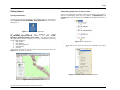
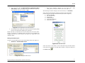
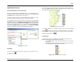
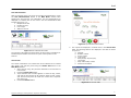
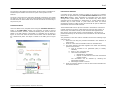
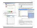
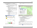
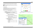
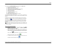
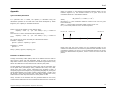
Rutgers Interactive Lane Closure
Application (RILCA) for
Work Zone Planning User Manual
Prepared for
Garden State Parkway
New Jersey Highway Authority
April 2007
Developed by:
Rutgers University Intelligent Transportation Systems Laboratory
Draft
Table of Contents
Introduction
Getting Started
Opening GIS Software
Adding Missing Shape Files to the Document
Setting Selectable Layers
Application Features
Zoom to Interchange / Zoom to Mile Post
Navigating
Link Selection
Link Characteristics
Volume Info
Toll Plaza Volumes
Lane Closure Schedule
Lane Closure Info
Incident Analysis
Appendix
Queue and Delay Estimation
Estimation of Mainline Volume
Rutgers Intelligent Transportation Systems Laboratory
Table of Illustrations
3
4
4
4
5
6
6
6
6
7
7
8
8
9
11
13
13
13
Figure
Figure
Figure
Figure
Figure
Figure
Figure
Figure
Figure
Figure
Figure
Figure
Figure
Figure
Figure
Figure
Figure
Figure
Figure
Figure
Figure
1 Shortcut to GIS Application
4
2 GIS application window
4
3 List of Shape files
4
4 Add data to replace missing shape files
4
5 List of shape files in the main directory
5
6 Setting Selectable Layers
5
7 GSP tool main menu
5
8 Zoom to MP
6
9 Zooming in the network
6
10 Select features icon in toolbar
6
11 Link characteristics table
7
12 Input Scenario Info window
7
13 Volume Info table
7
14 Toll Plaza Volume Info Window
8
15 Input Scenario Info window for lane closure schedule 9
16 Lane Closure Schedule Output
9
17 Lane Closure Schedule - Save File
9
18 Input Scenario Info for Lane Closure Info
10
19 Lane Closure Info table
10
20 Input Scenario Info for Incident Analysis
11
21 Incident Analysis table
11
2
Draft
Introduction
information and estimate the impact of lane closure scenarios at selected
locations.
An interactive computer tool for planning lane closures for work zones is
developed for the New Jersey Turnpike Authority (NJTA) Garden State
Parkway (GSP) division. This user-friendly tool is aimed at providing the
GSP engineers with a computerized and easy to use version of the Manual
for Traffic Control in Work Areas of the GSP along with various other useful
features.
This manual provides step-by-step information on how to use the GIS
decision tool.
The interactive software application is developed using ArcView GIS
software package as the main development environment. The interactive
GIS map of the GSP and its surrounding network is displayed using
ArcView and various analysis and visualization options are provided for
interactive planning of lane closures. The tool has the geometric details of
GSP and the surrounding highways and local streets. It provides users the
following applications:
Volume information on selected links at a given time period on any
given date.
Link characteristics (such as number of lanes, AADT, milepost, link
length).
A function that generates lane closure schedule for selected link based
on the 2005 and 2006 data processed by the Rutgers Intelligent
Transportation Systems (RITS) team.
A simple visualization function that shows the extent of expected
delays as a result of lane closure and possibility of spill back onto the
upstream links all in the form of link colors (delay estimations are
based on the Road User Cost Model developed by Urban Engineers,
Inc. for the NJTA).
Integrated lane closure cost estimation function (delay estimations are
based on the Road User Cost Model developed by Urban Engineers,
Inc. for the NJTA).
Delay estimation for incidents (based on the Road User Cost Model
developed by Urban Engineers, Inc. for the NJTA).
The volume information is generated using the monthly AADT information
gathered by the GSP and the electronic transaction dataset that was
provided by GSP. A new combined dataset was compiled by the RITS
Team. Hourly volumes on the mainline links are generated based on the
hourly volume factors obtained from the toll transaction data from the
nearest toll plaza. The details of the volume generation are presented in
the Appendix.
The developed tool provides the NJTA with a simple and interactive way to
navigate visually along the GSP corridor and gather link and volume
Rutgers Intelligent Transportation Systems Laboratory
3
Draft
Getting Started
Opening GIS Software
In order to open the GIS application, open (double-click) the shortcut icon
named Shortcut to NJ_STATEHWY_GSP_NJTPK.mxd on your desktop
(See Figure 1).
Adding Missing Shape Files to the Document
If any of the shape files are missing, follow the procedure shown below to
add the corresponding shape files. For instance, if Njnahighways and
counties shape files are missing in the Layers list will appear as shown in
Figure 3.
Figure 1 Shortcut to GIS Application
The
shortcut
is
linked
to
the
application
file
named
NJ_STATEHWY_GSP_NJTPK.mxd located in the folder C:\GSP
WorkZone Application\Shape Files Latest. This shortcut opens the
GIS application as shown in Figure 2. The map is composed of following
layers of GIS shape files:
1. GSP _Nodes
2. GSP_Mainline
3. GSP_AdjoiningStreets
4. Njnahighways
5. counties
These layers are listed on the left column of the GIS window under the
Layers menu as shown in Figure 2.
Figure 3 List of Shape files
1.
Right-click on the Layers list and select the Add Data (see Figure
4)
Figure 4 Add data to replace missing shape files
Figure 2 GIS application window
Rutgers Intelligent Transportation Systems Laboratory
4
Draft
2.
Then open the folder C:\GSP WorkZone Application\Shape
Files Latest, where the shape files are located (see Figure 5).
The shape files have the extension *.shp.
2.
Check the checkbox adjacent to the layer with
“GSP_Mainline” and press “Close” button (see Figure 6).
name
After finishing the above changes, save the document, i.e. File>Save.
In the document the following options are present in the Main Menu
present along the left edge of the document (as shown in Figure 7):
1. Zoom to Mile Post
2. Link Characteristics
3. Volume Info
4. Incident Analysis
5. Lane Closure Schedule
6. Lane Closure Info
Figure 5 List of shape files in the main directory
3.
In this folder all the shape files are present and the missing shape
files can be selected and added to the document.
Please note that it is imperative to have the shape files in the same order.
If they are present in a different order, the order can be adjusted by
dragging (with the left mouse button held down) the shape file to the
respective place.
Setting Selectable Layers
In order to set selectable layers in the main toolbar choose (see Figure 6).
1. Selection > Set Selectable Layers
Figure 7 GSP tool main menu
If the main menu is not visible, it can be activated using the RILCA button
in the Menu bar located in the GSP main window or using the shortcut in
the Tools toolbar
.
Figure 6 Setting Selectable Layers
Rutgers Intelligent Transportation Systems Laboratory
5
Draft
Application Features
In order to zoom in a desired location in the network, select the “Zoom In”
tool in the Tools toolbar and create a rectangle using the cursor around
the target location in the map (See Figure 9).
Zoom to Interchange / Zoom to Mile Post
The window corresponding to the Zoom option is open automatically as the
GIS tool is opened. If this window is not visible, it can be activated using
the Zoom button on the main menu (See Figure 7).
There are two ways to zoom in a desired location in the network. The users
can either select an interchange or type in the milepost number.
The interchange to which the user intends to zoom to can be selected from
the dropdown menu of interchanges in the northbound and southbound
directions present in the “Zoom to Interchange” section, and the zoom
button is to be pressed. Alternatively, the milepost of the link that has to
be selected should be entered in the textbox in the “Zoom to Milepost”
section and the Zoom button is to be pressed. The link with the milepost
entered is zoomed to in the map and selected and highlighted.
Figure 9 Zooming in the network
In order to navigate in the network, select the “Pan” tool in the Tools
toolbar
and drag the window in the desired direction. “Go Back to
Previous Extent” and “Go to Next Extent” tools can be use to select undo or
redo the zooming actions.
Link Selection
For all the other options in the Main Menu a link has to be selected. The
following procedure is to be followed to select a link:
1. In the Tools toolbar, choose the “Select Features” tool, as shown
in Figure 10.
2. Select the appropriate link using the mouse by clicking on the link.
The selected link is highlighted after selection.
Figure 8 Zoom to MP
Navigating
The entire network can be viewed by clicking on the “Full Extent” icon in
the Tools toolbar
Figure 10 Select features icon in toolbar
Rutgers Intelligent Transportation Systems Laboratory
6
Draft
Link Characteristics
After the selection of the link (using the procedure described above), press
the Link Characteristics button in the Main Menu window. After
selecting the time and the year information, the link characteristics are
displayed in a tabular form on the screen. The link characteristics table
includes (See Figure 11):
1. Milepost of the link
2. Number of lanes
3. Link Length
4. AADT for the link
Figure 12 Input Scenario Info window
5.
Figure 11 Link characteristics table
The columns of the table show the direction of each section (northbound or
southbound) and whether the section is a part of the express or local
sections.
Volume Info
The volume information of a selected link can be obtained for a selected
day, month, year and time period using the Volume Info button in the
Main Menu window.
1. Select the link using the procedure described in the Selection of
Links section.
2. Press the Volume Info button.
3. “Input Scenario Info” window appears in which the day, month,
year and the time period can be selected. Select the day, month,
year and the time period for which the volume info is required.
(See Figure 12)
4. Press the Continue button
The outputs are displayed in a tabular form in the Volume Info
table. The following features are displayed in the table as shown
in Figure 13:
a. Milepost
b. Number of lanes
c. Hourly volume
d. Time period
e.
Date (month, day and year)
f.
Link length
g.
Daily and monthly volume
h. Historical information
Figure 13 Volume Info table
Rutgers Intelligent Transportation Systems Laboratory
7
Draft
The columns of the table show the direction of each section (northbound or
southbound) and whether the section is a part of the express or local
sections.
The hourly volume and time period are displayed consecutively one beside
the other for each hour in the time period selected. The historical volume
info tab shows the same details of the volume info tab for the same day in
the previous year.
Toll Plaza Volumes
Users can obtain hourly toll plaza counts using the Toll Plaza Volume Info
button in the Main Menu window. The procedure is similar to that of
Volume Info button; however, instead of selecting a link, the list of the toll
plazas in the GSP network is presented in a dropdown box as shown in
Figure 14. Users can select the start and end hours and the desired date
for a selected toll plaza. The output is similar to the table given in Figure
13.
Lane Closure Schedule
A schedule for the minimum number of lanes to be open on a roadway
section can be generated using the Lane Closure Schedule button in the
Main Menu window. These schedules are generated using the Annual
Average Daily Traffic (AADT) data for the selected day. Lane closure
schedules can be generated for a selected day or a week starting with a
selected day for each month in years 2005 and 2006. An annual
percentage increase in traffic can also be entered as an input to obtain the
schedules for the future traffic demand.
The threshold traffic volume per lane involved in the decision of minimum
number of lanes to be open is 1350 vehicle per hour per lane (vphpl). In
other words, if the traffic volume per lane exceeds 1350 vphpl due to a
lane closure, then the lane closure is not warranted for. This process is
performed iteratively for all the lanes of the selected link over the selected
time horizon.
The generation of the Lane Closure schedules involves the following steps
(see Figure 15):
1. Select the link using the procedure described in the Selection of
Links section
2. Press the “Lane Closure Schedule” button on the Main Menu
3. The Input Scenario Info Menu appears from which the following
options can be chosen
a. Type of schedule to be generated (Daily or Weekly
schedule)
b. Date i.e. day, month and year
c. Lane closure information:
i. Northbound or southbound
ii. Express or local sections in the case of dual-dual
roadway section
The information can be selected by checking the
appropriate checkbox.
d. Percentage increase in volume
4. Press the Continue button to view the Lane Closure Schedule for
the selected scenario.
Figure 14 Toll Plaza Volume Info Window
Rutgers Intelligent Transportation Systems Laboratory
8
Draft
The columns of the table show the direction of each section (northbound or
southbound) and whether the section is a part of the express or local
sections. The schedule generated can be saved as an MS Excel document
(see Figure 17) using the “Save File” button on the Lane Closure Schedule
display form
File” button
. The same can be printed without saving using the “Print
.
The default folder or directory for the lane closure schedules is the C:\GSP
WorkZone Application\Shape Files Latest\Output directory within the
main directory C:\GSP WorkZone Application\Shape Files Latest.
Figure 15 Input Scenario Info window for lane closure schedule
In the Lane Closure Schedule is displayed in a tabular form as shown in
Figure 16. The table includes the following information:
1. Date
2. Day of the week
3. Hour
4.
Minimum number of lanes to be open for each hour on each day
Figure 17 Lane Closure Schedule - Save File
Lane Closure Info
The Lane Closure Info option can be used to generate the delays and
queues resulting from a particular lane closure scenario. The estimation of
delay and queue due to lane closure is based on the Road User Cost Model
developed by Urban Engineers, Inc. for the NJTA. The estimation functions
are presented in the Appendix.
Figure 16 Lane Closure Schedule Output
Rutgers Intelligent Transportation Systems Laboratory
The steps involved in the Lane Closure Info option are (see Figure 18):
1. Select the link using the procedure described in the Selection of
Links section
9
Draft
2.
3.
Press the Lane Closure Info button on the Main Menu window
The Input Scenario Info window appears from which:
a. The following options can be chosen from Time/Date
Info tab
i. Start and End hours for the lane closure scenario
ii. Date i.e. day, month and year
b. Lane closure information can be entered in the Lane
Closure Info tab:
i. Northbound or southbound
ii. Express or local sections in the case of dual-dual
roadway section. The information can be
selected by checking the appropriate checkbox
iii. Configuration of Lane Closure: “Exterior”, if the
lane is adjacent to median or curb and “Middle”
if otherwise.
c. Percentage increase in volume
d. The following parameters can be changed by the user in
the Other Parameters tab:
i. Lane Width of the roadway
ii. Average length of the vehicle (for queue length
calculations)
iii. Average gap between vehicles in queuing
conditions
iv. Capacity per lane under Normal and Work Zone
conditions
4. Press the Continue button to view the output for the selected
scenario.
Figure 19 Lane Closure Info table
The output of the Lane Closure Info option involves (see Figure 19):
1. Mile post of the selected link
2. Number of lanes on the selected link
3. Hourly volume for each hour in the selected scenario
4. Selected time period and date of the scenario
5. Number of closed lanes
6. Hourly Queue (vehicles)
7. Average Hourly Delay (hr/vehicle)
8. Total Hourly Delay (hrs)
9. Queue Length (miles)
The columns of the table show the direction of each section (northbound or
southbound) and whether the section is a part of the express or local
sections.
Figure 18 Input Scenario Info for Lane Closure Info
In addition to the above outputs, the maximum spill over of the queue is
highlighted on the map. In order to clear the highlighting from the display,
the refresh button
Rutgers Intelligent Transportation Systems Laboratory
must to be used. The case of any spill over of the
10
Draft
queue from the time period of the work zone operation is also considered.
The corresponding delays and queue lengths for the other hours are also
displayed.
Note: If the volume data for the time period chosen is not available, then
the volume of the most representative (same day from the previous year)
is chosen for analysis.
Incident Analysis
The Incident Analysis option can be used to generate the delays and
queues resulting from a particular occurrence of an incident. The
estimation of delay and queue due to lane closure is based on the Road
User Cost Model developed by Urban Engineers, Inc. for the NJTA. The
estimation functions are presented in the Appendix.
The steps involved in the Incident Analysis option are (see Figure 20):
1. Select the link using the procedure described in the Selection of
Links section
2. Press the Incident Analysis button on the Main Menu window
3. The Input Scenario Info window appears from which:
a. The following options can be chosen from Time/Date
Info tab
i. Start hour of the incident scenario
ii. Date i.e. day, month and year
iii. Duration of the incident in minutes.
b. Lane information can be entered in the Incident Info
tab:
i. Northbound or southbound
ii. Express or local sections in the case of dual-dual
roadway section. The information can be
selected by checking the appropriate checkbox
c. Percentage increase in volume
d. The following parameters can be changed by the user in
the Other Parameters tab:
i. Lane Width of the roadway
ii. Average length of the vehicle (for queue length
calculations)
iii. Average gap between vehicles in queuing
conditions
iv. Capacity per lane under Normal and Incident
conditions
Figure 20 Input Scenario Info for Incident Analysis
4. Press the Continue button to view the output for the selected
scenario.
Figure 21 Incident Analysis table
Rutgers Intelligent Transportation Systems Laboratory
11
Draft
The output of the Incident Analysis option involves (see Figure 21):
1. Start time and duration of the incident
2. Mile post of the selected link
3. Number of lanes on the selected link
4. Hourly volume for each hour in the selected scenario
5. Selected time period and date of the scenario
6. Number of closed lanes
7. Hourly Queue (vehicles)
8. Average Hourly Delay (hr/vehicle)
9. Total Hourly Delay (hrs)
10. Queue Length at the end of each hour (miles)
11. Maximum queue length (miles)
The columns of the table show the direction of each section (northbound or
southbound) and whether the section is a part of the express or local
sections.
In addition to the above outputs, the maximum spill over of the queue is
highlighted on the map. In order to clear the highlighting from the display,
the refresh button
must to be used. The case of any spill over of the
queue from the time period of the work zone operation is also considered.
The corresponding delays and queue lengths for the other hours are also
displayed.
Note: If the volume data for the time period chosen is not available, then
the volume of the most representative (same day from the previous year)
is chosen for analysis.
Notes on Saving and Printing output:
1. Users are advised to save their output files in the Output
subfolder
in
the
main
directory
C:\GSP
WorkZone
Application\Shape Files Latest.
2.
Users are advised to save their output files using different file
names when creating lane closure schedule at the same link for
various scenarios. The output generated can be saved using the
“Save” button
3.
. Alternatively, the output can be printed
without saving using the “Print” button
.
An additional utility provided is the calculator function that can be
accessed using the calculator button
.
Rutgers Intelligent Transportation Systems Laboratory
12
Draft
Appendix
plaza. For instance, in the following hypothetical mainline sketch, for the
mainline segment 3-4, the mainline volume for a given hour on the
northbound direction is calculated as follows:
Queue and Delay Estimation
If a particular lane is closed, the capacity is calculated using the
calculations specified in the Road User Cost Model developed by Urban
Engineers, Inc. Capacity is calculated as follows:
If lane is next to the median or curb (Exterior lane),
Capacity = 1600 * (1 - (12 - lane width) * (0.1)) * number of
lanes
If the lane is in a more centralized location (Middle lane),
Capacity = 1500 * (1 - (12 - lane width) * (0.1)) * number of
lanes
For a given hour the queue and delay are calculated as follows:
If Volume > Capacity
Queue = (Volume – Capacity) + Queue
If Capacity > Volume
Queue = 0
Delay = (Delay+ (Queue / Capacity))*0.5
NB_Volumei (3-4) = AADT (3-4) * HFi (1)
Where,
NB_Volumei (3-4) is the northbound mainline volume on link 3-4 at a given
hour indexed by i.
AADT (3-4) is the average annual daily traffic volume on link 3-4.
HFi (1) is the hourly factor for hour i for the toll plaza 1.
Toll Plaza - NB
1
Toll Plaza - SB
2
Toll Plaza- SB
3
4
5
Please note that the hourly factors for the northbound traffic on the
mainline are obtained from the closest toll plaza that has tollbooths on the
northbound. Similarly, for link 3-4 on the southbound direction, the hourly
factors are obtained from toll plaza 5, since it is closer to link 3-4 than toll
plaza 2.
Estimation of Mainline Volume
Average annual daily traffic (AADT) data set is obtained from the GSP for
each month in 2005 and until September 2006. In order to convert the
daily traffic volume to hourly volumes for the mainline segments the hourly
factors are obtained from the electronic toll collection (ETC) data.
The ETC dataset includes vehicle-by-vehicle entry and exit time data, such
as toll plaza index (interchange index), tollbooth lane index, time, date,
vehicle type (cars, trucks, buses), transaction type (E-ZPass or cash). A
computer program is developed in C programming language for parsing the
vehicle-based dataset (one month of data is approximately 1.5 GB in text
file format). Using this computer code, RITS team calculated the hourly
traffic factors for each day and month for all toll plazas on GSP.
Hourly volumes on the mainline links are generated based on the hourly
volume factors obtained from the toll transaction data from the nearest toll
Rutgers Intelligent Transportation Systems Laboratory
13