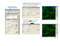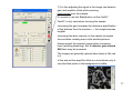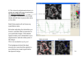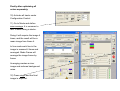
Download 100305 Zeiss guide

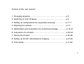
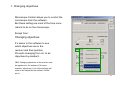
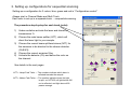
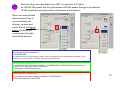
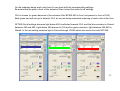
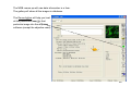
Zeiss LSM 510 META
user manual
Hege Avsnes Dale, Molecular Imaging Center, UiB
1
Open the LSM
software in expert
mode
The software opens
like this:
2
OBS! Before looking at the sample in the microscope press the VIS button.
For regular imaging you need the 4 first windows in the acquire menu (marked red).
3
Content of this user manual:
1. Changing objective…………………………………………………p 5
2. Switching on and off lasers………………………………………..p 6
3. Setting up configurations for sequential scanning………….…..p 7-11
4. Adjusting the pinhole……………………………………………….p 12
5. Optimization and acquisition of a multicolored image….……….p 13-21
6. Acquisition of a Z-stack…………………………………………….p 22-24
7. Saving the images………………………………………………….p 25-26
8. Setting up for DIC (transmission) imaging……………………….p 27-30
9. Time series………………………………………………………….p 31-32
4
1. Changing objectives
Microscope Control allows you to control the
microscope from the software.
But these setting are most of the time more
natural to do on the microscope.
Except from:
Changing objectives
It’s easier in the software to see
which objectives are in the
revolver and their position.
Prevents changing from oil- to airobjectives by accident…
OBS: Changing objectives in the revolver must
be registered in the software (File menu;
maintain; objectives), if not all the settings will
relate to the objectives the software “thinks”
are in.
5
2. Switching on and off lasers
Switch only on the lasers you need!
If lasers are on when you start, switch off
the ones you’re not using.
The lasers have different power ranging
from 1 to 30 mW.
The Argon laser is the strongest laser and
has its own output (%) slider in the laser
control window. It is turned on in standby.
When status comes up as ready it can be
switched on. Never work in standby and
always use 40 % output as a starting point.
Turning on this laser automatically starts a
fan. When turning off the fan automatically
stops after a while and until it stops the
remote control must not be switched off!
All other lasers are only switched on and off
and has no fan.
6
IN GENERAL: 405 nm excites blue (DAPI), 488 nm excites green, 543 nm excites red and 633 nm excites far red.
3. Setting up configurations for sequential scanning
Setting up a configuration for 3 colors, blue, green and red in “Configuration control”.
Always start in Channel Mode and Multi Track.
Each color is set up in a separate track → sequential scanning.
The procedure step by step for each track (color):
1)
2)
3)
4)
5)
Under excitation activate the laser and choose a
transmission %.
Choose the main beam splitter (HFT), which will
direct the laser light to your sample.
Choose the correct beam splitters/mirrors (NFT) for
the emission to be directed to the chosen detector
(ChS/2/3).
Choose the correct emission filter.
Activate the detector (Ch) and define the color on
the channel.
See details in the next pages.
3
3
2
HFT = Haupt Farb Tailer → The numbers indicate which laser is
reflected towards the sample.
NFT = Neben Farb Tailer → The number indicate where the light
is split, ex. NFT490; all light below 490
nm is reflected, and light above 490
passes through.
4
5
1
7
1
Activate laser (only one
for each track).
Remember to turn on
laser in Laser Control.
Choose transmission %.
Typical values for:
405 nm: 5%
488 nm: 5%
543 nm: 80%
633 nm: 50%
(These values can be
changed later during image
optimization.)
2
Choose the main beam
splitter (HFT).
This reflects laser light to
the sample, whereas the
emission light will pass
through on its way back.
The wavelength of the
laser light needs to be
represented in the beam
splitter.
Ex: Using 405 laser →
405 needs to be present.
A TIP:
If you want to set up more
than one track (color),
pick the HFT that also
reflects the lasers you
plan to use in the next
tracks.
8
3
Choose the beam splitters to direct the emission light to the correct emission filter and detector.
At this point you need to know where to detect the signal.
This is decided based on the emission filters in front of the detector.
For regular imaging Ch2 and Ch3 are the most frequently used.
In general Ch2 can be used for blue and green, Ch3 can be used for green, red, and far red (see
next page).
If all the light can
go towards Ch2
& 3 use a mirror.
The NFT can also be
picked to fit all planned
tracks (colors).
In this case blue
emission needs to be
directed towards Ch2.
All NFTs incl. the mirror
would be ok for this.
But planning ahead NFT
490 is best suited (more
page 10).
NFT 490 means that all
light below 490 nm is
reflected up, everything
above 490 passes
through.
9
4
Emission filters are either Band Pass (BP) or Long Pass (LP) filters.
Ex. BP420-480 means that the light between 420-480 passes through to the detector.
LP420 means that everything above 420 passes to the detector.
When you have decided
which emission filter to
use and thereby the
detector, go back and
check that the 2nd beam
splitter will direct the
correct part of the light
towards the detector.
Setting up for blue emission:
Use BP420-480.
(If LP420 is chosen you risk including emission from any autofluorescence excited with the 405 laser, or any
emission from cross excitation of another stain present in the sample.)
Setting up for green emission:
If you plan to use a red stain in addition : Use BP505-530 or BP505-550 (preferably the last; to
include as much of the green emission as possible).
If only green: LP505 may be used.
Setting up for red emission:
If you plan to use a far red stain in addition: Use BP560-615
If red is the last color: Use LP560.
10
On the schemes below each color has it’s own track with the corresponding settings.
Be aware that the path in front of the emission filters is kept the same for all settings.
Ch3 is chosen for green because of the emission filter BP505-550 in front (not present in front of Ch2).
Both green and red can go to detector Ch3, as we are doing sequential scanning of each color at the time.
NFT490 fits all settings because light below 490 is reflected towards Ch2, and the blue emission is filtered
between 420 and 480. Light above 490 passes to Ch3 and for green emission, light between 505-550 is
filtered. In the red setting emission light is filtered through LP560 which also works fine with NFT490.
11
4. Adjusting the pinhole
Go to the Scan control window in Channels.
Define airy unit 1 for the green channel and copy the pinhole diameter into the blue and red channel.
The airy unit will now slightly differ between the different colors, but the thickness of the optical slice will
theoretically be the same.
Optical slices thickness
with airy unit at 1 for all
pinholes → thickness vary
between colors.
Optical slices thickness
with the same diameter for all
pinholes → thickness
between colors is the same.
The green channel is chosen as a
reference because it’s the channel in the
middle and will represent a mean value
for the pinhole diameter.
OBS!
If you change the objective
pinholes must be adjusted again.
12
5. Optimization and acquisition of a multicolored image.
For optimizing the image you work between Channels and Mode in the Scan Control window.
Optimization has to be done for each Channel (color).
13
The optimization procedure step by step:
(see more details in the following pages)
1)
Activate only one channel at the time in Configuration Control. Start with the color that frames
what your interested in in the sample.
2) Go to Scan Control Mode. Make a starting image with low zoom (detector gain for the first
image can be found with the button Find).
3) Define the zoom. Use the Crop button on the side of the image. If you want to be consequent
and use the same zoom between images type in the zoom factor.
4) Optimize the frame size. This will give the correct numbers of pixels for acquiring the image
with optimal resolution (dependent of chosen zoom and the objective used).
5) Adjust the scan speed by setting the pixel time to a value between 1,5 and 2,5 µsec.
6) Put on the range indicator, which is found under the button Palette on the side of the image.
Saturated pixels appear red and pixels below zero are blue.
7) Go to Channels and fine adjust the signal in the image by adjusting Detector gain and/or Laser
intensity then Amplifier offset while scanning continuously over the sample. Never use the
FastXY-button, always the Cont button. Increasing gain and laser intensity increases the
signal, but first adjust the gain and when this is around 800, the laser should be increased
instead. Increasing amplifier offset decreases blue pixels in the image.
8) Adjust to avoid red and blue pixels in the image.
9) Do the same with the next Channels (colors), point 2-5 will be remembered by the software so
you only have to do adjustments in the Channel window.
10) With all channels optimized, activate them all in the Configuration Control.
11) Go to mode and define averaging, 4 is common to use (in Z-stacks 2).
12) Press the single button and the final images are acquired.
14
1)
Activate only one
Channel at the time.
2) Begin with a starting image with low
zoom, 0.7 will give you the largest
possible image on the screen.
3) Define the crop. If you want to
always keep the same zoom
factor, it can be typed in.
15
4) After defining the zoom press Optimal under
Frame Size. This will define how many pixels
you need for optimal resolution for the chosen
zoom (and objective).
Be aware that the optimal resolution for different
colors will vary. So always optimize with the
same color in different images.
When combining the colors blue, green and red,
green will again give the mean value and should
be used when optimizing.
5) Adjust the scan speed. The pixels time should
be somewhere between 1,5 and 2,5 µsec. Going
too slow will take too much time and might
bleach the sample. Going too fast will not give a
nice signal.
6) Put on range indicator
found under the Palette
on the side of the image.
16
7) For fine adjusting the signal in the image use detector
gain and amplifier offset while scanning
continuously over the sample.
It’s crucial to use the Cont button not the FastXY.
FastXY is only used when focusing the sample.
Increasing the gain increases the detectors amplification
of the photons from the emission → the image becomes
brighter.
Increasing the laser intensity on the sample increases
the excitation creating more initial emitted photons.
Always exploit the detector range before increasing
laser (avoiding bleaching). But at detector gain around
800 laser may be increased.
The images are generally optimal when there is little red
in it.
In the end set the amplifier offset to a level where only a
very few blue pixels in the background is visible.
17
8) The intensity adjustments done is to
create an image with grey levels within
the dynamic range of 256
(8 bit image). Each pixel in the image
ideally should have a grey scale value
of 0 to 256.
Red & blue pixels will not have any
quantitative value.
But when adjusting the intensities you
have to consider what is important in
your particular image. If the weaker
signal is what you’re interested in you
might need to saturate other parts of
the image.
This is an evaluation up to you!
The background should be kept
around zero (very few blue pixels) to
avoid hiding any weak signal below
the dynamic range.
Highly saturated
No saturation
18
9) Do similar adjustments
on the following channels
(colors).
Everything in the Mode
window is remembered by
the software (zoom, frame
size, scan speed).
You only have to optimize
the intensities in the
image.
19
Finally after optimizing all
colors separately:
10) Activate all tracks under
Configuration Control.
11) Go to Mode and define
scan average. 4 is common to
use. 2 when doing z-stacks.
Doing 4 will acquire the image 4
times, and the result will be a
mean image from those 4.
In line mode each line in the
image is scanned 4 times and
averaged. Mode Frame will
average the image frame by
frame.
Averaging creates a nicer
image and reduces background
noise.
12) Press single and the final
image is acquired.
20
The range indicator can now be changed to no
palette and the different colored images are created
sequentially. The result is 3 single images and one
overlay in the same file.
At the bottom of the image the total and remaining
acquisition time comes up.
21
6. Acquisition of a Z-stack.
Z-stack step by step:
(more details next pages)
1)
2)
3)
4)
5)
6)
7)
Always start by optimizing each color separately like shown in chapter 5. But be aware:
Optimize each color in the brightest optical slice (focal plane). This might not be the
same plane for all colors. For each color focus with FastXY through the stack and stop
at the brightest focal plane and optimize.
Activate only one color when defining the stack. Use the one that frames what you’re
interested in.
Activate Z-stack in Scan Control and chose Mark First/Last.
Define the borders of the Z-stack. Scan FastXY and focus to one end of the stack and
Mark First, then go back into the sample to the next border and Mark Last.
Go to Z Slice and click Optimal Interval to define the total number of optical slices
through the stack.
Go to Mode and define averaging to 2 (optional).
Start the scan. The time it takes will come up under the image.
22
1)
2)
3)
4)
5)
6)
7)
Optimize the different
colors.
Activate the man channel
(color) of interest.
Activate Z stack.
Choose Mark First/Last.
Focus with FastXY to one
border of the sample, stop
when the fluorescence is
getting dim and Mark First.
Then go back through the
sample and decide on the
other border Mark Last.
Total Z-stack depth comes
up.
Click on Z Slice and
choose Optimal Interval.
The optical slices will the
overlap 50%.
23
NB! You do not have to optimize the interval, this will only ensure the best resolution for a potential 3D
reconstruction. You may define fewer slices just to get an overview in different focal planes in the sample.
Remaining and total Z-stack acquiring time.
The progression of the Z-stack may be viewed in Gallery, and if you see that the images
contains no more information, the scan can be stopped any time.
24
7. Saving the images
1)
2)
3)
4)
5)
6)
Press Save as on the image.
When saving the first time you have to define the
database (MDB) where the images should be saved.
A database per date you work may be a way to
organize the databases. Choose New MDB and
define where to save it. We encourage all to save on
our external server Biomic on ‘skule’. (For this you
need access to the server, for more info contact MIC
personnel or Torstein Ravnskog.) You may also open
an existing MDB.
Then enter the name of the image.
The next image to be saved will automatically be
saved in the previous defined database (coming up in
blue).
All images will have the file format .lsm and can only
be read in LSM software or processing software that
reads lsm-files (like Imaris, ImageJ etc.). A free Zeiss
LSM browser can be download; go to the MIC
webpage, then to Equipment and Zeiss LSM 510
META. At the bottom of the page you’ll find the link.
You can export images to all common file formats, but
never delete the raw data files!
25
The MDB comes up with raw data information in a form.
The gallery will show all the images in database.
The Reuse button will help you load
all the parameters used for that
particular image into the acquiring
software (except the objective used).
26
8. Setting up for DIC (transmission) imaging.
DIC (Differential Interference Imaging) step by step:
(more details on the next pages)
1)
2)
3)
4)
5)
6)
7)
8)
If you want to do a multicolored image with DIC do everything as described in chapter 3 and the
proceed with the following steps.
Adjust the Köhler Illumination on the microscope.
Choose the DIC filter in the condenser in the Microscope control window. For air objectives DICII,
for immersion objectives DICIII.
The DIC channel can be set up in any track in combination with any other emission Channel and
laser. Activate channel D (ChD) and inactivate the current Ch (detector) in the setup.
Press Find to find the detector gain.
Use FastXY to find the best focus for DIC.
Fine adjust the gain and offset to visually get the best DIC image.
Activate the other Channel in the current setup.
27
2) Adjusting the Köhler illumination – Essential for acquiring a nice DIC image!!
Polarizer D
The
condenser
in an
inverted
microscope
Condenser
focusing screws
Felt blender
Condenser
centering screws
1. Close the felt blender until
you se the polygon and focus
this with the vertical adjustments
screws. If the polygon is not
visible to begin with focus the
condenser until you see it.
2. Center the polygon
with the centering
screws.
3. Open the felt blender
like this and fine adjust
the centering.
4. Open the felt blender
until you see the full
view field.
28
3)
4)
5)
6)
7)
Choose a DIC filter in the
Condensor (for air objectives DICII,
for immersion objectives DICIII).
Activate the transmission detector
ChD and inactivate the current
emission channel (in the example
Ch2 for Blue emission).
Do a Find for getting a detector
gain.
Fine adjust focus with FastXY if
necessary.
Fine adjust detector gain and offset
if necessary.
29
8)
Finally activate the all the different tracks and channels (colors), choose averaging in Mode and
do a Single.
Notice that the DIC image is in this example in the track for blue. This means that the DIC image
comes up simultaneously with the blue image, and is created with the 405 nm laser.
The DIC image could in principle have been put in any of the tracks.
The DIC image comes as a separate image and in the overlay image in the lsm file.
A DIC image can be acquired alone and later copied into the colored images. But be aware that
copying will only work if the images to be copied together has exactly the same frame format.
30
9. Time series
Doing live cell imaging there are several considerations. Mainly one has to keep the cells happy during the
acquisition of the time series.
Before acquiring you need to warm up the heating chamber, ideally a couple of hours before imaging to
stabilize the system. Turn on the Temperature Control and the Heater.
When placing the cells under the microscope, make sure to use the right insert. If you need CO2 put on the
CO2-lid on top of the stage and switch on the CO2-controller (switch on the back of the control box). This is
previously set to give approx. 5 % CO2 at the sample.
It’s a good idea to let the cells acclimatize for some time and to watch the potential focus drift in the beginning
of a time lapse.
The settings has to be defined ahead of staring the time series more or less as described in chapter 3, but to
keep cells happy over time you most likely need to make a compromise on image quality and thereby not
necessarily use optimal frame size. Perhaps you also need to increase the pixel time below the recommended
1,5 µsec.
It’s is always a good idea to minimize laser intensity on the sample, and to be able to do that opening the
pinhole to let more light come to the detector is an option, but this will be a compromise on resolution in Z.
31
When you’re satisfied with the settings for acquisition open Time Series Control.
Define how many images
the time series will consist of
in Stop series, which means
stop series after the number
of scans chosen.
Choose the Cycle Delay, the
time between images
(singled or multi-colored) or
eventually Z-stacks.
You may follow the time series coming up in
the gallery. You can stop the scan any time.
Start the time series.
Follow the focus over some
time. If focus drifts stop the
scan, refocus and start the
time series over again.
32
Countdown until next image in the time series.