1
SISO-GPCIT
GENERALIZED PREDICTIVE CONTROL
INTERACTIVE TOOL FOR SISO SYSTEMS
Authors:
José Luis Guzmán
Manuel Berenguel
Sebastián Dormido
2
Referencia al internal report:
GPCIT - Generalized Predictive Control Interactive Tool1 .
c José Luis Guzmán∗ , Manuel Berenguel∗ , Sebastián Dormido∗∗
∗
Universidad de Almerı́a, Dpto. de Lenguajes y Computación, Área de Ingenierı́a de
Sistemas y Automática, Ctra. Sacramento s/n, 04120 Almerı́a, Spain. Tel. +34 950 015683,
Fax. +34 950 015129, E-mail: [joguzman,beren]@ual.es.
∗∗
Universidad Nacional de Educación a Distancia, Dpto. de Informática y Automática,
Avda. Senda del Rey n.7, 28040, Madrid, Spain. Tel. +34 91 ——-, Fax. +34 91 ——- ,
E-mail: [email protected]
1
submitted to IEEE Control Systems Magazine - 2003
Contents
1 Introduction
1
2 Sections of the tool
3
2.1
Graphics . . . . . . . . . . . . . . . . . . . . . . . . . . . . . . . . . . . . . . .
3
2.2
Parameters section . . . . . . . . . . . . . . . . . . . . . . . . . . . . . . . . .
10
2.3
Menus . . . . . . . . . . . . . . . . . . . . . . . . . . . . . . . . . . . . . . . .
16
3 Examples
19
3.1
Unconstrained case example . . . . . . . . . . . . . . . . . . . . . . . . . . . .
19
3.2
T-polynomial . . . . . . . . . . . . . . . . . . . . . . . . . . . . . . . . . . . .
20
3.3
Constraints . . . . . . . . . . . . . . . . . . . . . . . . . . . . . . . . . . . . .
21
3.3.1
Physical limitations and security contraints . . . . . . . . . . . . . . .
22
3.3.2
Performance constraints . . . . . . . . . . . . . . . . . . . . . . . . . .
23
3.3.3
Constraints and stability . . . . . . . . . . . . . . . . . . . . . . . . . .
26
3.3.4
Constraints combination . . . . . . . . . . . . . . . . . . . . . . . . . .
29
Stability issues . . . . . . . . . . . . . . . . . . . . . . . . . . . . . . . . . . .
30
3.4
i
ii
CONTENTS
List of Figures
2.1
Main view of the tool
. . . . . . . . . . . . . . . . . . . . . . . . . . . . . . .
4
2.2
Plant + Model. . . . . . . . . . . . . . . . . . . . . . . . . . . . . . . . . . . .
5
2.3
Example of modification of N2 . . . . . . . . . . . . . . . . . . . . . . . . . .
5
2.4
Example of set-point modification
. . . . . . . . . . . . . . . . . . . . . . . .
6
2.5
Example of including unmeasured disturbances . . . . . . . . . . . . . . . . .
6
2.6
Example of constraints acting on the output . . . . . . . . . . . . . . . . . . .
7
2.7
Control signal and control increment . . . . . . . . . . . . . . . . . . . . . . .
7
2.8
Modification of Nu in the control increment window . . . . . . . . . . . . . .
8
2.9
Constraints in input amplitude and input increment . . . . . . . . . . . . . .
8
2.10 Location of poles and zeros in the s and z planes . . . . . . . . . . . . . . . .
9
2.11 Modification of the length of the simulation . . . . . . . . . . . . . . . . . . .
9
2.12 Output scaling . . . . . . . . . . . . . . . . . . . . . . . . . . . . . . . . . . .
10
2.13 Scaling of poles and zeros . . . . . . . . . . . . . . . . . . . . . . . . . . . . .
10
2.14 Values in the task bar . . . . . . . . . . . . . . . . . . . . . . . . . . . . . . .
11
2.15 Parameters control . . . . . . . . . . . . . . . . . . . . . . . . . . . . . . . . .
11
2.16 Adding poles . . . . . . . . . . . . . . . . . . . . . . . . . . . . . . . . . . . .
12
2.17 Modification of the delay . . . . . . . . . . . . . . . . . . . . . . . . . . . . . .
12
2.18 Sliders over control parameters . . . . . . . . . . . . . . . . . . . . . . . . . .
13
iii
iv
LIST OF FIGURES
2.19 Modification of the number of set-point changes . . . . . . . . . . . . . . . . .
13
2.20 Example of output band constraints . . . . . . . . . . . . . . . . . . . . . . .
14
2.21 Example of final state constraint . . . . . . . . . . . . . . . . . . . . . . . . .
15
2.22 Example of clipping . . . . . . . . . . . . . . . . . . . . . . . . . . . . . . . .
15
2.23 Menu Settings . . . . . . . . . . . . . . . . . . . . . . . . . . . . . . . . . . . .
16
2.24 Visualizing the discretization methods . . . . . . . . . . . . . . . . . . . . . .
16
2.25 Dialog box to modify the transfer function . . . . . . . . . . . . . . . . . . . .
17
3.1
Simple Example. Initial Configuration. . . . . . . . . . . . . . . . . . . . . . .
19
3.2
Modification of control parameters . . . . . . . . . . . . . . . . . . . . . . . .
20
3.3
Disturbance rejection. T-Polynomial. . . . . . . . . . . . . . . . . . . . . . . .
21
3.4
Unstable plant. Output amplitude constraints . . . . . . . . . . . . . . . . . .
22
3.5
Unstable plant. Input constraints . . . . . . . . . . . . . . . . . . . . . . . . .
23
3.6
Nonminimum phase behavior constraint. . . . . . . . . . . . . . . . . . . . . .
24
3.7
Monotonous behavior constraint. . . . . . . . . . . . . . . . . . . . . . . . . .
25
3.8
Overshoot constraint. . . . . . . . . . . . . . . . . . . . . . . . . . . . . . . .
26
3.9
Output band constraint. . . . . . . . . . . . . . . . . . . . . . . . . . . . . . .
26
3.10 Unstable output. Without CRHPC. . . . . . . . . . . . . . . . . . . . . . . .
27
3.11 CRHPC activation. . . . . . . . . . . . . . . . . . . . . . . . . . . . . . . . . .
28
3.12 Modification of λ in CRHPC. . . . . . . . . . . . . . . . . . . . . . . . . . . .
28
3.13 Constraints combination . . . . . . . . . . . . . . . . . . . . . . . . . . . . . .
29
3.14 GP C∞ strategy. . . . . . . . . . . . . . . . . . . . . . . . . . . . . . . . . . . .
30
3.15 First stability theorem of Zhang . . . . . . . . . . . . . . . . . . . . . . . . . .
32
3.16 Second stability theorem of Zhang . . . . . . . . . . . . . . . . . . . . . . . .
33
List of Tables
2.1
Constraints included in the tool and checkbox correspondences. . . . . . . . .
v
14
vi
LIST OF TABLES
Chapter 1
Introduction
SISO-GPCIT (Single Input Single Output Generalized Predictive Control Interactive Tool )
is an interactive tool for control education developed with Sysquake ([7]). Its objective
is to help the students to learn and understand the basic concepts involved in Generalized
Predictive Control (GPC)[2],[3]. Using this tool the student can put into practice the adquired
knowledge on this control technique using simple examples of unconstrained cases, effect of
plant/model mismatch and robustness issues, disturbance rejection, effect of constraints in
the design and performance of the controller, stability issues, etc. Thus, using this tool the
student can better understand the underlying theory interactively. It is possible to analyse
how the closed loop system response is affected by changes in different design parameters
such as weighting factors δ (on tracking errors) and λ (on control effort), the prediction (N1
and N2 ) and control (Nu ) horaizons, the sample time, the T-polynomial, etc. At the same
time, different constraints related to physical limits or security issues, desired performance or
stability can be selected and activated to see their effect on the performance of the controlled
system.
This document is a tutorial of the tool. The second chapter presents a description of
its main parts and how to use it. Once the user is familiarized with it, the third chapter
introduces a set of examples (with increasing complexity) which objective is to facilitate the
student see some interesting features of GPC. All these examples are available in the tool.
1
2
CHAPTER 1. INTRODUCTION
Chapter 2
Sections of the tool
Three types of elements can be distinguished in the tool: graphics, section of parameters and
menus. The first one is composed by the different graphs that show the output and input
to the system, disturbances, set-points and poles and zeros locations for both the model and
the plant and in the s and z planes. On these graphs it is possible to interactively modify a
lot of parameters: control and prediction horizons, graphs scaling, poles and zeros location,
constraints, etc. The second set of elements allows modifying the control and simulation
parameters, those corresponding to the plant and model transfer functions, as far as those
constraints imposed to the system (and other options). The third set of elements is linked to
the menu Settings, from which it is possible to modify the discretization method for the plant
and model transfer functions, the value of the sample time, the T-polynomial, the values of
the transfer function coefficients of the plant and the model, select automatic or manual
scaling of figures, accessing this tutorial and load different illustrative examples. A general
view of the tool can be seen in figure 2.1. In what follows, the different elements of the tool
are described.
2.1
Graphics
In this part of the tool several graphs containing the output of the system, the control signal
and control increments, the plant and model poles and zeros locations, both in s and z planes
are shown.
The figure located at the lower left part of the screen 2.1 shows the output of the system
with the name Constraints y. Several elements differentiated in shape and color are shown:
• Both the output of the real plant (in green color) and that of the model (in orange
color) are displayed. This distinction allows analysing the system response in the face
of modeling errors (see figure 2.2).
3
4
CHAPTER 2. SECTIONS OF THE TOOL
Figure 2.1: Main view of the tool
2.1. GRAPHICS
5
Figure 2.2: Plant + Model.
• Two dotted blue vertical lines represent the prediction horizons N1 and N2 . To modify
the value of each of them it is only required to place the mouse pointer over them and
drag them to the left or to the righ, to decrease or increase their values. An example in
which the upper prediction horizon is modified is shown in figure 2.3, where it can be
seen how the system response changes when N2 is modified from 4 to 8 sample times.
(a) Value of N2 = 4
(b) Value of N2 = 8
Figure 2.3: Example of modification of N2
• Another element is the set-point, represented as a step using violet color. A small circle
of the same color is placed over this curve in the place corresponding to the sample
time in which the step is produced. Using this circle it is possible to modify both
the amplitude and the time instant in which the step is introduced, in the same way
explained with the prediction horizons, that is, using the mouse pointer and dragging
it vertically (amplitude modification) or horizontally (modification of the step time).
Figure 2.4 shows an example of set-point modification.
• Over the y = 0 line a set of small circles can be observed, used to generate unmeasured
disturbances in the form of step (black circles), impulse (red circles) and noise (green
circles). By modifying their vertical position the amplitude of the selected disturbance
can be changed, and modifying their horizontal position the instant from which the
disturbance acts on the output of the system can be changed. The activation of the step
and impulse disturbances is immediate. To incorporate the noise disturbance, a checkbox
6
CHAPTER 2. SECTIONS OF THE TOOL
(a) Amplitude = 0.8 Instant = 0
(b) Amplitude = 1.288 Instant = 11
Figure 2.4: Example of set-point modification
has to be activated in the parameters control block, as will be commented in the next
section. An example of step disturbances in sample times 13 and 24 with amplitudes
0.293 and 0.007 respectively is shown in figure 2.5. In the instant 29 an impulse of
amplitude 0.493 is also introduced and finally a noise disturbance of amplitude 0.1943
is activated in the 35 sample time. The composition of all these signals is shown as a
black dotted line.
(a) Without disturbances
(b) With disturbances
Figure 2.5: Example of including unmeasured disturbances
• The rest of modifiable elements are the following constraints: output amplitude constraints, final state constraints and band constraints. When those constraints are activated in the corresponding checkboxes (see section 2.2) their values are represented
using horizontal, vertical and exponential lines respectively, being possible to modify
their values/positions by dragging them vertically (output amplitude and band) or horizontally (final state). The modification of the band constraint is carried out using the
circles that appear at the end of those curves, while the rest can be moved by selecting
and dragging any point of the lines, as was previously commented in the case of prediction horizons. The output amplitude constraints are represented by two red horizontal
lines (figure 2.6 (a)), those of the final state with two cyan vertical lines (figure 2.6 (b))
and those of band type with two curves of the same colour with an exponential shape
2.1. GRAPHICS
7
(first order system step response) (figure 2.6 c).
(a) Output amplitude constraint
(b) Final state constraint
(c) Output band constraint
Figure 2.6: Example of constraints acting on the output
The other graphics that are included in the tool allow the visualization of the control
signal and its increment (resulting from the minimization of the GPC cost function). Such
graphs are those appearing in figure 2.1 named Constraints in U and Constraints in DU
respectively. The different elements shown in these graphs are:
• The input of the system (control signal) is represented in ligth green color, while the
control increment is represented in brown color, as it is shown in figures 2.7 (a) and 2.7
(b) respectively.
(a) Control signal U
(b) Control signal increment DU
Figure 2.7: Control signal and control increment
• In both figures a vertical magenta line represents the control horizon. To modify its
value it is only necessary to place and drag the mouse pointer over this line, being
possible to increase or decrease its value. An example of a change from 3 to 9 sample
times is shown in figure 2.8.
• When the constraints in the input amplitude and increment signals are activated (or the
clipping option), their maximum and minimum values are represented by two horizontal
8
CHAPTER 2. SECTIONS OF THE TOOL
(a) Nu = 3
(b) Nu = 9
Figure 2.8: Modification of Nu in the control increment window
lines in both graphics, in the same way the output amplitude constraint is represented
in the Constraints in Y graph. In this way, by modifying the position of these horizontal lines, the value of the associated constraint is changed. Those constraints can
be appreciated in figure 2.9.
(a) U constraint
(b) DU constraint
Figure 2.9: Constraints in input amplitude and input increment
Two more graphics are shown in the tool: those corresponding to the location of poles
and zeros both in the s and z planes (figure 2.10), as far as the T-polynomial roots and
the closed-loop system poles. These graphics have the name continuous-time poles and zeros
and discrete-time poles and zeros. The poles are represented using the × symbol and the
zeros using ◦. The poles and zeros of the plant are of green-blue color and those of the
model in orange color, using the same color convention that for the dynamical evolution of
the plant/model in figure 2.2. The closed-loop system poles are shown in the z plane in
blue color and the roots of the T-polynomial are represented using small black squares. It
is possible to modify the location of poles and zeros in the s plane. To do so, the user has
to place the mouse pointer over the desired pole or zero and drag it to the desired location.
At the same time the location of the pole or zero is changed in the graph corresponding to
the s plane, the change is simultaneously produced in the z plane graph and in the figures
in which the time response of the system is represented. Regarding the relation between
2.1. GRAPHICS
9
the continuous-time and discrete-time representations, different discretization methods are
at hand in the menu Settings, as it is shown in section 2.3.
Figure 2.10: Location of poles and zeros in the s and z planes
There are three elements in the Constraints Y, Constraint U and Constraint DU graphics
which role has not been commented yet: two red and one green triangles. These are useful
for allowing manual scaling of the figures (modification of the length of the simulation
and y-axis scaling). The red triangle close to the x-axis allows modifying the final time of
the simulation. By clicking with the left mouse buttom on the rigth hand of the triangle the
final time will be increased and decreased if clicking on the left hand of the triangle. When
this action is performed in any one of the graphs, the value is automatically updated in the
other ones. An example can be observed in figure 2.11.
(a) Simulation time of 50 sample instants
(b) Simulation time of 80 sample instants
Figure 2.11: Modification of the length of the simulation
The green and red triangles that are placed on the right hand of each graph allow modifying the y-axis scale. By clicking on the upper part of this triangle the scale is augmented
from the actual value. The scale is diminished when clicking on the lower part. The green
10
CHAPTER 2. SECTIONS OF THE TOOL
triangle operates inversely. Another way of using these triangles is placing the mouse over
them and dragging displacing to the desired place: to the left or to the right to modify the
length of the simulation and upstair/downstair to modify the scale. Figure 2.12 presents an
example of their use.
(a) Unscaled output
(b) Scaled output
Figure 2.12: Output scaling
(a) Initial scaling
(b) Final scaling
Figure 2.13: Scaling of poles and zeros
In the graphs showing the location of poles and zeros in the s and z planes also appears
a small red triangle in the x-axis. When clicking on the righ the scale is augmented and
diminished when clicking on the left. An example can be found in figure 2.13.
To end this section, it is convenient to mention that for all the manipulable elements
placed in the graphics, when the mouse pointer is placed over them, their value is shown in
the lower task bar of the tool. For certain elements only their value is shown, as happens
with the prediction and control horizons, value of poles and zeros, constraints, etc., while for
other both their value and the time instant in which their values are reached are shown, as is
the case for disturbances. An example is shown in figure 2.14. It is worthwhile to comment
that the effect that any change performed on these parameters is automatically updated in
all the graphs and elements in the tool.
2.2
Parameters section
As it was previously commented, this section of the tool allows modifying a lot of parameters,
as far as to activate or desactivate a number of options shown in figure 2.2. Four categories
2.2. PARAMETERS SECTION
(a) Value of N2 in the task bar
11
(b) Value of the disturbance in the task bar
Figure 2.14: Values in the task bar
can be distinguished: Process parameters, control and simulation parameters, Constraints
and Others.
Figure 2.15: Parameters control
The first category, Process parameters, is shown in the left part of figure 2.2. Using
this section it is possible to modify both the plant and model dynamics. A set of radiobuttons
permits moving, adding or removing poles, zeros and integrators of the model and the plant.
As it can be observed in the figure, the radiobuttons are divided in three blocks, the first
of them indicating the objective over which the changes will be performed (model, plant or
both); the second indicating the operation (move, add or remove) and the third the element
over which the operation is carried out (pole, zero or integrator). The use of this section
consists on selecting the desired option in each one of the three groups and carrying it out on
the Continuous-time poles and zeros graph. For instance, to add a ple to the plant it should
12
CHAPTER 2. SECTIONS OF THE TOOL
be only necessary to select in the first group the option Plant, Add in the second and Poles
in the third. After this selection, the mouse pointer can be placed on the location in which
the insertion of the pole has to be performed in the s plane and then a single click of the left
mouse button will perform the action. This example is shown in figure 2.16.
(a) Initial situation: 1 pole.
(b) Final situation: 2 poles.
Figure 2.16: Adding poles
Below the radiobuttons two sliders can be found allowing the change of the delay of the
plant and the model independently. The use of sliders consists of clicking with the left mouse
button on the left or on the righ of the black thin vertical bar appearing in each of them,
to increase or decrease its value. Another way is to place the mouse over the vertical bar
and, maintaining the left mouse buttom pressed, perform a displacement to the left or to the
right. An example of the modification of the delay is presented in figure 2.17, where a change
in the delay of the model from 1.1 to 1.4 sampling instants is performed.
(a) Initial situation: model delay of 1.1
(b) Final situation: model delay of 1.4
Figure 2.17: Modification of the delay
Another category is Control and simulation parameters, shown in the right upper
part of figure 2.2, helping the user to modify control and simulation parameters. The first
group of this category is Control parameters, in which GPC control parameters are changed:
2.2. PARAMETERS SECTION
13
λ (control effort weighting factor), δ (tracking error weighting factor), T m (sample time)
and T-polynomial (to enhance robustness against unmodelled disturbances and dynamics).
These parameters are shown in figure 2.18. The effect of the variation of those parameters
will be studied in the section devoted to show some examples.
Figure 2.18: Sliders over control parameters
The other group of this category is Simulation Parameters, from which it is possible to
modify the final time of the simulation (Nend ) and the number of set-point step changes
(SP ). Regarding the first one, an increase or decrease of the simulation time will produce
the same effect that if this change should be performed in the graphics using the red triangle
placed on the x-axis, as was commented in the previous section (figure 2.11). Then, when this
parameter is modified in the graphs its value is automatically updated in the sliders and vice
versa. The another slider allows modifying the number of set-point changes, in such a way
that each time this values is increased or decreased, the changes in set-point are produces
in the graph Constraints y. Figure 2.19 shows the results of changing from one to three
changes in set-point As it can be seen, a new circle is generated for each step change induced
in the set-point signal in the sample instant corresponding to the change in the signal. By
displacing these circles, the amplitudes and instants of change can be modified (figure 2.4.
(a) One set-point change
(b) Three set-point changes
Figure 2.19: Modification of the number of set-point changes
The following category is Constraints, corresponding with a set of checkboxes placed
under the title Constraints in figure 2.2 and the sliders below these. This set of checkboxes
allows activating the different constraints used in the GPC framework. The correspondence
among the nomenclature and the complete denominations of the constraints are shown in
table 2.1. The study of constrained GPC will be done in the section devoted to explain some
examples. Here, only a brief description of how the user can activate and modify the different
constraints is included.
14
CHAPTER 2. SECTIONS OF THE TOOL
Name checkbox
U
DU
Y
Overshoot
Monotonous
NMP
Final State
Integral
Y Band
Constraint denomination
Input amplitude constraint
Input increment constraint
Output amplitude constraint
Overshoot constraint
Monotonous behavior constraint. Avoid kick-back
Avoid nonminimum phase behavior constraint
Final state constraint
Integral constraint
Output band constraint
Table 2.1: Constraints included in the tool and checkbox correspondences.
The activation of the U , DU , Y , Final state and Y Band constraints, automatically
produces the appearance of horizontal lines or curves (for output band) in the corresponding
graph. The first two will appear in Constraints U and Constraints DU respectively, and the
last three constraints in Constraints Y, as was commented in the previous section. Figures
2.6 and 2.9 present some examples. Figure 2.6c shows the case for output band constraints
in an step response exponential form (first order system) which amplitude is modifiable by
accessing the circles on the right part of them and the time constant by using the sliders
TMax and TMin for the upper and lower curves respectively. These sliders represent the
a parameter in a first order representation given by G(s) =
figure 2.20.
(a) Initial situation. Tmax = 9.5, Tmin = 9.5
b
a
1
s+1
a
. An example is shown in
(b) Final situation. Tmax = 24.4, Tmin = 18.5
Figure 2.20: Example of output band constraints
In the same way, for the constraints Overshoot or Integral there exist a series of sliders
that allow modifying the value of the associate values. In the Overshoot case, a slider for
the Gamma parameters is included, to determine the percentage of allowed overshoot. For
the Integral constraint, two sliders are at hand to modify the valued desired for the integral
of the output (slider Integral ) and the horizon over which this constraint has to be fulfilled
(Ni ).
When activating the constraint of Final State two vertical cyan lines appear in the graph
Constraints in y representing the horizons [Nm , Nm + m] for which the error has to be zero
2.3. MENUS
15
Figure 2.21: Example of final state constraint
Figure 2.22: Example of clipping
(figure 2.21). Finally, the Monotonous and NMP constraints avoid (when activated) allow
avoiding oscillatory and nonminimum phase behavior. Notice that each time a constraint is
activated, these are introduced within the optimizer that tries to minimize the GP C cost
function J subject to such constraints.
The last category (others) is composed by two checkboxes, one of them associate to the
clipping parameter, that permits activating the saturation of the control signal using the
same horizontal lines that for the U and DU constraints. An example is shown in figure 2.22
(in following sections it will be observed the difference between clipping the control signal or
integrating them in the design stage of the GPC algorithm. The another checkbox named dk
activates the noise disturbance affecting the output of the system. The green circle in the line
y = 0 of the graph Constraints in Y, allows modifying the time instant and the amplitude
of the noise disturbance, but this only will affect the output if the corresponding checkbox is
active.
16
CHAPTER 2. SECTIONS OF THE TOOL
Figure 2.23: Menu Settings
2.3
Menus
The third and last section of teh tool is menú Settings, that is placed in the menu bar of the
tool. To access the options it is necessary to place the left mouse buttom over it, obtaining
the result shown in figure 2.23.
(a) Zero-Order Hold method
(b) Backward Rectangle method
(c) Forward Rectangle method
Figure 2.24: Visualizing the discretization methods
As it can be seen in the figure, the menu is divided into four parts separated by a horizontal
2.3. MENUS
17
Figure 2.25: Dialog box to modify the transfer function
line. The first part has several discretization methods Zero-Order Hold, Bilinear, Bilinear
with Prewarping, Forward Rectangle, Backward Rectangle y Pole/Zero Matching. The default
method is Zero-Order Hold. In any time it is possible to change the method and the result
will be updated in all the elements of the tool. Moreover, in the Discrete-Time Poles graph,
the zone of the z plane in which the discretized poles will be placed is represented in yellow
color (related to stability issues). An example is shown in figure 2.24.
The second group of this menu shows four dialog boxes to allow modifying the plant
and model transfer functions, the T-Polynomial and the sample time (Continuos TransferFunction Model..., Continuos Transfer-Function Plant..., T Polynomial... and Sample Time...).
The three dots indicate that when selecting any of these elements a dialog box will appear
to allow performing the desired operation. When selecting any of the two first options the
appearing dialog box will allow introducing or modifying the transfer function in continuous
time of the model and the plant, in vectorial/polynomial form following the Matlab conventions. An example of this dialog is shown in figure 2.25. The other two options open dialog
boxes to modify the T polinomial (including its value in vectorial/polynomial form) and in
the case of the sample time the actual value is shown, being modifiable from the dialog box.
A set of examples are available below this menu (see next section) to allow studying
different control situations.
At the bottom (last group of options), if the first option Autoscale is on, the scale of all
graphics is automatically updated; on the other hand (off) the scale is manual. When this
occurs several triangles appear in the graphs and the scale is changed dragging over them.
The second option (Show close-loop poles)allows showing or hiding the closed loop roots in
the Discrete Poles/Zeros plot. The last option (Tutorial ) opens a web page using the default
browser, and shows this tutorial in html and pdf formats.
18
CHAPTER 2. SECTIONS OF THE TOOL
Chapter 3
Examples
The objective of this chapter is to show a battery of examples that facilitate the student to
study, practice and understand the acquired knowledge on GPC. Such examples are presented
in incremental level of difficulty. All are available in the menu Settings of the tool, as was
previously commented.
3.1
Unconstrained case example
The first simple example is extracted from the text of Camacho and Bordons [1] in which, the
objective is to see how the selection and variation of the GPCD tuning knobs (N1 ,N2 ,Nu ,λ,δ)
affect the system performance without taking constraints into account. The process is described by:
e(t)
(1 − 0.8z −1 )y(t) = (0.4 + 0.6z −1 )u(t − 1) +
(3.1)
∆
where C(z 1 ) is considered equal 1 (without noise polynomial), the prediction and control
horizons N1 = 1, N2 = 3, Nu = 3 and the weighting factors λ = 0.8 and δ = 1. For this
controller configuration the results obtained can be seen in 3.1.
Figure 3.1: Simple Example. Initial Configuration.
19
20
CHAPTER 3. EXAMPLES
By modifying the values of the parameters using the interface, the effect on closed-loop
performance can be analysed. Figure 3.2 (a) shows the effect of reducing the control horizon
in two sample instants, while figure 3.2 (b) presents the results for the configuration N1 = 1,
N2 = 5, Nu = 1, λ = 10 and δ = 1.
(a) N1 = 1,N2 = 3,Nu = 1,λ = 0.8 and δ = 1
(b) N1 = 1,N2 = 5,Nu = 1,λ = 10 and δ = 1
Figure 3.2: Modification of control parameters
This example is an excellent starting point to put into practice the basic achieved concepts
on GPC.
3.2
T-polynomial
As it has been commented by several authors [3],[8],[5], the use of the T polynomial improves
the robustness of the GPC controller in the face of modelling errors and unmodelled disturbances. An example where the disturbance rejection problem is analyzed can be found
in [?], and it has been included in the tool under the denomination of T-polynomial. The
−1 +0.2z −2
plant is described by G(z −1 ) = 0.1z1−0.9z
and for a configuration defined by N1 = 1,
−1
N2 = 10,Nu = 1, λ = 0 and δ = 1 the response shown in figure 3.3 (a) is obtained. By using
the tool, two disturbances are included, one of step shape with amplitude 0.25 in the instant
34 and the other of random noise after instant 77, where for a value of T = 1 the result
shown in figure 3.3 (b) is obtained. In this figure it can be seen how the error in the face
of load changes is corrected very fast, but the control signal posses a high variance inducing
continuous oscillations in the output. To improve this behavior, T = 1 − 0.8z −1 can be used,
3.3. CONSTRAINTS
21
deteriorating the load disturbance rejection but reducing the variance of the control signal
(figure 3.3 (c)).
(a) Output without disturbances
(b) Output with disturbances. T = 1
(c) Output with disturbances. T = 1 − 0.8z −1
Figure 3.3: Disturbance rejection. T-Polynomial.
3.3
Constraints
One of the principal features of predictive control is the possibility of including constraints in
the design process of the controller. These can be associate to physical limitations or security
issues, and even they can be used for performance objective. The nature of GPC allows
anticipating the constraints violation, that could lead the system to unstability. In what
follows, a set of examples are included to show the main characteristics of these constraints.
22
CHAPTER 3. EXAMPLES
3.3.1
Physical limitations and security contraints
This set of constraints is constituted by those affecting the amplitudes of the input and
output of the process. In order to show the results achievable with these constraints, an open
2 +6.13s+48.04
loop unstable plant has been selected, which is described by ss2 −13.86s+48.04
. Using GPC it
is possible to obtain a stable closed-loop system for this process for tuning knobs N1 = 1,
N2 = 4, Nu = 4, λ = 1 and δ = 1 using a sample time of 0.1 seconds, as it is shown in figure
3.4 (a).
(a) Unconstrained case for an unstable plant.
(b) Output amplitude constraints. Ymax = 0.8 and Ymin = 0.0
Figure 3.4: Unstable plant. Output amplitude constraints
• Output amplitude constraints: this constraints determines the maximum and minimum
values within which the output signal must lie. As it can be seen in figure 3.4 (a),
the output of the process suffers from small oscillations in the transient dynamic evlution. Using this kind of constraint it is possible to eliminate such oscillations using a
maximum and minimum limiting values of 0.8 and 0.0 respectively (see figure 3.4 b).
• Input constraints: these constraints allow establishing the maximum and minimum
values of both the input amplitude and input increment. In figures 3.5 (a) and (b) two
examples showing the use of these constraints are included. A typical industrial practice
consists of saturating (clipping) the control signal when this violates the physical ranges
of the control equipment, sometimes leading to unstability as it is shown in figure 3.5
(c), where the saturation limits have been the same used for Umax and Umin in the
previous example. In order to let the students analyse the effect of saturation in the
3.3. CONSTRAINTS
23
tool, this can be activated by using the clipping checkbox. This example was suggested
by Prof. Camacho from the Seville University. This example has been included in the
menu Settings of the tool under the name of Physical Security Constraints.
(a) ∆u Constraints. ∆umax =0.383 and ∆umin =-0.383
(b) U contraints. Umax = 1.0 and Umin = −0.4
(c) Clipping. Umax = 1.0 and Umin = −0.4
Figure 3.5: Unstable plant. Input constraints
3.3.2
Performance constraints
The optimal operating points in industry usually lie near the constraints because of economical reasons. There are a set of constraints in GPC that permit not only establish limits
within which selected variables must lie, but also avoid undesired behaviors to improve the
performance. There are a variety of phenomena in the dynamics of the systems that are not
desirable and their suppression usually lead an overall system improvement. Some of these
24
CHAPTER 3. EXAMPLES
phenomena are nonminimum phase behavior, kick-back responses, oscillations, etc. These
types of behavior can be avoided by including constraints (sometimes leading to feasibility
problems). In the same way, it is also possible to impose desired characteristics to the dynamical response of the system; for instance, that the output evolution is always within a
band, that the output integral matches a determined value after a prescribed time, etc. A
set of examples is included in what follows to analyze the effect of these constraints.
• Nonminimum phase constraints: this type of behavior is observed when applying a step
input to the system and the transient evolution of the system is in opposite direction
that the steady-state value. An example has been used from [1] and it has been included
in the menu Settings of the tool with the denomination Non-minimum Phase. The
1−s
process is given by G(s) = s+1
. The output of the system for N1 = 1, N2 = 30,
Nu = 10, λ = 0.1, δ = 1 and a sample time of 0.3 seconds can be observed in figure
3.6 (a). By activating this constraint to avoid such kind of behavior the result shown
in figure 3.6 (b) is obtained. The activation of this constraint is performed using the
NMP checkbox in the parameters group.
(a) Nonminimum phase behavior.
(b) Avoiding nonminimum phase behavior.
Figure 3.6: Nonminimum phase behavior constraint.
• Monotonous behavior constraint: many systems present an oscillatory behavior during
the rising phase of the transient, that is, before reaching the steady-state regime (kickback ). To appreciate this phenomenon, an example extracted from [1] has been used,
with a plant given by G(s) = s250
. For a sample time of 0.1 seconds and N1 = 1,
+25
N2 = 11, Nu = 11, λ = 50 and δ = 1 the closed-loop output presented in figure 3.7
(a) is obtained. By activating the monotonous checkbox in the constraints section such
3.3. CONSTRAINTS
25
behavior is suppressed, as it is shown in figure 3.7 (b). This example is included in the
tool under the denomination Oscillatory behavior.
(a) kick-back in the output.
(b) kick-back suppression.
Figure 3.7: Monotonous behavior constraint.
• Overshoot constraint: under several circumstances it is necessary or desirable to suppress such behavior or reduce to a desired value. An example is mobile robotics, where
for a robot moving around obstacles an overshoot could give rise to collision. To show
the effect of this constraint, the same plant used in the physical and security limits section has been used. Figure 3.4 (a), shows the oscillatory response. To limit overshoot,
the overshoot constraint can be activated using the overshoot checkbox, obtaining the
result shown in figure 3.8 (a)for Gamma = 1.1 and in figure 3.8 (b)for Gamma = 1.01,
where it can be seen how the overshoot has practically disappeared.
• Output band constraint: this constraint is useful when it is desirable to limit the dynamical evolution of the system within a band. For instance, in the food industry it
is normal that in some operations a temperature profile must be followed within determined tolerances. This kind of requisite can be included in the control system using the
output band constraints, as shown in figure 3.9 where the result of the application of
this kind of constraint to the example presented in figure 3.4 (a) is shown. The shape
of the bands is that of the step response of a first order system.
• Integral constraint: There are several situations in which, more than requiring the
output to exactly follow a set-point, it is required that the integral of the output is
limited within a determined time range. An example can be found in the case of
protected crops climate control, where desired temperature integrals I must be achieved
26
CHAPTER 3. EXAMPLES
(a) Overshoot reduction. Gamma = 1.1 .
(b) Overshoot reduction. Gamma = 1.01 .
Figure 3.8: Overshoot constraint.
Figure 3.9: Output band constraint.
for different periods. This constraint can be activated using the corresponding Integral
checkbox in the parameters section of the tool. The I value desired for the value of the
integral and the horizon in which the value must be satisfied can be modified using the
sliders Integral and Ni respectively.
3.3.3
Constraints and stability
One of the techniques relating stability with constraints is CRHPC (Constrained RecedingHorizon Predictive Control) [4], that explicitly uses final state constraints to guarantee closedloop stability. The predicted output of the system are imposed to track the reference during
3.3. CONSTRAINTS
27
a number of sample times m after a determined horizon Nm . Some degrees of freedom of the
future control signals are used to fit such constraint while the others are used to minimize
the cost function. To illustrate the effect of this constraint, a set of examples extracted from
−z −1 +2z −1
[4] are shown. The first of them is a system described by G(z 1 ) = 1−1.5z
−1 +0.7z −2 where the
−6
closed loop system for N1 = 1, N2 = 11, Nu = 4, λ = 10 and δ = 1 is unstable as can be
seen in figure 3.10. In (a) it can be observed how the output of the system is unstable and
in (b) how the closed loop system roots lie out of the unitary circle.
(a) Unconstrained unstable output.
(b) Poles out of the unitary circle.
Figure 3.10: Unstable output. Without CRHPC.
By activating the final state constraint with Nm = 4 and m = 3 the system can be
stabilized as shown in figure 3.11 (a). To activate this constraint in the tool, it is only
required to activate the Final state checkbox. As it was commented in the previous chapter,
Nm and m are modifiable from the Constraints in Y graph accessing the dotted vertical cyan
lines.
In [4] it can be observed that for small values of λ the effect of modifying N = N2 =
Nu = Nm does not affect the system output, as can be seen in figure 3.11 (b). Nevertheless,
small modifications in λ produce an immediate effect as shown in figure 3.12. When λ is
increased, the oscillations and velocity of the system response decrease. This example has
been included in the tool under the denomination Constraints and Stability CRHPC.
28
CHAPTER 3. EXAMPLES
(a) Stable output with CRHPC. λ = 10−6 , Nm = 4andm = 3
(b) Effect of N . N = N2 = Nu = Nm = 10
Figure 3.11: CRHPC activation.
(a) λ = 1, Nm = 10 and m = 3
(b) λ = 1000, Nm = 10 and m = 3
Figure 3.12: Modification of λ in CRHPC.
3.3. CONSTRAINTS
3.3.4
29
Constraints combination
The tool can also be used to see how a combination of constraints affect the closed-loop
system performance of any linear system. The same plant used in the case of Physical
Security Constraints has been used in this section. Figure 3.13 (a) shows the unconstrained
output evolution for N1 = 1, N2 = 4, Nu = 4, λ = 1 and δ = 1. In the first case, the overshoot
constraint has been included with Γ = 1 with input increments constraints (max and min)
of 0.256 and -0.459, obtaining the result shown in figure 3.13 (b). When applying such
constraints the kick-back phenomenon is produced, being possible to suppress by activating
the monotonous behavior constraint, as shown in figure 3.13 (c).
(a) Unconstrained output.
(b) Output overshoot and ∆u constraints.
(c) Incorporation of monotonous behavior constraints.
Figure 3.13: Constraints combination
30
CHAPTER 3. EXAMPLES
3.4
Stability issues
As pointed out by Maciejowski [6] predictive control, using the receding horizon idea, is a
feedback control policy. There is therefore a risk that the resulting closed loop might be
unstable, mostly in the presence of constraints. Some examples can be shown in [9]. The tool
has the possibility of showing the roots of characteristic polynomial and therefore to study the
stability of GPC. One of the technique that can be tested in the tool is GPC∞ [10], which is a
compromise between the LQ law obtained with infinite horizons and finite horizon strategies
where by an infinite upper costing horizon is still used but the control horizon is reduced to a
finite value (mean-level control is, for example, a special case of GPC∞ where only one future
control increment is postulated). An example extracted from [10] of the application of this
technique has been included in the tool (menu Settings under the denomination Constraints
2z −1 −1
−4 . A mean-level
and Stability GPC ∞) with the transfer function G(z −1 ) = 1−1.5z
−1 +0.7z −2 z
control is shown in figure 3.14 (a) for N2 = ∞ (when using the tool, a sufficiently high value
has been selected) and Nu = 1. To show the effect of modifying control parameters, a change
from 1 to 3 in the control horizon is shown in figure 3.14 (b). Notice that, in the simulation
the value of infinite for the final prediction horizon cannot be included, using a value of 100
as a good approximation.
(a) Mean-level control.
(b) Change in Nu from 1 to 3.
Figure 3.14: GP C∞ strategy.
Other interesting theorems, as those developed by Zhang [12],[11] can be practically
demonstrated to the students using the tool. The first of this theorems says:
1. Assume that the system is open-loop stable, if Nu = 1 and λ = 0, then there exists N0
3.4. STABILITY ISSUES
31
so that GPC system is stable for all N2 ≥ N0 . For testing this theorem the Simple
example available in the tool has been used. Figure 3.15 (a) shows the response of the
system with N1 = 1, N2 = 1, Nu = 1, λ = 0.8 and δ = 1 where λ 6= 0. The response for
the same configuration but with λ = 0 is shown in figure 3.15 (b) where the closed loop
system is unstable. Using the theorem the value for N0 must be found, and this value
has been set to 2. When N2 ≥ N0 the system is stable as can be seen in Figure 3.15
(c).
The second theorem says that:
1. To stable plant, if Nu = 1, then there exists N0 , so that the closed-loop system is stable
when N 2 − N 1 ≥ N 0. To test this theorem, the Non-minimum phase example available
in the menu Settings of the tool has been used. With N1 = 1, N2 = 6, Nu = 1, λ = 0.3
and δ = 1 the system is unstable as it is shown in Figure 3.16 (a). It can be proved that
modifying the value of λ the system stability is not reached as can be seen in Figure
3.16 (b). Figure 3.16 (c) shows that a value for N0 = 6 has been found and with N2 = 7
and N1 = 1 the system is stable.
32
CHAPTER 3. EXAMPLES
(a) Initial situation for λ 6= 0.
(b) Unstable system for λ = 0.
(c) Stable system for N2 ≥ N0 = 2.
Figure 3.15: First stability theorem of Zhang
3.4. STABILITY ISSUES
33
(a) Unstable system for N2 = 6 and N1 = 1.
(b) Variation of λ.
(c) Stable system with N2 − N1 ≥ N0 = 6.
Figure 3.16: Second stability theorem of Zhang
34
CHAPTER 3. EXAMPLES
Bibliography
[1] E.F. Camacho and C. Bordóns, Model predictive control, Springer, 1999.
[2] D.W. Clarke, C. Mohtadi, and Tuffs P.S., Generalized predictive control - parts i and ii,
Automatica 23 (1987), no. 2, 137–160.
[3] D.W. Clarke and C. Mohtadi, Properties of generalized predictive control, Automatica
25 (1989), no. 6, 859–875.
[4] D.W. Clarke and R. Scattolini, Constrained recending-horizon predictive control, IEE
Proc. Pt. D. 138 (1991), no. 4, 347–354.
[5] D.W. Clarke, Designing robustness into predictive control, (1991).
[6] J. Maciejowski, Constrained predictive control, Academic Press, 2000.
[7] Y. Piguet, Sysquake: User manual, Clerga, 2000.
[8] B.D. Robinson and D.W. Clarke, Robustness effects of a prefilter in generalised predictive
control, IEE Proc. Pt. D. 138 (1991), no. 1, 1–8.
[9] J. A. Rossiter, Model based predictive control: A practical approach, CRC Press, 2003.
[10] P.O.M. Scokaert, Constrained predictive control, Phd thesis, University of Oxford, 1994.
[11] J. Zhang and Y. Xi, Some gpc stability results, Int. J. Control 70 (1998), no. 5, 831–840.
[12] J. Zhang, Property analysis of gpc based on coefficient mapping, IFAC 13th Triennial
World Congress, San Francisco C (1996), no. 5, 457–462.
35