1
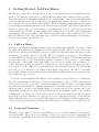
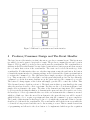
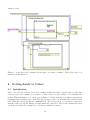
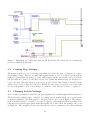
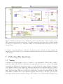
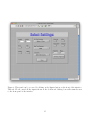
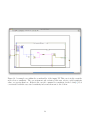
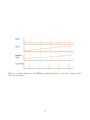
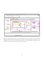
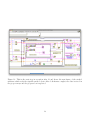
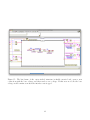
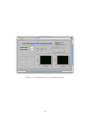
LabView Interface Development for a Low Frequency
Electron Epin Resonance Spectrometer
Rob Harrigan
Advisor: Dr. Hornak
20101-20102
Senior Project
February 21, 2011
1
Contents
1 Introduction
3
2 Background
2.1 Hyperfine Splitting . . . . . . . . . . . . . . . . . . . . . . . . . . . . . . . . . . . .
2.2 Magnetic Field Sweeps . . . . . . . . . . . . . . . . . . . . . . . . . . . . . . . . . .
3
4
5
3 Previous System and Interface Limitations
3.1 System Limitations . . . . . . . . . . . . . . . . . . . . . . . . . . . . . . . . . . . .
3.2 Previous Interface Limitations . . . . . . . . . . . . . . . . . . . . . . . . . . . . . .
5
5
6
4 Getting Started: LabView Basics
4.1 LabView Basics . . . . . . . . . . . . . . . . . . . . . . . . . . . . . . . . . . . . . .
4.2 Loops and Structures . . . . . . . . . . . . . . . . . . . . . . . . . . . . . . . . . . .
7
7
7
5 Producer/Consumer Design and The Event Handler
9
6 Getting Ready to Collect
6.1 Initialization . . . . . . . . . . . . . . . . . . . . . . . . . . . . . . . . . . . . . . . .
6.2 Creating Step Voltages . . . . . . . . . . . . . . . . . . . . . . . . . . . . . . . . . .
6.3 Changing Lock-In Settings . . . . . . . . . . . . . . . . . . . . . . . . . . . . . . . .
10
10
11
11
7 Collecting The Spectrum
7.1 Timing . . . . . . . . . . . . . . . . . . . . . . . . . . . . . . . . . . . . . . . . . . .
7.2 Sending Voltages . . . . . . . . . . . . . . . . . . . . . . . . . . . . . . . . . . . . .
7.3 Closing Connections . . . . . . . . . . . . . . . . . . . . . . . . . . . . . . . . . . .
12
12
13
13
8 Final Processing
13
9 Appendix
9.1 Quick Start Guide . . . . . . . . . . . . . . . . . . . . . . . . . . . . . . . . . . . .
14
14
2
Abstract
An interface was created to allow more control over a home built low frequency electron spin
resonance (LFESR) spectrometer. The interface was created using the LabView environment.
The new interface uses two voltages to drive the magnetic field which allows for more control
over the system and higher resolution sweeps can be performed in specific ranges of interest to
the user. The new interface also has a secondary panel which can control system settings on
the lock-in amplifier from the computer. This new interface has better functionality allowing
Dr. Hornak better control over his device and further advancing the science of LFESR.
1
Introduction
In this project an efficient user interface was created for the existing LFESR spectrometer built
by Dr. Joe Hornak. This spectrometer will further our knowledge of electron spin resonance
spectroscopy, which could one day be useful for detection of free radicals in patients. This new
interface allows more functionality and control including controlling settings on the lock-in from the
computer and using two voltage supplies to acquire high resolution sweeps of narrow magnetic field
regions. Free radicals have been seen as intermediates in the activation of some chemical carcinogens
as a product of the attack on the body due to ionizing radiation[1, 2]. It has been shown that free
radicals can be observed in cigarette tar extracts through ESR measurement [3]. Free radicals occur
naturally in metabolic pathways in the normal body but they also can be found associated with the
degradation of some drugs and poisons[1]. Other than diseases ESR spectroscopy can also be used
to evaluate the basic metabolic activity of cells, as well as studying different components of blood[1].
High frequency ESR systems are commercially available but would be harmful to animal subjects.
The study of LFESR is the exploration of one method of detecting free radicals in animals.
2
Background
This equipment is used for measuring free radicals which are unpaired electrons. The Pauli Exclusion
Principle says that no two electrons can have the same four quantum numbers[1]. This means that
electrons in the same atomic orbital must have a spin up or down. Any pair of electrons with
opposite spins will cancel to have no net magnetic moment. Not all electrons are paired however
so for some elements there will be electrons with a magnetic moment, meaning that if a magnetic
field is applied there will be an interaction. Electrons will align themselves with the direction of
the magnetic field. Larmor showed that a spinning frictionless magnet in magnetic field precesses
or rotates around the direction of the magnetic field similar to a top at a frequency known as the
Larmor frequency, ω is the angular Larmor frequency. This is the basis of magnetic resonance and
is given by ω = γH. Where γ is the gyromagnetic ratio, the ratio of magnetic moment of the
spinning magnet to its angular momentum and H is the magnitude of the magnetic field in Gauss.
From this and the definition of γ the governing equation of ESR can be derived:
hν = gβH
(1)
Where h is Planck’s constant, ν is the Larmor frequency, ω = 2πν, β is the Bohr Magneton and g is
a characteristic of a system, being 2 for electrons but closer to 2.0023 with relativistic corrections[1].
3
2.1
Hyperfine Splitting
In a system being examined through ESR with a magnetic field applied hyperfine splitting will
occur and can be seen in Figure 1. Splitting is caused by the interactions between the nuclear
magnetic moment and the spinning electron. As a magnetic field is increased on the system the two
spin states have different potential energies with respect to the external magnetic field. This will
continue until the basic equation of ESR (Equation 1) is satisfied and we will get an absorption of
energy, achieving resonance[1]. When the system is originally exposed to a small magnetic field this
will create an initial separation of the energy states. This is commonly due to the magnetic moment
of the nucleus of the atom which is very small in magnitude comparatively. This interaction will
create a small split in the energy levels even before the external magnetic field is applied. Figure 1
part B shows this as the two lines originating on the left side. When the field is applied this will
result in four energy levels but not all transitions are allowed. Transitions between a1 and b2 and
between b1 and a2 are allowed. Transitions from a1 to b1 and a2 to b2 are allowed but will not be
seen under experimental conditions[1]. So as the field is steadily increased there will be two lines
of absorption as the system resonates for each transition. The system can become more and more
complex if the nucleus has a spin other than 1/2 or if more than one nucleus is able to interact with
the electron[1].
Figure 1: (A) Spin splitting, (B) hyperfine splitting from nucleus interaction and the respective
absorption spectrums[1]
4
2.2
Magnetic Field Sweeps
In examining the main equation of ESR (Equation 1) it appears that either the magnetic field or the
frequency of radiation can be varied. Although this is true, magnetic field sweeps are almost always
used so that a lock-in amplifier can be used for detection. A lock-in amplifier, sometimes also known
as a phase-sensitive detector (PSD), is very good at extracting a signal of known frequency even
from very noisy environments. The amplifier uses a very low pass filter to create a narrow bandwidth
around the frequency of interest, known as the carrier frequency, to be able to better extract the
signal. The output of a PSD is also conveniently the first derivative of the absorption curve[1]. The
basic magnetic field sweep consists of just increasing the magnetic field slowly over time. When the
system achieves resonance there will be an absorption envelope that is either Gaussian or Lorentzian
depending upon the relaxation process which is occurring[1]. Another option is to use a modulated
sweep where the field is slowly increasing over time but also has faster variations up and down as
can be seen in Figure 2. The absorption curve will then show the rise and fall of absorption as the
field modulates. Figure 3 shows the effect of phase-sensitive detection on this system of rising and
falling absorption.
Figure 2: Modulated magnetic field sweep [1]
3
3.1
Previous System and Interface Limitations
System Limitations
Dr. Hornak built an ESR system designed for low frequency analysis of samples[2]. Although ESR
spectrometers are available for purchase commercially they use high frequency radiation that would
be harmful to an animal subject. This system is for researching the use of lower frequency radiation to avoid this effect and allow for this method to be used on animal subjects. The important
components of the spectrometer for this project are the control components. For this there are
two D-to-A converters. One is on the lock-in amplifier as described above which can also act as
a phase-sensitive detector and connects to the computer through an RS232 interface. The lock-in
5
Figure 3: (A) Modulation of the magnetic field sweep(without the net increase). (B) Signal received
from the system which is a combination of the absorption curve and modulation signal. (C) the
first derivative of the absorption curve obtained by phase-sensitive comparison of (A) and (B) [1]
amplifier is an SR-530 made by Stanford Research Systems and has an output voltage of ±10.24V
with 13 bits of resolution[6]. The second component is the board in the computer which is a National Instruments 6035E with 12 bits of resolution and also has an A-to-D converter with 16 bits of
resolution which could be used to do the phase sensitive detection in the software rather than using
the lock-in amplifier[4, 5]. These will be used to control a Kepco ATE 36-30M DC power supply
which will drive the electromagnet. This power supply uses a zero to one volt input for control.
Lastly the frequency generator is also controlled by the computer through a BCD connection.
3.2
Previous Interface Limitations
The previous interface was also built using LabView and was designed to simply sweep through the
entire magnetic field using one of the D-to-A converters and recording data along the way. This
means that the resolution of every sweep was the same and was matched to the resolution of the
D-to-A converter being used. Using this approach, the resolution is always the same and you have
to always sweep through an entire spectrum. A full sweep takes time and is not always necessary
for certain investigations.
6
4
Getting Started: LabView Basics
The first major task was to learn LabView and try to understand the code behind the previous
interface. The first step taken was to go through the tutorials included with the LabView package.
These tutorials were very helpful in giving the basics of the language. One of the most helpful parts
of the tutorials was at the end of each exercise an example was given for the user to complete on
their own and the correct solution is also available. This was helpful in writing small test programs
to understand how individual functions work. This was a strategy that I carried with me throughout
the project. Many test projects were written to test things such as how to set up the progress bar
so that it filled properly and a program which sends a single voltage to the NI board to understand
what settings to use for the desired result. These test programs can be found in the LabView folder
under the subfolder Tests. These programs could be used for further understanding of the interface
for anyone who wants to modify the code.
4.1
LabView Basics
LabView is a graphical programming language where everything visual including colors and borders
are significant in telling the programmer about the current program. LabView works on the basis
that you have a front panel which has controls and indicators and then behind that there is some
underlying code known as the block diagram. The block diagram is the essence of the graphical
program while the front panel just operates the underlying block diagram. Controls and indicators
are represented by the border of the function. If there is a thick colored border it is a control while
indicators have a thick white border with a thin colored border; See Figure 4 for an example of a
control (slide) and an indicator (numeric). Connections are made in the block diagram and functions appear as blocks. Different loops and structures are graphically represented by surrounding
the block code to be inside the loop. functions have inputs being wired to the left or occasionally
the top while outputs are wired from the right. This stems from the fact that code is executed from
left to right and top to bottom.
Colors are very meaningful in indicating the data type that is possessed in a wire or by a function.
The most important ones for this project being that blue is integer, orange is double, pink is string,
yellow is error, green is boolean, teal is a file reference number, purple is a visa resource name which
stores the port information for communicating with the lock-in and each port on the NI board. It
takes some time to get used to this graphical method of reading data types but over time can become
simpler than keeping track of them yourself as in traditional programming. Arrays are represented
by making the wire thicker for each dimension added. LabView automatically checks data types
and will grey out wires when they are connected to a port of the wrong data type. A LabView VI
will not run if there are any errors in the VI. When this occurs clicking the run button, which will be
a broken arrow, will bring up the errors list. Correcting these errors will then allow for the VI to run.
4.2
Loops and Structures
The basic loops necessary for this VI are the while loop, for loop, stacked structure, case structure
and event handler. These can be seen in Figure 5 These loops work as in basic programming but
are represented graphically as an area in the block diagram surrounded by the loop. The while loop
7
can be seen in Figure 4 and will continue to run while the wired condition is true or false. This
can be changed by clicking on the condition in the lower right hand corner to set it either equal
to stop on true or continue on true. The lower left corner holds the variable i which is the loop
iteration starting at zero. The loop in Figure 4 can be seen is wired as a stop on true condition
so when the ok button is pressed it will pass a true to the stop condition ending the loop and
quitting the VI since there is no block code to the right. The next important loop is a for loop.
This operates similarly except that it has a variable N in the upper left corner which is the number
of iterations to complete. When N iterations have been completed the loop quits. This loop is
represented graphically similar to a stack of pages surrounding the code to be executed. A stacked
structure is the next structure used in the interface and looks like a film strip surrounding the code
with a selector on the top. The selector at the top chooses what level in the stacked structure you
are viewing and the code executes in sequence. So level zero in the stack is executed and then
level 1 and so on. A case structure is the same as a case statement in programming but is used in
this interface as a substitute for an if statement. The case selector is on the left of the structure
halfway up and whatever this is wired to will determine what case is executed. The case structure
is used however with a boolean being wired to the case selector so that each case statement has
only two options, which can be selected at the top, either true or false. The event handler is the
final structure used and was the main improvement to the functionality of the new interface and
will be discussed in detail in section 7.
Some useful tools for debugging include the addition of breakpoints and the use of the wire probe
Figure 4: A basic VI which allows the user to change a displayed value and quits when the OK
button is pressed.
which allows for a user to see values within a wire at a breakpoint and the highlight execution tool.
The highlighting execution tool is similar to using the wire probe tool but works on all wires as the
program runs. This tool highlights each wire and displays the value as it is being sent through this
wire. This is a great tool for understand how loops work and execution order. This tool was most
useful when debugging the interface as a whole since the signals can be followed and it can be seen
exactly where the problem occurred.
8
Figure 5: Different loop structures used in the interface
5
Producer/Consumer Design and The Event Handler
The basic layout of the interface is what’s known as a producer consumer layout. This layout uses
two while loops and a queue to keep track of events. The producer consumer layout can be seen in
Figure 6. The top while loop is the producer and houses the event handler. The event handler is a
structure in LabView which waits for a user defined event such as a button press and then executes
the code under that section of the event handler. The event can be selected from the top of the
event handler. For this interface there are only three important events, the quit button, the button
to launch the inputs interface for changing settings on the lock-in and the acquire spectrum button
to activate the consumer loop. The quit button has a simple execution of stopping the producer
loop. This executes the code to the right to end the queue which will produce an error when the
consumer loop checks how many elements are in the queue and stop the consumer loop as well.
The button to change inputs on the lock-in will simply open the VI to control the lock-in. This
VI is discussed in more depth in section 6.3. The final event in this top event handler is the event
where the user has chosen to collect a spectrum. For this case the code is shown in Figure 6 and
simply adds an element to the queue. The value of the element is not important. The consumer
loop is repeatedly checking the number of elements in the queue and since it is equal to zero before
the user says to collect a spectrum the false case of the case statement in the consumer is executed
which is a blank case. Once the user adds an element to the queue the true case will be executed
which holds the code to acquire a spectrum and then exits the consumer loop upon completion.
The benefit of this structure is that large blocks of code which take an amount of time to execute
should not be left inside the event handler. The event handler will lock the front screen while the
code inside is being executed and this can be disconcerting to a user. This is a much cleaner form
of programming and allows for the abort button to be implemented which stops the acquisition
9
during a sweep.
Figure 6: A producer and consumer layout with a secondary consumer. This is the basic loop
structure for the interface.
6
6.1
Getting Ready to Collect
Initialization
Any code to the left of the producer and consumer architecture will be executed prior to the start
of the producer and consumer loop sequence so this is where we place all the code to initialize the
system. This initialization code can be seen in Figure 7. On the right the loop which represents the
beginning if the consumer can be seen. The upper portion of the code initializes the connection with
the lock-in and sets up the RS-232 communication. The lower portion of code starts a connection
with the NI Board, sets the timing, and then starts the connection. The resource names and errors
are then passed into the consumer loop for when acquisition is started.
10
Figure 7: Initializing the connections with the NI Board and the lock-in prior to starting the
producer-consumer architecture.
6.2
Creating Step Voltages
The first step in the process of collecting a spectrum is to create the array of voltages to be sent to
the stepping voltage. This is done using shift registers inside of a for loop that loops through the
number of points which are going to be sent. Shift registers are the arrows that can be seen on the
left and right side of the loop and these are used for passing information from one iteration of a
loop to the next. Once this array is created a zero is added as the last element so that the voltage
will be zeroed before closing the connection. Finally the four arrays are created to store the data,
two for each channel to store it as a string to be written to a file and as a double to be plotted.
6.3
Changing Lock-In Settings
Once a connection with the lock-in has been opened signals can be sent through the RS-232 interface.
The front panel settings can be controlled by sending various signals which can be found in the
lock-in user manual[6]. The front panel to control the lock-in can be seen in Figure 9. The interface
is an event handler inside of a while loop so the VI waits for a user input and then depending on the
button pressed sends the appropriate signal through RS-232 to the lock-in. An example can be seen
in Figure 10. This example is for the case that the user selects a sensitivity. If a valid sensitivity
11
Figure 8: This is the first part of the consumer loop and creates the array of sweep voltages on top.
The bottom section sets the base voltage, closes the connection and opens a new connection iwth
the other port on the NI board. The next column of blocks initializes the four arrays to store the
collected data.
is selected, one greater than zero, than the case shown executes. In this case the command for
sensitivity for the lock-in[6], G, is concatenated with the index for the selected sensitivity and sent
to the lock-in.
7
7.1
Collecting The Spectrum
Timing
Collecting a spectrum requires a series of events to occur sequentially. This is why a stacked
structure is used in the LabView environment to ensure that processes do not overlap. The timing
diagram shown in Figure 11 shows this sequence of events. First the voltage is stepped and then
a set amount of time is waited while the system and magnetic field stabilizes until the lock-in is
read. This process is repeated. The timing of the system can be fine tuned by changing the wait
time between readings. This can be changed by changing the constant 0.1 shown in Figure 12. This
is the number of milliseconds to wait after the stepping voltage is sent to the NI board before the
next frame which reads the lock-in is executed. The setting of 0.1 comes from the interrupt speed
12
of the NI board[4] so this timing setting only ensures that the NI board will not interrupt itself
before too quickly and skip voltages. The timing for the connection with the NI board is manually
set when the connection is opened also and is set to 10,000Hz. So if the wait time were reduced
below 0.1 voltages would be sent to the NI board more often than allowed by the timing set when
the connection was opened and the signal will be ignored. Increasing the wait time will allow more
time for the magnet to stabilize.
7.2
Sending Voltages
Figures 12 and 13 show the two frames of the stacked structure within the for loop which collects
each point in the spectrum. The for loop iterates for each point to be collected and then the
stacked structure executes. The first frame shown in Figure 12 sends the step voltage and then has
a wait built in to ensure that the system has adjustable timing. Being able to send this voltage
was a challenge. At first the DAQmx assistant was used but this allows no control over when the
connection is opened or closed. A resource reserved error will occur since the connection to the
base voltage cannot be closed and LabView cannot have two open connections to the same physical
device. The functions used are sub-functions of the DAQmx assistant and have the same end result
but allow control over when each step is executed allowing us to ensure that only one connection
is open at any one time and avoiding the resource reserved error. Once this frame completes the
system has a voltage and has been given time to stabilize, then the next frame will read the lock-in.
This is shown in Figure 13 where two commands are sent indicating to the lock-in that each channel
needs to be read. The lock-in will return each of the two values and then these can be stored in the
appropriate arrays. The arrays are sent to the next iteration with shift registers, the progress bar
is updated and the next iteration begins.
7.3
Closing Connections
After all iterations have been completed the outer sequential structure will execute the next frame
which can be seen in Figure 14. This frame simply closes the connection with the stepping voltage
so that a new connection can be opened in the next frame to zero the base voltage. The final frame
can be seen in Figure 15 and shows a new connection being opened with the base voltage and a
zero being sent. Once this is completed the interface moves on to post processing.
8
Final Processing
Once the spectrum is collected the text files are written. To do this the string arrays are converted
to a table string and then concatenated with a date stamp and written to the file selected by the
user. A waveform is then created using the data as the y input. The initial t is set to zero and
the dt is determined based on the number of points selected to allow for the t variable to be the
percent magnetic field sweep. The waveform is then plotted and the true constant means that the
consumer loop quits. At this point the user can press the quit button to stop the interface.
13
9
Appendix
9.1
Quick Start Guide
1. Turn on the system
2. Login with username:JoeAdmin Password:labview
3. open the folder in the top right corner of the desktop titled “LabView”
4. Double click on the file “LFESRSpectrometerFinal.VI”
5. When the file opens click the “RUN” button. (See Figure 17)
6. The interface is now running. Click on inputs if you wish to change settings on the lock-in
from the computer. Click Done when finished and return to the spectrometer interface.
7. Input the base voltage and number of points to be collected.
8. Set the correct resistance for the desired sweep range.
9. Double check all settings and finally click “Acquire”
10. The spectrum is now being collected but the user will be prompted as to where to save the
data files
11. A progress bar will show the progress through the scan. When the scan has completed press
quit to stop the interface from running. If you wish to stop a scan in progress press “Abort”,
not quit.
References
[1] M. A. Foster, Magnetic Resonance ain Medicine and Biology. Pergamon Press, 1984.
[2] J. P. Hornak, M. Spacher, and R. G. Bryant, “A modular low frequency esr spectrometer,”
Measurement Science and Technology, vol. 2, pp. 520–522, January 1991.
[3] L.-Y. Zang, K. Stone, and W. A. Pyror, “Detection of free radicals in aqueous extracts of
cigarette tar by electron spin resonance,” Free Radical Biology and Medicine, vol. 19, no. 2,
pp. 161–167, 1995.
[4] National Instruments, NI 6034E/6035E/6036E Family Specifications, December 2005.
[5] National Instruments, Low-Cost E Series Multifunction DAQ, 2006.
[6] Stanford Research Systems, 1290-D Reamwood Avenue Sunnyvale, Ca 94089, Model SR530
Lock-In Amplifier, 2.3 ed., June 2005.
14
Figure 9: This panel can be accessed by clicking on the Inputs button on the front of the interface.
This sub VI can control all the inputs shown on the lock-in and clicking done will return the user
to the front panel of the interface.
15
Figure 10: A example case within the event handler of the inputs VI. This case is in the event the
user selects a sensitivity. The case statement only activates if the user selects a valid sensitivity
value, one greater than zero. If that is the case the command for sensitivity for the lock-in[6], G, is
concatenated with the associated sensitivity index and then sent to the lock-in.
16
Figure 11: A timing diagram for the LFESR experiment showing the order that commands will be
sent from the interface.
17
Figure 12: The structure shown is a stacked structure inside a for loop inside a stacked structure.
The inner stacked structure sends the voltage to the NI board, then reads the lock-in as can be seen
in Figure 13. This occurs for every iteration in the for loop. After both frames complete the data
is stored in the proper arrays and the progress bar is updated.
18
Figure 13: This is the next step in execution after 12 and shows the next frame of the stacked
structure which reads the signal from the lock-in. After both frames complete the data is stored in
the proper arrays and the progress bar is updated.
19
Figure 14: After all the iterations of the for loop are completed the next frame of the outer stacked
structure executes which can be seen here and simply closes the connection with the stepping voltage
since a zero has already been sent as the last element in the array of stepping voltages.
20
Figure 15: The last frame of the outer stacked structure is finally executed and opens a new
connection with the base voltage and then sends a zero voltage. If this were not done the base
voltage would remain even after the interface was stopped.
21
Figure 16: After all of the iterations have been completed and the spectrum has been collected the
data is saved to a file that the user selects with a date stamp at the top and then the data is plotted
as a function of the percent magnetic field sweep.
22
Figure 17: Click this button to start the Program
23