Download STATWEAVE Users` Manual

S TAT W EAVE Users’ Manual
Russell V. Lenth
University of Iowa
January 30, 2012
Contents
1
Introduction
2
2
Installing S TAT W EAVE
2
3
Running S TAT W EAVE
3.1 Graphical interface . .
3.2 Command line . . . . .
3.3 Languages and engines
3.4 Order of processing . .
4
5
.
.
.
.
.
.
.
.
.
.
.
.
.
.
.
.
Making a source file
4.1 LATEX source files . . . . . . .
4.2 ODT source files . . . . . . . .
4.3 Auto-correction caution . . .
4.4 Summary of S TAT W EAVE tags
.
.
.
.
.
.
.
.
.
.
.
.
.
.
.
.
.
.
.
.
.
.
.
.
Setting options in the source file
5.1 Option format . . . . . . . . . . . .
5.2 Options for code-chunk processing
5.3 Options for code listings . . . . . .
5.4 Options for output listings . . . . .
5.5 Options for graphics . . . . . . . .
.
.
.
.
.
.
.
.
.
.
.
.
.
.
.
.
.
.
.
.
.
.
.
.
.
.
.
.
.
.
.
.
.
.
.
.
.
.
.
.
.
.
.
.
.
.
.
.
.
.
.
.
.
.
.
.
.
.
.
.
.
.
.
.
.
.
.
.
.
.
.
.
.
.
.
.
.
.
.
.
.
.
.
.
.
.
.
.
.
.
.
.
.
.
.
.
.
.
.
.
.
.
.
.
.
.
.
.
.
.
.
.
.
.
.
.
.
.
.
.
.
.
.
.
.
.
.
.
.
.
.
.
.
.
.
.
.
.
.
.
.
.
.
.
.
.
.
.
.
.
.
.
.
.
.
.
.
.
.
.
.
.
.
.
.
.
.
.
.
.
.
.
.
.
.
.
.
.
.
.
.
.
.
.
.
.
.
.
.
.
.
.
.
.
.
.
.
.
.
.
.
.
.
.
.
.
.
.
.
.
.
.
.
.
.
.
.
.
.
.
.
.
.
.
.
.
.
.
.
.
.
.
.
.
.
.
.
.
.
.
.
.
.
.
.
.
.
.
.
.
.
.
.
.
.
.
.
.
.
.
.
.
.
.
.
.
.
.
.
.
.
.
.
.
.
.
.
.
.
.
.
.
.
.
.
.
.
.
.
.
.
.
.
.
.
.
.
.
.
.
.
.
.
4
4
4
5
6
.
.
.
.
6
7
9
11
11
.
.
.
.
.
12
12
12
13
14
14
6
Programming statements
15
6.1 Code reuse and argument substitution . . . . . . . . . . . . . . . . . . . . . . 15
6.2 Including external files . . . . . . . . . . . . . . . . . . . . . . . . . . . . . . . 17
6.3 Defining new languages . . . . . . . . . . . . . . . . . . . . . . . . . . . . . . 18
7
Configuring and customizing S TAT W EAVE
18
8
Acknowledgements
19
1
1
Introduction
S TAT W EAVE is an extension of some previous literate-programming packages (S WEAVE,
SAS WEAVE, and ODF W EAVE) for statistics. Its intent is to provide portable software that
can integrate code and documentation for a large variety of statistical (and nonstatistical)
languages and file formats, and also to provide for extensibility so that a user can add
more file formats and languages.
S TAT W EAVE is written in Java, providing easy portability across platforms. As currently implemented, S TAT W EAVE has only a command-line interface, but a graphical interface could be easily added. A Java virtual machine (JVM) is already installed on most
people’s systems, and the decision to use Java also separates S TAT W EAVE from requiring
the user to have any particular one of the statistical packages it supports.
In its current implementation, the supported languages include R, SAS, Stata, S-Plus,
Maple, LATEX, DOS, and UNIX; and more can easily be added. The currently supported file
formats are .tex (using an extension of S WEAVE’s LATEX syntax) and .odt (the Open Document Format XML specification currently implemented in OpenOffice). The probable
next developments for file formats would be Word 2007’s .docx format, and extending
the .tex format to support S WEAVE’s noweb syntax.
To use S TAT W EAVE, one prepares a source file in the same basic format as the intended output file. Computer code is added to this file, and marked in some way so that
S TAT W EAVE can tell that it is code in a certain language. These marked blocks of code are
called “code chunks.” Processing via S TAT W EAVE involves extracting and running the
code chunks in the appropriate program(s), and creating an output document that contains all the materials in the source file, but embedding the code listings, output listings,
and any graphics produced in place of the code chunks. S TAT W EAVE figures out which
programs it needs to run, and runs them in order of first appearance in the source file.
Section 2 outlines how to install S TAT W EAVE on your system. Section 3 explains how
to run S TAT W EAVE from the command line, and the command-line options that are available. In Section 4, we describe how to prepare a source file for S TAT W EAVE. Section 5
details the various options that can be specified in the source file for controlling how the
code chunks are processed and displayed. S TAT W EAVE uses a configuration file that defines defaults for processing, specifies what languages are supported, provides paths to
these languages’ implementations on the local machine, etc. Section 7 explains the construction of this file. Finally, S TAT W EAVE is designed to be extensible, and a separate
document1 describes the Java class structure and how various interfaces can be implemented and configured to add support for new languages or file formats.
2
Installing S TAT W EAVE
All necessary components of S TAT W EAVE are provided in a single file, statweave.jar.
This is a Java archive file.2
1 This
manual is forthcoming
2 Because it has the same format as a ZIP archive, it is possible that your web browser will want to unpack
it. Don’t let that happen: keep it as a JAR file.
2
Before installing S TAT W EAVE, you should consider the following items, and gather
the necessary information.
• Decide in what directory on your system you want to install S TAT W EAVE.
• Decide where on your system you want to install the statweave script (the system
command that runs S TAT W EAVE). If you will want to run S TAT W EAVE from the
command line, this should be a directory that is included in your PATH environment
variable (e.g., /usr/local/bin on most Unix or Linux syatems). Many Windows
and Mac OS users will want to use the graphical interface, in which case we recommend just putting it in the installation directory.
• Will you use LATEX with S TAT W EAVE? If so, there is a LATEX package file that will
be copied to your system. Decide where you want this file. Generally, it should be
put in a directory where LATEX can find it. On many systems, these directories are
in a TEXINPUTS environment variable; on other systems (e.g. MikTEX on Windows),
these are specified in an Options menu (e.g., the “Roots” tab in MikTEX).
• Will you use OpenOffice Writer with S TAT W EAVE? If so, there is a template file that
will be copied. The best location is the default templates directory—see the menu
Tools/Options/Paths.
• Do you have permission to write to the above directories? If not, you may need
someone’s help, or to log in as a root user or administrator.
• For each piece of software you plan to use with S TAT W EAVE, you will need to configure S TAT W EAVE to use it. In Unix, Linux, and MacOS systems, most software is
installed to be already accessible from the command line—in which case the default
configuration for a language will often work. In Windows, you often have to specify exactly where the application’s .exe file is installed. The setup procedure allows
you to browse your system to find these places.
• S TAT W EAVE requires Java to be installed on your system, and it must be version
1.5 or later. You probably already have it, so just try the directions below. If they
fail, then you will need to install or update Java. For all but MacOS systems, it is a
free download from java.sun.com: follow the link for downloading J AVA SE; it is
sufficient to install the Jave runtime environment (JRE). For Mac OS systems, do a
software update.
Now, to install S TAT W EAVE on most systems, all you need to do is double-click on the
icon for statweave.jar;3 if that doesn’t work, you may use the command
java -jar statweave.jar
3 You
might as well move statweave.jar to the desired installation directory first. This is not required,
but the installation procedure copies it there anyway.
3
You will see a series of message boxes and dialog windows, where you are prompted
for answers to the questions discussed above. The last part of this process, you will
see a dialog window that lists available languages. For each one that you want to use
with S TAT W EAVE (and that is installed on your system), select that language and click on
“(Re)Configure.” This will show a dialog window for editing the configuration keys associated with that language. Depending on the language, one (but not both) of the .binary
or the .args keys (i.e., command or arguments) may need to be modified to match your
system installation—click on the “Modify” button to change a value. If you need to replace part of the arguments to a command with a file or directory location, use the mouse
to select that portion of the arguments first; then you will be able to browse your system
to find a suitable replacement.
3
Running S TAT W EAVE
3.1
Graphical interface
To use the graphical interface, double-click on the script statweavegui4 in the installation
directory. Alternatively, you may run the command
statweave --gui
from a console. From the resulting dialog, you may do most S TAT W EAVE-related operations. Its File menu provides for browsing for a source file, and exiting. Its Options menu
allows you to specify options (comparable to the command-line options listed in Section 3.2), or to modify S TAT W EAVE’s configuration. There is a “Run” button for running
S TAT W EAVE on the currently selected file.
If you know how to do this on your system, you may set up a menu shortcut for—or
associate S TAT W EAVE source files with—statweavegui (under Windows, use statweavegui.bat).
This script will be found in the installation directory.
3.2
Command line
To run S TAT W EAVE, the command line is
statweave [option(s) ] file
where file is the name of the source file. The possibilities for option(s) are described
shortly. S TAT W EAVE determines the file format based on its name and extension, which
in turn is delineated in the configuration file (see Section 7).
The options may include any or none of the following; what is default is again determined by the configuration file.
4 Double-clicking
on the icon for statweave.jar (in the installation directory) will also work; however,
some languages do not work right if you start S TAT W EAVE this way, unless the installation directory is the
the PATH.
4
--weave Make a complete document containing all the writing in the source file, and the
code chunks replaced by code listings plus any output and graphics produced by
running the code. (Note that options within the source file may be used to selectively suppress or relocate these elements when you don’t want them displayed in
the standard manner.)
--tangle Extract the code chunks into separate files, one for each language used in the
document. Do not make an output document.
--config cfgfile Read configuration information from the specified file, rather than
the default one.
--custom custfile After the regular configuration information is loaded, read additional configuration information from the specified file. Entries in this file will supplement or replace those in the configuration file.
--target ext Specify the type of output file. Currently, this applies only to a tex source,
where the targets could be tex, dvi, or pdf; the latter two entail further processing
of the tex target.
--cleanup Delete all intermediate files created in the weaving process.
--tidyup Delete only certain intermediate files, as defined by the file-format driver (usually, this will mean keeping graphics files and deleting the rest).
--keepall Do not delete any intermediate files.
--dryrun Do not evaluate any code chunks. This would be useful, for example, for debugging the LATEX portion of a source file without running any of the statistical code
embedded in it.
--gui Brings up the graphical interface to S TAT W EAVE.
Various results will be displayed as S TAT W EAVE runs. If there are errors, any cleanup
operations are aborted as well so that you may examine intermediate files and hope to
find the errors.
3.3
Languages and engines
In this manual, a “language” refers to a computer language used for statistical or other
analysis, and an “engine” is the program that implements the language. Often, languages
and engines have the same name, e.g. “SAS.” However, an engine can potentially run
more than one language. For example, code chunks in languages SAS and IML are both
run in the SAS engine. If code chunks for two or more languages that share the same
engine appear in the source file, they are collected together into one code stream that is
subsequently run by that engine. For example, if IML chunks are insterspersed with SAS
chunks, they are all processed as a single SAS program.
5
In some cases, it is useful to make distinctive use of multiple languages that share
an engine; for example, we can set options specifying that the SAS code and results are
formatted differently than the IML code and results. It is possible to define new languages
on the fly; see Section 6.3 for details.
3.4
Order of processing
When you run S TAT W EAVE, the chunks of code are extracted from the source file and
assembled into separate code files, one for each engine required by the embedded code.
If tangling is requested, we are now done. If we are weaving, the code files are run in
order of first appearance in the source file, then the results are collected and embedded in
the output document.
It is possible that one engine will produce results that are needed by another engine—
say, by writing data to a file. Since engines are run in order of first appearance, that will
work fine as long as the first code chunk for the second engine appears after the first
code chunk for the second engine. If files are passed back and forth, you need to use the
restart option to start a new instance of an engine with its own code file. See Section 5.
4
Making a source file
To use S TAT W EAVE, the primary activity is preparing a suitable source file. This file needs
to contain instructions to delineate code chunks, as well as possibly specifications of various options for how they are processed and displayed, and/or instructions for including
certain parts of the output. We will use the term “tag” to refer to a portion of the sourcefile content that signals S TAT W EAVE to give it special treatment. Here are the tags that
can be included in the source file, regardless of its file format:
• Tags for delineating code chunks
• Tags for specifying options for processing a particular code chunk
• Tags that specify global options that apply to all code chunks
• Tags that provide language-specific options that apply to all chunks in a given language
• Tags for evaluating an expression and embedding the results within a paragraph of
the document
• Tags for saving and re-using code chunks, perhaps with argument-substitution—
essentially a mechanism for defining macros
• Tags for saving and restoring portions of the output of code chunks—the output,
code listing, and graphs.
6
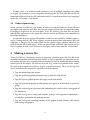
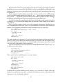
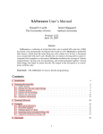
Figure 1: Demo source file demo-swv.tex in LATEX format
\documentclass{article}
\begin{document}
\SASweaveOpts{prompt="$ "}
\section{StatWeave example using SAS}
Let’s read in some data and copy it into a matrix in IML:
\begin{SAScode}
data chickwgt;
infile "chickwgt.txt" firstobs = 2;
input weight time chick diet;
\end{SAScode}
\begin{IMLcode}
proc iml;
use chickwgt;
read all into A;
\end{IMLcode}
We have read-in \IMLexpr{nrow(A)} observations and \IMLexpr{ncol(A)} variables.
Let’s do an analysis.
\begin{SAScode}{label=mixed,saveout}
proc mixed;
class diet chick;
model weight = time diet;
random chick(diet);
\coderef{hidden}{ods select tests3;}
\end{SAScode}
The output is as follows:
\recallout{mixed}
\end{document}
The main part of the S TAT W EAVE software reacts to the presence of these tags. The software specific to different file formats are responsible for defining how these tags are specified in the source file, finding the tags, and communicating the information to the main
program.
In its current implementation, S TAT W EAVE supports two file formats: LATEX and OpenDocument text (ODT). The following subsections describe how to use S TAT W EAVE tags
in each of these formats. They also describe the basic style we recommend for future extensions to other file formats. File formats that use markup should use a comparable style
to that defined for LATEX sources below. Future extensions to WYSIWYG (“what you see
is what you get”) source files should define tags comparably to the way they are defined
below for ODT files.
4.1
LATEX source files
7
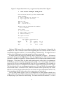
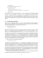
Figure 2: Output document demo.pdf generated by source file in Figure 1.
1
StatWeave example using SAS
Let’s read in some data and copy it into a matrix in IML:
$ data chickwgt;
$
infile "chickwgt.txt" firstobs = 2;
$
input weight time chick diet;
IML> proc iml;
IML>
use chickwgt;
IML>
read all into A;
We have read-in 578 observations and 4 variables.
Let’s do an analysis.
$ proc mixed;
$
class diet chick;
$
model weight = time diet;
$
random chick(diet);
The output is as follows:
The Mixed Procedure
Type 3 Tests of Fixed Effects
Num
Den
Effect
DF
DF
F Value
time
1
527
2468.49
diet
3
46
6.28
Pr > F
<.0001
0.0012
Ordinary LATEX source files use markup to define how the document is formatted; for
example, the \section macro is used at the beginning of a new section, and the itemize
environment together with the \item macro defines a bulleted list. It is logical to use a
similar style of markup to insert tags into an S TAT W EAVE source file.
A simple source file using SAS and IML code is illustrated in Figure 1. It illustrates
most types of tags for the LATEX format. Near the beginning, the \SASweaveOpts macro
specifies an option that applies to all code chunks in SAS (but not to code chunks in other
languages). A few lines later, the first code chunk appears in the SAScode environment.
S TAT W EAVE uses the characters that precede the string “code” to determine that the language is SAS. Next is a code chunk for IML (the IMLcode environment). This example assumes that S TAT W EAVE is configured so that IML is another language for the SAS engine.
The line after the IMLcode environment contains two \IMLexpr macros; the arguments to
these macros will be evaluated in IML, and these macros will be replaced by the results.
(By the way, in SAS, it does not make sense to evaluate an expression outside of PROC IML,
so it is important for IML to be active when expressions are embedded.)
The last code chunk (again a SAScode environment)
has some options added; these
1
assign a label to the code chunk and instruct S TAT W EAVE to remember the output instead
of displaying it just below the code listing. The code chunk itself contains a \coderef
8
macro. Normally, this is used to reuse the code in a previous code chunk. In this instance,
we reuse a rather trivial, built-in chunk named hidden that simply adds the supplied
argument (in this case an ods statement) invisibly to the code that is executed. This is
handy, especially in SAS, for selecting only certain parts of the output.
After this last SAScode environment is a line of text for the document. This is followed
by a \recallout macro that requests we now display the output that we had saved under
the label “mixed.”
The resulting document obtained by running S TAT W EAVE on this source file is displayed in Figure 2. The text elements in the original document are exactly as was entered
in the source file; but the code chunks and macros containing S TAT W EAVE tags have been
suppressed or replaced with formatted code listings and output, if any. The initial SASspecific option caused the lines in the listing of SAS code to be preceded by the $ character
and a space. That option was SAS-specific, though, so the lines of IML code are preceded
by the default prompt, which is the language name followed by “> ”. We could have
used “SAS” in place of “IML” in the source-file tags, and exactly the same results would
have been obtained except for the prompt strings. If any output had been generated by
these code chunks, it would have been displayed immediately after the code listings.
We verify that the \IMLexpr macros now contain the actual number of observations
and variables. The code listing for the final chunk reverts to the dollar-sign prompt. Note
that the \coderef line is not displayed in there. The requested portion of the output
is shown where it was requested by the \recallout macro. Had we not used that, we
would not have been able to put the intervening narrative between the code listing and
the output.
4.2
ODT source files
OpenOffice is a freely available, open-source office suite that includes a word processor,
spreadsheet, database, etc. The word processor, OpenOffice Writer, is an example of a
WYSIWYG interface. In OpenOffice Writer, the same functionality as LATEX markup is implemented in a style menu; for example, a “heading 1” style is comparable to a \section
macro in LATEX. Accordingly, our standard design for ODT source files uses custom style
markings as tags for the various S TAT W EAVE elements. This design has the additional advantage that our custom styles can include special colors and fonts to make the presence
of S TAT W EAVE tags easily noticeable.
To create an ODT source file for S TAT W EAVE, simply open a new document based on
the SWstyles template that accompanies S TAT W EAVE. (Or after starting the new document, load the template via the style menus.) This template defines styles that correspond
to all the needed tags in S TAT W EAVE. You can find them in the “custom styles” listings
for paragraphs and character formats.
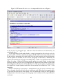
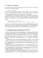
To illustrate, Figure 3 shows a screen shot of an ODT equivalent of the LATEX source
file shown in Figure 1. In this figure, the current position of the cursor is at the end of
the last line of the IML code. Note that the style selector (to the left in the lower part of
the toolbar) displays that the style here is SWcodebody. This is a paragraph style that is
used for each line of each code chunk; as provided, this style displays in monospace black
fonts with a light blue background. Everything that is formatted like that in Figure 3 is
9
Figure 3: ODT source file demo-swv.odt comparable to the one in Figure 1.
in the SWcodebody paragraph style, and that is how S TAT W EAVE can tell that they are
code-chunk lines.
At the beginning of each code chunk is a single paragraph in SWcodehead style, displayed in white text with a dark blue background. Most code chunks should be preceded
by one of these paragraphs (if a code chunk is in the same language as the previous one,
and no options are needed, the SWcodehead paragraph is not needed). Minimally, the
code header contains the language name followed by a colon. Any options for that chunk
follow the colon. Global or language-specific options are quite similar to code-chunk
headings, only they use the SWopts paragraph style, displayed with yellow text on a dark
blue background. The first line in the document is a SAS-specific option. A global option
that applies to all code chunks would have been similar, but without the “SAS:” at the
beginning.
In-line evaluation of expressions is accomplished using the SWexpr character style.
This is the only S TAT W EAVE style that is a character style rather than a paragraph style,
so you will not find it on the same menu. They are displayed as blue text on a light-blue
background, and to enter one, give the language name, a colon, and the expression to be
evaluated.
10
There are two more to go. The recalled code that was accessed using \coderef in the
LATEX example is implemented using the SWrecall paragraph style. Give the label (in
this case, “hidden”), and any arguments enclosed in curly braces. It is displayed with
a light-yellow background. Recalled output is obtained using the SWrecall paragraph
style, displayed with a coral background. Give the keyword “output:” followed by the
label for the output. Saved code listings and graphics are recalled in the same way, using
the keywords “code:” and “fig:” respectively.
The provided template includes two other styles named Winput and Woutput. These
define the styles to be used for code listings and output listings in the output document. The output document will inherit these styles. Thus, while they are not needed
for S TAT W EAVE tags, you can modify these styles according to how you want code and
output listings to be formatted in the output document.
4.3
Auto-correction caution
One issue peculiar to WYSIWYG word-processors is that they quietly modify certain
things that you enter. For example, quotation marks are changed to opening and closing quotes, and hyphens in certain contexts are changed to en dashes. This is problematic
because minus signs and quotes are important elements of computer code. S TAT W EAVE
specifically looks for and reverses the most common of these, but it is easy for some other
auto-correct artifact to pass through to the program that is run. Thus, you may want to
disable or severely limit auto-formatting when you prepare the source file.
4.4
Summary of S TAT W EAVE tags
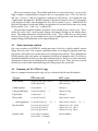
Here is a compact reference to the tags we have discussed for the two file formats.
Tag type
LATEX source file
ODT <style>
Code chunk
\begin{lang code}{opts } . . .
\end{lang code}
<SWcodehead>lang :opts ,
<SWcodebody>...
Global options
\weaveOpts{...}
<SWopts>...
Lang-specific opts
\lang weaveOpts{...}
<SWopts>lang :...
Expression
\lang expr{...}
<SWexpr>...
Reuse code
\coderef{label }
<SWcoderef>label
. . . with arguments \coderef{label }{...}{...}
<SWcoderef>label {...}{...}
Recall results
\recallcode{label }
\recallout{label }
\recallfig{label }
<SWrecall>code:label
<SWrecall>out:label
<SWrecall>fig:label
Include a file
\weaveIn{filename }
\weaveIn{< filename }
(not available)
11
5
Setting options in the source file
As explained earlier, options may be specified to determine how a code chunk is processed, what is displayed, how it is formatted, and so forth. The options may be specified
either at the beginning of the code chunk, in which case they apply only to that chunk;
or in a global or language-specific options specification, in which case they apply to all
subsequent chunks or until overridden by other options. This section describes the options that are available. Note that some options are available only for certain file formats
or certain languages. As new drivers are added, the available options may expand.
5.1
Option format
Both LATEX and ODT files require essentially the same format for options: a commadelimited list in the format
key1=value1,key2=value2, key3 = value3, ...
where the key s are the option names. If desired, extra spaces may be added around
equal signs and commas. If a value must include a comma or a space, it may be enclosed
in double quotes ("..."); and if quotes within quotes are needed, consecutive quotes are
interpreted as a quote character; for example, prompt = "-""- " sets the prompt string
to -"-, followed by a space.
Many options are boolean (values are TRUE or FALSE). These values may be abbreviated
T and F. There is an even terser form for a boolean option: just the keyword with no
value is taken as TRUE, and an exclamation point before the keyword sets it to FALSE.
For example, an option list of fig,!echo is equivalent to fig=TRUE,echo=FALSE. Another
thing to know: if S TAT W EAVE or an associated driver tries to test an option and it is found
to not even exist, it is taken as FALSE.
Finally, it is possible to remove an option altogether by preceding its name with a
hyphen. For example, we may have set a global option of prompt="> " but you later
want to use the default prompt; then include -prompt in the option list.
5.2
Options for code-chunk processing
eval (boolean) If TRUE, the code will be run by the appropriate program; if FALSE, it is
only listed (assuming echo is TRUE).
restart (boolean) If TRUE, and there have been previous code chunks for the same engine, a new code stream is started for that engine that will be run separately, after
the previous ones.
label (string) The value is assigned as a label that can be used later to reference the code
chunk or some result produced by it. If a label is not provided, the label lastchunk
is assigned and remains valid until another unlabeled chunk appears.
The factory default is eval=TRUE and the others undefined.
12
5.3
Options for code listings
echo (boolean) If TRUE, the code chunk is listed; if FALSE, it is not
prompt, prom, ompt, cont (string) If it is defined, the value of prompt is appended to
the beginning of each line of the code listing. If undefined, prompt is formed by
concatenating the values of prom and ompt. prom defaults to the current language
name, and ompt defaults to “> ”. For example, in a SAS code chunk, by default
each code-listing line is preceded by “SAS> ”. Note that prom and ompt have no
effect when prompt is defined; you may un-define prompt using -prompt. The cont
option specifies a separate prompt to use for continuation lines. This works only
with language drivers that support it. (As of January 2012, this is Stata only, and not
yet R). If cont is not specified, the current prompt is used.
savecode (boolean) Suppresses the code listing, but saves it for later recall using the
chunk label.
showref (boolean) If TRUE, reused code is displayed in the code listing; if FALSE, it is
hidden.
codestyle (string) You may use this option to specify a paragraph style name (for ODT
files) or environment name (for LATEX files) to be used for formatting the code listing.
The default is Winput. In an ODT file, the named style should be defined in the
source document; the Winput style is provided in the template SWstyles.ott that
comes with S TAT W EAVE. For a LATEX file, this must be defined using the \DefineVerbatimEnvironment or \RecustomVerbatimEnvironment macros in the fancyvrb
package; the Winput environment is defined in the file StatWeave.sty that comes
with S TAT W EAVE.
codefmt (string; LATEX-specific) The value of codefmt is inserted as optional arguments
for the verbatim environment that is used for displaying the code listing—thus allowing you to change the formatting in a variety of ways. For example,
codefmt = "formatcom=\color{blue}, frame=single"
will alter the formatting so that the code listing is in blue, and surrounded by a
box. For details on what is possible, see the documentation for the LATEX package
FANCYVRB .
beforecode, aftercode (string, LATEX-specific) If specified, these strings are inserted in
the LATEX result file just before and just after each code listing.
The factory defaults are echo=TRUE, eval=TRUE, showref=FALSE, and codestyle=Winput;
the rest are left undefined. These can be changed in the configuration file.
13
5.4
Options for output listings
hide (boolean) If TRUE, output is not displayed; if FALSE, output is displayed.
results (file-format-dependent) In a LATEX source file, results=tex specifies that the
output is expected to be in LATEX format. In an ODT source file, results=xml is
used when the code produces output containing XML tags, such as a table.
saveout (boolean) Suppresses the code listing, but saves it for later recall using the chunk
label.
loose, tight (boolean) These options control the way in which blank lines are compressed. If both options are false, (1, 2, 3, 4, 5, 6, . . .) consecutive blank lines are replaced by (1, 1, 1, 2, 2, 3, . . .). If tight is TRUE, these are replaced by (0, 1, 1, 1, 1, 2, . . .);
otherwise, if loose is TRUE, no compression of blank lines is performed. In all cases,
all blank lines that precede the first line or follow the last line of output are removed.
Tight spacing might be preferred if you want to remove blank lines that precede table headings (such as are produced by SAS); the down side is that if two tables are
separated by only one blank line, they will be squashed together.
outstyle (string) You may use this option to specify a paragraph style name (for ODT
files) or environment name (for LATEX files) to be used for formatting the verbatim
output listing. The default is Woutput. If the results option is other than verbatim,
this option has no effect. In an ODT file, the named style should be defined in the
source document; the Woutput style is provided in the template SWstyles.ott that
comes with S TAT W EAVE. For a LATEX file, this must be defined using the \DefineVerbatimEnvironment or \RecustomVerbatimEnvironment macros in the fancyvrb
package; the Woutput environment is defined in the file StatWeave.sty that comes
with S TAT W EAVE.
outfmt (LATEX-specific) The value of outfmt is inserted as optional arguments for the
environment that is used for displaying the output listing—thus allowing you to
change the formatting in a variety of ways. See more discussion under codefmt
above.
beforeout, afterout (string, LATEX-specific) If specified, these strings are inserted the
LATEX result file just before and just after each output listing (whether or not it is
verbatim).
The factory defaults are hide=FALSE, outstyle=Woutput, and the rest are undefined. These
can be changed in the configuration file.
5.5
Options for graphics
fig (boolean) If TRUE, we expect the code to produce a graph; by default, it will be
displayed below the output listing. Currently, S TAT W EAVE only provides for one
graph from each code chunk. If more than one graph is actually produced by that
14
chunk, it may cause an error; if not, what is displayed may be the first or the last
one produced, depending on the software.
width (dimension) Specify the width of the constructed figuer. This is used by S TAT W EAVE
when it sets up a file or graphics output stream for it. The value may end in in, cm,
mm, pt, or px to specify inches, centimeters, millimeters, points, or pixels. If no units
are given, S TAT W EAVE makes a reasonable guess based on the size of the number.
If no width is specifies, the default is 6 inches (or the equivalent in other units).
figfmt (string) If specified and fig is TRUE, this forces the graphics format to be the specified value. The valid values are eps, gif, jpg (or jpeg), pdf, png, ps, or tif. You
get an error if the format is not supported for both the statistical language and the
target file format.
height (dimension) Same as width, but for the height of the figure.
dispw (dimension) Set the displayed width of the figure as it is to appear in the output
document. If this is not specified, the value of width is used.
disph (dimension) Set the displayed height of the figure as it is to appear in the output
document. If this is not specified, the value of height is used.
scale (number) Set a scale factor for expanding or contracting the figure from its original
width and height. If not give, a value of 1 is assumed.
savefig (boolean) Suppresses the display of the figure, but saves it for later recall.
beforefig, afterfig (string, LATEX-specific) If specified, these strings are inserted the
LATEX result file just before and just after each figure.
A note on scaling: Ordinarily, you should specify only one of the options dispw, disph,
or scale. If scale is defined, dispw and disph are ignored. Specifying only dispw is
equivalent to setting scale equal to dispw/width. If both dispw and disph are defined,
they are both used, and this will distort the shape of the graph when they are not in the
same proportion as width and height.
6
Programming statements
This section describes some S TAT W EAVE constructs that in essence provide programming
statements within the source file.
6.1
Code reuse and argument substitution
A code chunk may be saved under a label, and recalled later using the reuse-code tag for
the file format in question (see Section 4.4). If no label is provided, a code chunk may still
be recalled under the label lastchunk until a new code chunk is defined.
15
Recalled code may or may not be displayed in the code listing, depending on whether
the option showref is true or false. By default, it is false, meaning that recalled code is not
displayed. You may force a particular chunk to be displayed by preceding its label with
an asterisk (*).
Finally, argument substitution is provided in a manner similar to that of TEX macros.
If the saved code chunk contains the strings #1, #2, . . . , those strings are replaced by the
first, second, . . . arguments provided with the reuse-code tag. Both the ODT and LATEX
file formats provided specify that these arguments be enclosed in braces.
S TAT W EAVE provides a predefined (and rather trivial) code chunk named hidden that
is simply #1. It is very useful for hiding code that you don’t want echoed; see the following example.
Here is a LATEX example of code reuse with argument substitution. Imagine that we
have a document with SAS code, and we want to import several datasets with various file
formats. The appropriate code for this will be entered early in the source file:
\begin{SAScode}{label=import, !eval, !echo}
proc import
filename = #1.#2
out = #1
dbms = #3 replace;
\end{SAScode}
The code contains the strings #1, #2, and #3 for later substitution with the root name of
the file (as well as the name of the dataset created), its extension, and the delimiter used.
The code chunk has the label import; we disabled both evaluating the code (which would
cause an error!) and echoing it to the document.
Later in the document, we want to read in a comma-delimited file named beans.csv;
so, include this code chunk:
\begin{SAScode}
\coderef{import}{beans}{csv}{csv}
proc print data=beans;
\end{SAScode}
This is equivalent to embedding these two code chunks:
\begin{SAScode}{!echo}
proc import
filename = beans.csv
out = beans
dbms = csv replace;
\end{SAScode}
\begin{SAScode}
proc print data=beans;
\end{SAScode}
It amounted to two code chunks because only the print statement is echoed in the code
listing. Later still in the source file, we include this chunk to read-in a tab-delimited file
named peas.dat, and do some analysis:
16
\begin{SAScode}
\coderef{*import}{peas}{dat}{tab}
proc glm data = peas;
class color fert;
model yield = color*fert / ss3;
\coderef{hidden}{ods select modelanova overallanova;}
\end{SAScode}
The * before the import label causes the proc import statement to be displayed along
with the proc glm statements. At the end, we have another code reference, this time
to hidden. That code will not be displayed (no asterisk before its label, and showref is
false by default). Only the overall ANOVA table and the type-3 sums of squares will be
included in the output, but the associated ods statement will not be shown in the code
listing.
6.2
Including external files
When we have a LATEX source file, the \weaveIn{} command may be used to incorporate
content from an external file. There are actually two ways to do this based on whether or
not the included filename is preceded by the character “<.”
A command of the form
\weaveIn{myfile.swv}
(note this must begin a line of the source file) will run S TAT W EAVE separately on the
file myfile.swv and then input the resulting file myfile.tex into the target .tex file.
This has the additional provision that if myfile.tex is at least as recent as myfile.swv,
S TAT W EAVE is not run because it is presumed to be up to date. It is important to understand that any code in myfile.swv be completely independent of the code in the source
file. (Note that the code in myfile.swv is actually run before any code in the source file
that includes it.) This provision is especially useful if you have a collection of secondary
analyses or examples that you want to bring-in to one document, and it saves time in not
having to re-run the portions that have not changed.
On the other hand, a command of the form
\weaveIn{< myfile.swv}
will simply insert the content of myfile.swv as though it were part of the main S TAT W EAVE
source file. Any code therein will be run as part of the code embedded in the source document, at the point of the \weaveIn command, even if the file has not changed. Also, any
S TAT W EAVE markup (such as a \weaveOpts command) that exists in myfile.swv is processed as part of the current S TAT W EAVE job. Thus, you may use this to read-in a special
S TAT W EAVE setup. By contrast, without the < preceding the filename, any S TAT W EAVE
markup in the included file affects only the way the included file is woven, and has no
effect on the weaving of the source file that includes it.
In either form, an included file may contain its own \weaveIn{} commands with no
restriction on depth (other than limitations on computer resources).
17
6.3
Defining new languages
It is possible to define or override a language name within a source file. It is done by
specifying a global option of the form
newlang = lang :engine
The newly named language is assigned to the specified engine, which must exist and be
named in the configuration file (see Section 7). If lang already exists, it is overridden.
This newlang option has no effect unless it is specified as a global option.
Why might one want to do this? One example: we have some code in S, and we want
to run the document twice, using R and S-Plus as the engines for S. This can be done using
newlang = S:R and newlang = S:Splus. Another example: We expect some of our SAS
code chunks to produce extensive, wide output. Consider these source-file specifications
in LATEX:
\weaveOpts{newlang = SASwide:SAS}
\SASwideweaveOpts{outfmt = "fontsize=\scriptsize", prompt = "SAS> "}
We now have a new language named SASwide, and an associated language-specific option. Chunks in a SAScode environment will be formatted the usual way, but chunks in
a SASwidecode environment will have their output formatted in a very small font. Since
both languages use the SAS engine, all this code will be run in the same SAS process.
7
Configuring and customizing S TAT W EAVE
S TAT W EAVE’s configuration file contains information on what languages and file formats
are supported, which engines to use for which languages, what file extensions are associated with what file formats, and so forth. It can also be used to add or change global
or language-specific options. The configuration file is named statweave.cfg, and it is
stored in the same directory as the Java JAR file statweave.jar. A different configuration
file may be specified on the command line using the --config option, as described in
Section 3.
In addition, one may create a customization file and load it using the --custom commandline option. This file has exactly the same format as the configuration file, and it is loaded
after the configuration file. A customization file typically contains only a few entries,
such as global or language-specific options, and these override the same entries in the
configuration file.
The preferred way to edit the configuration is to use the graphical interface. This is
available in the Options menu when you run statweave --gui. There is one option to edit
all the configuration keys, and another to select a language engine, and edit only the keys
associated with that engine. Currently, only the main configuration file statweave.cfg is
available for editing via the graphical interface.
That said, you may edit the configuration file directly if you want (and dare to). It is
an ordinary text file that may be edited using an editor like vi, emacs, Notepad, etc. Word
processors like OpenOffice, Word, or WordPad may be used as well, but one must take care
18
to save it in plain-text format. The file format is defined by Java’s java.util.Proerties
class, with no embellishments added; so definitive information is available in the Java
documentation. Each line in the configuration file is in the form keyword =value . Anything after a # character is ignored, and a line that begins with # is thus a comment line.
The installation and configuration procedures access and modify this file, and the keys
are saved in no apparent order (based on internal hash codes). It (usually) won’t hurt to
sort the file before editing it, but you’re on your own if you want to edit it manually.
If you want to use a customization file, it has the same format is the configuration file.
It must be created and edited manually. Typically, a customization file will have just a few
keys in it. Here is an example of customization-file entries that modify the formatting of
SAS and R code chunks and output:
SAS.options = codefmt="formatcom=\color{blue}", \
outfmt="fontfamily=courier,fontsize=\footnotesize"
R.options = codefmt="frame=single, formatcom=\color{red}", prompt="> "
8
Acknowledgements
I’d like to thank Jason Thompson at Northwestern University for pushing me to incorporate Stata support for Windows; and Nick Horton at Smith College for a lot of help in
identifying and solving problems in the Stata setup for Linux and MacIntosh platforms.
Thanks to Smith College too, for providing (at Nick’s request) a guest account on their
system so I could do some testing.
19