Download DVA User Manual (1.0) - Developmental Visual Agents

DVA User Manual (1.0)
Salvatore Frandina, Marco Lippi, Stefano Melacci
Department of Information Engineering and Mathematical Sciences, University of Siena
{frandina,lippi,mela}@diism.unisi.it
April 22, 2014
1
How to run DVA: getting started
To run DVA, the command line syntax is the following:
dva <source> -m <model dir> [options]
where source is the input to be processed, which can be either:
• a video file
• a folder containing a collection of frames
• a device identifier, for example a webcam id, an rtp stream, ...
and model dir is the folder where the model and all the options and configurations will be saved.
There are many options which can be used when running the software, and the next sections will
describe them in detail. For a quick start, one option which we suggest to include in the first attempts
to use DVA is -o <output dir>, which specifies the directory where DVA will save the output of
video processing (such as feature maps and predictions) and which is necessary for visualizing the
results (using the DVA Viewer). A basic command can therefore be the following one:
dva /path/to/your/video -m model -o output
1
NOTE – If the model and/or output directories does not exist, they will be created by DVA. If the
model directory already exists, DVA tries to load configurations and parameters from data in such
directory, and if they are not found, an error will occur. If the output directory already exists, DVA
will append the produced files to the existing content. Note that the -o switch is optional, and DVA
can be executed without producing any outputs.
2
The produced output
Once started, DVA will display on standard output a log of the operations it is performing. In
addition, it will save the model parameters in the directory indicated by the -m switch, and the
output in the directory indicated by the -o switch (which is not mandatory).
2.1
Model
Within the model directory, DVA saves the employed options (folder options), and all the parameters which are needed in case of stopping and re-starting an experiment. For example, for each layer
and each category in the model (subfolders of the model directory), the MEE parameters are saved
(the matrix of coefficients M , the data matrix Q, ...), as well as a set of files containing the current
status of the agent (including, for example, all the adaptive parameters). Also the DOG (Developmental Object Graphs) and the SCM (Support Constraint Machine) are saved, in the subfolder
with their respective acronyms. Moreover, in two distinct subfolders, the supervision files which
allow the communications between the DVA Viewer and the agent are saved. All these files should
normally not be used by users, except for a specific analysis of some aspects of the agent’s behavior
(see Appendix B).
2.2
Output
The output folder will contain all the information which is produced by the agent, and which will be
necessary in order to display its behavior while processing video data, using the DVA Viewer (see
next section). The list of the produced outputs includes the following subfolders:
• S, the feature maps
• T, the transformations maps
• O, the optical flow
which are organized per-layer and per-category, containing one file per processed frame (grouped in
subfolders of 1000 files each). The format can be read using the DVA Viewer or the I/O-tools.
The other subfolders, which are not organized per-layer, but which contain output which are proper
of the whole deep architecture of the agent, are the following:
2
• regions, the pixel-to-region association map
• nodes, the region-to-DOG-node association map
• descriptors, the descriptor vectors of all nodes
• predictions, the pixel-to-predicted-function association map
3
Using the DVA Viewer
The DVA Viewer is provided as a .jar file, and can be launched with the simple Java1 command:
java -jar DVAViewer.jar
The user has to first choose the model and output paths of the experiment he wants to monitor.
It is also necessary to specify whether the experiment is in local, or on a remote machine, in which
case the communication protocol has to be chosen, as well as the IP address of the remote machine.
For MacOSX and Linux users, we recommend sshfs protocol, while for Windows users only JSch
(a library for managing ssh-based remote communications) is available.
Once the viewer has established a communication with the experiment, the user can choose what
to monitor. As a default, four panels are showed, but any grid can be organized by the user, by
choosing the apposite grid-selection in the top command panel. For each panel, a C button allows
to choose what has to be shown in that panel. Options include: features, transformations, regions,
nodes, predictions, optical flow, frames, supervisions (both on user and DVA initiative). On the
top-right corner of the command panel of the viewer, some pre-arranged templates can be chosen,
associated to different scenarios.
4
DVA basic options
The basic options which can be used for DVA include:
-o <output dir> (the directory where output data will be saved)
-op <output dir> (only predictions will be saved: no features, transformation, optical flow)
-ok <output dir> (also the keypatches associated to feature filters will be saved)
-o<p|k>r <output dir> (only recent output frames will be saved)
-reset <model|output|all> (delete existing model, output, both)
-reset <layerX|layerX,proj|layerX,catY> (reset layer related data)
-reset <copf|dog|sup|scm> (reset different model portions)
-p<layer number><layer option name> <option value> (set an option for a layer)
-p<deep net or all-layers option name> <option value> (set an option for the whole net)
1
Note that Java VM 1.7 or superior is required.
3
-highlevels <on|off> (enable higher levels, default on)
-sleeptimes <hh:mm-hh:mm> (susped on a time range)
-sleepdays <day-day> (susped on a weekday range, e.g. sun-wed)
If -or instead of -o is used (or -opr or -okr), then DVA will continuously automatically remove
the oldest files and folders, maintaining on disk storage only the output associated to the last
processed 1000-2000 frames, approximately.
The -reset switch allows to either delete existing model and/or output folders content, or to
load some portions of a model, while resetting the others. For example, if -reset dog is used, the
computation will load all the layers and categories, the copf frequencies, but will clear all the dog
nodes, therefore restarting the learning process from that level.
The -p case is particularly important, as it allows the user to control almost any detail within
the DVA architecture. This switch allows to set both those options which are proper of the deep
network, and those options which are proper of the single layers. If a number x is specified after the
-p switch, then the subsequent option will be set only for the x-th layer; otherwise, it is set for all
the layers (in case of layer-options) or for the deep network.
We list here three examples of this -p command switch, which follows a name/value syntax:
1. architecture with three layers
dva /path/to/your/video -m model -o output -pnum_layers 3
2. architecture with three layers, all having 30 features
dva /path/to/your/video -m model -o output -pnum_layers 3 -pd 30
3. architecture with three layers, all having 30 features, except 10 for layer 0
dva /path/to/your/video -m model -o output -pnum_layers 3 -pd 30 -p0d 10
Note that, if -reset option is used, then DVA will possibly try to load (some portions of) the
model present in the model directory. If some parameters are specified through the -p option, a
conflict may happen with the existing loaded parameters, and a warning message will be shown.
The -highlevels <on/off> switch allows to enable/disable the higher levels of the DVA architecture (default: enabled). Those levels include common pairs of features (COPF), DOG, and SCM.
If DVA is executed with
dva /path/to/your/video -m model -o output -highlevels off
then DVA only extract low-level features from the input stream.
4
5
DVA main options
We now discuss a list of the main parameters which the user will need to change most probably
in order to test different agents. For an exhaustive list, see Appendix A. In the next section, the
more common problems which can be encountered when running a DVA experiment will be listed,
together with some useful tips in order to solve them.
System Architecture and General Parameters
• num_layers is the number of layers in the deep architecture;
• c [def. 1] is the number of spatial categories to be used for each layer;
• ct [def. 0] is the number of temporal categories to be used for each layer;
• d [def. 20] is the number of features to be used for each layer, to be divided by the total
number of categories (i.e., c + ct): the agent will try to equally split the features among all
the categories, leaving to the last category a possible remainder;
• w and h [def. -1] are the desired width and height for the processed video: if the video has
a larger/smaller resolution, it is consequently subsampled/enlarged; if they are set to -1, the
video is not rescaled;
• repeat [def. 1] is the number of times the input will be cyclically processed by DVA;
• threads [def. 1] is the number of threads which DVA is allowed to use;
• mem [def. 512] is the total amount of memory (in MB) which DVA is allowed to use.
Feature extraction
• xi_tol [def. 0.5] is the threshold for duplicate detection within Q set: the smaller the value, the
higher the number of ξ elements which will be stored in Q (and the slower the computation);
this is one of the parameters which mostly affect the computational cost of DVA, since a too
large Q set (for example of the order of magnitude of thousands of elements) will produce an
unbearable computational cost;
• kernelparam [def. 1.0] is the kernel parameter to be used for rbf (or poly) kernels within the
MEE. Typically a value larger (i.e., twice) than xi_tol should be used;
• xk_gridsize [def. 9] is the width of the receptive field: a value of 9 indicates a 3 × 3 grid,
while 25 indicates a 5 × 5 grid, and so on;
• sigma_min and sigma_max [def. 1,3] indicate the minimum and maximum value for the scale
parameter which are allowed for each layer. Typically larger values should be used for higher
layers in the hierarchy;
5
• sigma_gridsize [def. 5] indicates the number of possible scales which the algorithm will test
to preserve scale invariance (the larger this value, the higher the computational cost);
• angle1_gridsize [def. 16] indicates the number of possible in-plane rotation angles which the
algorithm will test to preserve in-plane rotation invariance (the larger this value, the higher
the computational cost);
• angle2_gridsize [def. 3] indicates the number of possible tilt angles which the algorithm will
test to preserve tilt invariance (the larger this value, the higher the computational cost);
• const_tol [def. 0.01] indicates the threshold on standard deviation, below which a receptive
field is considered to be constant.
• mu_min [def. 0.333] is the minimum blurring factor which is always applied to the input frame,
even once the temporal blurring process has been completed
Common pairs of features (copf)
• copf_stability [def. 1e-3] is a threshold for evaluating the stability of copf frequencies: the
lower the value, the more time will be necessary to copf frequencies to become stable;
• copfdesc_rho [def. 0.5] is a parameter which controls the role of color and copf within the
descriptor of a region: if equal to 0, only the color is considered, while if equal to 1 only copf
are considered, and color information is ignored.
• rg_threshold [def. 0.01] is the threshold within the region-growing algorithm which allows
to influence the tendency to build larger or smaller regions, by acting within the similarity
function: the higher the value, the larger the regions which will be generated;
• min_region_size [def. 0.001] is the minimum region size which can be found, as a percentage
of the input image (a post-processing phase in the region-growing algorithm merges smaller
regions with larger neighbors): the multiplicative inverse is therefore the maximum number of
regions which the algorithm can return;
• copf_rho [def. 1e-4] controls the impact (the higher, the stronger) of copf within the pixel
similarity function;
• of_rho [def. 0.1] controls the impact (the higher, the stronger) of optical flow within the pixel
similarity function.
Developmental Object Graph and Support Constraint Machines
6
• dog_tol [def. 0.1] is the threshold for duplicate detection between descriptors within the
Developmental Object Graph: the smaller the value, the higher the number of nodes stored
within the DOG;
• scm_kernelparam [def. 0.2] is the kernel parameter to be used within the SCM: it should
typically be larger than dog_tol;
• scm_lambda [def. 1e-3] is the regularization parameter for SCM;
• scm_lap_lambda [def. 1e-4] is the weighting parameter for the contribution of spatio-temporal
manifold regularization;
• scm_lap_alpha [def. 0.5] is the parameter weighting the contribution of the two (spatial and
temporal) manifold: a value of 0 will only consider the temporal manifold, while a value of 1
will only consider the spatial manifold;
• dog_lap_prune [def. 0.8] is the threshold for adding an edge in the spatial Laplacian: the
larger the value, the fewer will be the edges in the graph;
• dog_lapo_prune [def. 0.01] is the threshold for adding an edge in the temporal Laplacian;
the larger the value, the fewer will be the edges in the graph (note that this threshold, due to
normalization procedures, should be much lower than the previous one in order to be effective:
we suggest a default value equal to 0.01).
6
Useful tips for solving most common problems
DVA has been running for hours, and it is still developing the X-th layer
There are several possible reasons for this behavior. First, you may have fed DVA with a video
having a too high resolution: in this case, use the -pw and -ph options to downsample the video (in
the first experiments we suggest to use resolutions not greater than 320×240). Another possibility is
that the X-th layer has been storing too many ξ elements, and exhaustive searches have become too
expensive: you can check this by reading in the log file the rows containing the Q size of the layer,
and if such number is of the order of magnitude of thousands, then you should increase the value
of xi_tol for that layer. Please note that, if you change the xi_tol parameter, you will probably
need to accordingly change kernelparam, as the two options are strictly related. A reasonable value
for kernelparam might be twice the value of xi_tol.
One of the layers has finished developing the features, but these are fluctuating between
some different configurations
The Minimal Entropy Encoder, which is the clustering algorithm responsible of developing the
features, seems not to have converged to a stable solution. One possible workaround is to increase the
7
regularization parameter lambda. Note that, acting on lambda will have impact also on the number of
features which will be developed for that layer. If with the new value of the regularization parameter,
all the features are used by the encoder, it might be necessary to change also the d parameter for
that layer.
The learning of the second layer seems to start slowly: very few ξ elements have been
added in many frames
When a new layer is enabled, the blurring scheme is activated for that layer: it is therefore a normal
behavior that, during the first frames processed by the layer, very few ξ elements are added to the
memory. If this happens even after the blurring has terminated, then it is probably necessary to
lower the value of xi_tol for that layer. Please note that the values of xi_tol for different layers do
not necessarily have to be the same: we observed experimentally that typically higher layers should
have higher values of xi_tol. Also, note that there is a minimum blurring, which is always applied
to the input image, which is defined by parameter mu_min.
All layers have finished the development, but I cannot see the regions The regiongrowing algorithm is activated only when the frequencies of the copf (common pairs of features)
have reached some stability. If it takes too long to activate the regions, you can either lower parameter copf_stability, which is the threshold for assessing when copf frequencies can be considered
stable, or lower one of the parameters copfon_frames and copfon_secs, which allow to specify the
number of consecutive frames (or seconds) during which the estimator of copf frequencies has to be
below copf_stability threshold.
The regions identified by the agent are too large
The two parameters controlling the size of regions are rg_threshold and min_region_size: the
first is a threshold for the aggregation of two regions, while the second is the dimension (relative
to the input dimension) of the smallest region that can be detected (for example, the default value
of 0.001 means that the smallest region may be at least as big as one thousandth of the original
image). Higher values for rg_threshold will tend to produce larger regions, while smaller values
will detect regions even for small details.
Everything is working fine, but DVA is too slow. How can I get some rough results
more quickly ?
DVA makes many computations for each frame, and many parameters affect this computational cost.
In order to obtain some results more quickly, one can act on several parameters (although this may
produce worse results in terms of scene understanding): you can decide to use larger threshold for
xi_tol (therefore having fewer ξ elements stored in memory, and hence faster exhaustive searches),
fewer features (then lower the d parameter), fewer scales and rotations to be tested (then lower
sigma_gridsize and angle1_gridsize, or even fewer layers and categories.
8
How can I understand whether the spatio-temporal manifold regularization has having
effect on SCM ?
In the log file, a row containing the lettering Avg connections per-node on Laplacians indicates
how many edges per-node are present in both the spatial and the temporal Laplacians. A value of
0 there would indicate that the Laplacians are emtpy, and the manifold regularization is having no
effect: in that case, the two parameters dog_lap_prune and dog_lapo_prune have to be lowered
accordingly.
How can I understand from the log file when I can start giving supervisions ?
You can start giving supervisions as soon as the copf have become stable, so that the region-growing
algorithm is performed, and the DOG is started being filled.
9
A
List of all available parameters
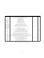
The exhaustive list of all the available parameters within DVA software is quite extensive. We report
in Table 1 the list of all options proper of the deep architecture, while Table 2 contains all options
which can be set for layers.
B
Reading model binary files
The dva executable allows to read those binary files which are produced during the execution of the
program. This is the syntax:
dva -print_bin <double|...|uchar> <bin data file>
where <bin data file> is the input file to be read, which has to be preceded by the type of data
it contains. For example, feature maps S are float, so the command for reading a feature map file is
the following:
dva -print_bin float output/S/layer_0/cat_0/000005/S_0252.bin
10
Parameter
w
h
framerate
frame_min
frame_max
sec_min
sec_max
repeat
num_layers
layeron_secs
layeron_frames
keyframe_secs
keyframe_frames
savemod_secs
savemod_frames
saveout_secs
saveout_frames
sortdata_secs
sortdata_frames
threads
layerpipe
layerpar
mem
rg_threshold
rg_layers
rg_scaler
min_region_size
copf_lambda
copf_rho
copfdesc_rho
copf_stability
copfon_frames
copfon_secs
of_rho
dog_tol
dog_ms_budget
dog_lap_sigma
dog_lap_prune
dog_lapo_prune
dog_max_nodes
scm_kernelparam
scm_bias
scm_lambda
scm_lap_lambda
scm_lap_alpha
scm_maxiter
scm_mingradnorm
scm_cg
scm_run_frames
scm_run_secs
tweak_input
framediff
gw
max_kw
nipals_samples
nipals_frames
scm_exact_ls
scm_lr
scm_lrinc
scm_lrdec
scm_lrmin
scm_lrmax
dog_split
dog_ask_hits
dog_ask_maxfun
dog_ask_frames
dog_ask_secs
dog_rem_hits
dog_rem_frames
dog_rem_secs
palette_dim
Meaning
Width sampling of the video (in pixels)
Height sampling of the video (in pixels)
Frame rate to be adopted
Starting frame
Ending frame
Starting second
Ending second
Number of repetitions of the video
Number of layers
Seconds to be waited to state a layer is complete
Frames to be waited to state a layer is complete
Seconds every which a keyframe is computed
Frames every which a keyframe is computed
Seconds every which the model is saved
Frames every which the model is saved
Seconds every which the output is saved
Frames every which the output is saved
Seconds every which data in Q are sorted
Frames every which data in Q are sorted
Number of threads to be used
Process layers in a parallel pipeline
Process categories in parallel
MB of memory given available to DVA
Threshold for the region growing algorithm: larger values produce larger regions
Number of region-growing layers
Scaler factor to be used within the hierarchical construction of regions
Minimum size of regions, as a percentage of the input
Regularizer for the copf optimization problem
Parameter adjusting the impact of copf on the similarity score, wrt color
Parameter adjusting the impact of copf on the descriptor, wrt color
Threshold for accepting stability on copf frequency matrix
Frames of invariance to be waited before assessing copf stability
Seconds of invariance to be waited before assessing copf stability
Parameter adjusting the impact of optical flow on the similarity score
Radius of the ball surrounding ξ samples, for duplicate matching
Time (in ms) to be spent by DOG for processing a single frame
Sigma of the spatial Laplacian
Threshold for adding an edge in the spatial Laplacian
Threshold for adding an edge in the temporal Laplacian
Maximum number of nodes to be stored within the DOG
Kernel parameter within the rbf kernel in SCM
Bias in SCM
Regularization parameter in SCM
Regularization parameter for the spatial and temporal Laplacian terms in SCM
Balancing parameter between temporal (0) and spatial (1) Laplacian terms in SCM
Max number of SCM iterations per frame
Minimum gradient norm to stop SCM optimization
Whether to use conjugate gradient in SCM
Number of frames every which run SCM
Number of seconds every which run SCM
Prepare input to the first layer by using greyscale levels
Threshold to be used to state whether two consecutive frames are different
Gaussian approximation (2 or 3 in 3µσ)
Maximum width (horizontal) of a not-approximated (spatial) Gaussian kernel
Samples to be used by nipals to extract principal components
Number of frames for the duration of the nipals algorithm
Whether to use exact line search in SCM
Starting learning rate for approximate line search
Learning rate percentage increment for approximate line search
Learning rate percentage decrement for approximate line search
Minimum learning rate for approximate line search
Maximum learning rate for approximate line search
Number of splits into which divide DOG nodes (to speed up computation)
Threshold on DOG hits for asking a supervision: it is a percentage of the total number of nodes
Minimum number of supervisions per function to avoid request
Frames to be waited before asking a supervision (on DVA initiative)
Seconds to be waited before asking a supervision (on DVA initiative)
Threshold on DOG hits for removing a node: it is a percentage of the total number of nodes
Frames to be waited before removing a node in the DOG
Seconds to be waited before removing a node in the DOG
Number of colors in the palette (should be a cube of an integer number)
Range
[0,1]
[0,1]
[0,1]
[0,1]
[0,1]
0/1
{2,3}
–
0/1
{1,8,27,64,125}
Default
-1
-1
-1
-1
-1
-1
-1
1
2
-1
200
-1
200
-1
5
-1
1
60
-1
1
0
0
512
0.01
3
5.0
0.001
0.5
0.1
0.5
1e-3
10
-1
0.001
0.2
-1
0.4
0.9
0.01
3000
0.4
-1
1e-3
1e-4
0.5
50
1e-6
1
1
-1
gray
0.005
3
21
123
200
1
0.01
1.2
0.5
1e-20
1e+5
-1
0.05
5
-1
60
0.01
-1
60
-1
Table 1: Summary of Deep Networks parameters. The bottom part of the table contains the
parameters which it is very unlikely that the user will need to change.
11
Parameter
c
ct
d
di
mu_min
mu_max
blur_secs
blur_frames
sigma_min
sigma_max
sigma_gridsize
mut_min
mut_max
blurt_secs
blurt_frames
sigmat_min
sigmat_max
sigmat_gridsize
angle1_gridsize
angle2_gridsize
angle2_max
angle3_delta
xk_gridsize
xkt_gridsize
lambda
eta
lr
lrinc
lrdec
m0_min
m0_max
xi_tol
xit_tol
axi_tol
axit_tol
const_tol
constt_tol
track_maxdisp
track_minratio
pivots
ms_budget
kernel
kernelparam
maxiter
mingradnorm
qsplit
tsplit
neverending
Meaning
Number of spatial (non-temporal) categories
Number of temporal categories
Number of features (to be split into the categories)
Number of dimensions into which features are projected
Minimum blurring
Maximum blurring
Blurring duration in seconds
Blurring duration in frames
Minimum value for scale
Maximum value for scale
Number of elements in the scale grid
Minimum temporal blurring
Maximum temporal blurring
Temporal blurring duration in seconds
Temporal blurring duration in frames
Minimum value for temporal scale (in seconds)
Maximum value for temporal scale (in seconds)
Number of elements in the temporal scale grid
Number of elements into which the in-plane rotation angle is split
Number of elements into which the tilt angle is split
Width of the receptive field
Width of the temporal receptive field
Regularization parameter for MEE
Balancing parametere for MEE between conditional and global entropies
Initial learning rate for MEE
Percentage increment of learning rate for MEE
Percentage decrement of learning rate for MEE
Minimum initialization value for m parameters in MEE
Maximum initialization value for m parameters in MEE
Threshold for storing ξ elements (the lower, the larger will be Q)
Theshold for storing temporal ξ elements (the lower, the larger will be Qt)
Threshold for storing ξ elements (expressed as an angle)
Threshold for storing temporal ξ elements (expressed as an angle)
Threshold for standard deviation, under which a spatial ξ is considered to be constant
Threshold for standard deviation, under which a temporal ξ is considered to be constant
Maximum displacement between pixels that is tracked by optical flow
Minimum ratio between dot-products of pixel-to-field association during optical flow tracking
Number of pivots to be used for spherical nearest neighbor
Time (in ms) to be spent for processing a single frame
Kernel function for MEE
Kernel parameter for MEE (g for rbf, d for poly)
Maximum number of iterations per frame for MEE
Minimum gradient norm to stop gradient descent in MEE
Number of splits for Q set
Number of splits for transformations set
If set to 1, new ξ elements can always be added
Table 2: Summary of Layer parameters.
12
Range
{ 4, 8, 16, 32 }
{ linear, rbf, poly }
{ 0,1}
Default
1
0
20
3
-1
-1
-1
200
1
4
5
-1
-1
-1
200
-1
2
5
16
3
60
72
9
3
0.001
0.5
0.001
1.2
0.5
-0.1
0.1
0.5
1.0
-1
-1
0.01
0.02
-1
0.9
-1
-1
rbf
1.0
50
1e-6
-1
-1
0