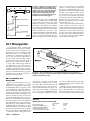
1
Contents 20.1 Transmission Line Basics 20.4.5 Adjusting Antenna Tuners 20.4.6 Myths About SWR 20.1.1 Fundamentals 20.1.2 Matched and Mismatched Lines 20.5 Baluns and Transmission-Line Transformers 20.1.3 Reflection Coefficient and SWR 20.5.1 Quarter-wave Baluns 20.1.4 Losses in Transmission Lines 20.5.2 Transmission Line Transformers 20.2 Choosing a Transmission Line 20.5.3 Coiled-Coax Choke Baluns 20.3 The Transmission Line as Impedance Transformer 20.5.4 Transmitting Ferrite Choke Baluns 20.3.1 Transmission Line Stubs 20.3.2 Transmission Line Stubs as Filters 20.3.3 Project: A Field Day Stub Assembly 20.4 Matching Impedances in the Antenna System 20.4.1 Conjugate Matching 20.4.2 Impedance Matching Networks 20.4.3 Matching Antenna Impedance at the Antenna 20.4.4 Matching the Line to the Transmitter 20.6 Using Transmission Lines in Digital Circuits 20.7 Waveguides 20.7.1 Evolution of a Waveguide 20.7.2 Modes of Waveguide Propagation 20.7.3 Waveguide Dimensions 20.7.4 Coupling to a Waveguide 20.8 Glossary of Transmission Line Terms 20.9 References and Bibliography Chapter 20 Transmission Lines RF power is rarely generated right where it will be used. A transmitter and the antenna it feeds are a good example. The most effective antenna installation is outdoors and clear of ground and energy-absorbing structures. The transmitter, however, is most conveniently installed indoors, where it is out of the weather and is readily accessible. A transmission line is used to convey RF energy from the transmitter to the antenna. A transmission line should transport the RF from the source to its destination with as little loss as possible. This chapter, written by Dean Straw, N6BV, and updated by George Cutsogeorge, W2VJN, explores transmission line theory and applications. Jim Brown, K9YC, contributed updated material on transmitting choke baluns. 20.1 Transmission Line Basics There are three main types of transmission lines used by radio amateurs: coaxial, open-wire and waveguide. The most common type is the coaxial line, usually called coax, shown in various forms in Fig 20.1. Coax is made up of a center conductor, which may be either stranded or solid wire, surrounded by a concentric outer conductor with a dielectric center insulator between the conductors. The outer conductor may be braided shield wire or a metallic sheath. A flexible aluminum foil or a second braided shield is employed in some coax to improve shielding over that obtainable from a standard woven shield braid. If the outer conductor is made of solid aluminum or copper, the coax is referred to as hardline. The second type of transmission line uses parallel conductors, side by side, rather than the concentric ones used in coax. Typical examples of such open-wire lines are 300-Ω TV ribbon line or twin-lead and 450-Ω ladder line (sometimes called window line), also shown in Fig 20.1. Although open-wire lines are enjoying a sort of renaissance in recent years because of their inherently lower losses in simple multiband antenna systems, coaxial cables are far more prevalent because they are much more convenient to use. The third major type of transmission line is the waveguide. While open-wire and coaxial lines are used from power-line frequencies to well into the microwave region, waveguides are used at microwave frequencies only. Waveguides will be covered at the end of this chapter. 20.1.1 Fundamentals In either coaxial or open-wire line, currents flowing in the two conductors travel in opposite directions as shown in Figs 20.1E and 20.1I. If the physical spacing between the two parallel conductors in an open-wire line, S, is small in terms of wavelength, the phase difference between the currents will be very close to 180°. If the two currents also have equal amplitudes, the field generated by each conductor will cancel that generated by the other, and the line will not radiate energy, even if it is many wavelengths long. The equality of amplitude and 180° phase difference of the currents in each conductor in an open-wire line determine the degree of radiation cancellation. If the currents are for some reason unequal, or if the phase difference is not 180°, the line will radiate energy. How such imbalances occur and to what degree they can cause problems will be covered in more detail later. In contrast to an open-wire line, the outer conductor in a coaxial line acts as a shield, confining RF energy within the line as shown in Fig 20.1E. Because of skin effect (see the RF Techniques chapter), current flowing in the outer conductor of a coax does so on the inner surface of the outer conductor. The fields generated by the currents flowing on the outer surface of the inner conductor and on the inner surface of the outer conductor cancel each other out, just as they do in open-wire line. VELOCITY FACTOR In free space, electrical waves travel at the speed of light, or 299,792,458 meters per second. Converting to feet per second yields 983,569,082. The length of a wave in space may be related to frequency as wavelength = λ = velocity/frequency. Thus, the wavelength of a Transmission Lines 20.1 Fig 20.1 — Common types of transmission lines used by amateurs. Coaxial cable, or “coax,” has a center conductor surrounded by insulation. The second conductor, called the shield, cover the insulation and is, in turn, covered by the plastic outer jacket. Various types are shown at A, B, C and D. The currents in coaxial cable flow on the outside of the center conductor and the inside of the outer shield (E). Open-wire line (F, G and H) has two parallel conductors separated by insulation. In open-wire line, the current flows in opposite directions on each wire (I). 1 Hz signal is 983,569,082 ft. Changing to a more useful expression gives: λ= 983.6 f (1) where λ = wavelength, in ft f = frequency in MHz. Thus, at 14 MHz the wavelength is 70.25 ft. Wavelength (λ) may also be expressed in electrical degrees. A full wavelength is 360°, 1 ⁄2 λ is 180°, 1⁄4 λ is 90°, and so forth. Waves travel slower than the speed of light in any medium denser than a vacuum or free space. A transmission line may have an insu20.2 Chapter 20 lator which slows the wave travel down. The actual velocity of the wave is a function of the dielectric characteristic of that insulator. We can express the variation of velocity as the velocity factor for that particular type of dielectric — the fraction of the wave’s velocity of propagation in the transmission line compared to that in free space. The velocity factor is related to the dielectric constant of the material in use. VF = 1 ε where VF = velocity factor ε = dielectric constant. (2) So the wavelength in a real transmission line becomes: 983.6 VF (3) f As an example, many coax cables use polyethylene dielectric over the center conductor as the insulation. The dielectric constant for polyethylene is 2.3, so the VF is 0.66. Thus, wavelength in the cable is about two-thirds as long as a free-space wavelength. The VF and other characteristics of many types of lines, both coax and twin lead, are shown in the table “Nominal Characteristics of Commonly used Transmission Lines” in the Component Data and References chapter. λ= There are differences in VF from batch to batch of transmission line because there are some variations in dielectric constant during the manufacturing processes. When high accuracy is required, it is best to actually measure VF by using an antenna analyzer to measure the resonant frequency of a length of cable. (The antenna analyzer’s user manual will describe the procedure.) Fig 20.2 — Equivalent of an infinitely long lossless transmission line using lumped circuit constants. CHARACTERISTIC IMPEDANCE A perfectly lossless transmission line may be represented by a whole series of small inductors and capacitors connected in an infinitely long line, as shown in Fig 20.2. (We first consider this special case because we need not consider how the line is terminated at its end, since there is no end.) Each inductor in Fig 20.2 represents the inductance of a very short section of one wire and each capacitor represents the capacitance between two such short sections. The inductance and capacitance values per unit of line depend on the size of the conductors and the spacing between them. Each series inductor acts to limit the rate at which current can charge the following shunt capacitor, and in so doing establishes a very important property of a transmission line: its surge impedance, more commonly known as its characteristic impedance. This is usually abbreviated as Z0, d, a or b, as long as they are the same units. A line with closely spaced, large conductors will have a low characteristic impedance, while one with widely spaced, small conductors will have a relatively high characteristic impedance. Practical open-wire lines exhibit characteristic impedances ranging from about 200 to 800 Ω, while coax cables have Z0 values between 25 to 100 Ω. Except in special instances, coax used in amateur radio has an impedance of 50 or 75 Ω. All practical transmission lines exhibit some power loss. These losses occur in the resistance that is inherent in the conductors that make up the line, and from leakage currents flowing in the dielectric material between the conductors. We’ll next consider what happens when a real transmission line, which is not infinitely long, is terminated in an actual load impedance, such as an antenna. L C where L and C are the inductance and capacitance per unit length of line. The characteristic impedance of an airinsulated parallel-conductor line, neglecting the effect of the insulating spacers, is given by Z0 ≈ Z0 = 120 ε cosh −1 S d (4) where Z0 = characteristic impedance S = center to center distance between the conductors d = diameter of conductors in the same units as S When S >> d, the approximation Z0 = 276 log10 (2S/d) may be used but for S < 2d gives values that are significantly higher than the correct value, such as is often the case when wires are twisted together to form a transmission line for impedance transformers. The characteristic impedance of an airinsulated coaxial line is given by b Z 0 = 138 log10 a (5) where Z0 = characteristic impedance b = inside diameter of outer conductors a = outside diameter of inner conductor (in same units as b). It does not matter what units are used for S, 20.1.2 Matched and Mismatched Lines Real transmission lines do not extend to infinity, but have a definite length. In use they are connected to, or terminate in, a load (such as an antenna), as illustrated in Fig 20.3A. If the load is a pure resistance whose value equals the characteristic impedance of the line, the line is said to be matched. To current traveling along the line, such a load at the end of the line acts as though it were still more transmission line of the same characteristic impedance. In a matched transmission line, energy travels outward along the line from the source until it reaches the load, where it is completely absorbed (or radiated if the load is an antenna). MISMATCHED LINES Assume now that the line in Fig 20.3B is terminated in an impedance Za which is not equal to Z0 of the transmission line. The line is now a mismatched line. RF energy reaching the end of a mismatched line will not be fully absorbed by the load impedance. Instead, part of the energy will be reflected back toward the source. The amount of reflected versus absorbed energy depends on the degree of mismatch between the characteristic impedance of the line and the load impedance connected to its end. The reason why energy is reflected at a discontinuity of impedance on a transmission line can best be understood by examining Fig 20.3 — At A the coaxial transmission line is terminated with resistance equal to its Z0. All power is absorbed in the load. At B, coaxial line is shown terminated in an impedance consisting of a resistance and a capacitive reactance. This is a mismatched line, and a reflected wave will be returned back down the line toward the generator. The reflected wave adds to the forward wave, producing a standing wave on the line. The amount of reflection depends on the difference between the load impedance and the characteristic impedance of the transmission line. some limiting cases. First, consider the rather extreme case where the line is shorted at its end. Energy flowing to the load will encounter the short at the end, and the voltage at that point will go to zero, while the current will rise to a maximum. Since the current can’t develop any power in a dead short, the energy will all be reflected back toward the source generator. If the short at the end of the line is replaced with an open circuit, the opposite will happen. Here the voltage will rise to maximum, and the current will by definition go to zero. The phase will reverse, and all energy will be reflected back towards the source. By the way, if this sounds to you like what happens at the end of a half-wavelength dipole antenna, you are quite correct. However, in the case of an antenna, energy traveling along the antenna is lost by radiation on purpose, whereas a good transmission line will lose little energy to radiation because of field cancellation between the two conductors. For load impedances falling between Transmission Lines 20.3 the extremes of short- and open-circuit, the phase and amplitude of the reflected wave will vary. The amount of energy reflected and the amount of energy absorbed in the load will depend on the difference between the characteristic impedance of the line and the impedance of the load at its end. What actually happens to the energy reflected back down the line? This energy will encounter another impedance discontinuity, this time at the generator. Reflected energy flows back and forth between the mismatches at the source and load. After a few such journeys, the reflected wave diminishes to nothing, partly as a result of finite losses in the line, but mainly because of absorption at the load. In fact, if the load is an antenna, such absorption at the load is desirable, since the energy is actually radiated by the antenna. If a continuous RF voltage is applied to the terminals of a transmission line, the voltage at any point along the line will consist of a vector sum of voltages, the composite of waves traveling toward the load and waves traveling back toward the source generator. The sum of the waves traveling toward the load is called the forward or incident wave, while the sum of the waves traveling toward the generator is called the reflected wave. 20.1.3 Reflection Coefficient and SWR In a mismatched transmission line, the ratio of the voltage in the reflected wave at any one point on the line to the voltage in the forward wave at that same point is defined as the voltage reflection coefficient. This has the same value as the current reflection coefficient. The reflection coefficient is a complex quantity (that is, having both amplitude and phase) and is generally designated by the Greek letter ρ (rho), or sometimes in the professional literature as Γ (Gamma). The relationship between Rl (the load resistance), Xl (the load reactance), Z0 (the line characteristic impedance, whose real part is R0 and whose reactive part is X0) and the complex reflection coefficient ρ is ρ= Z l − Z 0 (R l ± jX l ) − (R 0 ± jX 0 ) (6) = Z l + Z 0 (R l ± jX l ) + (R 0 ± jX 0 ) For most transmission lines the characteristic impedance Z0 is almost completely resistive, meaning that Z0 = R0 and X0 ≅ 0. The magnitude of the complex reflection coefficient in equation 6 then simplifies to: tive reactance of –90 Ω, the magnitude of the reflection coefficient is ρ= (120 − 50)2 + ( −90)2 (120 + 50)2 + ( −90)2 = 0.593 Note that if Rl in equation 6 is equal to R0 and Xl is 0, the reflection coefficient, ρ, is 0. This represents a matched condition, where all the energy in the incident wave is transferred to the load. On the other hand, if Rl is 0, meaning that the load is a short circuit and has no real resistive part, the reflection coefficient is 1.0, regardless of the value of R0. This means that all the forward power is reflected since the load is completely reactive. The concept of reflection is often shown in terms of the return loss (RL), which is given in dB and is equal to 20 times the log of the reciprocal of the reflection coefficient. P RL(dB) = −10 log r = −20 log(ρ) P f (8) 1+ ρ 1− ρ (9A) SWR − 1 SWR + 1 (9B) and ρ= (R l − R 0 )2 + X l 2 (R l + R 0 )2 + X l 2 (7) example, if the characteristic impedFor ance of a coaxial line is 50 Ω and the load impedance is 120 Ω in series with a capaci20.4 Chapter 20 ρ= Pr ρ= Pf in equations 8 and 9 are The definitions valid for any line length and for lines which are lossy, not just lossless lines longer than (10A) and 1+ SWR = In the example above, the return loss is 20 log (1/0.593) = 4.5 dB. If there are no reflections from the load, the voltage distribution along the line is constant or flat. A line operating under these conditions is called either a matched or a flat line. If reflections do exist, a voltage standing-wave pattern will result from the interaction of the forward and reflected waves along the line. For a lossless transmission line at least 1⁄4-λ long, the ratio of the maximum peak voltage anywhere on the line to the minimum value anywhere along the line is defined as the voltage standing-wave ratio, or VSWR. (The line must be 1⁄4 λ or longer for the true maximum and minimum to be created.) Reflections from the load also produce a standing-wave pattern of currents flowing in the line. The ratio of maximum to minimum current, or ISWR, is identical to the VSWR in a given line. In amateur literature, the abbreviation SWR is commonly used for standing-wave ratio, as the results are identical when taken from proper measurements of either current or voltage. Since SWR is a ratio of maximum to minimum, it can never be less than one-toone. In other words, a perfectly flat line has an SWR of 1:1. The SWR is related to the magnitude of the complex reflection coefficient and vice versa by SWR = ⁄4 λ at the frequency in use. Very often the load impedance is not exactly known, since an antenna usually terminates a transmission line, and the antenna impedance may be influenced by a host of factors, including its height above ground, end effects from insulators, and the effects of nearby conductors. We may also express the reflection coefficient in terms of forward and reflected power, quantities which can be easily measured using a directional RF wattmeter. The reflection coefficient and SWR may be computed as 1 Pr Pf P 1− r Pf (10B) where Pr = power in the reflected wave Pf = power in the forward wave. If a line is not matched (SWR > 1:1) the difference between the forward and reflected powers measured at any point on the line is the net power going toward the load from that point. The forward power measured with a directional wattmeter (often referred to as a reflected power meter or reflectometer) on a mismatched line will thus always appear greater than the forward power measured on a flat line with a 1:1 SWR. The software program TLW, written by Dean Straw, N6BV, and included on the ARRL Antenna Book CD solves these complex equations. This should come as a big relief for most radio amateurs. The characteristics of many common types of transmission lines are included in the software so that real antenna matching problems may be easily solved. Detailed instructions on using the program are included with it. The various examples in this chapter have been solved with TLW. Equation 6 is also solved in a normalized form with a graphical method called the Smith Chart. Matching problems can be handled much easier than solving complex arithmetic equations by using this polar chart. More detailed information about using the Smith Chart is included in The ARRL Antenna Book. Many references to Smith Charts and their use may be found on the Web. 20.1.4 Losses in Transmission Lines A real transmission line exhibits a certain amount of loss, caused by the resistance of the conductors used in the line and by dielectric losses in the line’s insulators. The matchedline loss for a particular type and length of transmission line, operated at a particular frequency, is the loss when the line is terminated in a resistance equal to its characteristic impedance. The loss in a line is lowest when it is operated as a matched line. Line losses increase when SWR is greater than 1:1. Each time energy flows from the generator toward the load, or is reflected at the load and travels back toward the generator, a certain amount will be lost along the line. The net effect of standing waves on a transmission line is to increase the average value of current and voltage, compared to the matched-line case. An increase in current raises I2R (ohmic) losses in the conductors, and an increase in RF voltage increases E2/R losses in the dielectric. Line loss rises with frequency, since the conductor resistance is related to skin effect, and also because dielectric losses rise with frequency. Matched-line loss (ML) is stated in decibels per hundred feet at a particular frequency. The matched-line loss per hundred feet versus frequency for a number of common types of lines, both coaxial and open-wire balanced types, is shown graphically and as a table in the Component Data and References chapter. For example, RG-213 coax cable has a matched-line loss of 2.5 dB/100 ft at 100 MHz. Thus, 45 ft of this cable feeding a 50-Ω load at 100 MHz would have a loss of of the line. This does not mean that the load is absorbing any more power. Line loss absorbs power as it travels to the load and again on its way back to the generator, so the difference between the generator output power and the power returning from the load is higher than for a lossless line. Thus, Pr/Pf is smaller than at the load and so is the measured SWR. For example, RG-213 solid-dielectric coax cable exhibits a matched-line loss at 28 MHz of 1.14 dB per 100 ft. A 250-ft length of this cable has a matched-line loss of 1.14 × 250/100 = 2.86 dB. Assume that we measure the SWR at the load as 6:1, the total mismatched line loss from equation 11 is 5.32 dB. The additional loss due to the 6:1 SWR at 28 MHz is 5.32 – 2.86 = 2.46 dB. The SWR at the input of the 250-ft line is only 2.2:1, because line loss has masked the true magnitude of SWR (6:1) at the load end of the line. The losses increase if coax with a larger matched-line loss is used under the same conditions. For example, RG-58A coaxial cable is about one-half the diameter of RG-213, and it has a matched-line loss of 2.81 dB/ 100 ft at 28 MHz. A 250-ft length of RG58A has a total matched-line loss of 7.0 dB. With a 6:1 SWR at the load, the additional loss due to SWR is 3.0 dB, for a total loss of 10.0 dB. The additional cable loss due to the mismatch reduces the SWR measured at the input of the line to 1.33:1. An unsuspecting operator measuring the SWR at his transmitter might well believe that everything is just 2.5 dB fine, when in truth only about 10% of the Matched line loss = × 45 ft transmitter power is getting to the antenna! 100 ft Be suspicious of very low SWR readings for an antenna fed with a long length of coaxial = 1.13dB cable, especially if the SWR remains low If a line is not matched, standing waves across a wide frequency range. Most antennas will cause additional loss beyond the inherent have narrow SWR bandwidths, and the SWR matched-line loss for that line. should change across a band. a 2 On − ρ2the other hand, if expensive 7⁄8-inch Total Mismatched Line Loss (dB) = 10 l og diameter 50-Ω hardline cable is used at − ρ2 the a 281 MHz, matched-line loss is only 0.19 dB/ 100 ft. For 250 ft of this Hardline, the matched a 2 − ρ2 line loss is 0.475 dB, and the additional loss ne Loss (dB) = 10 l og (11) due to a 6:1 SWR is 0.793 dB. Thus, the total 2 loss is 1.27 dB. a 1 − ρ At the upper end of the HF spectrum, when the transmitter and antenna are separated by where a long transmission line, the use of bargain a = 10ML/10 coax may prove to be a very poor cost-saving ML = the line’s matched loss in dB. strategy. Adding a 1500-W linear amplifier (providing 8.7 dB of gain over a 200 W transFor most types of line and for modest values mitter), to offset the loss in RG-58A comof SWR, the additional line loss due to SWR pared to hardline, would cost a great deal is of little concern. As the line’s loss increases more than higher-quality coax. Furthermore, or at higher frequencies, the total line loss (the no transmitting amplifier can boost receiver sum of matched-line loss and additional loss sensitivity — loss in the line has the same due to SWR) can be surprisingly high at high effect as putting an attenuator in front of the values of SWR. receiver. Because of losses in a transmission line, At the lower end of the HF spectrum, say the measured SWR at the input of the line is 3.5 MHz, the amount of loss in common coax lower than the SWR measured at the load end lines is less of a problem for the range of SWR ( ( ) ) Fig 20.4 — Increase in line loss because of standing waves (SWR measured at the load). To determine the total loss in decibels in a line having an SWR greater than 1, first determine the matched-line loss for the particular type of line, length and frequency, on the assumption that the line is perfectly matched. For example, Belden 9913 has a matched-line loss of 0.49 dB/100 ft at 14 MHz. Locate 0.49 dB on the horizontal axis. For an SWR of 5:1, move up to the curve corresponding to this SWR. The increase in loss due to SWR is 0.66 dB beyond the matched line loss. values typical on this band. For example, consider an 80 meter dipole cut for the middle of the band at 3.75 MHz. It exhibits an SWR of about 6:1 at the 3.5 and 4.0 MHz ends of the band. At 3.5 MHz, 250 ft of RG-58A small-diameter coax has an additional loss of 2.1 dB for this SWR, giving a total line loss of 4.0 dB. If larger-diameter RG-213 coax is used instead, the additional loss due to SWR is 1.3 dB, for a total loss of 2.2 dB. This is an acceptable level of loss for most 80-meter operators. The loss situation gets dramatically worse as the frequency increases into the VHF and UHF regions. At 146 MHz, the total loss in 250 ft of RG-58A with a 6:1 SWR at the load is 21.4 dB, 10.1 dB for RG-213A, and 2.7 dB for 7⁄8-inch, 50-Ω hardline. At VHF and UHF, a low SWR is essential to keep line losses low, even for the best coaxial cable. The length of transmission line must be kept as short as practical at these frequencies. The effect of SWR on line loss is shown graphically in Fig 20.4. The horizontal axis is the attenuation, in decibels, of the line when perfectly matched. The vertical axis gives the additional attenuation due to SWR. If long coaxial cable transmission lines are necessary, the matched loss of the coax used should be kept as low as possible, meaning that the highest-quality, largest-diameter cable should be used. Transmission Lines 20.5 20.2 Choosing a Transmission Line It is no accident that coaxial cable has become as popular as it has since it was first widely used during WWII. Coax is mechanically much easier to use than open-wire line. Because of the excellent shielding afforded by its outer shield, coax can be run up a metal tower leg, taped together with numerous other cables, with virtually no interaction or crosstalk between the cables. At the top of a tower, coax can be used with a rotatable Yagi or quad antenna without worrying about shorting or twisting the conductors, which might happen with an open-wire line. Class 2 PVC (P2) noncontaminating outer jackets are designed for long-life outdoor installations. Class 1 PVC (P1) outer jackets are not recommended for outdoor installations. (See the table of coaxial cables in the Component Data and References chapter.) Coax can be buried underground, especially if it is run in plastic piping (with suitable drain holes) so that ground water and soil chemicals cannot easily deteriorate the cable. A cable with an outer jacket of polyethylene (PE) rather than polyvinyl chloride (PVC) is recommended for direct-bury installations. Open-wire line must be carefully spaced away from nearby conductors, by at least several times the spacing between its conductors, to minimize possible electrical imbalances between the two parallel conductors. Such imbalances lead to line radiation and extra losses. One popular type of open-wire line is called ladder line because the insulators used to separate the two parallel, uninsulated conductors of the line resemble the steps of a ladder. Long lengths of ladder line can twist together in the wind and short together if not properly supported. MULTIBAND OPERATION WITH OPEN WIRE LINE Despite the mechanical difficulties associated with open-wire line, there are some compelling reasons for its use, especially in simple multiband antenna systems. Every antenna system, no matter what its physical form, exhibits a definite value of impedance at the point where the transmission line is connected. Although the input impedance of an antenna system is seldom known exactly, it is often possible to make a close estimate of its value with computer modeling software. As an example, Table 20.1 lists the computed characteristics versus frequency for a multiband, 100-ft long center-fed dipole, placed 50 ft above average ground. These values were computed using EZNEC-3. A nonresonant 100-ft length was chosen as an illustration of a practical size that many radio amateurs could fit into their backyards, although nothing in particular recommends this antenna over other forms. It is merely used as an example. Examine Table 20.1 carefully in the following discussion. Columns three and four show the SWR on a 50-Ω RG-213 coaxial transmission line directly connected to the antenna, followed by the total loss in 100 ft of this cable. The impedance for this nonresonant, 100-ft long antenna varies over a very wide range for the nine operating frequencies. The SWR on a 50-Ω coax connected directly to this antenna would be extremely high on some frequencies, particularly at 1.8 MHz, where the antenna is highly capacitive because it is very short of resonance. The loss in 100 ft of RG-213 at 1.8 MHz is a staggering 26 dB. Contrast this to the loss in 100 ft of 450-Ω open-wire line. Here, the loss at 1.8 MHz is 8.8 dB. While 8.8 dB of loss is not particularly desirable, it is about 17 dB better than the coax! Note that the RG-213 coax exhibits a good deal of loss on almost all the bands due to mismatch. Only on 14 MHz does the loss drop down to 0.9 dB, where the antenna is just past 3⁄2-λ resonance. From 3.8 to 28.4 MHz the open-wire line has a maximum loss of only 0.6 dB. Columns six and seven in Table 20.1 list the maximum RMS voltage for 1500 W of RF power on the 50-Ω coax and on the 450-Ω open-wire line. The maximum RMS voltage for 1500 W on the open-wire line is extremely high, at 10,950 V at 1.8 MHz. The voltage for a 100-W transmitter would be reduced by a ratio of 1500 = 3.87 :1 100 This is 2829 V, still high enough to cause arcing in many antenna tuners, although it only occurs at specific points that are multiples of 1⁄2 λ from the load. In practice, the lower voltages present along the transmission line are within the operating range of most tuners although you should remain aware that high voltages may be present along the line at some points. Table 20.1 Modeled Data for a 100-ft Flat-Top Antenna Freq (MHz) 1.8 3.8 7.1 10.1 14.1 18.1 21.1 24.9 28.4 Antenna Impedance (Ω) 4.18 –j 1590 37.5 –j 354 447 +j 956 2010 –j 2970 87.6 –j 156 1800 +j 1470 461 –j 1250 155 +j 150 2590 +j 772 Input VSWR RG-213 Coax 33.7 16.7 12.3 12.1 1.6 7.7 4.6 3.6 6.7 Loss of 100 ft RG-213 Coax (dB) 26.0 5.7 5.9 10.1 0.9 6.8 3.2 2.6 9.4 Loss of 100 ft 450-Ω Line (dB) 8.8 0.5 0.2 0.6 0.3 0.3 0.1 0.2 0.5 Max Voltage RG-213 Coax at 1500 W 1507 1177 985 967 344 753 585 516 703 Max Voltage 450-Ω Line at 1500 W 10950 3231 2001 2911 1632 1600 828 1328 1950 Notes 1) Antenna is a 100 ft long, 50 ft high, center-fed dipole over average ground, using coaxial (RG-213) or open-wire transmission lines. Each transmission line is 100 ft long. 2) Antenna impedance computed using EZNEC-3 computer program using 499 segments and with the Real Ground model. 3) Note the extremely reactive impedance levels at many frequencies, but especially at 1.8 MHz. If this antenna is fed directly with RG-213 coax, the losses are unacceptably large on 160 meters, and undesirably high on most other bands also. 4) The RF voltage at 1.8 MHz for high-power operation with open-wire line is extremely high also, and would probably result in arcing either on the line itself, or more likely in the antenna tuner. 20.6 Chapter 20 In general, such a nonresonant antenna is a proven, practical multiband radiator when fed with 450-Ω open-wire ladder line connected to an antenna tuner. A longer antenna would be preferable for more efficient 160 meter operation, even with open-wire line. The tuner and the line itself must be capable of handling the high RF voltages and currents involved for high-power operation. On the other hand, if such a multiband antenna is fed directly with coaxial cable, the losses on most frequencies are prohibitive. Coax is most suitable for antennas whose resonant feed-point impedances are close to the characteristic impedance of the feed line. 20.3 The Transmission Line as Impedance Transformer If the complex mechanics of reflections, SWR and line losses are put aside momentarily, a transmission line can very simply be considered as an impedance transformer. A certain value of load impedance, consisting of a resistance and reactance, at the end of the line is transformed into another value of impedance at the input of the line. The amount of transformation is determined by the electrical length of the line, its characteristic impedance, and by the losses inherent in the line. The input impedance of a real, lossy transmission line is computed using the following equation Z in = Z 0 × Z L cosh ( η) + Z 0 sinh ( η) Z L sinh ( η) + Z 0 cosh ( η) (12) where Zin = complex impedance at input of line = Rin ± j Xin ZL = complex load impedance at end of line = Rl ± j Xl Z0 = characteristic impedance of line = R0 ± j X0 η = complex loss coefficient = α + j β α = matched line loss attenuation constant, in nepers/unit length (1 neper = 8.688 dB, so multiply line loss in dB per unit length by 8.688) β = phase constant of line in radians/unit length (multiply electrical length in degrees by 2π radians/360 degrees) = electrical length of line in same units of length as used for α. Solving this equation manually is tedious, since it incorporates hyperbolic cosines and sines of the complex loss coefficient, but it may be solved using a traditional paper Smith Chart or a computer program. The ARRL Antenna Book has a chapter detailing the use of the Smith Chart. TLW software performs this transformation, but without Smith Chart graphics. 20.3.1 Transmission Line Stubs The impedance-transformation properties of a transmission line are useful in a number of applications. If the terminating resistance is zero (that is, a short) at the end of a lowloss transmission line which is less than 1⁄4-λ long, the input impedance consists of a reactance, which is given by a simplification of equation 12. Fig 20.5 — Method of attaching a stub to a feed line. X in ≅ Z 0 tan (13) If the line termination is an open circuit, the input reactance is given by X in = Z 0 cot (14) The input of a short (less than 1⁄4-λ) length of line with a short circuit as a terminating load appears as an inductance, while an opencircuited line appears as a capacitance. This is a useful property of a transmission line, since it can be used as a low-loss inductor or capacitor in matching networks. Such lines are often referred to as stubs. A line that is electrically 1⁄4-λ long is a special kind of a stub. When a 1⁄4-λ line is short circuited at its load end, it presents an open circuit at its input. Conversely, a 1⁄4-λ line with an open circuit at its load end presents a short circuit at its input. Such a line inverts the impedance of a short or an open circuit at the frequency for which the line is 1⁄4-λ long. This is also true for frequencies that are odd multiples of the 1⁄4-λ frequency. However, for frequencies where the length of the line is 1 ⁄2-λ, or integer multiples thereof, the line will duplicate the termination at its end. 20.3.2 Transmission Line Stubs as Filters The impedance transformation properties of stubs can be put to use as filters. For example, if a shorted line is cut to be 1⁄4-λ long at 7.1 MHz, the impedance looking into the input of the cable will be an open circuit. The line will have no effect if placed in parallel with a transmitter’s output terminals. However, at twice the fundamental frequency, 14.2 MHz, that same line is now 1⁄2-λ, and the line looks like a short circuit. The line, often dubbed a quarter-wave stub in this application, will act as a trap for not only the second harmonic, but also for higher even-order harmonics, such as the fourth or sixth harmonics. This filtering action is extremely useful in multitransmitter situations, such as Field Day, emergency operations centers, portable communications facilities and multioperator contest stations. Transmission line stubs can operate at high power where lumped-constant filters would be expensive. Using stub filters reduces noise, harmonics and strong fundamental signals from the closely spaced antennas that cause overload and interference to receivers. Quarter-wave stubs made of good-quality coax, such as RG-213, offer a convenient way to lower transmitter harmonic levels. Despite the fact that the exact amount of harmonic attenuation depends on the impedance (often unknown) into which they are working at the harmonic frequency, a quarter-wave stub will typically yield 20 to 25 dB of attenuation of the second harmonic when placed directly at the output of a transmitter feeding common amateur antennas. Because different manufacturing runs of coax will have slightly different velocity factors, a quarter-wave stub is usually cut a little longer than calculated, and then carefully pruned by snipping off short pieces, while using an antenna analyzer to monitor the response at the fundamental frequency. Because the end of the coax is an open circuit while pieces are being snipped away, the input of a 1 ⁄4-λ line will show a short circuit exactly at the fundamental frequency. Once the coax has been pruned to frequency, a short jumper is soldered across the end, and the response at the second harmonic frequency is measured. Fig 20.5 shows how to connect a shorted stub to a transmission line and Fig 20.6 shows a typical frequency response. The shorted quarter-wave stub shows low Transmission Lines 20.7 loss at 7 MHz and at 21 MHz where it is ⁄4 -λ long. It nulls 14 and 28 MHz. This is useful for reducing the even harmonics of a 7 MHz transmitter. It can be used for a 21 MHz transmitter as well, and will reduce any spurious emissions such as phase noise and wideband noise which might cause interference to receivers operating on 14 or 28 MHz. The open-circuited quarter-wave stub has a low impedance at the fundamental frequency, so it must be used at two times the frequency for which it is cut. For example, a quarter-wave open stub cut for 3.5 MHz will present a high impedance at 7 MHz where it is 1⁄2-λ long. It will present a high impedance at those frequencies where it is a multiple of 1 ⁄2-λ, or 7, 14 and 28 MHz. It would be connected in the same manner as Fig 20.5 shows, and the frequency plot is shown in Fig 20.7. This open stub can protect a receiver operating on 7, 14, 21 or 28 MHz from interference by a 3.5 MHz transmitter. It also has nulls at 10.5, 17.5 and 24.5 MHz — the 3rd, 5th and 7th harmonics. The length of a quarter-wave stub may be calculated as follows: 3 Le = VF × 983.6 4f (15) where Le = length in ft VF = propagation constant for the coax in use f = frequency in MHz. For the special case of RG-213 (and any similar cable with VF = 0.66), equation 15 can be simplified to: Le = 163.5 f (16) where Le = length in ft f = frequency in MHz. Table 20.2 solves this equation for the major contesting bands where stubs are often used. The third column shows how much of the stub to cut off if the desired frequency is 100 kHz higher in frequency. For example: To cut a stub for 14.250 MHz, reduce the overall length shown by 2.5 × 1 inches, or 2.5 inches. There is some variation in dielectric constant of coaxial cable from batch to batch or manufacturer to manufacturer, so it is always best to measure the stub’s fundamental resonance before proceeding. CONNECTING STUBS Stubs are usually connected in the antenna feed line close to the transmitter. They may also be connected on the antenna side of a switch used to select different antennas. Some small differences in the null depth may occur for different positions. To connect a stub to the transmission line it is necessary to insert a coaxial T (as shown in 20.8 Chapter 20 Fig 20.6 — Frequency response with a shorted stub. Fig 20.7 — Frequency response with an open stub. Table 20.2 Quarter-Wave Stub Lengths for the HF Contesting Bands Freq Length (Le)* (MHz) 1.8 90 ft, 10 in 3.5 46 ft, 9 in 7.0 23 ft, 4 in 14.0 11 ft, 8 in 21.0 7 ft, 9 in 28.0 5 ft, 10 in Cut off per 100 kHz 573⁄8 in 151⁄2 in 4 in 1 in 7 ⁄16 in 1 ⁄4 in *Lengths shown are for RG-213 and any similar cable, assuming a 0.66 velocity factor (Le = 163.5/f). See text for other cables. Fig 20.5). If a female-male-female T is used, the male can connect directly to the transmitter while the antenna line and the stub connect to the two females. It should be noted that the T inserts a small additional length in series with the stub that lowers the resonant frequency. The additional length for an Amphenol UHF T is about 3⁄8 inch. This length is negligible at 1.8 and 3.5 MHz, but on the higher bands it should not be ignored. MEASURING STUBS WITH ONE-PORT METERS Many of the common measuring instruments used by amateurs are one-port devices, meaning they have one connector at which the measurement — typically VSWR — is made. Probably the most popular instrument for this type of work is the antenna analyzer, available from a number of manufacturers. To test a stub using an antenna analyzer, connect the stub to the meter by itself and tune the meter for a minimum impedance value, ignoring the VSWR setting. It is almost impossible to get an accurate reading on the higher HF bands, particularly with open stubs. For example, when a quarter-wave open stub cut for 20 meters was nulled on an MFJ259 SWR analyzer, the frequency measured 14.650 MHz, with a very broad null. A recheck with a professional-quality network analyzer measured 14.018 MHz. (Resolution on the network analyzer is about ±5 kHz.) Running the same test on a quarter-wave shorted stub gave a measurement of 28.320 MHz on the MFJ-259 and 28.398 MHz on the network analyzer. (These inaccuracies are typical of amateur instrumentation and are meant to illustrate the difficulties of using inexpensive instruments for sensitive measurements.) Other one-port instruments that measure phase can be used to get a more accurate reading. The additional length added by the required T must be accounted for. If the measurement is made without the T and then with the T, the average value will be close to correct. MEASURING STUBS WITH TWOPORT INSTRUMENTS A two-port measurement is made with a signal generator and a separate detector. A T connector is attached to the generator with the stub connected to one side. The other side is connected to a cable of any length that goes to the detector. The detector should present a 50-Ω load to the cable. This is how a network analyzer is configured, and it is similar to how the stub is connected in actual use. If the generator is accurately calibrated, the measurement can be very good. There are a number of ways to do this without buying an expensive piece of lab equipment. An antenna analyzer can be used as the signal generator. Measurements will be quite accurate if the detector has 30 to 40 dB dynamic range. Two setups were tested by the author for accuracy. The first used a digital voltmeter (DVM) with a diode detector. (A germanium diode must be used for the best dynamic range.) Tests on open and shorted stubs at 14 MHz returned readings within 20 kHz of the network analyzer. Another test was run using an oscilloscope as the detector with a 50-Ω load on the input. This test produced results that were essentially the same as the network analyzer. A noise generator can be used in combination with a receiver as the detector. (An inexpensive noise generator kit is available from Elecraft, www.elecraft.com.) Set the receiver for 2-3 kHz bandwidth and turn off the AGC. An ac voltmeter connected to the audio output of the receiver will serve as a null detector. The noise level into the receiver without the stub connected should be just at or below the limiting level. With the stub connected, the noise level in the null should drop by 25 or 30 dB. Connect the UHF T to the noise generator using any necessary adapters. Connect the stub to one side of the T and connect the receiver to the other side with a short cable. Tune the receiver around the expected null frequency. After locating the null, snip off pieces of cable until the null moves to the desired frequency. Accuracy with this method is within 20 or 30 kHz of the network analyzer readings on 14 MHz stubs. STUB COMBINATIONS A single stub will give 20 to 30 dB attenuation in the null. If more attenuation is needed, two or more similar stubs can be combined. Best results will be obtained if a short coupling cable is used to connect the two stubs rather than connecting them directly in parallel. The stubs may be cut to the same frequency for maximum attenuation, or to two slightly different frequencies such as the CW and SSB frequencies in one band. Open and shorted stubs can be combined together to attenuate higher harmonics as well as lower frequency bands. An interesting combination is the parallel connection of two 1⁄8-λ stubs, one open and the other shorted. The shorted stub will act as an inductor and the open stub as a capacitor. Their reactance will be equal and opposite, forming a resonant circuit. The null depth with this arrangement will be a bit better than a single quarter-wave shorted stub. This presents some possibilities when combinations of stubs are used in a band switching system. Table 20.3 Stub Selector Operation See Fig 20.8 for circuit details. Relay K1 Relay K2 Position Position Open Open Energized Energized Energized Open Open Energized Bands Passed (meters) All 80 40, 15 20, 10 Bands Nulled (meters) None 40, 20, 15, 10 20, 10 40, 15 20.3.3 Project: A Field Day Stub Assembly Fig 20.8 — Schematic of the Field Day stub switching relay control box. Table 20.3 shows which relays should be closed for the desired operating band. Fig 20.8 shows a simple stub arrangement that can be useful in a two-transmitter Field Day station. The stubs reduce out-of-band noise produced by the transmitters that would cause interference to the other stations — a common Field Day problem where the stations are quite close together. This noise can not be filtered out at the receiver and must be removed at the transmitter. One stub assembly would be connected to each transmitter output and manually switched for the appropriate band. Two stubs are connected as shown. The two-relay selector box can be switched in four ways. Stub 1 is a shorted quarter-wave 40-meter stub. Stub 2 is an open quarterwave 40-meter stub. Operation is as shown in Table 20.3. The stubs must be cut and tuned while connected to the selector relays. RG-213 may be used for any amateur power level and will provide 25 to 30 dB reduction in the nulls. For power levels under 500 W or so, RG-8X may be used. It will provide a few dB less reduction in the nulls because of its slightly higher loss than RG-213. 20.4 Matching Impedances in the Antenna System Only in a few special cases is the antenna impedance the exact value needed to match a practical transmission line. In all other cases, it is necessary either to operate with a mismatch and accept the SWR that results, or else to bring about a match between the line and the antenna. When transmission lines are used with a transmitter, the most common load is an antenna. When a transmission line is connected between an antenna and a receiver, the receiver input circuit is the load, not the antenna, because the power taken from a passing wave is delivered to the receiver. Whatever the application, the conditions existing at the load, and only the load, determine the reflection coefficient, and hence the SWR, on the line. If the load is purely resistive and equal to the characteristic impedance of the line, there will be no standing waves. If the load is not purely resistive, or is not equal to the line Z0, there will be standing waves. No adjustments can be made at the input end of the line to change the SWR at the load. Neither is the SWR affected by changing the line length, except as previously described when the SWR at the input of a lossy line is masked by the attenuation of the line. 20.4.1 Conjugate Matching Technical literature sometimes uses the term conjugate match to describe the condition where the impedance seen looking toward the load from any point on the line is the complex conjugate of the impedance seen looking toward the source. This means that the resistive and reactive magnitudes of the impedances are the same, but that the reactances have opposite signs. For example, the complex conjugate of 20 + j 75 is 20 – j 75. The complex conjugate of a purely resistive impedance, such as 50 + j 0 Ω, is the same impedance, 50 + j 0 Ω. A conjugate match is necessary to achieve the maximum power gain possible from most signal sources. For example, if 50 ft of RG-213 is terminated in a 72 – j 34 Ω antenna impedance, the transmission line transforms the impedance to 35.9 – j 21.9 Ω at its input. (The TLW program is used to calculate the impedance at the line input.) To create a conjugate match at the line input, a matching network would have to present an impedance of 35.9 + j 21.9 Ω. The system would then become resonant, since the ± j 21.9 Ω react ances would cancel, leaving 35.9 + j 0 Ω. Transmission Lines 20.9 A conjugate match is not the same as transforming one impedance to another, such as from 35.9 – j 0 Ω to 50 + j 0 Ω. An additional impedance transformation network would be required for that step. Conjugate matching is often used for smallsignal amplifiers, such preamps at VHF and above, to obtain the best power gain. The situation with high-power amplifiers is complex and there is considerable discussion as to whether conjugate matching delivers the highest efficiency, gain and power output. Nevertheless, conjugate matching is the model most often applied to impedance matching in antenna systems. cuits are shown in Table 20.4. As shown in Table 20.4, the L-networks can be reversed if matching does not occur in one direction. L-networks are the most common for single-band antenna matching. The component in parallel is the shunt component, so the L-networks with the shunt capacitor or inductor at the input (Figs 20.9A and 20.9C) are shunt-input networks and the others are series-input networks. Impedance matching circuits can use fixed-value components for just one band when a particular antenna has an impedance that is too high or low, or they can be made to be adjustable when matching is needed on several bands, such as for matching a dipole antenna fed with open-wire line. Additional material by Bill Sabin, WØIYH, on matching networks can be found on the CD-ROM accompanying this book along with his program MATCH. 20.4.2 Impedance Matching Networks When all of the components of an antenna system — the transmitter, feed line, and antenna — have the same impedance, all of the power generated by the transmitter is transferred to the antenna and SWR is 1:1. This is rarely the case, however, as antenna feed point impedances vary widely with frequency and design. This requires some method of impedance matching between the various antenna system components. Many amateurs use an impedence-matching unit or "antenna tuner" between their transmitter and the transmission line feeding the antenna. (This is described in a following section.) The antenna tuner’s function is to transform the impedance, whatever it is, at the transmitter end of the transmission line into the 50 Ω required by their transmitter. Remember that the use of an antenna tuner at the transmitter does not tune the antenna, reduce SWR on the feed line or reduce feed line losses! Some matching networks are built directly into the antenna (for example, the gamma and beta matches) and these are discussed in the chapter on Antennas and in The ARRL Antenna Book. Impedance matching networks made of fixed or adjustable components can also be used at the antenna and are particularly useful for antennas that operate on a single band. Remember, however, that impedance can be transformed anywhere in the antenna system to match any other desired impedance. A variety of techniques can be used as described in the following sections, depending on the circumstances. An electronic circuit designed to convert impedance values is called an impedance matching network. The most common impedance matching network circuits for use in systems that use coax cable are: 1) The low-pass L-network. 2) The high-pass L-network. 3) The low-pass Pi network. 4) The high-pass T-network. Basic schematics for each of the circuits are shown in Fig 20.9. Properties of the cir20.10 Chapter 20 DESIGNING AN L-NETWORK The L-network, shown in Fig 20.9A through 20.9D, only requires two components and is a particularly good choice of matching network for single-band antennas. The L-network is easy to construct so that it can be mounted at or near the feed point of the antenna, resulting in 1:1 SWR on the transmission line to the shack. (Note that Lnetworks as well as Pi- and T-networks can easily be designed with the TLW software.) To design an L-network, both the source and load impedances must be known. Let us assume that the source impedance, RS, will be 50 Ω, representing the transmission line to the transmitter, and that the load is an arbitrary value, RL. First, determine the circuit Q. Q2 + 1 = RL 50 (17A) or Fig 20.9 — Matching network variations. A through D show L-networks. E is a Pi-network, equivalent to a pair of L-networks sharing a common series inductor. F is a T-network, equivalent to a pair of L-networks sharing a common parallel inductor. RL (17 B) −1 50 Next, select the type of L-network you want from Fig 20.9. Note that the parallel component is always connected to the higher of the two impedances, source or load. Your choice should take into account whether either Q= Table 20.4 Network Performance Fig 20.9 Circuit Type Section (A) Low-pass L network (B) Reverse Low-pass L network (C) High-pass L network (D) Reverse high-pass L network (E) Low-pass Pi network (F) High-pass T network Match Higher or Lower? Lower Higher Lower Higher Lower and Higher Lower and higher Harmonic Attenuation? Fair to good Fair to good No No Good No the source or load require a dc ground (parallel or shunt-L) and whether it is necessary to have a dc path through the network, such as to power a remote antenna switch or other such device (parallel- or shunt-C). Once you have selected a network, calculate the values of XL and XC: X L = Q RS (18) and RL (19) Q As an example, we will design an L-network to match a 300-Ω antenna (RL) to a 50-Ω transmission line (RS). RL > RS so we can select either Fig 20.9B or Fig 20.9D. The network in B is a low-pass network and will attenuate harmonics, so that is the usual choice. XC = 300 − 1 = 2.236 50 Q= X L = 50 × 2.236 = 112 Ω XC = 300 = 134 Ω 2.236 If the network is being designed to operate at 7 MHz, the actual component values are: L= XL = 2.54 µH 2π f 1 = 170 pF 2π f XC The components could be fixed-value or adjustable. The larger the ratio of the impedances to be transformed, the higher Q becomes. High values of Q (10 or more) may result in impractically high or low component values. In this case, it may be easier to design the matching network as a pair of L-networks back-to-back that accomplish the match in two steps. Select an intermediate value of impedance, RINT, the geometric mean between RL and the source impedance: C= practical, especially in multiband antennas as discussed below. RESONATING THE ANTENNA If a highly reactive antenna can be tuned to resonance, even without special efforts to make the resistive portion equal to the line’s characteristic impedance, the resulting SWR is often low enough to minimize additional line loss due to SWR. For example, the multiband 100-ft long flat-top antenna in Table 20.1 has a feed point impedance of 4.18 – j 1590 Ω at 1.8 MHz. Assume that the antenna reactance is tuned out with a network consisting of two symmetrical inductors whose reactance is + j 1590/2 = j 795 Ω each, with a Q of 200. These inductors are 70.29 µH coils in series with inherent loss resistances of 795/200 = 3.98 Ω. The total series resistance is thus 4.18 + 2 × (3.98) = 12.1 Ω. If placed in series with each leg of the antenna at the feed point as in Fig 20.10, the antenna reactance and inductor reactance cancel out, leaving a purely resistive impedance at the antenna feed point. If this tuned system is fed with 50-Ω coaxial cable, the SWR is 50/12.1 = 4.13:1, and the loss in 100 ft of RG-213 cable would be 0.48 dB. The antenna’s radiation efficiency is the ratio of the antenna’s radiation resistance (4.18 Ω) to the total feed point resistance including the matching coils (12.1 Ω), so efficiency is 4.18/12.1 = 34.6% which is equivalent to 4.6 dB of loss compared to a 100% efficient antenna. Adding the 0.48 dB of loss in the line yields an overall system loss of 5.1 dB. Compare this to the loss of 26 dB if the RG-213 coax is used to feed the antenna directly, without any matching at the antenna. The use of moderately high-Q resonating inductors has yielded almost 21 dB of “gain” (that is, less loss) compared to the case without the inductors. The drawback of course is that the antenna is now resonant on only one frequency, but it certainly is a lot more efficient on that one frequency! THE QUARTER-WAVE TRANSFORMER OR “Q” SECTION The range of impedances presented to the transmission line is usually relatively small on a typical amateur antenna, such as a dipole or a Yagi when it is operated close to resonance. In such antenna systems, the impedance-transforming properties of a 1⁄4-λ section of transmission line are often utilized to match the transmission line at the antenna. Fig 20.11 shows one example of this technique to feed an array of stacked Yagis on a single tower. Each antenna is resonant and is fed in parallel with the other Yagis, using equal lengths of coax to each antenna called phasing lines. A stacked array is used to produce not only gain, but also a wide vertical elevation pattern, suitable for coverage of a broad geographic area. (See The ARRL Antenna Book for details about Yagi stacking.) The feed point impedance of two 50-Ω Yagis fed with equal lengths of feed line connected in parallel is 25 Ω (50/2 Ω); three in parallel yield 16.7 Ω; four in parallel yield 12.5 Ω. The nominal SWR for a stack of four Yagis is 4:1 (50/12.5). This level of SWR does not cause excessive line loss, provided that low-loss coax feed line is used. However, many station designers want to be able to select, using relays, any individual antenna in the array, without having the load seen by the transmitter change. (Perhaps they might R INT = R L RS Construct one L-network that transforms RL to RINT and a second L-network that transforms RINT to RS. 20.4.3 Matching Antenna Impedance at the Antenna This section describes methods by which a network can be installed at or near the antenna feed point to provide matching to a transmission line. Having the matching system at the antenna rather than down in the shack at the end of a long transmission line does seem intuitively desirable, but it is not always very Fig 20.10 — The efficiency of the dipole in Table 20.1 can be improved at 1.8 MHz with a pair of inductors inserted symmetrically at the feed point. Each inductor is assumed to have a Q of 200. By resonating the dipole in this fashion the system efficiency, when fed with RG-213 coax, is about 21 dB better than using this same antenna without the resonator. The disadvantage is that the formerly multiband antenna can only be used on a single band. Transmission Lines 20.11 Three Yagis fed in parallel would require a ⁄4-λ transformer made using a cable having a characteristic impedance of 1 Z = 16.7 × 25 = 28.9 Ω Fig 20.11 — Array of two stacked Yagis, illustrating use of 1⁄4-λ matching sections. At the junction of the two equal lengths of 50-Ω feed line the impedance is 25 Ω. This is transformed back to 50 Ω by the two paralleled 75-Ω, 1⁄4-λ lines, which together make a net characteristic impedance of 37.5 Ω. This is close to the 35.4 Ω value computed by the formula. Fig 20.12 — Schematic for the impedance matching transformer described in the text. The complete schematic is shown at A. The physical positioning of the windings is shown at B. wish to turn one antenna in the stack in a different direction and use it by itself.) If the load changes, the amplifier must be retuned, an inconvenience at best. If the antenna impedance and the characteristic impedance of a feed line to be matched are known, the characteristic impedance needed for a quarter-wave matching section of low-loss cable is expressed by another simplification of equation 12. Z = Z l Z0 (20) where Z = characteristic impedance needed for matching section Zl = antenna impedance Z0 = characteristic impedance of the line to which it is to be matched. 20.12 Chapter 20 Such a matching section is called a synchronous quarter-wave transformer or a quarterwave transformer. (Synchronous because the match is only achieved at which the length of the matching section is exactly 1⁄4-λ long.) Example: To match a 50-Ω line to a Yagi stack consisting of two antennas fed in parallel to produce a 25-Ω load, the quarter-wave matching section would require a characteristic impedance of Z = 50 × 25 = 35.4 Ω A transmission line with a characteristic impedance of 35 Ω could be closely approximated by connecting two equal 1⁄4-λ sections of 75-Ω cable (such as RG-11A) in parallel to yield the equivalent of a 37.5-Ω cable. This is approximated by using a 1⁄4-λ section of 50-Ω cable in parallel with a 1⁄4-λ section of 75-Ω cable, yielding a net impedance of 30 Ω, quite close enough to the desired 28.9 Ω. Four Yagis fed in parallel would require a 1⁄4-λ transformer made up using cable with a characteristic impedance of 25 Ω, easily created by using two 50-Ω cables in parallel. The 100-ft flat-top example in the previous section with the two resonating coils has an impedance of 12 Ω at the feed point. Two RG58A cables, each 1⁄4-λ long at 1.8 MHz (90 ft) can be connected in parallel to feed this antenna. An additional 10-ft length of RG-213 can make up the required 100 ft. The match will be almost perfect. The disadvantage of this system is that it limits the operation to one band, but the overall efficiency will be quite good. Another use of 1⁄4-λ transformers is in matching the impedance of full-wave loop antennas to 50-Ω coax. For example, the driven element of a quad antenna or a fullwave 40 meter loop has an impedance of 100 to 150 Ω. Using a 1⁄4-λ transformer made from 62, 75 or 93-Ω coaxial cable would lower the line SWR to a level where losses were insignificant. This use of 1⁄4-λ transformers is limited to one band at a time. Additional 1⁄4-λ lines need to be switched in to change bands. MATCHING TRANSFORMERS There is another matching technique that uses wide-band toroidal transformers. Transformers can be made that operate over very wide frequency ranges and that will match various impedances. A very simple matching transformer consists of three windings connected in series as shown in Fig 20.12A. The physical arrangement of the three windings is shown in Fig 20.12B. This arrangement gives the best bandwidth. Fig 20.13 shows a picture of this type of transformer. An IN/OUT relay is included with the transformer. One relay pole switches the 50-Ω input port while two poles in parallel switch the 22-Ω port. Three 14-inch lengths of #14 AWG wire are taped together so they lie flat on the core. A #61-mix toroid core 2.4-inch in diameter will handle full legal power. The impedance ratio of this design is 1:2.25 or 22.22-to-50 Ω. This ratio turns out to work well for two or three 50-Ω antennas in parallel. Two in parallel will give an SWR of 25/22.22 or 1.125:1. Three in parallel give an SWR of 22.22/16.67 or 1.33. The unit shown in Fig 20.13 has an SWR bandwidth of 1.5 MHz to more than 30 MHz. The 51 pF capacitor is connected at the low impedance side to ground and tunes out some inductive reactance. This is a good way to stack two or three triband antennas. If they have the same length feed lines and they all point the same way, their patterns will add and some gain will result. However, they don’t even need to be on the same tower or pointed in the same direction or fed with the same length lines to have some benefit. Even dissimilar antennas can sometimes show a benefit when connected together in this fashion. 20.4.4 Matching the Line to the Transmitter So far we have been concerned mainly with the measures needed to achieve acceptable amounts of loss and a low SWR when real coax lines are connected to real antennas. Not only is feed line loss minimized when the SWR is kept within reasonable bounds, but also the transmitter is able to deliver its rated output power, at its rated level of distortion, when connected to the load resistance it was designed to drive. Most modern amateur transmitters use broadband, untuned solid-state final amplifiers designed to work into a 50-Ω load. Such a transmitter very often utilizes built-in protection circuitry that automatically reduces output power if the SWR rises to more than about 2:1. Protective circuits are needed because many solid-state devices will willingly and almost instantly destroy themselves attempting to deliver power into low-impedance loads. Solid-state devices are a lot less forgiving than vacuum tube amplifiers, which can survive momentary overloads without being destroyed instantly. Pi networks used in vacuum-tube amplifiers typically have the ability to match a surprisingly wide range of impedances on a transmission line. (See the RF Power Amplifiers chapter.) Besides the rather limited option of using only inherently low-SWR antennas to ensure that the transmitter sees the load for which it was designed, an impedance-matching unit or antenna tuner (“tuner” for short) can be used. The function of an antenna tuner is to transform the impedance at the input end of the transmission line, whatever that may be, to the 50-Ω value required by the transmitter for best performance. Do not forget that a tuner does not alter the SWR on the transmission line between the tuner and the antenna; it only adjusts the impedance at the transmitter end of the feed line to the value for which the transmitter was designed. Other names for antenna tuners include transmatch, impedance matcher, matchbox or antenna coupler. Since the SWR on the transmission line between the Fig 20.13 — The completed impedance matching transformer assembly. Fig 20.14 — Simple antenna tuners for coupling a transmitter to a balanced line presenting a load different from the transmitter’s design load impedance, usually 50 Ω. A and B, respectively, are series and parallel tuned circuits using variable inductive coupling between coils. C and D are similar but use fixed inductive coupling and a variable series capacitor, C1. A series tuned circuit works well with a lowimpedance load; the parallel circuit is better with high impedance loads (several hundred ohms or more). antenna and the output of the antenna tuner is rarely 1:1, some loss in the feed line due to the mismatch is unavoidable, even though the SWR on the short length of line between the tuner and the transmitter is 1:1. If separate feed lines are used for different bands, the tuner can be inserted in one feed line, tuned for best VSWR, and left at that setting. If a particular antenna has a minimum VSWR in the CW portion of a band and operation in the SSB end is desired, the tuner can be used for matching and switched out when not needed. Multiband operation generally requires retuning for each band in use. Antenna tuners for use with balanced or open-wire feed lines include a balun or linkcoupling circuit as seen in Fig 20.14. This allows a transmitter’s unbalanced coaxial Transmission Lines 20.13 Fig 20.15 — Antenna tuner network in T configuration. This network has become popular because it has the capability of matching a wide range of impedances. At A, the balun transformer at the input of the antenna tuner preserves balance when feeding a balanced transmission line. At B, the T configuration is shown as two L networks back to back. (in the L network version, the two 1⁄2 L1 inductors are assumed to be adjustable with identical values). output to be connected to the balanced feed line. A fully-balanced tuner has a symmetrical internal circuit with a tuner circuit for each side of the feed line and the balun at the input to the tuner where the impedance is close to 50 Ω. Most antenna tuners are unbalanced, however, with a balun located at the output of the impedance matching network, connected directly to the balanced feed line. At very high or very low impedances, the balun’s power rating may be exceeded at high transmitted power levels. Automatic antenna tuners use a microprocessor to adjust the value of the internal components. Some models sense high values of SWR and retune automatically, while others require the operator to initiate a tuning operation. Automatic tuners are available for low- and high-power operation and generally handle the same values of impedance as their manually-adjusted counterparts. Some solid-state transmitters incorporate (usually at extra cost) automatic antenna tuners so that they too can cope with practical antennas and transmission lines. The range of impedances that can be matched by the builtin tuners is typically rather limited, however, especially at lower frequencies. Most built-in tuners specify a maximum SWR of 3:1 that can be transformed to 1:1. THE T-NETWORK Over the years, radio amateurs have derived a number of circuits for use as tuners. The most common form of antenna tuner in recent years is some variation of a T-network, as shown in Fig 20.15A. Note that the choke or current balun can be used at the input or output of the tuner to match parallel lines. The T-network can be visualized as being two L-networks back to front, where the common element has been conceptually broken down into two inductors in parallel (see Fig 20.15B). The L-network connected to the load transforms the output impedance Ra ± j Xa into its parallel equivalent by means of the series output capacitor C2. The first L-network then transforms the parallel equivalent back into the series equivalent and resonates the reactance with the input series capacitor C1. 20.14 Chapter 20 Note that the equivalent parallel resistance Rp across the shunt inductor can be a very large value for highly reactive loads, meaning that the voltage developed at this point can be very high. For example, assume that the load impedance at 3.8 MHz presented to the antenna tuner is Za = 20 – j 1000. If C2 is 300 pF, then the equivalent parallel resistance across L1 is 66,326 Ω. If 1500 W appears across this parallel resistance, a peak voltage of 14,106 V is produced, a very substantial level indeed. Highly reactive loads can produce very high voltages across components in a tuner. The ARRL computer program TLW calculates and shows graphically the antennatuner values for operator selected antenna impedances transformed through lengths of various types of practical transmission lines. The Station Accessories chapter includes antenna tuner projects, and The ARRL Antenna Book contains detailed information on tuner design and construction. ANTENNA TUNER LOCATION The tuner is usually located near the transmitter in order to adjust it for different bands or antennas. If a tuner is in use for one particular band and does not need to be adjusted once set up for minimum VSWR, it can be placed in a weatherproof enclosure near the antenna. Some automatic tuners are designed to be installed at the antenna, for example. For some situations, placing the tuner at the base of a tower can be particularly effective and eliminates having to climb the tower to perform maintenance on the tuner. It is useful to consider the performance of the entire antenna system when deciding where to install the antenna tuner and what types of feed line to use in order to minimize system losses. Here is an example, using the program TLW. Let’s assume a flat-top antenna 50 ft high and 100 ft long and not resonant on any amateur band. As extreme examples, we will use 3.8 and 28.4 MHz with 200 ft of transmission line. There are many ways to configure this system, but three examples are shown in Fig 20.16. Example 1 in Fig 20.16A shows a 200-ft run of RG-213 going to a 1:1 balun that feeds the antenna. A tuner in the shack reduces the VSWR for proper matching in the transmitter. Example 2 shows a similar arrangement using 300-Ω transmitting twin lead. Example 3 shows a 50-ft run of 300-Ω line dropping straight down to a tuner near the ground and 150 ft of RG-213 going to the shack. Table 20.5 summarizes the losses and the tuner values required. Some interesting conclusions can be drawn. First, direct feeding this antenna with coax through a balun is very lossy — a poor solution. If the flat-top was 1⁄2-λ long — a resonant half-wavelength dipole — direct coax feed would be a good method. In the second example, direct feed with 300-Ω low-loss line does not always give the lowest loss. The combination method in Example 3 provides the best solution. There are other considerations as well. Hanging a balun at the antenna adds stress to the wires, but can be avoided. Example 3 Table 20.5 Tuner Settings and Performance Example (Fig 20.16) 1 Frequency (MHz) 3.8 28.4 Tuner Type Rev L Rev L L (µH) 1.46 0.13 C (pF) 2308 180.9 Total Loss (dB) 8.53 12.3 2 3.8 28.4 L L 14.7 0.36 46 15.6 2.74 3.52 3 3.8 28.4 L L 11.37 0.54 332 94.0 1.81 2.95 has some additional advantages. It feeds the antenna in a symmetrical arrangement which is best to reduce noise pickup on the shield of the feed line. The shorter feed line will not weigh down the antenna as much. The coax back to the shack can be buried or laid on the ground and it is perfectly matched. Burial of the cable will also prevent any currents from being induced on the coax shield. Once in the shack, the tuner is adjusted for minimum SWR per the manufacturer’s instructions. Fig 20.16 — Variations of an antenna system with different losses. The examples are discussed in the text. 20.4.5 Adjusting Antenna Tuners The process of adjusting an antenna tuner is described here and results in minimum SWR to the transmitter and also minimizes power losses in the tuner circuitry. If you have a commercial tuner and have the user’s manual, the manufacturer will likely provide a method of adjustment that you should follow, including initial settings. If you do not have a user’s manual, first open the tuner and determine the circuit for the tuner. The most common circuit for commercial tuners is the high-pass T-network shown in Fig 20.9F. To adjust this type of tuner: 1) Set the series capacitors to maximum value. This may not correspond to the highest number on the control scale — verify that the capacitor’s plates are fully meshed. 2) Set the inductor to maximum value. This corresponds to placing a switch tap or roller inductor contact so that it is electrically closest to circuit ground. 3) If you have an antenna analyzer, connect it to the TRANSMITTER connector of the tuner. Otherwise, connect the transceiver and tune it to the desired frequency, but do not transmit. In the following step, it is important to verify that you hear a peak in received noise before transmitting significant power through the tuner. Tuners can sometimes be adjusted to present a low SWR to the transmitter while coupling little energy to the output. Transmitting into a tuner in this configuration can damage the tuner’s components. 4) Adjust the inductor throughout its range, watching the antenna analyzer for a dip in the SWR or listen for a peak in the received noise. Return the inductor to the setting for lowest SWR or highest received noise. 4a) If no SWR minimum or noise peak is detected, reduce the value of the capacitor closest to the transmitter in steps of about 20% and repeat. 4b) If still no SWR minimum or noise peak is detected, return the input capacitor to maximum value and reduce the output capacitor value in steps of about 20%. 4c) If still no SWR minimum or noise peak is detected, return the output capacitor to maximum value and reduce both input and output capacitors in 20% steps. 5) Once a combination of settings is found with a definite SWR minimum or noise peak: 5a) If you are using an antenna analyzer, make small adjustments to find the combination of settings that produce minimum SWR with the maximum value of input and output capacitance. 5b) If you do not have an antenna analyzer, set the transmitter output power Transmission Lines 20.15 to about 10 W, ensure that you won’t cause interference, identify with your call sign, and transmit a steady carrier by making the same adjustments as in step 5a. 5c) For certain impedances, the tuner may not be able to reduce the SWR to an acceptable value. In this case, try adding feed line at the output of the tuner from 1⁄8- to 1⁄2-λ electrical wavelengths long. This will not change the feed line SWR, but it may transform the impedance to a value more suitable for the tuner components. In general, for any type of tuner, begin with the maximum reactance to ground (maximum inductance or minimum capacitance) and the minimum series reactance between the source and load (minimum inductance or maximum capacitance). The configuration that produces the minimum SWR with maximum reactance to ground and minimum series reactance will generally have the highest efficiency and broadest tuning bandwidth. To reduce on-the-air tune-up time, record the settings of the tuner for each antenna and band of operation. If the tuner requires readjustment across the band, record the settings of the tuner at several frequencies across the band. Print out the results and keep it near the tuner — this will allow you to adjust the tuner quickly with only a short transmission to check or fine tune the settings. This also serves as a diagnostic, since changes in the set- ting indicate a change in the antenna system. 20.4.6 Myths About SWR This is a good point to stop and mention that there are some enduring and quite misleading myths in Amateur Radio concerning SWR. • Despite some claims to the contrary, a high SWR does not by itself cause RFI, or TVI or telephone interference. While it is true that an antenna located close to such devices can cause overload and interference, the SWR on the feed line to that antenna has nothing to do with it, providing of course that the tuner, feed line or connectors are not arcing. The antenna is merely doing its job, which is to radiate. The transmission line is doing its job, which is to convey power from the transmitter to the radiator. • A second myth, often stated in the same breath as the first one above, is that a high SWR will cause excessive radiation from a transmission line. SWR has nothing to do with excessive radiation from a line. Imbalances in feed lines cause radiation, but such imbalances are not related to SWR. An asymmetric arrangement of a transmission line and antenna can result in current being induced on the transmission line — on the shield of coax or as an imbalance of currents in an open-wire line. This current will radiate just as if it was on an antenna. A choke balun is used on coaxial feed lines to reduce these currents as described in the section on baluns later in this chapter. • A third and perhaps even more prevalent myth is that you can’t “get out” if the SWR on your transmission line is higher than 1.5:1, or 2:1 or some other such arbitrary figure. On the HF bands, if you use reasonable lengths of good coaxial cable (or even better yet, open-wire line), the truth is that you need not be overly concerned if the SWR at the load is kept below about 6:1. This sounds pretty radical to some amateurs who have heard horror story after horror story about SWR. The fact is that if you can load up your transmitter without any arcing inside, or if you use a tuner to make sure your transmitter is operating into its rated load resistance, you can enjoy a very effective station, using antennas with feed lines having high values of SWR on them. For example, a 450-Ω open-wire line connected to the multiband dipole shown in Table 20.1 would have a 19:1 SWR on it at 3.8 MHz. Yet time and again this antenna has proven to be a great performer at many installations. Fortunately or unfortunately, SWR is one of the few antenna and transmission-line parameters easily measured by the average radio amateur. Ease of measurement does not mean that a low SWR should become an end in itself! The hours spent pruning an antenna so that the SWR is reduced from 1.5:1 down to 1.3:1 could be used in far more rewarding ways — making contacts, for example, or studying transmission-line theory. 20.5 Baluns and Transmission-Line Transformers Center-fed dipoles and loops are balanced, meaning that they are electrically and physically symmetrical with respect to the feed point. A balanced antenna may be fed by a balanced feeder system to preserve this symmetry, thereby avoiding difficulties with unbalanced currents on the line and undesirable radiation from the transmission line itself. Line radiation can be prevented by a number of devices which detune or decouple the line, greatly reducing currents induced onto the feed line from the signal radiated by the antenna. Many amateurs use center-fed dipoles or Yagis, fed with unbalanced coaxial line. Some method should be used for connecting the line to the antenna without upsetting the symmetry of the antenna itself. This requires a circuit that will isolate the balanced load from the unbalanced line, while still providing efficient power transfer. Devices for doing this are called baluns (a contraction for “balanced to unbalanced”). A balanced antenna fed with balanced line, such as two-wire ladder line, will maintain its inherent balance, so long as external causes of unbalance are avoided. However, even they will require some sort of 20.16 Chapter 20 balun at the transmitter, since modern transmitters have unbalanced (coaxial) outputs. If a balanced antenna is fed at the center by a coaxial feed line without a balun, as indicated in Fig 20.17A, the inherent symmetry and balance is upset because one side of the 1 ⁄2-radiator is connected to the shield while the other is connected to the inner conductor. On the side connected to the shield, current can be diverted from flowing into the antenna, and instead can flow away from the antenna on the outside of the coaxial shield. The field thus set up cannot be canceled by the field from the inner conductor because the fields inside the cable cannot escape through the shielding of the outer conductor. Hence currents flowing on the outside of the line will be responsible for some radiation from the line, just as if they were flowing on an antenna. This is a good point at which to say that striving for perfect balance in a line and antenna system is not always absolutely mandatory. For example, if a nonresonant, center-fed dipole is fed with open-wire line and a tuner for multiband operation, the most desirable radiation pattern for general-purpose communication is actually an omnidirectional pattern. A certain amount of feed-line radiation might actually help fill in otherwise undesirable nulls in the azimuthal pattern of the antenna itself. Furthermore, the radiation pattern of a coaxial-fed dipole that is only a few tenths of a wavelength off the ground (50 ft high on the 80 meter band, for example) is not very directional anyway, because of its severe interaction with the ground. Purists may cry out in dismay, but there are many thousands of coaxial-fed dipoles in daily use worldwide that perform very effectively without the benefit of a balun. See Fig 20.18A for a worst-case comparison between a dipole with and without a balun at its feed point. This is with a 1-λ feed line slanted downward 45° under one side of the antenna. Common-mode currents are conducted and induced onto the outside of the shield of the feed line, which in turn radiates. The amount of pattern distortion is not particularly severe for a dipole. It is debatable whether the bother and expense of installing a balun for such an antenna is worthwhile. Some form of balun should be used to preserve the pattern of an antenna that is Fig 20.17 — Quarter-wavelength baluns. Radiator with coaxial feed (A) and methods of preventing unbalanced currents from flowing on the outside of the transmission line (B and C). The 1⁄2 λ-phasing section shown at D is used for coupling to an unbalanced circuit when a 4:1 impedance ratio is desired or can be accepted. purposely designed to be highly directional, such as a Yagi or a quad. Fig 20.18B shows the distortion that can result from commonmode currents conducted and radiated back onto the feed line for a 5-element Yagi. This antenna has purposely been designed for an excellent pattern but the common-mode currents seriously distort the rearward pattern and reduce the forward gain as well. A balun is highly desirable in this case. Choke or current baluns force equal and opposite currents to flow in the load (the antenna) by creating a high common-mode impedance to currents that are equal in both conductors or that flow on the outside of coaxial cable shields, such as those induced by the antenna’s radiated field. The result of using a current balun is that currents coupled back onto the transmission line from the antenna are effectively reduced, or “choked off,” even if the antenna is not perfectly balanced. Choke baluns are particularly useful for feeding asymmetrical antennas with unbalanced coax line. The common-mode impedance of the choke balun varies with frequency, but the line’s differential-mode impedance is unaffected. Reducing common-mode current on a feed line also reduces: Radiation from the feed line that can distort an antenna’s radiation pattern Radiation from the feed line that can cause RFI to nearby devices RF current in the shack and on powerline wiring Fig 20.18 — At A, computer-generated azimuthal responses for two λ/2 dipoles placed 0.71-λ high over typical ground. The solid line is for a dipole with no feed line. The dashed line is for an antenna with its feed line slanted 45° down to ground. Current induced on the outer braid of the 1-λ-long coax by its asymmetry with respect to the antenna causes the pattern distortion. At B, azimuthal response for two 5-element 20-meter Yagis placed 0.71 λ over average ground. Again, the solid line is for a Yagi without a feed line and the dashed line is for an antenna with a 45° slanted, 1-λ long feed line. The distortion in the radiated pattern is now clearly more serious than for a simple dipole. A balun is needed at the feed point, and most likely point, preferably 1⁄4 λ from the feed point, to suppress the common-mode currents and restore the pattern. Transmission Lines 20.17 Baluns, Chokes, and Transformers The term “balun” applies to any device that transfers differentialmode signals between a balanced (bal-) system and an unbalanced (un-) system while maintaining symmetrical energy distribution at the terminals of the balanced system. The term only applies to the function of energy transfer, not to how the device is constructed. It doesn’t matter whether the balanced-unbalanced transition is made through transmission line structures, flux-coupled transformers, or simply by blocking unbalanced current flow. A commonmode choke balun, for example, performs the balun function by putting impedance in the path of commonmode currents and is therefore a balun. A current balun forces symmetrical current at the balanced terminals. This is of particular importance in feeding antennas, since antenna currents determine the antenna’s radiation pattern. A voltage balun forces symmetrical voltages at the balanced terminals. Voltage baluns are less effective in causing equal currents at their balanced terminals, such as at an antenna’s feed point. An impedance transformer may or may not perform the balun function. Impedance transformation (changing the ratio of voltage and current) is not required of a balun nor is it prohibited. There are balanced-tobalanced impedance transformers (transformers with isolated primary and secondary windings, for example) just as there are unbalanced-tounbalanced impedance transformers (autotransformer and transmissionline designs). A transmission-line transformer is a device that performs the function of power transfer (with or without impedance transformation) by utilizing the characteristics of transmission lines. Multiple devices are often combined in a single package called a “balun.” For example, a “4:1 current balun” is a 1:1 current balun in series with a 4:1 impedance transformer or voltage balun. Other names for baluns are common, such as “line isolator” for a choke balun. Baluns are often referred to by their construction — “bead balun,” “coiled-coax balun,” “sleeve balun,” and so forth. What is important is to separate the function (power transfer between balanced and unbalanced systems) from the construction. 20.18 Chapter 20 Fig 20.19 — (A) Basic current or choke balun. (B) Guanella 1:4 transformer. (C) Ruthroff 4:1 unbalanced transformer. (D) Ruthroff 1:4 balanced transformer. (E) Ruthroff 16:1 unbalanced transformer. Coupling of noise currents on the feed line to receiving antennas Currents from noise sources coupling to the feed line Coupling between different antennas via their feed lines A single choke balun at the antenna feed point may not be sufficient to reduce common-mode current everywhere along a long feed line. If common-mode current on the line far from the antenna feed point is a problem, additional choke baluns can be placed at approximately 1⁄4-l intervals along the line. This breaks up the line electrically into segments too short to act as effective antennas. The chokes in this case function similarly to insulators used to divide tower guy wires into non-resonant lengths. 20.5.1 Quarter-Wave Baluns Fig 20.17B shows a balun arrangement known as a bazooka, which uses a sleeve over the transmission line. The sleeve, together with the outside portion of the outer coax conductor, forms a shorted 1⁄4-λ section of transmission line. The impedance looking into the open end of such a section is very high, so the end of the outer conductor of the coaxial line is effectively isolated from the part of the line below the sleeve. The length is an electrical 1⁄4-λ, and because of the velocity factor may be physically shorter if the insulation between the sleeve and the line is not air. The bazooka has no effect on antenna impedance at the frequency where the 1⁄4-λ sleeve is resonant. However, the sleeve adds inductive shunt reactance at frequencies lower, and capacitive shunt reactance at frequencies higher than the 1⁄4-λ resonant frequency. The bazooka is mostly used at VHF, where its physical size does not present a major problem. Another method that gives an equivalent effect is shown at Fig 20.17C. Since the voltages at the antenna terminals are equal and opposite (with reference to ground), equal and opposite currents flow on the surfaces of the line and second conductor. Beyond the shorting point, in the direction of the transmitter, these currents combine to cancel out each other. The balancing section acts like an open circuit to the antenna, since it is a 1 ⁄4-λ parallel-conductor line shorted at the far end, and thus has no effect on normal antenna operation. This is not essential to the linebalancing function of the device, however, and baluns of this type are sometimes made shorter than 1⁄4-λ to provide a shunt inductive reactance required in certain matching systems (such as the hairpin match described in the Antennas chapter). Fig 20.17D shows a third balun, in which equal and opposite voltages, balanced to ground, are taken from the inner conductors of the main transmission line and a 1⁄2-λ phasing section. Since the voltages at the balanced end are in series while the voltages at the unbalanced end are in parallel, there is a 4:1 step-down in impedance from the balanced to the unbalanced side. This arrangement is useful for coupling between a 300-Ω balanced line and a 75-Ω unbalanced coaxial line. 20.5.2 Transmission Line Transformers The basic transmission line transformer, from which other transformers are derived, is the 1:1 choke balun or current balun, shown in Fig 20.19A. To construct this type of balun, a length of coaxial cable or a pair of closespaced, parallel wires forming a transmission line are wrapped around a ferrite rod or toroid or inserted through a number of beads. (The coiled feed line choke balun is discussed in the next section.) For the HF bands, use type 75 or type 31 material. Type 43 is used on the VHF bands. The Z0 of the line should equal the load resistance, R. Because of the ferrite, a high impedance exists between points A and C and a virtually identical impedance between B and D. This is true for parallel wire lines and it is also true for coax. The ferrite affects the A to C impedance of the coax inner conductor and the B to D impedance of the outer braid equally. The conductors (two wires or coax braid and center-wire) are tightly coupled by elec- tromagnetic fields and therefore constitute a good conventional transformer with a turns ratio of 1:1. The voltage from A to C is equal to and in-phase with that from B to D. These are called the common-mode voltages (CM). A common-mode (CM) current is one that has the same value and direction in both wires (or on the shield and center conductor). Because of the ferrite, the CM current encounters a high impedance that acts to reduce (choke) the current. The normal differential-mode (DM) signal does not encounter this CM impedance because the electromagnetic fields due to equal and opposite currents in the two conductors cancel each other at the ferrite, so the magnetic flux in the ferrite is virtually zero. (See the section on Transmitting Ferrite Choke Baluns.) The main idea of the transmission line transformer is that although the CM impedance may be very large, the DM signal is virtually unopposed, especially if the line length is a small fraction of a wavelength. But it is very important to keep in mind that the commonmode voltage across the ferrite winding that is due to this current is efficiently coupled to the center wire by conventional transformer action, as mentioned before and easily verified. This equality of CM voltages, and also CM impedances, reduces the conversion of a CM signal to an undesired DM signal that can interfere with the desired DM signal in both transmitters and receivers. The CM current, multiplied by the CM impedance due to the ferrite, produces a CM voltage. The CM impedance has L and C Fig 20.20 — This illustrates how transmission-line transformers can be used in a push-pull power amplifier. Transmission Lines 20.19 reactance and also R. So L, C and R cause a broad parallel self-resonance at some frequency. The R component also produces some dissipation (heat) in the ferrite. This dissipation is an excellent way to dispose of a small amount of unwanted CM power. Because of the high CM impedance, the two output wires of the balun in Fig 20.19A have a high impedance with respect to, and are therefore “isolated” from, the generator. This feature is very useful because now any point of R at the output can be grounded. In a well-designed balun circuit almost all of the current in one conductor returns to the generator through the other conductor, despite this ground connection. Note also that the ground connection introduces some CM voltage across the balun cores and this has to be taken into account. This CM voltage is a maximum if point C is grounded. If point D is grounded and if all “ground” connections are at the same potential, which they often are not, the CM voltage is zero and the balun may no longer be needed. In a coax balun the return current flows on the inside surface of the braid. We now look briefly at a transmission line transformer that is based on the choke balun. Fig 20.19B shows two identical choke baluns whose inputs are in parallel and whose outputs are in series. The output voltage amplitude of each balun is identical to the common input, so the two outputs add in-phase (equal time delay) to produce twice the input voltage. It is the high CM impedance that makes this voltage addition possible. If the power remains constant the load current must be one-half the generator current, and the load resistor is 2V/0.5I = 4V/I = 4R. THE GUANELLA TRANSFORMER The CM voltage in each balun is V/2, so there is some flux in the cores. The right side floats. This is named the Guanella transformer. If Z0 of the lines equals 2R and if the load is a pure resistance of 4R then the input resistance R is independent of line length. If the lines are exactly one-quarter wavelength, then ZIN = (2R)2 / ZL, an impedance inverter, where ZIN and ZL are complex. The quality of balance can often be improved by inserting a 1:1 balun (Fig 20.19A) at the left end so that both ends of the 1:4 transformer are floating and a ground is at the far left side as shown. The Guanella transformer can also be operated from a grounded right end to a floating left end. The 1:1 balun at the left then allows a grounded far left end. THE RUTHROFF TRANSFORMER Fig 20.19C is the Ruthroff transformer in which the input voltage V is divided into two equal in-phase voltages AC and BD (they are tightly coupled), so the output is V/2. And because power is constant, IOUT = 2IIN 20.20 Chapter 20 and the load is R/4. There is a CM voltage V/2 between A and C and between B and D, so in normal operation the core is not free of magnetic flux. The input and output both return to ground so it can also be operated from right to left for a 1:4 impedance stepup. The Ruthroff transformer is often used as an amplifier interstage transformer, for example between 200 W and 50 W. To maintain low attenuation the line length should be much less than one-fourth wavelength at the highest frequency of operation, and its Z0 should be R/2. A balanced version is shown in Fig 20.19D, where the CM voltage is V, not V/2, and transmission is from left-to-right only. Because of the greater flux in the cores, no different than a conventional transformer, this is not a preferred approach, although it could be used with air wound coils (for example in antenna tuner circuits) to couple 75-W unbalanced to 300-W balanced. The tuner circuit could then transform 75 W to 50 W. POWER AMPLIFIER AND COMBINER USE Fig 20.20 illustrates, in skeleton form, how transmission-line transformers can be used in a push-pull solid state power amplifier. The idea is to maintain highly balanced stages so that each transistor shares equally in the amplification in each stage. The balance also minimizes even-order harmonics so that low-pass filtering of the output is made much easier. In the diagram, T1 and T5 are current (choke) baluns that convert a grounded connection at one end to a balanced (floating) connection at the other end, with a high impedance to ground at both wires. T2 transforms the 50-W generator to the 12.5 W (4:1 impedance) input impedance of the first stage. T3 performs a similar stepdown transformation from the collectors of the first stage to the gates of the second stage. The MOSFETs require a low impedance from gate to ground. The drains of the output stage require an impedance step up from 12.5 W to 50 W, performed by T4. Note how the choke baluns and the transformers collaborate to maintain a high degree of balance throughout the amplifier. Note also the various feedback and loading networks that help keep the amplifier frequency response flat. Quite often the performance of a single stage can be greatly improved by combining two identical modules. Because the input power is split evenly between the two modules the drive source power can be twice as great and the output power will also be twice as great. In transmitters, especially, this often works better than a single transistor with twice the power rating. Or, for the same drive and output power, each module need supply only one-half as much power, which usually means better distortion performance. Often, the total number of stages can be reduced in this manner, with resulting cost savings. If the combining is performed properly, using hy- brid transformers, the modules interact with each other much less, which can avoid certain problems. These are the system-design implications of module combining. Three methods are commonly used to combine modules: parallel (0°), push-pull (180°) and quadrature (90°). In RF circuit design, the combining is often done with special types of “hybrid” transformers called splitters and combiners. These are both the same type of transformer that can perform either function. The splitter is at the input, the combiner at the output. We will only touch very briefly on these topics in this chapter and suggest that the reader consult the RF Power Amplifiers chapter and the very considerable literature for a deeper understanding and for techniques used at different frequency ranges. Fig 20.21 illustrates one example of each of the three basic types. In a 0° hybrid splitter at the input the tight coupling between the two windings forces the voltages at A and B to be equal in amplitude and also equal in phase if the two modules are identical. The 2R resistor between points A and B greatly reduces the transfer of power between A and B via the transformer, but only if the generator resistance is closely equal to R. The output combiner separates the two outputs C and D from each other in the same manner, if the output load is equal to R, as shown. No power is lost in the 2R resistor if the module output levels are identical. APPLICATIONS OF TRANSMISSIONLINE TRANSFORMERS There are many transformer schemes that use the basic ideas of Fig 20.19. Several of them, with their toroid winding instructions, are shown in Fig 20.22. Two of the most commonly used devices are the 1:1 current balun and 4:1 impedance transformer wound on toroid cores as shown in Fig 20.23. Because of space limitations, for a comprehensive treatment we suggest Jerry Sevick’s books Transmission Line Transformers and Building and Using Baluns and Ununs. For applications in solid-state RF power amplifiers, see Sabin and Schoenike, HF Radio Systems and Circuits, Chapter 12. 20.5.3 Coiled-Coaxial Choke Baluns The simplest construction method for a 1:1 choke balun made from coaxial feed line is simply to wind a portion of the cable into a coil (see Fig 20.24), creating an inductor from the shield’s outer surface. This type of choke balun is simple, cheap and reduces commonmode current. Currents on the outside of the shield encounter the coil’s impedance, while currents on the inside are unaffected. A scramble-wound flat coil (like a coil of rope) shows a broad resonance that easily covers three octaves, making it reasonably Table 20.6 Coiled-Coax Choke Baluns Wind the indicated length of coaxial feed line into a coil (like a coil of rope) and secure with electrical tape. (Diameter 6-8 inches.) The balun is most effective when the coil is near the antenna. Lengths and diameter are not critical. Single Band (Very Effective) Freq RG-213, RG-8 RG-58 (MHz) 3.5 22 ft, 8 turns 20 ft, 6-8 turns 7 22 ft, 10 turns 15 ft, 6 turns 10 12 ft, 10 turns 10 ft, 7 turns 14 10 ft, 4 turns 8 ft, 8 turns 21 8 ft, 6-8 turns 6 ft, 8 turns 28 6 ft, 6-8 turns 4 ft, 6-8 turns Multiple Band Freq RG-8, 58, 59, 8X, 213 (MHz) 3.5-30 10 ft, 7 turns 3.5-10 18 ft, 9-10 turns 1.8-3.5 40 ft, 20 turns 14-30 8 ft, 6-7 turns trolled) by winding the cable as a single-layer solenoid around a section of plastic pipe, an empty bottle or other suitable cylinder. Fig 20.25 shows how to make this type of choke balun. A coil diameter of about 5 inches is reasonable. This type of construction reduces the stray capacitance between the ends of the coil. For both types of coiled-coaxial chokes, use cable with solid insulation, not foamed, to minimize migration of the center conductor through the insulation toward the shield. The diameter of the coil should be at least 10 times the cable diameter to avoid mechanically stressing the cable. 20.5.4 Transmitting Ferrite Choke Baluns Fig 20.21 — The three basic techniques for combining modules. e ffective over the entire HF range. If particular problems are encountered on a single band, a coil that is resonant on that band may be added. The choke baluns described in Table 20.6 were constructed to have a high impedance at the indicated frequencies as measured with an impedance meter. This construction technique is not effective with open-wire or twin-lead line because of coupling between adjacent turns. The inductor formed by the coaxial cable’s shield is self-resonant due to the distributed capacitance between the turns of the coil. The self-resonant frequency can be found by using a dip meter. Leave the ends of the choke open, couple the coil to the dip meter, and tune for a dip. This is the parallel resonant frequency and the impedance will be very high. The distributed capacitance of a flat-coil choke balun can be reduced (or at least con- A ferrite choke is simply a very low-Q parallel-resonant circuit tuned to the frequency where the choke should be effective. Passing a conductor through most ferrite cores (that is, one turn) produces a resonance around 150 MHz. By choosing a suitable core material, size and shape, and by adding multiple turns and varying their spacing, the choke can be “tuned” (optimized) for the required frequency range. Transmitting chokes differ from other common-mode chokes because they must be designed to work well when the line they are choking carries high power. They must also be physically larger so that the bend radius of the coax is large enough that the line is not deformed. Excellent common-mode chokes having very high power handling capability can be formed simply by winding multiple turns of coax through a sufficiently large ferrite core or multiple cores. (Chokes made by Transmission Lines 20.21 Fig 20.22 — Assembly instructions for some transmission-line transformers. See text for ferrite material type. 20.22 Chapter 20 Fig 20.24 — RF choke formed by coiling the feed line at the point of connection to the antenna. The inductance of the choke isolates the antenna from the outer surface of the feed line. Fig 20.23 — Broadband baluns. (A) 1:1 current balun and (B) Guanella 4:1 impedance transformer wound on two cores, which are separated. Use 12 bifilar turns of #14 AWG enameled wire, wound on 2.4-inch OD cores for A and B. Distribute bifilar turns evenly around core. See text for ferrite material type. winding coaxial cable on ferrite cores will be referred to as “wound-coax chokes” to distinguish them from the coiled-coax chokes of the preceding section.) CHOKES ON TRANSMISSION LINES A transmission line can be wound around a ferrite core to form a common-mode choke. If the line is coax, all of the magnetic flux associated with differential mode current is confined to the dielectric (the insulating material between the center conductor and the shield). The external ferrite core carries only flux associated with common-mode current. If the line is made up of parallel wires (a bifilar winding), a significant fraction of the flux associated with differential current will leak outside the line to the ferrite core. Leakage flux can exceed 30% of the total flux for even the most tightly-spaced bifilar winding. In addition to this leakage flux, the core will also carry the flux associated with commonmode current. When a transformer (as opposed to a choke) is wound on a magnetic core, all of the field associated with current in the windings is carried by the core. Similarly, all forms of voltage baluns require all of the transmitted power to couple to the ferrite core. Depending on the characteristics of the core, this can result in considerable heating and power loss. Only a few ferrite core materials have loss characteristics suitable for use as the cores of high power RF transformers. Type 61 material has reasonably low dissipation below about 10 MHz, but its loss tangent rises rapidly above that frequency. The loss tangent of type 67 material makes it useful in high power transformers to around 30 MHz. Leakage flux, corresponding to 30-40% of the transmitter power, causes heating in the ferrite core and attenuates the transmitted signal by a dB or so. At high power levels, temperature rise in the core also changes its magnetic properties, and in the extreme case, can result in the core temporarily losing its magnetic properties. A flux level high enough to make the core hot is also likely to saturate the core, producing distortion (harmonics, splatter, clicks). Flux produced by common-mode current can also heat the core — if there is enough common-mode current. Dissipated power is equal to I2R, so it can be made very small by making the common-mode impedance so large that the common-mode current is very small. DESIGN CRITERIA It can be shown mathematically, and experience confirms, that wound-coax chokes having a resistive impedance at the transmit frequency of at least 5000 W and wound with RG-8 or RG-11-size cable on five toroids are conservatively rated for 1500 W under high duty-cycle conditions, such as contesting or digital mode operation. While chokes wound with smaller coax (RG-6, RG-8X, RG-59, RG-58 size) are conservatively rated for dissipation in the ferrite core, the voltage and current ratings of those smaller cables suggests a somewhat lower limit on their power han- dling. Since the chokes see only the commonmode voltage, the only effect of high SWR on power handling of wound-coax chokes is the peaks of differential current and voltage along the line established by the mismatch. Experience shows that 5000 W is also a good design goal to prevent RFI, noise coupling and pattern distortion. While 500-1000 W has long been accepted as sufficient to prevent pattern distortion, W1HIS has correctly observed that radiation and noise coupling from the feed line should be viewed as a form of pattern distortion that fills in the nulls of a directional antenna, reducing its ability to reject noise and interference. Chokes used to break up a feed line into segments too short to interact with another antenna should have a choking impedance on the order of 1000 W to prevent interaction with simple antennas. A value closer to 5000 W may be needed if the effects of common-mode current on the feed line are filling the null of directional antenna. Fig 20.25 — Winding a coaxial choke balun as a single-layer solenoid typically increases impedance and self-resonant frequency compared to a flat-coil choke. Transmission Lines 20.23 BUILDING WOUND-COAX FERRITE CHOKES Coaxial chokes should be wound with a bend radius sufficiently large that the coax is not deformed. When a line is deformed, the spacing between the center conductor and the shield varies, so voltage breakdown and heating are more likely to occur. Deformation also causes a discontinuity in the impedance; the resulting reflections may cause some waveform distortion and increased loss at VHF and UHF. (Coaxial cable has a specified “minimum bend radius”.) Chokes wound with any large diameter cable have more stray capacitance than those wound with small diameter wire. There are two sources of stray capacitance in a ferrite choke: the capacitance from end-to-end and from turn-to-turn via the core; and the capacitance from turn-to-turn via the air dielectric. Both sources of capacitance are increased by increased conductor size, so stray capacitance will be greater with larger coax. Turn-to-turn capacitance is also increased by larger diameter turns. At low frequencies, most of the inductance in a ferrite choke results from coupling to the core, but some is the result of flux outside the core. At higher frequencies, the core has less permeability, and the flux outside the core makes a greater contribution. The most useful cores for wound-coax chokes are the 2.4-inch OD, 1.4-inch ID toroid of type 31 or 43 material, and the 1-inch ID × 1.125-inch long clamp-on of type 31 material. Seven turns of RG-8 or RG-11 size cable easily fit through these toroids with no connector attached, and four turns fit with a PL-259 attached. Four turns of most RG-8 or RG-11 size cable fit within the 1-inch ID clamp-on. The toroids will accept at least 14 turns of most RG-6, RG-8X or RG-59 size cables. Fig 20.26 — Typical transmitting wound-coax common-mode chokes suitable for use on the HF ham bands. PRACTICAL CHOKES Fig 20.26 shows typical wound-coax chokes suitable for use on the HF ham bands. Fig 20.27, Fig 20.28, and Fig 20.29 are graphs of the magnitude of the impedance for HF transmitting chokes of various sizes. Fourteen close-spaced, 3-inch diameter turns of RG-58 size cable on a #31 toroid is a very effective 300-W choke for the 160 and 80 meter bands. Table 20.7 summarizes designs that meet the 5000-W criteria for the 160 through 6 meter ham bands and several practical transmitting choke designs that are “tuned” or optimized for ranges of frequencies. The table entries refer to the specific cores in the preceding paragraph. If you construct the chokes using toroids, remember to make the diameter of the turns large enough to avoid deformation of the coaxial cable. Space turns evenly around the toroid to minimize inter-turn capacitance. Fig 20.27 — Impedance versus frequency for HF wound-coax transmitting chokes using 2.4-inch toroid cores of #31 material with RG-8X coax. 20.24 Chapter 20 USING FERRITE BEADS The early “current baluns” developed by Walt Maxwell, W2DU, formed by stringing multiple beads in series on a length of coax to obtain the desired choking impedance, are really common-mode chokes. Maxwell’s designs utilized 50 very small beads of type 73 material as shown in Fig 20.30. Product data sheets show that a single type 73 bead has a very low-Q resonance around 20 MHz, and has a predominantly resistive impedance of 1020 W on all HF ham bands. Stringing 50 beads in series simply multiplies the impedance of one bead by 50, so the W2DU “current balun” has a choking impedance of 500-1000 W, and because it is strongly resistive, any resonance with the feed line is minimal. This is a fairly good design for moderate power levels, but suitable beads are too small to fit most coax. A specialty coaxial cable Fig 20.28 — Impedance versus frequency for HF wound-coax transmitting chokes using toroid cores of #31 material with RG-8 coax. Turns are 5-inch diameter and wide-spaced unless noted. Fig 20.29 — Impedance versus frequency for HF wound-coax transmitting chokes wound on big clampon cores of #31 material with RG-8X or RG-8 coax. Turns are 6-inch diameter, wide-spaced except as noted. Fig 20.30 — W2DU bead balun consisting of 50 FB-73-2401 ferrite beads over a length of RG-303 coax. See text for details. Table 20.8 Combination Ferrite and Coaxial Coil Table 20.7 Transmitting Choke Designs Freq Band(s) Mix RG-8, RG-11 (MHz) Turns Cores 1.8, 3.8 #31 7 5 toroids RG-6, RG-8X, RG-58, RG-59 Turns Cores 7 5 toroids 8 Big clamp-on 3.5-7 6 5 toroids 7 8 4 toroids Big clamp-on 10.1 #31 or #43 5 5 toroids 8 6 Big clamp-on 4 toroids 7-14 5 5 toroids 8 Big clamp-on 14 5 4 4 toroids 6 toroids 8 5-6 2 toroids Big clamp-on 21 4 4 5 toroids 6 toroids 4 5 5 toroids Big clamp-on 28 4 5 toroids 4 5 5 toroids Big clamp-on 7-28 #31 or #43 10.1-28 or 14-28 Use two chokes in series: #1 — 4 turns on 5 toroids #2 — 3 turns on 5 toroids Use two chokes in series: #1 — 6 turns on a big clamp-on #2 — 5 turns on a big clamp-on 14-28 Two 4-turn chokes, each w/one big clamp-on 4 turns on 6 toroids, or 5 turns on a big clamp-on 50 Two 3-turn chokes, each w/one big clamp-on Notes: Chokes for 1.8, 3.5 and 7 MHz should have closely spaced turns. Chokes for 14-28 MHz should have widely spaced turns. Turn diameter is not critical, but 6 inches is good. such as RG-303 must be used for high-power applications. Even with high-power coax, the choking impedance is often insufficient to limit current to a low enough value to prevent overheating. Equally important — the lower choking impedance is much less effective at rejecting noise and preventing the filling of nulls in a radiation pattern. Newer “bead balun” designs use type 31 and 43 beads, which are resonant around 150 MHz, are inductive below resonance, and have only a few tens of ohms of strongly inductive impedance on the HF bands. Even with 20 of the type 31 or 43 beads in the string, the choke is still resonant around 150 MHz, is much less effective than a wound coaxial ferrite choke, and is still inductive on the HF bands (so it will be ineffective at frequencies where it resonates with the line). Joe Reisert, W1JR, introduced the first Freq (MHz) 1.8 3.5 7 14 21 28 -------Measured Impedance------7 ft, 4 turns 1 Core 2 Cores of RG-8X — — 520 W — 660 1.4 kW — 1.6 kW 3.2 kW 560 W 1.1 kW 1.4 kW 42 kW 500 W 670 W 470 W — — coaxial chokes wound on ferrite toroids. He used low-loss cores, typically type 61 or 67 material. Fig 20.31 shows that these high-Q chokes are quite effective in the narrow frequency range near their resonance. However, the resonance is quite difficult to measure and it is so narrow that it typically covers only one or two ham bands. Away from resonance, the choke becomes far less effective, as choking impedance falls rapidly and its reactive component resonates with the line. Air-wound coaxial chokes are less effective than bead baluns. Their equivalent circuit is also a simple high-Q parallel resonance and they must be used below resonance. They are simple, inexpensive and unlikely to overheat. Choking impedance is purely inductive and not very great, reducing their effectiveness. Effectiveness is further reduced when the inductance resonates with the line at frequencies where the line impedance is capacitive and there is almost no resistance to damp the resonance. Adding ferrite cores to a coiled-coax balun is a way to increase their effectiveness. The resistive component of the ferrite impedance damps the resonance of the coil and increases its useful bandwidth. The combinations of ferrite and coil baluns shown in Table 20.8 demonstrate this very effectively. Eight feet of RG-8X in a 5-turn coil is a great balun for 21 MHz, but it is not particularly effective on other bands. If one type 43 core (FairRite 2643167851) is inserted in the same coil of coax, the balun can be used from 3.5– 21 MHz. If two of these cores are spaced a Transmission Lines 20.25 Fig 20.31 — Impedance versus frequency for HF wound-coax transmitting chokes wound with RG-142 coax on toroid cores of #61 material. For the 1-core choke: R = 15.6 kW, L = 25 µH, C = 1.4 pF, Q = 3.7. For the 2-core choke: R = 101 kW, L = 47 µH, C = 1.9 pF, Q = 20. Fig 20.32 — Choke balun that includes both a coiled cable and ferrite beads at each end of the cable. few inches apart on the coil as in Fig 20.32, the balun is more effective from 1.8 to 7 MHz and usable to 21 MHz. If type 31 material was used (the Fair-Rite 2631101902 is a similar core), low-frequency performance would be even better. The 20-turn, multiple-band, 1.83.5 MHz coiled-coax balun in Table 20.6 weighs 1 pound, 7 ounces. The single ferrite core combination balun weighs 6.5 ounces and the two-core version weighs 9.5 ounces. MEASURING FERRITE CHOKE IMPEDANCE A ferrite RF choke creates a parallel reso20.26 Chapter 20 nant circuit from inductance and resistance coupled from the core and stray capacitance resulting from interaction of the conductor that forms the choke with the permittivity of the core. If the choke is made by winding turns on a core (as opposed to single-turn bead chokes) the inter-turn capacitance also becomes part of the choke’s circuit. These chokes are very difficult to measure for two fundamental reasons. First, the stray capacitance forming the parallel resonance is quite small, typically 0.4 to 5 pF, which is often less than the stray capacitance of the test equipment used to measure it. Second, most RF impedance instrumentation measures the reflection coefficient (see the section Reflection Coefficient and SWR) in a 50-W circuit. As a result, reflection-based measurements have increasingly poor accuracy when the unknown impedance is more than about three times the characteristic impedance of the analyzer, because the value of the unknown is computed by differencing analyzer data. When the differences are small, as they are for high impedances measured this way, even very small errors in the raw data cause very large errors in the computed result. While the software used with reflection-based systems use calibration and computation methods to remove systemic errors such as fixture capacitance from the measurement, these methods have generally poor accuracy when the impedance being measured is in the range of typical ferrite chokes. The key to accurate measurement of high impedance ferrite chokes is to set up the choke as the series element, ZX, of a voltage divider. Impedance is then measured using a well-calibrated voltmeter to read the voltage across a well-calibrated resistor that acts as the voltage divider’s load resistor, RLOAD. The fundamental assumption of this measurement method is that the unknown impedance is much higher than the impedance of both the generator and the load resistor. The RF generator driving the high impedance of the voltage divider must be terminated by its calibration impedance because the generator’s output voltage, VGEN, is calibrated only when working into its calibration impedance. An RF spectrum analyzer with its own internal termination resistor can serve as both the voltmeter and the load. Alternatively, a simple RF voltmeter or scope can be used, with the calibrated load impedance being provided by a termination resistor of known value in the frequency range of the measurement. With the ferrite choke in place, obtain values for the voltage across the load resistor (VLOAD) and the generator in frequency increments of about 5% over the range of interest, recording the data in a spreadsheet. If multiple chokes are being measured, use the same frequencies for all chokes so that data can be plotted and compared. Using the spreadsheet, solve the voltage divider equation backward to find the unknown impedance. |ZX| = RLOAD [VGEN / VLOAD] Plot the data as a graph of impedance (on the vertical axis) vs frequency (on the horizontal axis). Scale both axes to display logarithmically. Obtaining R, L, and C Values This method yields the magnitude of the impedance, |ZX|, but no phase information. Accuracy is greatest for large values of unknown impedance (worst case 1% for 5000 W, 10% for 500 W). Accuracy can be further improved by correcting for variations in the loading of the generator by the test circuit. Alternatively, voltage at the generator output can be measured with the unknown connected and used as VGEN. The voltmeter must be unterminated for this measurement. In a second spreadsheet worksheet, create a new table that computes the magnitude of the impedance of a parallel resonant circuit for the same range of frequencies as your choke measurements. (The required equations can be found in the section Parallel Circuits of Moderate to High Q of the Electrical Fundamentals chapter.) Set up the spreadsheet to compute resonant frequency and Q from manually-entered values for R, L and C. The spreadsheet should also compute and plot impedance of the same range of frequencies as the measurements and with the same plotted scale as the measurements. 1) Enter a value for R equal to the resonant peak of the measured impedance. 2) Pick a point on the resonance curve below the resonant frequency with approximately one-third of the impedance at resonance and compute L for that value of inductive reactance. 3) Enter a value for C that produces the same resonant frequency of the measurement. 4) If necessary, adjust the values of L and C until the computed curve most closely matches the measured curve. The resulting values for R, L, and C form the equivalent circuit for the choke. The values can then be used in circuit modeling software (NEC, SPICE) to predict the behavior of circuits using ferrite chokes. capacitance. You can also use this corrected value in the theoretical circuit to see how the choke will actually behave in a circuit — that is, without the stray capacitance of your test setup. You won’t see the change in your measured data, only in the theoretical RLC equivalent. Accuracy This setup can be constructed so that its stray capacitance is small, but it won’t be zero. A first approximation of the stray capacitance can be obtained by substituting for the unknown a noninductive resistor whose resistance is in the same general range as the chokes being measured, then varying the frequency of the generator to find the –3 dB point where XC = R. This test for one typical setup yielded a stray capacitance value of 0.4 pF. A thin-film surface-mount or chip resistor will have the lowest stray reactances. If a surface-mount resistor is not available, use a 1⁄4-watt carbon composition leaded resistor with leads trimmed to the minimum amount necessary to make the connections. Since the measured curve includes stray capacitance, the actual capacitance of the choke will be slightly less than the computed value. If you have determined the value of stray capacitance for your test setup, subtract it from the computed value to get the actual Dual Resonances In NiZn materials (#61, #43), there is only circuit resonance, but MnZn materials (#77, #78, #31) have both circuit resonance and dimensional resonance. (See the RF Techniques chapter for a discussion of ferrite resonances.) The dimensional resonance of #77 and #78 material is rather high-Q and clearly defined, so R, L, and C values can often be computed for both resonances. This is not practical with chokes wound on #31 cores because the dimensional resonance occurs below 5 MHz, is very low-Q, is poorly defined, and blends with the circuit resonance to broaden the impedance curve. The result is a dual-sloped resonance curve — that is, curve fitting will produce somewhat different values of R, L, and C when matching the lowfrequency slope and high frequency slope. When using these values in a circuit model, use the values that most closely match the behavior of the choke in the frequency range of interest. 20.6 Using Transmission Lines in Digital Circuits The performance of digital logic families covers a wide range of signal transition times. The signal rise and fall times are most important when considering how to construct a circuit. The operating frequency of a circuit is not the primary consideration. A circuit that uses high-speed logic yet runs only at a few kHz can be difficult to tame if long point-topoint wiring is used. If the path between two points has a delay of more than 1⁄6 the logic family rise time, some form of transmission line should be considered. We know that waves propagate at 300 million meters per second in air and at 0.66 times as fast in common coax cable. So, in about 5 ns a wave will travel 1 meter or in 1 ns it will travel 0.2 m. Consider a logic family which has 2 ns rise and fall time. Using the rule mentioned above, if the path length exceeds 0.066 meter or about 2.6 inches we need to use a transmission line. Another way to look at it is the approximate equivalent analog bandwidth is: BW = 0.35 0.35 = = 175 MHz rise time 2 ns (21) If we were building an analog circuit that operated at 175 MHz, we would have to keep the wire lengths down to a fraction of an inch. So, even if our logic’s clock is running at a few kHz, we still need to use these short wire lengths. But, suppose we are building a nontrivial circuit that has a number of gates and other digital blocks to interconnect. In order to reach several ICs from the clock’s source, we will need to run wires over several inches in length. It is possible to build a high speed circuit in breadboard style if small coax cable is used for interconnections. However, if a PC Fig 20.33 — Microstrip transmission lines. The approximate geometries to produce 75 Ω (A) and 50 Ω (B) microstrip lines with FR-4 PC board material are shown. This technique is used at UHF and microwave frequencies. board is designed with microstrip transmission line interconnections, success is more likely. Fig 20.33 shows the way microstrip transmission line is made. Typical dimensions are shown for 1⁄16-inch thick FR4 material and 50-Ω line. There are several ways that the actual circuit can be configured to assure that the desired signal reaches the receiving device input. To avoid multiple reflections that would distort the signals and possibly cause false triggering, the line should either be matched at the load end or the source end. We know that matching at the load end will completely absorb the signal so that there are no reflections. However, the signal level will be reduced because of voltage division with the source impedance in the sending gate. The dc levels will also shift because of the load, reducing the logic noise immunity. A considerable amount of power can be dissipated in the load, which might overload the source gate particularly if 50-Ω line is in use. It is possible to put a capacitor in series with the load resistor, but only if the waveform duty cycle is near 50%. If not, the dc average voltage will reduce the noise immunity of the receiving gate. A better method is to match the transmisTransmission Lines 20.27 Fig 20.34 — Reflections in a transmission line cause stepping in the leading edge of a digital pulse at the generator (A). By adding a resistor in series with the gate output, a step is generated at the input to the transmission line (B), but a fullvoltage step is created at the high input impedance of the receiving gate. sion line at the signal source as in Fig 20.34. A resistor is added in series with the output of the sending gate, raising the gate output impedance to match Z0 of the transmission line, which is connected to the resistor at B and has an arbitrary length TD. No load is required on the receiving end of the transmission line, which is assumed to be connected to a gate with an input impedance much higher than Z0. When the sending output goes high at point A, generating the leading edge of a pulse with voltage V, the load on the output resistor is equal to the Z0 of the transmission line so a voltage divider is formed and the voltage at point B initially goes to 1⁄2 V. The pulse travels down the transmission line and after TD it completely reflects off the open end at the receiving gate. The voltage at C reaches V since the direct signal and the reflected signal add together. When the reflected edge of the pulse returns to point B after a round trip time of 2TD, the voltage level at B increases to V. The receiving end can be terminated in Z0 if a pair of resistors, each equal to 2 × Z0, are connected from the positive power supply to ground at point C. The transmission line and gate input are connected to the resistor junction. The main problem with this method is the steady-state current required by the resistors. Some logic gates may not have adequate current output to drive this load. 20.7 Waveguides A waveguide is a hollow conducting tube through which microwave energy is transmitted in the form of electromagnetic waves. The tube does not carry a current in the same sense that the wires of a two-conductor line do. Instead, it is a boundary that confines the waves to the enclosed space. Skin effect on the inside walls of the waveguide confines electromagnetic energy inside the guide in much the same manner that the shield of a coaxial cable confines energy within the coax. Microwave energy is injected at one end (either through capacitive or inductive coupling or by radiation) and is received at the other end. The waveguide merely confines the energy of the fields, which are propagated through it to the receiving end by means of reflections off its inner walls. 20.7.1 Evolution of a Waveguide Suppose an open-wire line is used to carry UHF energy from a generator to a load. If the line has any appreciable length, it must be well-insulated from the supports in order to avoid high losses. Since high-quality insulators are difficult to make for microwave frequencies, it is logical to support the transmission line with quarter-wave stubs, shorted at the far end. The open end of such a stub presents an infinite impedance to the transmission line, provided that the shorted stub is non-reactive. However, the shorting link has finite length and, therefore, some inductance. This inductance can be nullified by making the RF current flow on the surface of a plate rather than through a thin wire. If the plate is large enough, it will prevent the magnetic lines of force from encircling the RF current. An infinite number of these quarter-wave 20.28 Chapter 20 HBK05_21-017 Fig 20.35 — At its cutoff frequency a rectangular waveguide can be analyzed as a parallel two-conductor transmission line supported from top and bottom by an infinite number of quarter-wave stubs. stubs may be connected in parallel without affecting the standing waves of voltage and current. The transmission line may be supported from the top as well as the bottom, and when infinitely many supports are added, they form the walls of a waveguide at its cutoff frequency. Fig 20.35 illustrates how a rectangular waveguide evolves from a two-wire parallel transmission line. This simplified analysis also shows why the cutoff dimension is 1⁄2 λ. While the operation of waveguides is usually described in terms of fields, current does flow on the inside walls, just as fields exist between the current-carrying conductors of a two-wire transmission line. At the waveguide Table 20.9 Wavelength Formulas for Waveguide Cut-off wavelength Longest wavelength trans- mitted with little attenuation Shortest wavelength before next mode becomes possible Rectangular 2X 1.6X Circular 3.41R 3.2R 1.1X 2.8R X dimension and diminishes to zero at the end walls. Zero field intensity is a necessary condition at the end walls, since the existence of any electric field parallel to any wall at the surface would cause an infinite current to flow in a perfect conductor, an impossible situation. 20.7.2 Modes of Waveguide Propagation Fig 20.36 — Field distribution in a rectangular waveguide. The TE1,0 mode of propagation is depicted. Fig 20.36 represents a relatively simple distribution of the electric and magnetic fields. An infinite number of ways exist in which the fields can arrange themselves in a guide, as long as there is no upper limit to the frequency to be transmitted. Each field configuration is called a mode. All modes may be separated into two general groups. One group, designated TM (transverse magnetic), has the magnetic field entirely crosswise to the direction of propagation, but has a component of electric field in the propagation direction. The other type, designated TE (transverse electric) has the electric field entirely crosswise to the direction of propagation, but has a component of magnetic field in the direction of propagation. TM waves are sometimes called E-waves, and TE waves are sometimes called H-waves. The TM and TE designations are preferred, however. The particular mode of transmission is identified by the group letters followed by subscript numbers; for example TE1,1, TM1,1 and so on. The number of possible modes increases with frequency for a given size of guide. There is only one possible mode (called the dominant mode) for the lowest frequency that can be transmitted. The dominant mode is the one normally used in practical applications. 20.7.4 Coupling to Waveguides Energy may be introduced into or extracted from a waveguide or resonator by means of either the electric or magnetic field. The energy transfer frequently takes place through a coaxial line. Two methods for coupling are shown in Fig 20.37. The probe at A is simply a short extension of the inner conductor of the feed coaxial line, oriented so that it is parallel to the electric lines of force. The loop shown at B is arranged to enclose some of the magnetic lines of force. The point at which maximum coupling will be obtained depends on the particular mode of propagation in the guide or cavity; the coupling will be maximum when the coupling device is in the most intense field. Coupling can be varied by rotating the probe or loop through 90°. When the probe is perpendicular to the electric lines the coupling will be minimum; similarly, when the plane of the loop is parallel to the magnetic lines, the coupling will be minimum. See The ARRL Antenna Book for more information on waveguides. 20.7.3 Waveguide Dimensions cutoff frequency, the current is concentrated in the center of the walls, and disperses toward the floor and ceiling as the frequency increases. Analysis of waveguide operation is based on the assumption that the guide material is a perfect conductor of electricity. Typical distributions of electric and magnetic fields in a rectangular guide are shown in Fig 20.36. The intensity of the electric field is greatest (as indicated by closer spacing of the lines of force in Fig 20.35B) at the center along the In rectangular guides the critical dimension (shown as X in Fig 20.36C) must be more than one-half wavelength at the lowest frequency to be transmitted. In practice, the Y dimension is usually made about equal to 1⁄2 X to avoid the possibility of operation at other than the dominant mode. Cross-sectional shapes other than rectangles can be used; the most important of those is the circular pipe. Table 20.9 gives dominant-mode wavelength formulas for rectangular and circular guides. X is the width of a rectangular guide, and R is the radius of a circular guide. Fig 20.37 — Coupling to waveguide and resonators. The probe at A is an extension of the inner conductor of coax line. At B an extension of the coax inner conductor is grounded to the waveguide to form a coupling loop. Transmission Lines 20.29 20.8 Glossary of Transmission Line Terms Antenna tuner — A device that matches the antenna system input impedance to the transmitter, receiver or transceiver output impedance. Also called an antenna-matching network, impedance matcher, transmatch, ATU, matchbox. Balanced line — A symmetrical twoconductor feed line that has uniform voltage and current distribution along its length. Balun — Contraction of “balanced to unbalanced.” A device to couple a balanced load to an unbalanced feed line or device, or vice versa. May be in the form of a choke balun, or a transformer that provides a specific impedance transformation (including 1:1). Often used in antenna systems to interface a coaxial transmission line to the feed point of a balanced antenna, such as a dipole. Characteristic impedance — The ratio of voltage to current in a matched feed line, it is determined by the physical geometry and materials used to construct the feed line. Also known as surge impedance since it represents the impedance electromagnetic energy encounters when entering a feed line. Choke balun — A balun that prevents current from flowing on the outside of a coaxial cable shield when connected to a balanced load, such as an antenna. Coax — See coaxial cable. Coaxial cable — Transmission lines that have the outer shield (solid or braided) concentric with the same axis as the inner or center conductor. The insulating material can be a gas (air or nitrogen) or a solid or foam insulating material. Common-mode current — Current that flows equally and in phase on all conductors of a feed line or multiconductor cable. Conductor — A metal body such as tubing, rod or wire that permits current to travel continuously along its length. Conjugate match — Creating a purely resistive impedance by connecting an impedance with an equal-and-opposite reactive component. Current balun — see Choke balun. Decibel — A logarithmic power ratio, abbreviated dB. May also represent a voltage or current ratio if the voltages or currents are measured across (or through) identical impedances. Suffixes to the abbreviation indicate references: dBi, isotropic radiator; dBm, milliwatt; dBW, watt. Dielectrics — Various insulating materials used in antenna systems, such as found in insulators and transmission lines. 20.30 Chapter 20 Dielectric constant (k) — Relative figure of merit for an insulating material used as a dielectric. This property determines how much electric energy can be stored in a unit volume of the material per volt of applied potential. Electric field — An electric field exists in a region of space if an electrically charged object placed in the region is subjected to an electrical force. Electromagnetic wave — A wave of energy composed of an electric and magnetic field. Feed line — See transmission line. Feed point — The point at which a feed line is electrically connected to an antenna. Feed point impedance — The ratio of RF voltage to current at the feed point of an antenna. Ferrite — A ceramic material with magnetic properties. Hardline — Coaxial cable with a solid metal outer conductor to reduce losses compared to flexible cables. Hardline may or may not be flexible. Impedance match — To adjust impedances to be equal or the case in which two impedances are equal. Usually refers to the point at which a feed line is connected to an antenna or to transmitting equipment. If the impedances are different, that is a mismatch. Impedance matcher — See Antenna tuner. Impedance matching (circuit) — A circuit that transforms impedance from one value to another. Adjustable impedance matching circuits are used at the output of transmitters and amplifiers to allow maximum power output over a wide range of load impedances. Impedance transformer — A transformer designed specifically for transforming impedances in RF equipment. L network — A combination of two reactive components used to transform or match impedances. One component is connected in series between the source and load and the other shunted across either the source or the load. Most L networks have one inductor and one capacitor, but two-inductor and twocapacitor configurations are also used. Ladder line — see Open-wire line. Lambda (λ) — Greek symbol used to represent wavelength. Line loss — The power dissipated by a transmission line as heat, usually expressed in decibels. Load — (noun) The component, antenna, or circuit to which power is delivered; (verb) To apply a load to a circuit or a transmission line. Loading — The process of a transferring power from its source to a load. The effect a load has on a power source. Magnetic field — A region through which a magnetic force will act on a magnetic object. Matched-line loss — The line loss in a feed line terminated by a load equal to its characteristic impedance. Matching — The process of effecting an impedance match between two electrical circuits of unlike impedance. One example is matching a transmission line to the feed point of an antenna. Maximum power transfer to the load (antenna system) will occur when a matched condition exists. Microstrip — A transmission line made from a strip of printed-circuit board conductor above a ground plane, used primarily at UHF and microwave frequencies. Open-wire line — Parallel-conductor feed line with parallel insulators at regular intervals to maintain the line spacing. The dielectric is principally air, making it a low-loss type of line. Also known as ladder line or window line. Output impedance — The equivalent impedance of a signal source. Parallel-conductor line — A type of transmission line that uses two parallel wires spaced from each other by insulating material. Also known as openwire, ladder or window line. Phasing lines — Sections of transmission line that are used to ensure the correct phase relationship between the elements of a driven array, or between bays of an array of antennas. Also used to effect impedance transformations while maintaining the desired phase. Q section — Term used in reference to transmission-line matching transformers and phasing lines. Reflection coefficient (ρ ) — The ratio of the reflected voltage at a given point on a transmission line to the incident voltage at the same point. The reflection coefficient is also equal to the ratio of reflected and incident currents. The Greek letter rho (ρ) is used to represent reflection coefficient. Reflectometer — see SWR bridge Resonance — (1) The condition in which a system’s natural response and the frequency of an applied or emitted signal are the same. (2) The frequency at which a circuit’s capacitive and inductive reactances are equal and cancel. Resonant frequency — The frequency at which the maximum response of a circuit occurs. In an antenna, the resonant frequency is one at which the feed point impedance is purely resistive. Return loss — The absolute value of the ratio in dB of the power reflected from a load to the power delivered to the load. Rise time — The time it takes for a waveform to reach a maximum value. Series-input network — A network such as a filter or impedance matching circuit in which the input current flows through a component in series with the input. Shunt-input network — A network such as a filter or impedance matching circuit with a component connected directly across the input. Skin effect — The phenomenon in which ac current at high frequencies flows in a thin layer near the surface of a conductor. Smith Chart — A coordinate system developed by Phillip Smith to represent complex impedances graphically. This chart makes it easy to perform calculations involving antenna and transmission-line impedances and SWR. Standing-wave ratio (SWR) — Sometimes called voltage standingwave ratio (VSWR). A measure of the impedance match between a feed line’s characteristic impedance and the attached load (usually an antenna). VSWR is the ratio of maximum voltage to minimum voltage along the feed line, or of antenna impedance to feed line impedance. Stacking — The technique of placing similar directive antennas atop or beside one another, forming a “stacked array.” Stacking provides more gain or directivity than a single antenna. Stub — A section of transmission line used to perform impedance matching or filtering. Surge impedance — see Characteristic impedance. SWR — see Standing-wave ratio. SWR bridge — Device for measuring SWR in a transmission line. Also known as an SWR meter or reflectometer. TE mode — Transverse electric field mode. Condition in a waveguide in which the E-field component of the traveling electromagnetic energy is oriented perpendicular to (transverse) the direction the energy is traveling in the waveguide. TM mode — Transverse magnetic field mode. Condition in a waveguide in which the H-field (magnetic field) component of the traveling electromagnetic energy is oriented perpendicular to (transverse) the direction the energy is traveling in the waveguide. Transmatch — See Antenna tuner. Transmission line — The wires or cable used to connect a transmitter or receiver to an antenna. Also called feed line. Twin-lead — Parallel-conductor transmission line in which both conductors are completely embedded in continuous strip of insulating material. Unbalanced line — Feed line with one conductor at dc ground potential, such as coaxial cable. Universal stub system — A matching network consisting of a pair of transmission line stubs that can transform any impedance to any other impedance. Velocity factor (velocity of propagation) — The speed at which an electromagnetic wave will travel through a material or feed line stated as a fraction of the speed of the wave in free space (where the wave would have its maximum velocity). VSWR — Voltage standing-wave ratio. See SWR. Waveguide — A hollow conductor through which electromagnetic energy flows. Usually used at UHF and microwave frequencies instead of coaxial cable. Window line – see Open-wire line. Transmission Lines 20.31 20.9 References and Bibliography H.W. Johnson and M. Graham, High Speed Digital Design (Prentice Hall, 1993). F. Regier, “Series-Section Transmission Line Impedance Matching,” QST, Jul 1978, pp 14-16. J. Sevick, W2FMI, Transmission Line Transformers, 4th Edition (Noble Publishing, 2001). P. Smith, Electronic Applications of the Smith Chart (Noble Publishing, 1995). R.D. Straw, Ed., The ARRL Antenna Book, 21st Edition (Newington: ARRL, 2007). Chapters 24 through 28 include material on transmission lines and related topics. F. Witt, “Baluns in the Real (and Complex) World,” The ARRL Antenna Compendium Vol 5 (Newington: ARRL, 1996). The ARRL UHF/Microwave Experimenter's Manual, (Newington: ARRL, 2000). Chapters 5 and 6 address transmission lines and impedance matching. (This 20.32 Chapter 20 book is out of print). C. Counselman, W1HIS, “Common-mode Chokes”, www.yccc.org/Articles/ W1HIS/CommonMode ChokesW1HIS2006Apr06.pdf. ONLINE RESOURCES A Collection of Smith Chart References — sss-mag.com/smith.html A 100 W Z-Match tuner — freespace. virgin.net/geoff.cottrell/Z_match.htm Ferrite and Powdered Iron Cores — www.fair-rite.com, www.amidoncorp. com and www.cwsbytemark.com R. Lewellan. W7EL, “Baluns: What They Do and How They Do It,” 1985, www.eznec.com/Amateur/Articles/ Baluns.pdf Microwave oriented downloads — www.microwaves101.com Table of transmission line properties — hf-antenna.com/trans/ Times Microwave catalog — www.timesmicrowave.com Transmission line loss factors — www.microwaves101.com/encyclopedia/ transmission_loss.cfm Transmission line matching with the Smith chart — www.odyseus.nildram.co.uk/ RFMicrowave_Theory_Files/ SmithChartPart2.pdf Transmission line transformer theory — www.bytemark.com/products/tlttheory. htm Using Ferrites and Baluns — www.audiosystemsgroup.com/ RFI-Ham.pdf Z-Match tuner description —members. optushome.com.au/vk6ysf/vk6ysf/ zmatch.htm