Download MFJ -5124Y Instruction manual

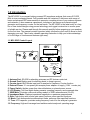
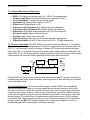
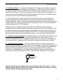
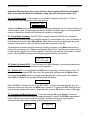
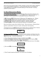
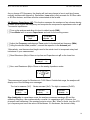
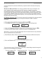
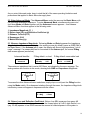
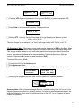
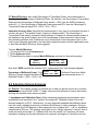
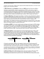
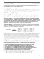
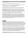
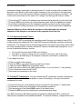
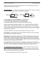
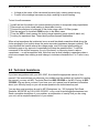
HF/VHF SWR Analyzer
Model MFJ-259C
INSTRUCTION MANUAL
CAUTION: Read All Instructions Before Operating Equipment
MFJ ENTERPRISES, INC.
300 Industrial Park Road
Starkville, MS 39759 USA
Tel: 662-323-5869 Fax: 662-323-6551
VERSION C1
COPYRIGHT
C
2013 MFJ ENTERPRISES, INC.
MFJ-259C Instruction Manual
HF/VHF SWR Analyzer
1.0 Introduction
The MFJ-259C is a compact battery-powered RF-impedance analyzer that covers 0.53-230
MHz in nine overlapping bands. Fully portable and self contained, it delivers a wide range of
basic and advanced RF measurements to present a complete picture of your antenna systems
and networks. It also measures capacitance, inductance, and serves as a discrete signal
generator and frequency counter for the test bench. The MFJ-259C is the latest entry in a long
line of time-tested designs using proven technology and rugged construction to ensure years
of reliable service. Please read through this manual carefully before powering up your analyzer
for the first time. The manual contains important safety information you'll need to know to avoid
damaging your unit. There's also valuable operating instruction to help you to take advantage
of its full range of functions and features right away.
1.1 MFJ-259C Control Layout
5
MFJ
POWER
6
3
1
2
FREQUENCY
COUNTER
INPUT
GROUND
POST
ANTENNA
MFJ HF/VHF SWR ANALYZER
MODEL MFJ-259C
4
GATE
POWER
13.8 VDC
7
9
8
SWR
IMPEDANCE
MODE
10
FREQUENCY MHz
67-113
11
113-155
155-230
28-67
11-28
Lower
Range
2.1-4.7 1.0-2.1
TUNE
4.7-11
12
0.53-1.0
1. Antenna Port: SO-239 for attaching antennas and RF devices under test.
2. Ground Post: Binding post for attaching leads to chassis ground.
3. Counter Input: BNC-female input jack for analyzer's Frequency Counter function.
4. External Power: 2.1-mm power jack accepts power adapter or supply (13.8V + center pin).
5. Power Switch: Applies power from internal batteries or external power source.
6. LCD Display: Two-line digital display presents operating frequency and measured data.
7. SWR Meter: Provides continuous analog readout of SWR measurements (Zo=50).
8. Impedance Meter: Displays impedance magnitude or reactance measurements.
9. Gate: Push button sets counter gate speed, performs other specified functions.
10. Mode: Push button selects measurement mode, performs other specified functions.
11. Tune: VFO capacitor, provides analog frequency control for the analyzer's generator.
12. Frequency: High and low-range band switches select analyzer's operating range.
2
MFJ-259C Instruction Manual
HF/VHF SWR Analyzer
1.2 Analyzer Measurement Functions
•
•
•
•
•
•
•
•
•
•
•
•
SWR: LCD display and analog meter, Zo = 50Ω or Zo programmable
Complex Impedance: Resistive and Reactive components (R ±jX)
Vector Impedance: Z-magnitude plus Phase Angle
Impedance (Z): Analog meter display, Zo=50 Ω
Return Loss: Digital display, in dB
Inductance (uH), Reactance (XL): Digital display with frequency
Capacitance (pF), Reactance (Xc): Digital display with frequency
Resonance: Digital and analog reactance null (X=0) with frequency
Electrical Length: Digital, measured in feet.
Feedline Loss: Digital, measured in dB
Signal Frequency: Discrete counter function with three gate speeds
Signal Generation: 20-mW (3-Vpp) output into 50 Ω, > -25 dBc suppression.
1.3 Theory of Operation: The MFJ-259C has four basic electronic elements. (1.) A tunable
VFO with counter readout that generates RF signals to energize the load or device under test
(DUT). (2.) A Directional Coupler (or bridge) to measure RF incident and reflected voltages
sent to the load. (3.) A Central Processor that reads bridge voltages and processes them into
usable data. (4.) A LCD Display and two analog meters that present all computed data visually.
The processor also performs other mathematical calculations and conversions.
Ant Jack
Tune
LCD
Display
VFO
Bridge
Load
(DUT)
A/D Converter and Processor
Meters
The MFJ-259C will serve as your eyes and ears when working with RF systems. However, all
handheld analyzers share certain limitations, and being aware of them will help you to achieve
more meaningful results.
1.4 Local Interference: Like most hand-held designs, the MFJ-259C uses a broadband
directional coupler that is open to incoming signals across the radio spectrum. Most of the
time, the unit's built in +5-dBm RF generator is powerful enough to override any interference
caused by stray pickup. However, under some circumstances, a powerful nearby transmitter
could inject enough RF energy through the antenna being tested to overload the coupler and
disrupt readings. If overload occurs, measurements may become erratic or SWR readings
inaccurately high. These occurrences are rare, but if it becomes a problem at your particular
testing location, the MFJ-731 Tunable Analyzer Filter is especially designed to notch out
unwanted signals with minimal impact on analyzer accuracy.
3
MFJ-259C Instruction Manual
HF/VHF SWR Analyzer
1.5 Calibration Plane: Your analyzer's Calibration Plane is the point of reference where all
measurements have greatest accuracy (Gain Reference = 0dB and Phase Shift = 0 degrees).
For basic handheld units like the MFJ-259C, the calibration plane is always fixed at the
analyzer's RF connector. Any time a transmission line is installed between the analyzer's RF
connector and an item being tested, the cable will displace the load from the calibration plane
and introduce some form of measurement transformation.
For SWR measurement, installing lengths of feedline usually causes a slight reduction in
readings caused by attenuation losses. Unless the cable losses are high, the difference is
usually insignificant. However, when documenting the performance of a new antenna design or
network device, the analyzer should always be connected as close to the load as possible to
minimize padding down of SWR readings.
Displacement of the calibration plane becomes far more significant when measuring
impedance because of phase rotation and transformer action occurring in the feedline. In fact,
impedance readings may swing dramatically, depending on the cable's electrical length and
the severity of the load's mismatch referenced to 50 Ohms. To collect meaningful impedance
data for a device, always connect the analyzer directly -- using the shortest cable possible.
1.6 Reactance Sign Ambiguity: Most handheld analyzers, including the MFJ-259C, lack the
data processing capability required to calculate Reactance Sign. These signs are (+) for
inductive reactance XL and (-) for capacitive reactance Xc. In most cases, you can apply one
or more simple tests to determine sign. See specific measurement instructions for details.
1.7 Protecting Your Analyzer: To minimize measurement error at high frequencies, the
analyzer's detector diodes are installed directly at the antenna port. Be aware that applying any
external potential exceeding a few volts of RF, AC, DC, or ESD energy could cause damage.
Caution and common sense are the best protections against failure. Never connect a
transmitter to the Antenna jack, and when testing ungrounded antenna systems that could
accumulate a static charge, always short the connector before attaching it to the analyzer.
Short Antenna
Leads to Discharge
Static Before
Connecting!
Important Warning: Never applying an external voltage to the Antenna jack -- it could
damage sensitive detector diodes. Also, always discharge the coax connector to bleed
off static before attaching ungrounded arrays.
4
MFJ-259C Instruction Manual
2.0
HF/VHF SWR Analyzer
Power Management
Read this section carefully -- supplying the wrong external voltage or failing to follow
battery installation procedures could result in permanent damage!
2.1 External Power Requirements: The MFJ-1312D AC adapter meets all technical
requirements for powering the analyzer and it is recommended. Any other external power
source must meet the following specifications:
•
•
•
•
•
Current: 250 mA or greater
Voltage Range: 11-16 VDC, well filtered (14 VDC ideal)
Battery Charging: 13.8 VDC minimum required for battery charger operation
Polarity: Negative ground only
Connection: 2.1-mm (+) center pin, (-) chassis ground (see below)
+
-
-
+
2.1 mm
2.2 Internal Battery Power: Always install fresh cells with identical part numbers and
expiration dates. For non-rechargeable power, install premium Alkaline cells and remove weak
cells immediately to prevent leakage. For rechargeable power, NiCds work well but Ni-MH cells
have no charge memory, hold a charge longer, and offer greater storage capacity. Before
loading new cells, always check (or know) the charger operating status -- is it On or Off ?
Important Warning: You must disable the analyzer's charger circuit when using nonrechargeable batteries, or destructive cell damage and chemical leakage may result.
2.3 Setting The Charger: Remove the analyzer's back cover (4 screws on each side of the
case). Find the upper left-hand corner of the main pc board and locate the 3-pin header J5
next to the power jack. A small black shorting plug is installed on the header.
Charger Off (non-rechargeable cells), install header on center and right pins as shown:
Charger On (rechargeable cells), install header on center and left pins as shown:
The charger provides a near-constant 20-mA/hr "trickle" rate any time external power is
applied. The Power switch need not be on for charging to take place. Charging depleted cells
may require 12 hours or more, so always allow enough time. Batteries will not over-charge.
5
MFJ-259C Instruction Manual
HF/VHF SWR Analyzer
Important Warning: Never store your unit more than a month with batteries installed.
Also, never ship with batteries installed or swap cells with the power switch "On"!
2.4 Low Voltage Alert: If the batteries (or external DC supply) drops below 11 Volts, a
flashing warning will appear on-screen (see below):
Voltage Low
10.5
Tapping the Mode button one time disables the warning and allows you to continue testing, but
measurements made at low voltage may not be reliable. If possible, plug in an external power
source or discontinue testing until batteries are replaced or recharged.
2.5 Sleep Mode (Standby): The MFJ-259C normally draws around 220 mA, consumed
mostly by the stimulus generator's amplifier stages. To extend battery life, your unit features a
built-in standby function called Sleep Mode. Sleep Mode shuts down signal generation and
reduces current drain to under 15 mA during periods of analyzer inactivity.
The analyzer's processor monitors activity by sensing activation of the Mode switch and by
looking for any change in the Tune control greater than 50 kHz. If neither event occurs during
a three-minute interval, the processor registers "inactivity" and switches into standby or Sleep
mode. A blinking SLP message on the display signals shutdown (see below):
10.125 MHz
R=42 X=12
1.3
SLP
2.6 Wake Up (Cancel SLP): To pull the unit out of SLP (standby), momentarily press either
the Mode or Gate button and resume normal operation.
2.6 Disable SLP: You may disable the SLP function manually if it interrupts your work. To
disable it, turn the analyzer Off, then turn it On again while holding down the Mode button.
Continue holding Mode until the copyright message appears on the screen, then release it.
When SLP is defeated, the message shown below will appear:
Power Saving Off
Note that SLP is a default function in the MFJ-259C -- it resets automatically each time you
power up unless you hold down the Mode key to defeat it. To restore the SLP function at any
time during an ongoing test session, simply turn the analyzer Off and then reboot it On again.
2.7 Powering-up (Boot) Sequence: To turn the analyzer On, press Power. Three boot
screens appear in sequence before the analyzer enters it's default SWR R&X measurement
mode. The first two screens show the analyzer's software version and copyright date
(important information when seeking technical assistance from MFJ):
MFJ-259C
Ver 13.40
MFJ Enterprises
©
6
MFJ-259C Instruction Manual
HF/VHF SWR Analyzer
The third screen provides a voltage check -- and flashes a warning if voltage is too low:
Voltage OK
14.2
Voltage Low 10.5
The fourth screen shows the operating frequency plus SWR and R&X impedance data. This is
the analyzer's default measurement mode. With no load connected to the Antenna jack, SWR
and Impedance (Z) will be very high, falling well outside the analyzer's normal measurement
range (greater than 25:1 and 650 Ohms):
10.140 MHz
R(Z>650)
>25
SWR
See Chapter-4.2 for complete measurement-mode R&X operating instructions.
3.0 VFO Frequency Control
The MFJ-259C's expanded-coverage VFO spans the LF, HF, and VHF spectrum from 0.53
MHz (AM broadcast) to 230 MHz (135-cm) in nine bands.
3.1 Band Switching and Tuning: Two Frequency MHz switches select high and low bands.
The High-Frequency band switch must be set fully clockwise to enable the Low-Frequency
band switch (see below).
FREQUENCY MHz
67-113
113-155
155-230
28-67
11-28
Lower
Range
2.1-4.7 1.0-2.1
TUNE
4.7-11
0.53-1.0
The VFO Tune capacitor features a reduction driver to provide smooth continuous frequency
control with a small amount of overlap at each band edge.
3.2 LF (630 Meter) Modification: You may shift LF-VFO coverage down to the experimental
630-Meter band (472-479 kHz). First rotate Tune counter-clockwise to its stop (lowest
frequency). Then, remove the back of the case (4 screws each side) and remove the battery
tray (2 screws on right side). Find the access hole for the 0.53-1.0 MHz tuning slug at the very
bottom-center of the pc board (only coil using a hex slug). Using a 2-mm insulated hex wand,
adjust the inductor while watching the LCD frequency display for 0.47 Mhz. Coverage should
now be ~0.47-0.94 MHz.
3.3 Signal Generator Function: You may use the output signal from the analyzer's internal
VFO as a discrete signal source (or signal generator) for testing purposes. Connect via the
SO-239 Antenna jack. Signal level is approximately 3-Vpp (20 mW into 50 Ohms or +5 dBm)
7
MFJ-259C Instruction Manual
HF/VHF SWR Analyzer
with all harmonics suppressed below -25 dBc. Although not phase-locked, stability is adequate
for most general alignment applications. To protect the bridge diodes from accidental DC
voltage applications, we strongly recommend installing an in-line attenuator or coupling
capacitor to provide isolation.
4.0 Basic Measurement Modes
4.1 The Basic Operating Menu: The MFJ-259C Basic Menu presents the analyzer's most
frequently used measurement functions. Tap the Mode switch to step through each one -- or
hold it down to scroll through them at a 3-second-per-screen rate. Selections are:
1. R&X: Measures SWR, R (Resistance), X (Reactance), Z (Z-magnitude), and (Phase).
2. Coax Loss (dB): Measures loss at any given frequency for 50-Ohm coax or a DUT.
3. Capacitance (pF): Measures component's reactance, computes capacitance.
4. Inductance (uH): Measures component's reactance, computes inductance.
5. Frequency (MHz): Counter mode, measures frequency of an external RF source
Each menu selection opens with an Identifier Screen*. After a brief pause, a Working Screen
appears to present data. The menu is circular, reverting back to the beginning.
*On analyzer boot-up, the R&X Working Screen appears without its identifier screen. However,
the Identifier Screen will appear when stepping or scrolling through the menu:
Impedance
R&X
4.2 Measuring SWR, R, X, Z, and : This default function measures and displays five of the
most widely used network parameters simultaneously. To access and view measured data for
SWR, R, X, Z, and , follow the checklist below:
[
[
[
[
] Turn on the analyzer and allow it to boot to the default mode (R&X).
] Adjust the Frequency switches and Tune control to the desired test frequency (MHz).
] Connect the feedine (or load) to the analyzer's Antenna jack.
] Read numerical Standing Wave Ratio (SWR) in the upper right-hand corner of the display:
10.120 MHz
R= 73 X=5
1.5
SWR
[ ] Also, read SWR on the analog panel meter display:
1 1.2 1.5 2.0 2.5
3
SWR
[ ] Read Complex Impedance (R and X) on the bottom line of the display:
8
MFJ-259C Instruction Manual
HF/VHF SWR Analyzer
10.120 MHz
R= 73
1.5
X=10
[ ] Read Impedance Magnitude (Z) on the analog meter scale.
0 10 20 40 50 70 100 400
Ohms
[ ] Read Impedance Magnitude (Z) and Phase Angle ( ) presented numerically by pressing
and holding the Gate button. The LCD display changes, as shown below:
10.120 MHz 1.5
Z= 75
= 5° SWR
[ ] Release Gate to revert back to R&X.
Note that Reactance readings (X) could be inductive (+ XL) or capacitive (- Xc) because the
processor can't calculate the sign. However, you can often find the sign by installing a small
capacitor across the feedline connector to add a few ohms of capacitive reactance. If your
capacitor increases X, the load is likely capacitive (-) because your reactance added to it. On
the other hand, if your capacitor caused X to decrease, the load is likely inductive (+) because
it cancelled out some of the X. To ensure accuracy, keep the amount of Xc you add as small
as possible.
Also, when measuring through a feedline, always remember the values for R, X, Z, and are
displaced values measured at the analyzer's calibration plane and do not represent the actual
impedance of the device connected at the far end. To read the impedance of the device under
test accurately, you must connect directly to the DUT using the shortest leads possible (or use
an electrical half-wave of 50-Ohm cable) .
4.3 Measure Coax Loss (dB): This mode displays the Measured Loss in dB at the VFO
operating frequency for any length of 50-Ohm coax cable. It will also measure losses incurred
through 50-Ohm attenuators, transformers, or baluns. To measure Loss:
[
[
[
[
[
[
] Turn on the analyzer and allow it to boot to the default mode (R&X).
] Press Mode once to access Coax Loss and wait for the working screen.
] Adjust the Frequency switches and Tune control to the desired test frequency (MHz).
] Connect the feedine under test (or 50-Ohm device) to the Antenna jack.
] Make sure the far end of the coax or the output port of the device is unterminated.
] Read Coax Loss on the lower line of the LCD display:
10.120 MHz
Coax Loss = 2.1 dB
9
MFJ-259C Instruction Manual
HF/VHF SWR Analyzer
As you change VFO frequency, the display will track any change in loss in real time (losses
normally increase with frequency). Remember, Loss mode is only accurate for 50-Ohm cable
or 50-Ohm devices, and these must be unterminated at the far end.
4.4 Measure Capacitance (pF): This function measures the reactance of an unknown device
in Ohms (X) at a given test frequency and computes the component's capacitance value in pF.
To measure capacitance:
[ ] Turn on the analyzer and allow it to boot to default mode (R&X).
[ ] Press Mode twice to access Capacitance and wait for the working screen.
Capacitance
in pF
10.120 MHz
C(Z)>650 Xc
[ ] Adjust the Frequency switches and Tune control to the desired test frequency (MHz).
[ ] Using the shortest leads possible*, connect the capacitor to the Antenna jack.
*Alternatively, use the same lead length used in the actual circuit to incorporate stray lead
inductance in your measurement.
[ ] Read Reactance (Xc) in Ohms on top line and Capacitance in pF on the lower line:
3.500 MHz
C= 642 pF
71
Xc
[ ] Also, read Reactance (Xc) in Ohms on the analog Impedance meter:
0 10 20 40 50 70 100 400
Ohms
The measurement range for Reactance is 7-650 Ohms. Outside that range, the analyzer will
display one of the following error messages:
Too low to measure (X<7)
3.500 MHz
Xc
C (X<7)
Series-resonant (X=0) Too high to measure (Z>650):
3.500 MHz
C (X=0)
Xc
3.500 MHz
C (Z>650) Xc
Sign Ambiguity: In capacitance mode, the analyzer measures reactance (X) and the
operating frequency, then mathematically converts it to capacitance (pF). However, the
processor can't determine if the reactance sign is minus (-Xc). When in doubt, tune the VFO
up in frequency and see if the value of X decreases. If it decreases, the device is likely
10
MFJ-259C Instruction Manual
HF/VHF SWR Analyzer
capacitive because the reactance exhibited by a capacitor tends to decrease as frequency
increases.
Standard vs. Measured Values: Even though a Standard Value may be stamped on the
case, a capacitor rarely measure that value at RF because of ambient temperature,
manufacturing tolerances, and differences in the test frequency. The sensitivity to frequency
occurs because stray inductance compounding inside the device and along the leads running
to the analyzer's calibration plane form a series-LC circuit. Normally, this condition causes a
capacitor's value (in pF) to increase with frequency, and it may even reach infinity if the circuit
becomes series-resonant (X=0).
4.5 Measure Inductance (uH): This function measures the reactance of an unknown inductor
in Ohms (X) at a given test frequency and computes inductance in uH. To measure
inductance:
[ ] Turn on the analyzer and allow it to boot to default mode (R&X).
[ ] Press Mode three times to access Inductance and wait for the working screen.
Inductance
in uH
100.000 MHz
L(Z)>650
[ ] Adjust the Frequency switches and Tune control to the desired test frequency (MHz).
[ ] Using the shortest leads possible, connect the inductor to the Antenna jack.
Alternatively, you may use the same lead length used in the actual circuit so stray inductance
will be incorporated into the measurement.
[ ] Read Reactance (XL) in Ohms on top line, and read Inductance in uH on the lower line:
100.000 MHz
76
[ ] Also, read Reactance (XL) in Ohms on the analog Impedance meter:
0 10 20 40 50 70 100 400
Ohms
The measurement range for Reactance is 7-650 Ohms. Values falling outside that range will
prompt one of the following error messages:
Too low to measure (X<7)
100.000 MHz
XL
L (X<7)
Parallel-resonant (X=0)
100.000 MHz
XL
L (X=0)
Too high to measure (Z>650)
100.000 MHz
L (Z>650) XL
11
MFJ-259C Instruction Manual
HF/VHF SWR Analyzer
Sign Ambiguity: In Inductance mode, the analyzer measures reactance (X) and the operating
frequency, and then mathematically computes Inductance in uH. However, the processor can't
determine if the reactance sign is positive (+XL). When in doubt, tune the VFO up in frequency
and see if the value of X increases. If it does increase, the device is likely inductive because
reactance exhibited by an inductor normally increases with frequency.
Standard vs Measured Value: The Standard Value for most inductors is determined at low
frequency (often in the kHz region). At RF, the value in uH may measure substantially different
because of stray capacitance between windings and other parasitic influences such as lead
capacitance or even the coil's proximity to other objects. Typically, the value in uH will increase
with frequency as the device moves closer to self-resonance. At self resonance, the inductor
looks like an open circuit (or a trap), exhibiting infinitely high reactance. Conversely, at some
very low frequency, it may look like a dead short.
4.6 Frequency Counter Mode: This function makes the analyzer's frequency readout circuitry
available as a discrete frequency counter for your test bench. Like many counters, sensitivity
for "locked-up" readings gradually decreases at higher frequencies. At HF, the measurement
threshold is under 10 mV-pp, but gradually increases to nearly 200 mV-pp at 230 MHz. The
"never-exceed" input voltage for safe testing is 2.0 V-pp.
Important Warning: Never exceed 2-Volts peak-to-peak or apply a DC voltage to the
Counter Input. Also, never connect a transmitter or unknown signal source to the input.
To access the counter function:
[ ] Turn on the analyzer and allow it to boot to default mode (R&X).
[ ] Press Mode four times to access Freq. Counter and wait for the working screen.
000.000 MHz 0.1s
Freq. Counter
Freq. Counter
[ ] Connect your signal source to the BNC-Female Frequency Counter Input connector.
[ ] Read Frequency in MHz and Gate time in seconds (0.1s) on the top line of the display.
146.700 MHz 0.1s
Freq. Counter
The default gate speed is 0.1 second, providing 1-kHz resolution. Other options are .01
second (very fast gate) with 10-kHz resolution and 1.0 second (slow gate) with 100-Hz
resolution. To change the Gate speed:
[ ] Press Gate once for .01-sec gate time. Two screens appear in rapid succession:
Gate Time .01s
146.70
.01s
Freq. Counter
12
MFJ-259C Instruction Manual
HF/VHF SWR Analyzer
[ ] Press Gate again for 1.0-sec gate time:
Gate Time 1.0s
146.7000MHz 1.0s
Freq. Counter
To return to the 0.1-sec default speed, press Gate again. Note that response time to
commands entered in the 1.0-sec gate setting is very slow. It may take several seconds for the
function to come up initially and several more seconds before it will respond to the command
to return to default.
5.0 Advanced Measurements
5.1 Introduction: The Advanced Menu provide accurate Distance to Fault measurement for
pinpointing transmission line problems in Feet. It also provides Resonance detection, useful for
quickly identifying the exact frequencies where X=0. In addition, it measures Impedance
Magnitude (Z, ) as the primary display function -- eliminating the requirement to press and
hold down the Gate switch when making those measurements.
Finally, Advanced mode measures Return Loss, Reflection Coefficient, and Match Efficiency,
all engineering parameters directly related to SWR. Note that, for general antenna work, SWR
remains the most universally applied measure of array performance -- and it is really the only
data needed to get most jobs done. Advanced terms address SWR from different technical
perspectives and applying them correctly usually requires a deeper understanding of RF
engineering principles. For reference purposes, the chart below illustrates how these and other
advanced engineering concepts all equate directly to the basic SWR measurement:
13
MFJ-259C Instruction Manual
HF/VHF SWR Analyzer
As you enter Advanced mode, keep in mind that all of the same operating limitations and
precautions that applied in Basic Menu also apply here.
5.2 Enter Advanced Mode: The Advanced Menu works the same as the Basic Menu, with
five functions arranged in sequence. To enter Advanced Mode, simultaneously press and
hold down Mode and Gate together until the Advanced screen appears -- then release.
Advanced Menu functions appear in the following order:
1. Impedance Magnitude (Z, )
2. Return Loss (RL) and Reflection Coefficient (ρ)
3. Distance To Fault (DTF)
4. Resonance (X=0)
5. Match Efficiency (η)
5.3 Measure Impedance Magnitude: Releasing Mode and Gate bypasses the Impedance
Magnitude identifier screen and displays the working screen by default (same as SWR R&X in
the Basic Menu). If the Antenna jack is open, the display will show a high-impedance "out-ofrange" message. If a measurable load is connected to the Antenna jack, the normal Z-Mag
data screen appears (see below):
Advanced Identifier
Z-Mag default, no load
10.140 MHz
R(Z>650)
Advanced
Z-Mag default, measurable load
10.120 MHz 1.5
Z= 75
= 5° SWR
>25
SWR
The maximum impedance limit is set at 650 Ohms, as indicated by the error message. The
analog meters also function in this mode, showing both SWR and Impedance Magnitude:
1 1.2 1.5 2.0 2.5
SWR
3
0 10 20 40 50 70 100 400
Ohms
To access the other Advanced menu selections, simply step or scroll past the Z-Mag function
using the Mode switch. On subsequent rotations through the menu, the Impedance Magnitude
introductory screen will appear in sequence with the others:
Impedance
Z = Mag,
= Phase
5.4 Return Loss and Reflection Coefficient: Return Loss (RL) measures how many dB
down the reflected wave is when referenced to the forward wave at 0-dB. A high Return Loss
(say -25 dB) equates to low SWR because the amount of reflected power in the system is
14
MFJ-259C Instruction Manual
HF/VHF SWR Analyzer
minimal compared to forward power. A smaller number (-9.5 dB) equates to higher SWR (~
2:1) because the difference between forward and reflected power is less. Reflection Coefficient
(ρ) expresses the voltage relationship between the reflected wave and the forward wave on a
scale of 0 to 1.0. A Reflection Coefficient of 0.2 is approximately equal to 1.5:1.
To access and view measured data for Return Loss (RL) and Reflection Coefficient (ρ):
[
[
[
[
[
] Turn on the analyzer and allow it to boot to the basic system default mode (R&X).
] Connect the DUT to the Antenna jack
] Press Mode and Gate together until Advanced appears on-screen, then release.
] Press Mode once to access Return Loss & Reflection Coeff.
] Wait for the working screen.
Return Loss &
Reflection Coeff
14.150
1.3
RL=18 ρ=.13 SWR
[ ] Adjust the Frequency switches and Tune control to the desired test frequency (MHz).
[ ] Read numerical Return Loss (RL), (SWR), Reflection Coefficient (ρ) on the display:
[ ] Read Impedance and SWR on the analog meters.
5.5 Distance To Fault: In DTF mode, you can measure the physical length of a random run of
cable or find the distance to a fault in a transmission line. To do it, you'll first measures the
electrical distance to the abnormality (or the cable end), then multiply it times Velocity Factor to
get a physical distance in feet. At the far end of the cable, open and shorted terminations yield
the best accuracy (resistive or reactive terminations can skew results or fail to test). You may
also test balanced line using this method, but it requires a special procedure to keep the line in
balance and isolated from ground (see below). Coax can be tested in any configuration.
Balanced Line: To avoid proximity errors, twin-lead, window line, ladder line, and open-wire
feeders needs to be suspended in a straight line in the air and a few feet away from earth or
other conductors. The analyzer must also be isolated from proximity to ground by running on
internal battery power with only the feedline under test attached. One leg connects to the
Antenna jack center pin and the other goes to the analyzer ground stud or connector flange.
To measure fault distance:
[ ] Connect the DUT to the Antenna jack
[ ] Enter Advanced Mode
[ ] Press Mode twice to access Distance To Fault. Wait for the working screen:
Distance to Fault
in feet
5.0000MHz 1st
DTF
X=23
The top line shows Frequency and a blinking "1st" prompt. The lower line shows Reactance.
To find electrical length, you'll find and enter two consecutive frequencies where (X=0).
[ ] Using the VFO, search for the lowest frequency you can find where the Impedance meter
shows a sharp null and the display shows X=0 (or as close to 0 as possible).
[ ] Press Gate to enter that frequency. The display will switch to the 2nd prompt
15
MFJ-259C Instruction Manual
HF/VHF SWR Analyzer
3.8944MHz 2nd
DTF
X=0
3.8944 MHz 1st
DTF
X=0
[ ] Tune the VFO higher in frequency to find the next X=0 null (or close as possible to 0).
11.519 MHz 2nd
X=2
DTF
[ ] Press Gate to enter second frequency. Display will show:
Dist. to fault
64.0 ft x Vf
[ ] Multiply DTF x Velocity Factor of the cable (Vf) to get the physical distance in feet.
(64.0 x .66 = 42.24)
The cable length (or the distance to a "fault" in a longer cable) is 42.24 feet, or 42' 3".
5.6 Resonance Mode: Resonance mode works exactly the same as R&X in the Basic Menu,
except the analog Impedance Meter displays Reactance rather than Impedance Magnitude.
This change makes it easier to spot nulls and pinpoint the frequencies where Resonance
occurs. Resonance is defined as the frequency where Capacitive Reactance (Xc) and
Inductive Reactance (XL) cancel out and equal zero (X=0).
To access Resonance Mode:
[ ] Connect the DUT to the Antenna jack
[ ] Enter Advanced Mode
[ ] Press Mode three times to access Resonance Mode and wait for the working screen:
Resonance Mode
tune for X=0
14.150 MHz
R=54 X=4
1.5
SWR
[ ] Watching the Impedance meter, tune for a null (X=0 or as close as possible).
0 10 20 40 50 70 100 400
14.168 MHz
OhmsR=54 X=0
1.5
SWR
Accuracy Note: When measured thought feedline, the X=0 reading many not occur on the
frequency where the antenna is actually resonant. As with any reactance measurement, the
analyzer Calibration Plane must be positioned close to the DUT (or to 0-degrees of phase
rotation) as possible.
16
MFJ-259C Instruction Manual
HF/VHF SWR Analyzer
5.7 Match Efficiency: Also called Percentage of Transmitted Power, this measurement is
directly related to Percentage of Reflected Power. By definition, the Percentage of Transmitted
Power plus the Percentage of Reflected Power equals = 100% (see the SWR equivalency
chart at 5.1). If the Percentage of Reflected Power measures 25%, then the Percentage of
Transmitted Power will equal 75% (100% - 25% = 75%).
Important Accuracy Note: Note that this measurement is very easy to misinterpret because it
contains the word "Transmitted Power" (implying "radiated power"). The Percentage of
Transmitted Power simply represents the percentage of forward vs. reflected power present in
the feedline at any given moment, and not the percentage of the transmitter's output power
that ultimately performs work. Reflections occur at both ends of the transmission line, so the
"real" power ultimately absorbed by the load after multiple bounces could be significantly more
or less than the Match Efficiency value suggests!
To enter Match Efficiency:
[ ] Connect the DUT to the Antenna jack
[ ] Enter Advanced Mode
[ ] Press Mode four times to access Match Efficiency and wait for the working screen:
Match
Efficiency
14.150 MHz
1.4
Match = 94% SWR
Note that if SWR exceeds the analyzer's 25:1 measurement limit, this message appears:
29.538
>25
Percentage of Reflected Power: To calculate
Percentage
of Reflected Power from Match
Power< 15% SWR
Efficiency, simply subtract the Match Efficiency from 100%: Using the example above, %
Reflected Power = (100% - 94%) = 4%.
6.0 Adjusting Simple Antennas
6.1 General: This chapter focuses on practical tips to help you get the most from your backyard antennas using the MFJ-259C. To begin, here are some pointers to keep in mind when
working with amateur radio antenna system:
1. Impedance and Calibration Plane: When measuring impedance and reactance, we've
emphasized how important it is to "position" the analyzer's Calibration Plane close to the
element feedpoint (or DUT). Alternatively, you may physically separate the calibration plane
from the load by installing a precisely cut electrical half-wave of cable in between. Doing so
rotates phase a full 360 degrees so there appears to be no phase shift ( = 0°) or impedance
transformation (Z) error. This strategy works well, but is a "single frequency" solution. Even a
small excursion (more than ± 2° of phase shift) from the cable's "cut" frequency will skew
impedance readings as the cable becomes non-resonant and begins to reintroduce its own
17
MFJ-259C Instruction Manual
HF/VHF SWR Analyzer
reactance into the system. Phase errors compound with multiple half-waves, so it's best to limit
length to one or two phase rotations.
2. SWR, Resonance, and Impedance: Always use SWR rather than Resonance (X=0) or
Impedance magnitude (Z) to optimize simple antennas. SWR is much easier to measure
accurately because feedline length and calibration plane placement aren't critical. Also, if you
cut the element based on Resonance alone (X=0), a significant resistive mismatch may still be
present that shifts minimum SWR elsewhere. And, if you cut for Z=50 Ohms alone, you may
get a large reactive component yielding the same outcome. SWR is always your best bet.
3. Tuning vs Matching: Unlike simple wire dipoles or verticals, many antennas have a built-in
impedance matching networks (Delta, Gamma, Shunt, etc). These antennas may be adjusted
for both resonance and impedance. Begin by setting up the prescribed element length for your
target frequency using the manufacturer's instruction sheet, a model, formula, or X=0
measurement. Then, adjust the antenna's matching network for minimum SWR. In most cases,
the two adjustments will interact, so be prepared to alternately touch them up. Again, minimum
SWR at your target frequency should be the last word.
4. Feedline and SWR: If all is well, feedline length won't have much impact on SWR readings.
You should be able to add or remove cable or measure SWR at any point along the way with
little change. It's normal to see a small SWR drop when adding cable or an increase when
removing it because of resistive loss. But, if you see big SWR changes when altering feedline
length, repositioning the cable, or grounding the shield at any point, suspect a problem.
5. Radiating Feedlines: Common-Mode RF Current flowing along the outer surface of the
coax shield is always be a prime suspect when you see erratic SWR changes. It happens
when the feedline becomes part of the antenna element and radiates RF (hence the sensitivity
to cable length, positioning, and grounding). With a radiating feed, it's virtually impossible to
measure the antenna's actual resonant frequency or SWR because the load presented by the
feedline alters these parameters unpredictably.
With no balun,
"dipole" actually
has three legs.
Balun "chokes off"
the third RF path
A Guanella current balun installed at the feedpoint offers the best protection against RF
conducting down the outside of the cable. The balun functions as a choke to isolate the coax
shield from the part of the antenna that's supposed to be radiating. It's also important to run
coax away from the antenna at a 90-degree angle to prevent RF from coupling onto the line by
induction. These two steps not only stabilize SWR, they reduce receiver noise, get rid of RF in
the shack, and allow the antenna to radiate predictably.
6. Defective Cable: Erratic SWR readings will also occur if your coax isn't 50 ohms. Kinks,
water ingress, oxidation, corrosion, bad connectors, improper construction, and even
mislabeling by the manufacturer may be the cause. Check SWR with a dummy load installed
18
MFJ-259C Instruction Manual
HF/VHF SWR Analyzer
at the far end of the cable. If it is elevated or the Impedance (Z) fluctuates very much as you
tune the analyzer's VFO, suspect defective cable.
7. Lossy Cable: Coax may exhibit excessive loss from contamination or may have too much
normal attenuation for use at higher operating frequencies. To measure loss, unhook the cable
and use the analyzer's Coax Loss mode to check it against the factory specifications.
6.2 The Coax-Fed 1/2-Wave Dipole:
Baluns (again): The 1/2-wave dipole is a balanced radiator and coaxial cable represents an
unbalanced feed system, so it's especially important to install a balun at the feedpoint. Your
balun could be a number of turns of coax wrapped into a coil several inches in diameter and
taped to the feedpoint, or it could be a complicated affair with many interconnecting windings
on a ferromagnetic core. The best choice is a simple 1:1 Guanella "current" balun wound on a
toroid core made from material with the appropriate permeability (43-Mix preferred for most HF
applications). If the feedline isn't isolated, it may load the element and impact a number of
parameters -- including your calculations for the correct element length.
Tuning to Frequency: A dipole's minimum-SWR frequency is mainly determined by element
length. If it's too long, minimum SWR will occur below the target frequency. If too short, it will
occur above. The formula for length is shown below:
Length in Feet =
468
Freq. in MHz
1.85 Mhz = 253'
1.925 MHz = 243'
7.15 MHz = 65' 5"
10.12 MHz = 46' 3"
21.25 MHz = 22'
24.93 MHz = 18' 9"
3.6 MHz = 130'
3.85 MHz = 121' 7"
14.25 MHz - 32' 10"
18.11 MHz = 25' 10"
28.5 MHz = 16' 5"
50.15 MHz = 9' 4"
Length is primary, but other factors may also enter in. "Fat" wire or larger tubing tends to lower
the frequency below formula by introducing capacitive loading. Dipoles made with jacketed
wire may resonate low because the velocity of propagation (Vp) is slowed by the insulation.
Ground conductivity, soil moisture, proximity to other wires, nearby structures, and metal
surfaces also have an impact. And, some specific types of dipoles (inverted "V", NVIS, OCFD,
etc) may tune a little differently because of how they are configured.
Scaling: With so many variables, it's usually better to cut your antenna 5%-10% longer than
formula, put it up, measure the SWR, and calculate a Scaling Factor to nail down the exact
length you need at your specific location. To scale for length, follow this procedure:
[
[
[
[
[
[
[
] Calculate element length, then multiply the result x1.05 to make it 5% longer.
] Built it, then measure and write down the exact length in feet. Call it L1.
] Put the antenna up in the location where you intend to install it permanently.
] Set the analyzer for SWR (R&X) and tune the VFO for the minimum SWR reading.
] Write down the minimum SWR frequency as FR (reference frequency).
] Write down the target operating frequency as FT (target frequency)
] Calculate a Scaling Factor (SF) to determine the amount of change needed:
If FR is a lower frequency than FT, let SF = FT/FR. (scaling factor <1.0).
If FR is a higher frequency than FT, let SF = FR/FT (scaling factor >1.0).
19
MFJ-259C Instruction Manual
HF/VHF SWR Analyzer
[ ] Calculate the new (target) antenna length (L2) as follows: L2 = L1 x SF.
Example: Your 132-foot dipole has minimum SWR at 3.750 Mhz. You want it at 3.900 MHz.
The element is presently too long, so: SF = FT/FR = 3.750/3.900 = 0.96.
The new length will be: L2 = L1 x SF = 132' x .96 = 126.7'.
Scaling eliminates time-consuming "cut-and-try", but it only works on full-size dipoles and
verticals with no loading coils, matching networks, traps, stubs, capacitance hats, etc.
Dipole Height: Dipole resistance is mainly influenced by proximity to ground. Most dipoles
match quite well through 50-Ohm coax at normal residential mounting heights (hence their
popularity). By altering height, you may be able to improve your match. However, don't let
SWR be your only consideration! If the change places too much stress on high tree branches
or changes the angle of radiation unfavorably (local vs DX), why change? A small
improvement in SWR will have little impact on your station's overall performance.
Radios, Impedance, and SWR: When antenna and feedline aren't precisely matched, we
know the coax will act like a transformer and modify the value of the load appearing at your
radio (same dynamic that applies to your analyzer's calibration plane). However, if you use
good-quality 50-ohm cable and set your station up properly, most solid-state radios have no
problem handling these impedance excursions as long as the SWR remains below 2:1. As
Section 6.1 pointed out, your SWR shouldn't change even though the impedance may shift
around because of phase rotation in the cable.
6.3 Verticals:
1/4-Wave Vertical: All 1/4-wave monopoles require a good ground system. If your radial
system is poor, the "good earth" will swallow up a large portion of your signal as ground loss.
In fact, you can often gauge the integrity of your radial field by measuring the antenna's driving
resistance (the value of R when X=0). It should be low -- around 25-35 Ohms. If your 1/4-wave
vertical shows a tidy 1:1 match through 50-Ohm cable, that's your cue to lay out more radial
wire. Radials placed on the ground need not measure exactly 1/4-wave to be effective, but a
minimum of 16 is recommended and more is always better. Antenna books cover radial
systems extensively, although not all authors may agree on the best way to construct them.
A 1/4-wave vertical tunes the same way as a dipole -- lengthen to lower operating frequency
and shorten to raise it. Monopole length can be scaled unless the element is loaded with a hat
or a loading coil. Because the impedance is (or should be) quite low, most require matching at
the feedpoint to make the transition up to 50 Ohms (shunt matching coil, L-network, autotransformer, etc.). HF monopoles with a good radial system underneath are efficient, have a
very low angle of radiation, and make excellent DX transmitting antennas.
Ground-Independent Verticals: These antennas don't require radial systems because they
have a counterpoise of some sort built in. Most are configured as multiband OCFDs (off-center
20
MFJ-259C Instruction Manual
HF/VHF SWR Analyzer
fed dipoles) with the longer leg being the dominant vertical radiator. The counterpoise is often
fanned out at the base as sloping radials or as a capacitive-hat structure. Ground-independent
verticals are really "dipoles" oriented in the vertical plane, and they tend to work more
efficiently when elevated well above ground. Mounted close to the soil, they tends to detune
and radiate less efficiency because of ground losses. Most are multi-band arrays with the
larger vertical radiator using resonant elements connected in parallel, traps installed in series,
or a combination of both. Also, most utilize a built-in matching network and balun at the
feedpoint to match into 50-Ohm coax. Tuning procedures may be somewhat complex and
interactive for arrays with multiple bands, so its important to follow the manufacturer's
procedure for tune up.
7.0 Special Measurement Procedures
7.1 Overview: There are a number of specialized measurement procedures you can follow to
extend the versatility of your MFJ-259C. These include the following tasks:
•
•
•
•
•
•
Measuring and cutting a transmission line stub to Electrical Length.
Measuring the Velocity Factor (Vf) of an Unknown Cable.
Finding the Impedance (Z) of an unknown feedline or Beverage antenna.
Pre-adjusting an antenna tuner.
Testing RF transformers and baluns for isolation.
Analyzing RF chokes for Self-resonance.
7.2 Measuring and Cutting a Line or Stub to Length: To cut a matching stub or a resonant
length of transmission line, use the analyzer's default SWR/Impedance function in the Basic
Menu (R&X).
[
[
[
[
] For 1/4λ and odd multiples (1/4λ, 3/4λ, 5/4λ, etc), terminate the cable with an open.
] For 1/2λ and even multiples (1λ, 1-1/2λ, 2λ), terminate with a short.
] Coaxial lines may be piled or coiled on the floor -- no isolation from ground needed.
] Balanced lines require isolation from ground. See the setup outlined in Chapter 5.5.
Next, determine your target frequency (FT) and estimate cable length as follows:
[
[
[
[
[
[
[
[
] Calculate 1λ in feet = (983.6 / Freq. MHz), or 1λ in inches = (11803 /Freq. MHz)
] Multiply 1λ by the fractional length you need (eg λ x .25 for 1/4λ, 1λ x .5 for 1/2λ, etc.)
] Look up or measure your cable's Velocity Factor (Vf)
] Convert the cable's Electrical Length to a Physical Length: LPH = LEL x Vf
] Cut the cable 20% longer than your calculated Physical Length: LCUT = 1.2 LPH
] Connect one end to the analyzer and terminate the other end as specified (short or open).
] Tune the analyzer VFO to find the frequency of the lowest Impedance null.
] Fine-tune, watching the Reactance (X) display. Adjust as close to X=0 as possible.
21
MFJ-259C Instruction Manual
HF/VHF SWR Analyzer
If calculations and the Vf accurate, your null should occur ~20% below the target frequency to
reflect the added length. Next, calculate a scaling factor to determine exact cut length. You've
initially cut the cable 20% "long and low", so your scaling factor will always be less than 1.0:
[ ] To find the Scaling Factor (SF), divide the null freq. F1 by the target freq. F2: (SF = F1/F2)
[ ] Multiply the Scaling Factor (SF) by the present physical length (SF x LCut) for a final length.
[ ] Cut the stub and confirm the new reactance null (X=0) is on your target frequency.
7.3 Measure Velocity Factor (Vf) of a Unknown Cable: Velocity of Propagation (Vp) and
Velocity Factor (Vf) are terms that express how fast RF propagates on a conductor relative to
the speed of light. Although the two terms are often used interchangeably, Velocity of
Propagation is usually given as a percentage (example: Vp = 66%) while Vf expresses the
percentage as a multiplier for making frequency and length calculations (example: Vf = .66). To
determine Velocity Factor (Vf) for a unknown transmission line:
[ ] Refer to DTF (Chapter 5.5) and find the Electrical Length of your cable in feet.
[ ] Follow the DTF procedure.
Your cable's Electrical Length will be the DTF result without a Vf calculated in to the resut (see
below). Label your result LEL (for Electrical Length).
Dist. to fault
64.0 ft x Vf
[ ] Using a tape or rule, measure the Physical Length of your cable in feet. Label it LPH.
[ ] Divide Physical Length by Electrical Length to find Velocity Factor: Vf = LPH / LEL.
Example: If the Electrical Length is 64 feet and the Physical Length is 42' 3" (42.25) feet, then
the measured Vf of the cable calculates 0.66: (42.25 / 64 = .66).
7.4 Impedance of a Transmission Lines or Beverage Antenna: This procedure measures
the Impedance of an unknown transmission line (or Beverage), from 7-650 Ohms. If needed,
the range may be extended using a broadband transformer or a known resistance. Use the
analyzer's Basic Mode (R&X) augmented by the Impedance Magnitude feature (Z) provided by
the Gate key.
Methodology: Transmission lines have a "characteristic impedance" (50 Ohms, 70 Ohms,
300, 450 Ohms, etc). When a line is terminated by a load of the same impedance, no
impedance transformation occurs between the near end and far end, regardless of electrical
length. However, if we introduce a mismatch at one end, the impedance at the far end cycles
above and below the cable's characteristic impedance with changing frequency.
22
MFJ-259C Instruction Manual
HF/VHF SWR Analyzer
j+X
R2 (High)
100 Ohms
180°
50 Ohm
Transmission
Line
R1 (Low)
25 Ohms
0°
Load = 100 Ohms
SWR = 2:1
Z=
R1 x R2
Z=
25 x 100
Z = 50 Ohms
j-X
Viewed on a Smith Chart, the transformed load impedance (R ±jX) literally traces a circle
around the characteristic impedance of the transmission line with each 360-degrees rotation.
The greater the mismatch, the larger the diameter of the circle. We can use this behavior in
two different ways to determine the impedance of an unknown transmission line.
One way is to intentionally introduce a resistive mismatch at one end of the line and measure
the amount of impedance transformation it causes at frequencies where X=0. As shown above,
for each full rotation there will be two Zero-Crossing Points where X=0 and the load becomes
purely resistive. One occurs below the line's characteristic impedance and the other above.
Using the high and low resistive values (R1, R2), we can calculate the impedance of the line.
Or, alternatively, we can connect a series of trial loads at the far end of the cable until we find a
value where the impedance excursions are reduced to zero (the line's characteristic
impedance).
When running these test, coax may be piled or coiled on the floor, but balanced lines must be
isolated as described in Chapter 5.5. Connect Beverage antennas directly to the analyzer.
Intentional Mismatch Method: To ensure accuracy, use a non-inductive load and choose a
value that holds the high and low impedance excursions well within the analyzer's accurate
measurement range (7-650 Ohms).
[
[
[
[
[
[
[
[
[
] Connect the cable to the analyzer and terminate the far end with the load you have chosen.
] Tune VFO for the lowest frequency where Impedance and Resistance indicators both dip.
] Fine tune to locate the point where X=0 and R are both at their minimum value.
] Press Gate to confirm θ = 0°. Write down the Resistance (R) reading as R1.
] Tune up in frequency to find a distinct Impedance peak.
] Fine tune to locate the point where X=0 and Resistance (R) peaks at maximum value.
] Press Gate to confirm θ = 0°. Write down this Resistance (R) reading as R2.
] Multiply R1 x R2 and find the square root of the product.
] The result is the characteristic impedance of your line.
Example: R1=36 ohms and R2 = 71 ohms, (36 x 71 = 2556), square root = 50.6 ohms.
If you wish to confirm the result, try other load values.
Load Substitution Method: At HF, use non-inductive fixed-value resistors, a physically small
carbon potentiometer or trimpot, a (compact) decade box, or a broadband transformer of
known accuracy (to extend range). Above HF, avoid any load that could introduce stray
23
MFJ-259C Instruction Manual
HF/VHF SWR Analyzer
inductance through lead length or internal structure. For best accuracy with a variable load,
disconnect and check its value with a digital ohmmeter at the conclusion of the experiment.
However, never check load resistance with an ohmmeter with the analyzer connected -- the
results will be inaccurate and the meter's DC voltage could damage the detector diodes!
[
[
[
[
] Connect the DUT cable to the analyzer and terminate the far end with your first trial load.
] Tune the VFO up and down over a wide frequency span. Note the Impedance changes.
] Try different terminations until the Impedance remains constant over the tuning range.
] The resistance holding Impedance most constant is the line's characteristic impedance.
Important Warning: Never check the resistance of an adjustable load using an
ohmmeter if the analyzer is connected at the opposite end of the line!
7.5 Pre-adjusting Antenna Tuners
Using the MFJ-259C to pre-adjust the impedance match through your station's tuner (ATU)
avoids exposing the transmitter PA to high-SWR loads and eliminates needless over-the-air
interference. The analyzer may be temporarily patched to the tuner's input using a short cable,
but many operators prefer to install a manual RF switch to facilitate rapid changeover. If you
choose to switch the analyzer, confirm:
• Your switch has more than 50 dB of port Isolation
• The wiper (or common) switch port is connected to the Input Jack of the tuner
• There's no possible way for the analyzer to become connected to a transmitter.
To pre-adjust the tuner:
[
[
[
[
[
[
] Patch or switch in the analyzer.
] Tune the VFO to your target frequency and leave it there
] Select the default R&X mode in the Basic menu.
] Adjust the tuner controls until SWR indicators show 1.0 (or as close to 1:1 as possible).
] Turn off and disconnect the MFJ-259C
] Reconnect the transmitter to the tuner.
7.6 Testing RF Transformers: You can evaluate any RF transformer that has a termination
port between 25 and 100 Ohms available on one of its windings. Use only non-inductive
resistances for loads:
[
[
[
[
] Connect the test port to the analyzer with a very short 50-ohm pigtail (<1° phase shift).
] Terminate all other port(s) with loads of the specified impedance.
] Set the analyzer to the default R&X function in the Basic menu.
] Sweep the VFO across the transformer's intended operating range.
Use SWR, Resistance (R) Reactance (X) and Impedance Magnitude (Z) to evaluate the
transformer's impedance and useable bandwidth. To measure efficiency, compare the source
24
MFJ-259C Instruction Manual
HF/VHF SWR Analyzer
voltage at the input port generated by the MFJ-259C to the load voltages at the other ports
using standard power-level conversions.
7.7 Testing Baluns: To evaluate the performance of "current" and "voltage" style baluns,
follow the outlined procedures referring to Figures A and B below:
Fig A
A
50 Ohms
Unbal
Balun
Fig B
R1
B
C
50 Ohms
Unbal
Clip Lead
[
[
[
[
<
Balun
R2
>
R1
A
C
R2
Clip Lead
] Set the analyzer to the default R&X function in the Basic menu.
] Set the VFO to the midpoint of the Balun's operating range
] Connect the analyzer to the balun's 50-ohm unbalanced input.
] Terminate the balanced side with equal-value load resistors as shown:
Use two equal-value non-inductive resistances. For a 4:1 balun with a 200-ohm secondary,
configure a pair of 100-ohm resistors in series. For a 1:1 balun with a 50-Ohm secondary,
connect 50-Ohm resistors in parallel to make a pair of 25-Ohm resistors, or if using standard
values, connect 47 and 56-Ohm resistors in parallel to make up 25.5 Ohm loads. To evaluate
your balun, refer to Figure-A:
[ ] Measure SWR while connecting the grounded clip lead to points A, B, and C.
Current Balun: A well-designed current balun will exhibit low SWR over its entire operating
range with the clip lead installed at A, B, or C.
Voltage Balun: A well designed voltage balun will exhibit low SWR over its operating range
with the clip lead installed at position B. However, it will show poor SWR with the clip lead
installed at A or C (elevated readings should be the same). To further test the voltage balun,
connect as shown in Figure-B. If operating properly, SWR will be remain low with the resistors
connected from either output terminal to ground.
A well-designed current balun works best for maintaining current balance on a dipole under
"real world" conditions where some asymmetry in loading may exist between the two legs. The
current balun also has the highest power capability and lowest loss for given materials.
7.8 Analyzing RF chokes for Self-resonance: Large RF chokes often have frequencies
where the distributed capacitance and inductance form a low impedance series-resonance.
Series resonance occurs because the choke winding acts like a succession of back-to-back Lnetworks. This condition can lead to three problems:
•
End-to-end Impedance of the choke becomes very low.
25
MFJ-259C Instruction Manual
•
•
HF/VHF SWR Analyzer
Voltage at the center of the resonance becomes high, causing severe arcing.
Current in the windings becomes very high, resulting in severe heating.
To test for self-resonance:
[
[
[
[
[
[
] Install and test the choke in its normal operating location to incorporate stray capacitance.
] Disconnect any choke leads leading to associated circuitry.
] Connect the analyzer to both ends of the choke using a short 50-Ohm jumper.
] Set the analyzer for its default R&X function in the Basic menu.
] Tune the VFO to slowly sweep the choke's target operating range (specific band, etc).
] Looking for impedance dips. These identify series-resonant frequencies.
When a low-impedance dip is detected, move a small insulated screwdriver blade along the
choke windings to find a point where the series-resonate impedance changes suddenly. This
jump identifies the location where the voltage peaks, and it's the spot where adding or
subtracting even a tiny amount of capacitance will have the greatest effect. To shift the
resonance off the critical frequency (or out of the band), try removing turns to reduce
capacitance -- or add a capacitive stub. Note that even a small change in capacitance has a
much more impact than making a small change in inductance because the L to C ratio is very
high.
8.0 Technical Assistance
If you have any problem with your MFJ-259C, first check the appropriate section of this
manual. If the manual does not reference your problem and the problem isn't solved by reading
the manual, you may call MFJ Technical Service at 662-323-0549 or the MFJ Factory at 622323-5869. We can serve you best if you have your unit, manual, and all pertinent information
about your difficulty handy so you can answer questions the technicians may ask.
You can also send questions by mail to MFJ Enterprises, Inc., 300 Industrial Park Road,
Starkville, MS 39759; by FAX to 662-323-6551; or by e-mail to [email protected].
Send a complete description of your problem, an explanation of exactly how you are using
your unit, and a complete description of your station.
26
MFJ-259C Instruction Manual
HF/VHF SWR Analyzer
LIMITED 12 MONTH WARRANTY
MFJ Enterprises, Inc. warrants to the original owner of this product, if manufactured by MFJ Enterprises, Inc. and
purchased from an authorized dealer or directly from MFJ Enterprises, Inc. to be free from defects in material and
workmanship for a period of 12 months from date of purchase provided the following terms of this warranty are
satisfied.
1.
The purchaser must retain the dated proof-of-purchase (bill of sale, canceled check, credit card or money
order receipt, etc.) describing the product to establish the validity of the warranty claim and submit the
original or machine reproduction of such proof of purchase to MFJ Enterprises, Inc. at the time of warranty
service. MFJ Enterprises, Inc. shall have the discretion to deny warranty without dated proof-of-purchase.
Any evidence of alteration, erasure, or forgery shall be cause to void any and all warranty terms
immediately.
2.
MFJ Enterprises, Inc. agrees to repair or replace at MFJ's option without charge to the original owner any
defective product under warrantee provided the product is returned postage prepaid to MFJ Enterprises,
Inc. with a personal check, cashiers check, or money order for $7.00 covering postage and handling.
3.
This warranty is NOT void for owners who attempt to repair defective units. Technical consultation is
available by calling the Service Department at 662-323-0549 or the MFJ Factory at 662-323-5869.
4.
This warranty does not apply to kits sold by or manufactured by MFJ Enterprises, Inc.
5.
Wired and tested PC board products are covered by this warranty provided only the wired and tested PC
board product is returned. Wired and tested PC boards installed in the owner's cabinet or connected to
27
MFJ-259C Instruction Manual
HF/VHF SWR Analyzer
switches, jacks, or cables, etc. sent to MFJ Enterprises, Inc. will be returned at the owner's expense
unrepaired.
6.
Under no circumstances is MFJ Enterprises, Inc. liable for consequential damages to person or property by
the use of any MFJ products.
7.
Out-of-Warranty Service: MFJ Enterprises, Inc. will repair any out-of-warranty product provided the
unit is shipped prepaid. All repaired units will be shipped COD to the owner. Repair charges will be
added to the COD fee unless other arrangements are made.
8.
This warranty is given in lieu of any other warranty expressed or implied.
9.
MFJ Enterprises, Inc. reserves the right to make changes or improvements in design or manufacture
without incurring any obligation to install such changes upon any of the products previously
manufactured.
10.
All MFJ products to be serviced in-warranty or out-of-warranty should be addressed to:
MFJ Enterprises, Inc.,
300 Industrial Park Road
Starkville, Mississippi 39759 USA
and must be accompanied by a letter describing the problem in detail along with a copy of your dated
proof-of-purchase.
11.
This warranty gives you specific rights, and you may also have other rights which vary from state to state.
2