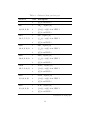
Download PyPES Library Manual

2
Setup and usage
PyPES requires the following programs and packages to be properly installed and configured:
• Python 2.7+ or Python 3.0+
• SciPy 0.13.2+
• NumPy 1.8.0+
• SymPy 0.7.4.1+
• Cython 0.21+
PyPES has been tested with Python 2.7.6 and 3.4.1, with the packages listed above. PyPES
should be compatible with more recent versions of the listed programs and packages, and is also
probably backward compatible within major versions. We strongly recommend using a package
manager (MacPorts, HomeBrew, etc) to install the required Python and Cython distributions.
After downloading the compressed and zipped PyPES.tgz file, it should be moved to an appropriate install directory and extracted:
tar xvfz PyPES.tgz
The next step is to compile the computationally intensive modules that have been optimized
and converted to C code using the Cython package. This is most easily achieved using a Cython
install and the provided setup_cyth.py script:
cd PyPES/code
make_clean
python setup_cyth.py build_ext --inplace
The C modules may also be compiled using a standard C compiler (see Cython project website for details) but this is not recommended. Once the C modules have been compiled and the
correct paths added to your system, the format for calling PyPES is:
pypes_lib.py input_file (output_file)
3

References

1. Sibaev, M.; Crittenden, D. L. submitted.
2. Fortenberry, R. C.; Huang, X.; Yachmenev, A.; Thiel, W.; Lee, T. J. Chem. Phys. Lett. 2013,
574, 1–12.
3. Huang, X.; Lee, T. J. J. Chem. Phys. 2008, 129(4), 044312–044312–14.
4. Huang, X.; Lee, T. J. J. Chem. Phys. 2009, 131(10), 104301–104301–15.
5. Peterson, K. A. Spectrochim. Acta Part A: Mol. Biomol. Spectrosc. 1997, 53(8), 1051–1064.
6. Breidung, J.; Thiel, W.; Gauss, J.; Stanton, J. F. J. Chem. Phys. 1999, 110(8), 3687.
7. Pak, Y.; Woods, R. C. J. Chem. Phys. 1996, 104(14), 5547.
8. Peterson, K. A. J. Chem. Phys. 1998, 109(20), 8864.
9. Yurchenko, S. N.; Thiel, W.; Jensen, P. J. Mol. Spec. 2006, 240(2), 174–187.
10. Tarroni, R.; Palmieri, P.; Senent, M. L.; Willetts, A. Chem. Phys. Lett. 1996, 257(1), 23–30.
11. Yurchenko, S. N.; Zheng, J.; Lin, H.; Jensen, P.; Thiel, W. J. Chem. Phys. 2005, 123(13),
134308–134308–14.
12. Ovsyannikov, R. I.; Thiel, W.; Yurchenko, S. N.; Carvajal, M.; Jensen, P. J. Chem. Phys.
2008, 129(4), 044309–044309–8.
13. Aarset, K.; Császár, A. G.; Sibert III, E. L.; Allen, W. D.; Schaefer III, H. F.; Klopper, W.;
Noga, J. J. Chem. Phys. 2000, 112(9), 4053–4063.
14. Pak, Y.; Sibert, E.; Woods, R. J. Chem. Phys. 1997, 107(6), 1717–1724.
15. Pak, Y.; Woods, R. C. J. Chem. Phys. 1997, 106(15), 6424.
16. Martin, J. Spectrochim. Acta Part A: Mol. Biomol. Spectrosc. 1999, 55(3), 709–718.
17. Yachmenev, A.; Yurchenko, S. N.; Jensen, P.; Thiel, W. J. Chem. Phys. 2011, 134(24),
244307–244307–11.
35
18. Koput, J.; Carter, S.; Handy, N. C. Chem. Phys. Lett. 1999, 301(1), 1–9.
19. Martin, J. M. L.; Taylor, P. R. Spectrochim. Acta Part A: Mol. Biomol. Spectrosc. 1997,
53(8), 1039–1050.
20. Malyszek, P.; Koput, J. J. Comput. Chem. 2013, 34(5), 337–345.
21. Yurchenko, S. N.; Yachmenev, A.; Thiel, W.; Baum, O.; Giesen, T. F.; Melnikov, V. V.;
Jensen, P. J. Mol. Spec. 2009, 257(1), 57–65.
22. Martin, J. J. Phys. Chem. A 1998, 102(8), 1394–1404.
23. Fortenberry, R. C.; Huang, X.; Francisco, J. S.; Crawford, T. D.; Lee, T. J. J. Chem. Phys.
2011, 135(21), 214303–214303–10.
24. Fortenberry, R. C.; Huang, X.; Francisco, J. S.; Crawford, T. D.; Lee, T. J. J. Chem. Phys.
2011, 135(13), 134301–134301–8.
25. Wang, X.; Huang, X.; Bowman, J. M.; Lee, T. J. J. Chem. Phys. 2013, 139(22), 224302.
26. Wang, X.-G.; Sibert, E. L.; Martin, J. M. L. J. Chem. Phys. 2000, 112(3), 1353–1366.
27. Lee, T. J.; Martin, J. M. L.; Taylor, P. R. J. Chem. Phys. 1995, 102(1), 254–261.
28. Martin, J.; Lee, T. Chem. Phys. Lett. 1996, 258(1-2), 129–135.
29. Martin, J.; Baldridge, K.; Lee, T. Mol. Phys. 1999, 97(8), 945–953.
30. Fusina, L.; Nivellini, G.; Salzillo, T.; Lamarra, M.; Tarroni, R. J. Chem. Phys. 2012, 137(20),
204316–204316–10.
31. Cane, E.; Fusina, L.; Lamarra, M.; Tarroni, R.; Burczyk, K. J. Phys. Chem. A 2008, 112(51),
13729–13736.
32. Lamarra, M.; Tarroni, R. Mol. Phys. 2011, 109(17-18), 2095–2104.
33. Lee, T. J.; Huang, X.; Dateo, C. E. Mol. Phys. 2009, 107(8-12), 1139–1152.
34. Huang, X.; Taylor, P. R.; Lee, T. J. J. Phys. Chem. A 2011, 115(19), 5005–5016.
36
35. Delahaye, T.; Nikitin, A.; Rey, M.; Szalay, P.; Tyuterev, V. J. Chem. Phys. 2014, 141(10),