1
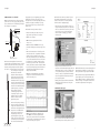
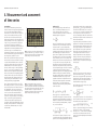
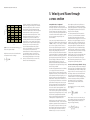
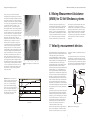
Velocity measurements
Guide and theory
Guide and theory
Quick guide
Velocity measurements in mixer
applications
1. Quick guide
Abstract
Velocity measurements in mixed tanks provide
information to both user and mixer supplier about the
performance of mixer installations. As measurements
can be carried out and evaluated in very different
ways, a standardised way of acquiring, evaluating and
reporting the velocity data is needed. A method for
measuring velocity in tanks of the circulation channel
type is described. The same principles hold in circular
tanks with horizontal bulk flow.
This guide assumes the user to be familiar with the
practical handling of the measurement equipment and
the ITT Flygt PC application “Mixing Measurement
Assistance” (MMA). The details of each are given in the
respective manuals [1, 2].
entities across a section is made with high accuracy
using the Gauss-Legendre Quadrature Scheme (GLQS).
Velocity measurements can be made efficiently with
an Acoustic Doppler Velocimeter (ADV) connected to a
computer for data storage. Other equipment, such as
an electromagnetic sensor, may be used but will yield
less precise results.
A computer program developed by ITT Flygt facilitates
the velocity measurement process and the evaluation
and presentation of the results. A suggested velocity
guarantee text is provided at the end.
The influence of the required accuracy on the
measurement time and the number of measurements
is addressed. Evaluation of average velocity and other
A. Preparatory work
This part may be possible to complete before visiting
the site, if enough information is at hand. If dimensions etc. must be collected on site, most of the data
is easily entered directly into the MMA program.
Supplementary input, such as a sketch, may be added
at any later time.
2 The location of one or several MXS is defined
according to practicability (access) and the guidelines
in Sec. 3 regarding clearance to flow disturbances.
A simple draw utility in MMA (Tank overview) may be
used to produce a clear sketch of the tank, the
situation, etc.
Table of contents
1. Quick guide
3
A. Preparatory work
3
B. Measurement – on site work
4
C. Evaluation and report
5
2. Introduction
6
3. Measurement cross section
and grid selection recommendations
7
4. Measurement and assessment of time series
8
4.1 Procedure
8
4.2 Theory
9
5. Velocity and fluxes through a cross section
1 Site/tank/mixer/aeration data is collected and entered
into MMA. MMA works with only one measurement
cross section (MXS) per report, but there is an edit
facility to generate several similar reports. Note that
several measured entities, such as velocity and
suspended solids concentration, can be collected in the
same report if they are measured at the same points.
11
5.1 Required values – background
11
5.2 Cross section average evaluation – theory
11
6. Mixing Measurement Assistance (MMA)
for 32-bit Windows systems
13
7. Velocity measuring devices
13
8. List of symbols and abbreviations
14
9. References
14
10. Velocity guarantee text
15
3 The MXS grid is defined in MMA. The default
given by the program is a Gauss-Legendre Quadrature
Scheme. Typically 5 x 5 points is recommended. If, on
site for instance, practical limitations make it necessary,
the grid can easily be redefined. A printout of the
measurement locations is convenient to bring to the
measurement site.
2
3
Quick guide
Quick guide
B. Measurement – on site work
4 Mark the horizontal positions of the measurement
points at the cross section, e.g. by putting tape on the
fence or tank wall etc. This facilitates the positioning of
the rod system, cf. item 6 below.
The uppermost (or second uppermost) pipe is always
held/fixed (it is also fixed to the rod by a screw).
The length scale on the rods helps keeping track of the
centimetres. The pipes are numbered, so by using
them in correct order, it is easy to keep track of the
metres as well.
7 The Nortek ADV may be started as follows:
Power supply
7I Connect the ADV power cable to the power
supply and the signal cable to the computer.
8 If ADV time series data are recorded to file, assess
the required measurement time for each point as
follows. If a time series is not recorded, 2 minutes
should be used for sampling/averaging.
8I Record a long series, preferably 10 minutes, of a
velocity measurement in a point close to the surface
and close to the wall. If the usual 5 x 5 grid is used,
select the point 51 or 55 for this measurement,
and save the data accordingly, e.g. in the file
site-mxs-51.adv.
7II Turn on the computer.
Other Probe
Velocity Probe
7III Run the ADV program (double-click the
“Vector” icon.)
7IV Fill in the relevant data. NB! This is the only
place where sampling rate and velocity range can be
set.
16 cm
Velocity Sampling Volume
5 The measurement equipment is mounted and
started according to the equipment manual, cf. item 7
below. First note that if more than one entity is to be
measured, consider putting several probes together.
For instance, a Solids Suspension probe can be taped
onto the body of a velocity probe.
Make sure there is minimum
interference between the probes.
(E.g. the suspension probe should
not disturb flow that goes into the
measurement volume of the velocity
probe.) This unfortunately affects the
accuracy of the cross section average
calculation of the additional quantity
(Solids Suspension), since the very
same horizontal and vertical
coordinates typically will not be
covered by this probe. It is recommended to keep this coordinate
deviation as small as to within
approximately 0.35 m.
6 The rods of the probe positioning
system are joined to a length which
corresponds to the distance from the
tank bottom to the height where the
rod system is to be held/fixed. The
velocity probe is mounted on the
first (lowest) pipe of the probe
positioning system. The pipe is put
to slide on the rods. Pipes are joined
to enable the probe to slide down to
the correct measurement depths.
7V To save the measurement in a data file, enter its
name at “Record To File”. As explained in the MMA
manual, the file name should be of the type sitemxs-11.adv, site-mxs-21.adv etc, for instance Grums1-11.adv. The numerals denote the row and column
in which the point is situated, counted from lower
left. All files, e.g. site-mxs-11.adv – site-mxs-55.adv
must be present before automatic reading into MMA
for processing and reporting. (If the measurement is
made with manual reading of data, this may be
directly entered into MMA.)
7VI The ADV “Probe Adjustment for boundaries”
will appear. To start the measurements, press the
”Start Disc Recording” icon.
8II Open this file from within the “Time Series
Assessment” menu in MMA (which appears after the
administrative menus for a case). For suitable values
of the confidence level (95 %) and the confidence
interval (±1 cm/sec), the required minimum sample
rate and the required total measurement time per
point are given by MMA.
10 All administrative data, the measurement grid, and
the resulting data, including cross section averages,
will be presented in the report printout from MMA.
11 The result data may be exported from MMA to an
external .fmp file, which can be shared with others
who use MMA. For instance, a global measurement
database is built up of all .fmp files e-mailed to staff
at the Public Utility Treatment at ITT Flygt HQ.
8III Using the sampling rate and measurement time
obtained in 8ii, measure at the rest of the points
(cf. item 7iv) above.
C. Evaluation and report
7VII Real time data will then be displayed on the
screen. NB! If no file name was specified under
“Record To File”, the data will not be saved and will
be unrecoverable. The measurement stops when the
”Stop Disc Recording” icon is pressed.
4
9 Enter the measured data into MMA either manually
or automatically from the .adv files, and save the case.
5
Quick guide
Quick guide
B. Measurement – on site work
4 Mark the horizontal positions of the measurement
points at the cross section, e.g. by putting tape on the
fence or tank wall etc. This facilitates the positioning of
the rod system, cf. item 6 below.
The uppermost (or second uppermost) pipe is always
held/fixed (it is also fixed to the rod by a screw).
The length scale on the rods helps keeping track of the
centimetres. The pipes are numbered, so by using
them in correct order, it is easy to keep track of the
metres as well.
7 The Nortek ADV may be started as follows:
Power supply
7I Connect the ADV power cable to the power
supply and the signal cable to the computer.
8 If ADV time series data are recorded to file, assess
the required measurement time for each point as
follows. If a time series is not recorded, 2 minutes
should be used for sampling/averaging.
8I Record a long series, preferably 10 minutes, of a
velocity measurement in a point close to the surface
and close to the wall. If the usual 5 x 5 grid is used,
select the point 51 or 55 for this measurement,
and save the data accordingly, e.g. in the file
site-mxs-51.adv.
7II Turn on the computer.
Other Probe
Velocity Probe
7III Run the ADV program (double-click the
“Vector” icon.)
7IV Fill in the relevant data. NB! This is the only
place where sampling rate and velocity range can be
set.
16 cm
Velocity Sampling Volume
5 The measurement equipment is mounted and
started according to the equipment manual, cf. item 7
below. First note that if more than one entity is to be
measured, consider putting several probes together.
For instance, a Solids Suspension probe can be taped
onto the body of a velocity probe.
Make sure there is minimum
interference between the probes.
(E.g. the suspension probe should
not disturb flow that goes into the
measurement volume of the velocity
probe.) This unfortunately affects the
accuracy of the cross section average
calculation of the additional quantity
(Solids Suspension), since the very
same horizontal and vertical
coordinates typically will not be
covered by this probe. It is recommended to keep this coordinate
deviation as small as to within
approximately 0.35 m.
6 The rods of the probe positioning
system are joined to a length which
corresponds to the distance from the
tank bottom to the height where the
rod system is to be held/fixed. The
velocity probe is mounted on the
first (lowest) pipe of the probe
positioning system. The pipe is put
to slide on the rods. Pipes are joined
to enable the probe to slide down to
the correct measurement depths.
7V To save the measurement in a data file, enter its
name at “Record To File”. As explained in the MMA
manual, the file name should be of the type sitemxs-11.adv, site-mxs-21.adv etc, for instance Grums1-11.adv. The numerals denote the row and column
in which the point is situated, counted from lower
left. All files, e.g. site-mxs-11.adv – site-mxs-55.adv
must be present before automatic reading into MMA
for processing and reporting. (If the measurement is
made with manual reading of data, this may be
directly entered into MMA.)
7VI The ADV “Probe Adjustment for boundaries”
will appear. To start the measurements, press the
”Start Disc Recording” icon.
8II Open this file from within the “Time Series
Assessment” menu in MMA (which appears after the
administrative menus for a case). For suitable values
of the confidence level (95 %) and the confidence
interval (±1 cm/sec), the required minimum sample
rate and the required total measurement time per
point are given by MMA.
10 All administrative data, the measurement grid, and
the resulting data, including cross section averages,
will be presented in the report printout from MMA.
11 The result data may be exported from MMA to an
external .fmp file, which can be shared with others
who use MMA. For instance, a global measurement
database is built up of all .fmp files e-mailed to staff
at the Public Utility Treatment at ITT Flygt HQ.
8III Using the sampling rate and measurement time
obtained in 8ii, measure at the rest of the points
(cf. item 7iv) above.
C. Evaluation and report
7VII Real time data will then be displayed on the
screen. NB! If no file name was specified under
“Record To File”, the data will not be saved and will
be unrecoverable. The measurement stops when the
”Stop Disc Recording” icon is pressed.
4
9 Enter the measured data into MMA either manually
or automatically from the .adv files, and save the case.
5
Introduction
Measurement cross section and grid selection recommendations
3. Measurement cross section and
grid selection recommendations
2. Introduction
ITT Flygt has developed a standardised method for
measurements and evaluation of velocity for
circulation channels, where the flow resembles free
surface channel flow, and for cylindrical tanks (tanks
of types 1 and 2). Similar standards for the remaining
tank type are under consideration. In cylindrical and
rectangular tanks the influence of secondary currents
and hydrodynamic instabilities are more dominating
than for channel type tanks, which means that
accurate velocity measurements in these cases requires
more planning and will be more time consuming.
The ITT Flygt method comprises recommendations for
selecting measuring points as well as for the way in
which measured data can be reduced into a few key
parameters. It also sets the format for documentation
to ensure uniformity of the result presentation.
Velocity measurements in mixed tanks provide
information about the installed mixer capacity and
how well it is used for mixing purposes. Velocity
and related quantities, e.g. turbulence intensity, are
parameters that link the mixer to the mixing and
process results. Moreover, flow velocity is often the
simplest visible parameter to use in order to judge the
performance of a mixer installation. To the authors'
knowledge, there are no standards developed for
velocity measurements in mixed tanks nor are there
any standards for how to evaluate the results of such
velocity measurements. It is therefore desirable to
establish a standardised method for performing and
evaluating velocity measurements in mixed tanks.
The large variety of possible tank shapes motivates a
division into three main types of tanks. These are:
weight to the interior points to ensure an accurate
evaluation of the cross section average. This is further
discussed in Sec. 5.2.
When the flow is of the open channel type, i.e. there
exists a dominant flow direction parallel to the side
walls of the tank, velocity measurements shall be
carried out in at least 25 points in at least one plane,
perpendicular to the main flow direction (i.e. perpendicular to the side walls). In circular tanks with an
ordered circulating bulk flow along the curved wall,
the same ideas hold. The MXS then extends from the
wall to the tank centre. The MXS planes should be
located in sections of the conduit where:
Because of the idealised property of the liquid surface
as a symmetry surface, the vertical distribution of
points is rather obtained by imagining a twice as high
channel with a confining ceiling at the top, and e.g.
10 points used for the double depth. Of course, only
5 of these occur in the real situation.
1. The cross section area is constant.
2. The flow is as developed as possible, which means
that the MXS shall be preceded by a straight
stretch, which is as long as possible. In circular
channels/tanks, no such stretch is available.
3. The MXS is as far as possible downstream from
flow disturbing objects such as bends, pillars,
mixers or others. A minimum distance should also
be kept upstream of such objects, to ensure that
the influence of these on the flow profile at the
MXS is negligible.
1. circulation channels: annular tanks, racetracks or
similar with a dominating channel flow
2. circular (cylindrical) tanks
3. rectangular tanks.
x
x
x
x
x
x
x
x
x
x
x
x
x
x
x
x
x
x
x
x
x
x
x
x
A sufficient number of points in both the horizontal
and vertical direction of the cross section should be
selected to ensure a reliable cross section average
evaluation. A minimum of 5 x 5 points is generally
recommended. The actual distribution of the points
in the section is determined according to a GaussLegendre Quadrature Scheme (GLQS) [3]. With 5 x 5
points, the locations in the cross section at which
measurements shall be made are shown in Fig. 1 and
Table 1. If the practical limitations (concerning access
etc.) to the point locations interfere with these
recommendations, slight modifications are possible to
make. In MMA, whole rows and columns can be
moved, with a subsequent revision of the corresponding
weights for maximum possible accuracy.
Figure 1 Cross section of a racetrack channel. Note that
the points of measurements are unevenly distributed for
best quality of evaluation.
ξi / W
αi
ηj / H
βj
0.047
0.231
0.5
0.769
0.953
0.1185
0.2393
0.2844
0.2393
0.1185
0.026
0.135
0.321
0.567
0.851
0.0667
0.1494
0.2191
0.2693
0.2955
Table 1 The positions and corresponding weights
recommended for maximum cross section average accuracy.
ξi is the ith position in the horizontal direction and αi is
the corresponding weight. W is the width of the cross
section. Similarly, ηj, βj, and H describe the set up in the
vertical direction.
It can be noted that the points are more densely
distributed along the channel sides and bottom, than
in the interior. However, the GLQS also assigns higher
6
x
7
Measurement and assessment of time series
Measurement and assessment of time series
4. Measurement and assessment
of time series
4.1 Procedure
The velocity in a measurement point varies from
moment to moment in a way that usually justifies the
use of basic statistic and probabilistic methods for
characterisation of the data. With an ADV probe, the
velocity can be recorded several times per second.
The whole series of velocities measured in a point
during some time interval is called a time series of the
velocity. An example of such a series, or signal, is shown
in Fig. 2. It is very common that if the velocity data
are collected in a histogram, the distribution of
velocities takes on the Gaussian form characteristic for
independent data stochastically distributed around a
mean value. In Fig. 3, such a distribution from a
measurement in Denmark is shown. The average value
and the standard deviation (σ) provide a description of
the average velocity conditions in a point.
4.2 Theory [4]
The natural way of treating a data series like the
above is to calculate the arithmetic mean of all
velocity observations (the sum of all velocity
observations divided by the number of observations.)
Mathematically this is expressed as:
40
30
Velocity (cm/s)
20
10
0
interval given by equation (4.2). For example, with P
equal to say 95%, t5% (f = 6500) (f taken from Fig. 2)
is found from a statistical table to be 1.96. Hence in
19 cases out of 20 (= 95%) the true expectation value
can be expected to be found in the interval (-5.01;
-4.51) cm/s. Generally, the width of the interval can be
reduced by increasing the number of observations and
thus the measurement time.
-10
(4.1)
-20
-30
-40
-50
200
400
600
800
1000
1200
1400
1600
Time (s)
Figure 2 Velocity at a point in the longitudinal direction of
a circulation ditch 180 m long, 5 m deep and 7 m wide in a
sewage treatment plant in Austria. 6500 observations were
obtained during a time period of 1300 seconds.
When a time series exhibits this behaviour, one expects
that an increase of the data set will make it converge
to a perfect Gaussian distribution with a certain true
average value, the expectation value, and with a true
standard deviation. It is reasonable to require of a
time series, that its average to a certain probability P
(say 0.97 = 97%) is at most a number I (say 1 cm/s)
different from the true expectation value. By stating
the two values P and I, the correspondingly required
number of data in a time series can be inferred, if a
relatively long time series is already present. The procedure for doing this is described below. It is automatically performed by the program MMA.
500
450
400
# observations
350
300
2
250
200
150
100
50
0
0
3
6
9
12
15
18
21
24
27
30
33
36
39
42
45
48
51
54
57
60
Velocity(cm/s)
There is, however, another restriction to put on the
data sampling. If the data in a point are recorded too
often, the velocity does not have time to change to a
new “independent” value. Hence if two data are
recorded within a very short interval, they may only
count as one in the above mentioned statistical
analysis. If for instance the velocity is periodic with
a period of 1 minute, measuring 1000 values during
totally 1 second will not yield a representative set
of data. The time needed to elapse between two
recordings is called the autocorrelation time (or macro
time scale), and the procedure for calculating it given
a test time series, described below, is also incorporated into MMA.
Figure 3 Velocity distribution (bars) of a time series
obtained in a circular tank in a sewage treatment plant in
Denmark. 5 measurements were made every second (sample
rate 5 Hz) during 8 minutes. The average value is 35.2 cm/sec.
Two standard deviations (2 σ) equals the width of the
distribution at half maximum. With some 2400 values, the
Gaussian character (filled area) clearly emerges.
In a dynamic system like a mixed tank we also have a
requirement on a sufficiently long measurement time.
(If it is desired to perform a frequency analysis of the
velocity signal, the dynamics of the mixed tank also
puts a requirement on the longest acceptable time
between two consecutive measurements. In such a
case the Nyquist criterion states that one has to
sample the signal with at least twice the highest
frequency component of the signal.) The length of
the required measurement period is linked to the
relative uncertainty ε of the estimate of the average
velocity through
where U is the arithmetic mean, N is the number of
observations and ui is the momentary velocity. It can
be shown that this is a good, normally the best,
estimate of the true mathematical expectation of the
underlying stochastic variable. It is interesting to note
what would happen if we split the data series in
Figure 2 into two equally long series and calculated
the arithmetic mean for each of them. The arithmetic
mean of the whole series is -4.76 cm/s, whereas the
arithmetic mean of the first and second half series are
-5.61 cm/s and -3.90 cm/s respectively. This rather
large difference remains even though the number of
observations and the observation time of even the half
series are impractically large. This calls for a statement
of the interval in which the estimate of the real
mathematical expectation of the underlying probability
distribution is likely to be found with some beforehand given probability. With the assumption that the
individual measurements of the velocity u can be
regarded as observations of independent stochastic
variables with unknown expectation and standard
deviation values, it can be shown that the true
mathematical expectation with probability P will be
found in the interval
(4.4)
where T0 is the macro time scale of the system, T is
the total measurement time, Urms is the root mean
square of the velocity signal and U is again the time
averaged velocity signal. The relative uncertainty, ε , is
defined as the variance of the experimental mean
normalised with the average velocity.
Both the Macro time scale T0 and Urms can be found
from a velocity signal. First,
(4.2)
(4.5)
where t1-P(f) is the 1 - P percentile of Student’s
t-distribution with f degrees of freedom, and d is the
experimental variance defined below. The Student’s tdistribution is tabulated in most statistical handbooks,
and is automatically calculated by MMA. f is equal to
N - 1, and d is found from:
For large values of N, Urms ≈ σ. T0 can be found from
the autocorrelation function of the velocity signal. The
autocorrelation function Ruu is defined as:
(4.6)
where τ is a separation variable; u(t) is the momentary
velocity at time t, and u(t+τ) is the momentary
velocity at time t + τ. Overbar means time averaging.
In words, the autocorrelation function is the time
average of the signal multiplied by itself but shifted a
time interval τ.
(4.3)
For the time series in Figure 2, d equals 0.13 cm/s.
In words this means that with a probability P the true
expectation of the underlying distribution is within the
8
9
Measurement and assessment of time series
Measurement and assessment of time series
4. Measurement and assessment
of time series
4.1 Procedure
The velocity in a measurement point varies from
moment to moment in a way that usually justifies the
use of basic statistic and probabilistic methods for
characterisation of the data. With an ADV probe, the
velocity can be recorded several times per second.
The whole series of velocities measured in a point
during some time interval is called a time series of the
velocity. An example of such a series, or signal, is shown
in Fig. 2. It is very common that if the velocity data
are collected in a histogram, the distribution of
velocities takes on the Gaussian form characteristic for
independent data stochastically distributed around a
mean value. In Fig. 3, such a distribution from a
measurement in Denmark is shown. The average value
and the standard deviation (σ) provide a description of
the average velocity conditions in a point.
4.2 Theory [4]
The natural way of treating a data series like the
above is to calculate the arithmetic mean of all
velocity observations (the sum of all velocity
observations divided by the number of observations.)
Mathematically this is expressed as:
40
30
Velocity (cm/s)
20
10
0
interval given by equation (4.2). For example, with P
equal to say 95%, t5% (f = 6500) (f taken from Fig. 2)
is found from a statistical table to be 1.96. Hence in
19 cases out of 20 (= 95%) the true expectation value
can be expected to be found in the interval (-5.01;
-4.51) cm/s. Generally, the width of the interval can be
reduced by increasing the number of observations and
thus the measurement time.
-10
(4.1)
-20
-30
-40
-50
200
400
600
800
1000
1200
1400
1600
Time (s)
Figure 2 Velocity at a point in the longitudinal direction of
a circulation ditch 180 m long, 5 m deep and 7 m wide in a
sewage treatment plant in Austria. 6500 observations were
obtained during a time period of 1300 seconds.
When a time series exhibits this behaviour, one expects
that an increase of the data set will make it converge
to a perfect Gaussian distribution with a certain true
average value, the expectation value, and with a true
standard deviation. It is reasonable to require of a
time series, that its average to a certain probability P
(say 0.97 = 97%) is at most a number I (say 1 cm/s)
different from the true expectation value. By stating
the two values P and I, the correspondingly required
number of data in a time series can be inferred, if a
relatively long time series is already present. The procedure for doing this is described below. It is automatically performed by the program MMA.
500
450
400
# observations
350
300
2
250
200
150
100
50
0
0
3
6
9
12
15
18
21
24
27
30
33
36
39
42
45
48
51
54
57
60
Velocity(cm/s)
There is, however, another restriction to put on the
data sampling. If the data in a point are recorded too
often, the velocity does not have time to change to a
new “independent” value. Hence if two data are
recorded within a very short interval, they may only
count as one in the above mentioned statistical
analysis. If for instance the velocity is periodic with
a period of 1 minute, measuring 1000 values during
totally 1 second will not yield a representative set
of data. The time needed to elapse between two
recordings is called the autocorrelation time (or macro
time scale), and the procedure for calculating it given
a test time series, described below, is also incorporated into MMA.
Figure 3 Velocity distribution (bars) of a time series
obtained in a circular tank in a sewage treatment plant in
Denmark. 5 measurements were made every second (sample
rate 5 Hz) during 8 minutes. The average value is 35.2 cm/sec.
Two standard deviations (2 σ) equals the width of the
distribution at half maximum. With some 2400 values, the
Gaussian character (filled area) clearly emerges.
In a dynamic system like a mixed tank we also have a
requirement on a sufficiently long measurement time.
(If it is desired to perform a frequency analysis of the
velocity signal, the dynamics of the mixed tank also
puts a requirement on the longest acceptable time
between two consecutive measurements. In such a
case the Nyquist criterion states that one has to
sample the signal with at least twice the highest
frequency component of the signal.) The length of
the required measurement period is linked to the
relative uncertainty ε of the estimate of the average
velocity through
where U is the arithmetic mean, N is the number of
observations and ui is the momentary velocity. It can
be shown that this is a good, normally the best,
estimate of the true mathematical expectation of the
underlying stochastic variable. It is interesting to note
what would happen if we split the data series in
Figure 2 into two equally long series and calculated
the arithmetic mean for each of them. The arithmetic
mean of the whole series is -4.76 cm/s, whereas the
arithmetic mean of the first and second half series are
-5.61 cm/s and -3.90 cm/s respectively. This rather
large difference remains even though the number of
observations and the observation time of even the half
series are impractically large. This calls for a statement
of the interval in which the estimate of the real
mathematical expectation of the underlying probability
distribution is likely to be found with some beforehand given probability. With the assumption that the
individual measurements of the velocity u can be
regarded as observations of independent stochastic
variables with unknown expectation and standard
deviation values, it can be shown that the true
mathematical expectation with probability P will be
found in the interval
(4.4)
where T0 is the macro time scale of the system, T is
the total measurement time, Urms is the root mean
square of the velocity signal and U is again the time
averaged velocity signal. The relative uncertainty, ε , is
defined as the variance of the experimental mean
normalised with the average velocity.
Both the Macro time scale T0 and Urms can be found
from a velocity signal. First,
(4.2)
(4.5)
where t1-P(f) is the 1 - P percentile of Student’s
t-distribution with f degrees of freedom, and d is the
experimental variance defined below. The Student’s tdistribution is tabulated in most statistical handbooks,
and is automatically calculated by MMA. f is equal to
N - 1, and d is found from:
For large values of N, Urms ≈ σ. T0 can be found from
the autocorrelation function of the velocity signal. The
autocorrelation function Ruu is defined as:
(4.6)
where τ is a separation variable; u(t) is the momentary
velocity at time t, and u(t+τ) is the momentary
velocity at time t + τ. Overbar means time averaging.
In words, the autocorrelation function is the time
average of the signal multiplied by itself but shifted a
time interval τ.
(4.3)
For the time series in Figure 2, d equals 0.13 cm/s.
In words this means that with a probability P the true
expectation of the underlying distribution is within the
8
9
Measurement and assessment of time series
Velocity and fluxes through a cross section
5. Velocity and fluxes through
a cross section
(In practice, the integral is often evaluated from 0 to
the first zero of Ruu, which is likely to be conservative
for the present purposes.) T0, which is a measure of
the longest time scales in the turbulent flow field,
can be used in Equation (4.4) to find out the required
measurement time T in order to get the average
velocity with a relative uncertainty less than ε. For the
example above the Macro time scale is about 10 s.
Using Equation (4.4), it becomes evident that an
uncertainty (defined as the variance of the experimental
mean) less than 0.13 cm/s, requires over 40 hours of
measurement, which is quite an unrealistic operation.
If, however, one can accept an uncertainty of 2.0
cm/s, the required measurement time, instead, is
about 10 min, still prohibitive if one considers that
some 30 points are to be measured in one
measurement section. While the example given here
is, as stated above, extreme, it serves well as an
illustration of the precautions that have to be taken
when a seemingly simple thing such as an average
velocity is to be measured. In more common cases,
the macro time is substantially shorter.
1
0.8
Ruu (τ)
0.6
0.4
0.2
0
-0.2
-0.4
0
200
400
600
800
τ (s)
Figure 4 A plot of the autocorrelation function Ruu(τ) as a
function of the separation variable τ.
Finally the macro time scale can be found from the
autocorrelation function according to:
(4.7)
bottom might be specified. Such specifications are
tricky to deal with, as local variations will always be
present, although the mean velocity may be very high.
Literally fulfilling this requirement leads to excessive
sizing for the actual mixing duty.
5.1 Required values – background
In many mixer applications a certain value of the
flow velocity is specified. Since the velocity varies from
point to point and from moment to moment, a time
and space average value is the simplest to specify. In
some cases, a true net transport of liquid from A to B,
or around a circulation ditch is required at a certain
rate. Then the average transport velocity is the
obvious candidate.
Once velocity measurements have been made in a
cross section, one can derive kinematic information
other than just the average velocity. This includes
momentum and kinetic energy flux across the section.
When there is a thorough investigation of the flow
conditions, these entities can shed light on the total
situation. Normally, though, they are of little interest.
An exception might be the momentum flux, which
actually contains the value of the bulk flow velocity
which mixer sizing is really based on. This may differ
by some amount from the value arrived at according
to the procedure adopted in this handbook.
Therefore, when a velocity is to be guaranteed, rather
than the mixing duty this velocity is supposed to
effect, special care should be taken. In ITT Flygt’s
Mixer Dimensioning System, MiDS, there is a function
for sizing mixers to guaranteeing velocities.
Often, some velocity is stated with reference to the
mixing duty of sediment avoidance and related results.
In WWTPs, a value of 0.3 m/s (1 ft/sec), or sometimes
up to 0.35 m/s or higher, or down to 0.22 m/s or
even lower is specified. These figures are based on
experience and initially emerged from an analogy with
sewage or slurry pumping. The reasons for the
variation of this value are the different characteristics
of waste water, differences in pretreatment in WWTPs,
differences in conditions in the tank (e.g. presence of
pipes along the bottom, which hinders the flow and
promotes settling), and differences in additional
mixing requirements that may or may not be
expressed. The bulk flow velocity as defined below is
actually required to have larger values in deeper tanks,
but this is rarely considered.
5.2 Cross section average evaluation – theory
The natural procedure for time and space averaging of
the velocity consists of first finding the time average in
each measurement point and then calculating a space
average – in this case a cross section average – of the
time averages. If there were a device that measured
the velocity in all points simultaneously, then one
could have done the cross section averaging for every
instant of measurement, and finally calculated the
time average of these cross section averages.
There is no handy such device available for the
moment, though.
Since this velocity requirement refers to local conditions,
i.e. in a major part of the tank or channel, the
direction of the flow is of minor importance, and the
magnitude of the velocity can be considered to be the
relevant parameter for mixing. Still, typically one or a
few main circulation loops are generated with submersible mixers. Therefore, there is an indication of a
way of selecting a measurement cross section where a
representative tank average value of the velocity can
be found. The net transport velocity (responsible for
the volumetric flux) across such a section is of the
same order as the total velocity magnitude – hence
measuring only the velocity component perpendicular
to the cross section gives a good hint of the prevailing
average velocity. The average velocity across a correctly
selected section is generally termed the bulk flow
velocity – and mixer sizing and positioning is most
commonly based on a required value of this.
The average velocity in a cross section, denoted by
<U>, is given by
(5.1)
where A denotes cross section area and x and y are
the coordinates in the plane of measurement. Using
the Gauss Legendre Quadrature Scheme [3] the
integral can be approximated by
Rarely does one encounter specifications for other
flow variables than the velocity – even in heat transfer
applications, requirements are often translated into a
velocity. However, it may be that the velocity is sometimes required to attain a minimum (or maximum)
value at certain points of the tank. For instance, a
minimum velocity of 0.15 m/s at 10 cm from the
10
(5.2)
11
Velocity and fluxes through a cross section
MMA for 32-bit Windows systems, Velocity measurement devices
6. Mixing Measurement Assistance
(MMA) for 32-bit Windows systems
where ξi and ηj are the vertical and horizontal
measurement positions respectively, and αi and βj are
the weight factors resulting from the GLQS mentioned
above. (Here, 5 locations in each direction have been
assumed. A conventional factor 1/4 has been absorbed
into αi and βj.) The same approximation of the integral
can be applied to find area averages of other
quantities, e.g. <U2>. The reason for using the
Gauss-Legendre method is that it closely approximates
the integral of a not too chaotic function better than
most other methods. It does not however, improve the
accuracy of the function U (as opposed to the value
<U>) or the values used to represent it. To illustrate
the exactness of the method we consider two
examples where the flow through a channel is to be
determined. (Only one component of velocity is
measured.) The velocity profiles are given by the
contour diagrams in Figure 5a, generated by MMA.
In the second cross section, there is flow reversal,
which typically occurs close to mixers and just after
racetrack bends. In Figure 5b, the application of GLQS
and simple averaging with evenly distributed points is
shown to produce differences in accuracy. Note that
the number of measurement points is equal to the
square of the number on the horizontal axis. For a
very simple flow profile, there seems to be little or no
gain in using the GLQS, but the stability with which
this method approaches the true value as the number
of points increases, is extremely valuable. In addition,
as soon as a profile with more structure occurs, the
gain is dramatic. As realistic profiles always contain
some structure, it is easy to realise the benefit of
always using a GLQS.
Figure 5a Contour diagrams of two ficticious velocity
profiles.
0.3
0.37
0.1
m/s
0.36
0.35
0.34
-0.1
0.33
0.32
-0.3
2
The average velocity (and average dry solids content,
or temperature, pH or whatever is measured) is
calculated, and a contour diagram of each measured
quantity is produced. All this is collected in a report,
where the measurement grid and the corresponding
weights (cf. Table 1) also are shown. To each MXS
corresponds one report, regardless of what quantities
are measured. There is an extensive manual to the
program [2].
7. Velocity measurement devices
0.38
m/s
Figure 5b Approach to true cross section
average as the number of columns and rows
increases. Diamonds denote GLQS values
(from 2 x 2 to 5 x 5 points) and squares
denote even point distribution averaging
(from 3 x 3 to 10 x 10 points). Dotted lines
refer to the left scale (the upper profile in
Figure 5a), and solid lines to the right scale
(the lower profile in Figure 5a). Lines with
no symbols define the true values.
The theories and procedures outlined above for a
sound measurement and evaluation of the bulk flow
velocity comprise an extensive mathematical and
practical apparatus. As is evident from the Quick
guide (Sec. 1), much of the mathematical work has
been automatised in the MMA program. In addition,
a summary of administrative data such as time and
place of measurement, geometry of channel/tank,
and other conditions that are of interest, is made.
3
4
5
6
#rows=#columns
7
8
9
10
may be made available to any subsidiary company of
ITT Flygt.
Any instrument made for velocity measurements can in
theory be used for the kind of measurements discussed
in this paper. However, practical restrictions like
accuracy, handling principles, sensitivity to clogging,
measurement output format etc. restrict the variety of
usable instruments. In real life mixing applications the
most suitable instruments are Accoustic Doppler
Velocimeter (ADV) systems or electromagnetic velocity
measurement instruments. The Acoustic Doppler
Velocimeter system used by ITT Flygt is manufactured by
Nortek AS, Norway [1]. It is a handy and easy to use
tool for velocity measurements in both laboratory and
real applications. It can determine the complete velocity
vector (i.e. the velocity in all three mutually orthogonal
directions), in one point at a time, a feature that few
other velocity measuring systems can offer. The current
system can measure and store up to 64 measurements
per second, which means that some characteristics of
the turbulence can be determined or at least estimated.
To the authors knowledge these characteristics make the
ADV system the best choice for velocity measurements
in mixed tanks.
The output from the ADV system is one data file per
measuring point, containing a time series of velocity
readings. Software to extract useful numbers from the
time series in the ADV files is available on the computer.
For a discussion of the required length and number of
data points in the time series, refer to Sec. 4 above.
Power supply
Other Probe
The principle of operation is that the instrument emits
ultrasonic beams that are reflected by small particles
entrained in the liquid. The reflected sonic beams are
picked up by a receiver. The frequency of the reflected
sound is shifted in proportion to the velocity of the
reflecting particle. The frequency change between
emitted and received sound is determined by the
electronics in the instrument and reported to a
computer that handles the data storage.
16 cm
Velocity Sampling Volume
Figure 6 The ADV measuring system.
The Nortek ADV system used by ITT Flygt consists of a
probe, a power supply, and a computer with driver
software to control the system, cf. Fig 6. The system
12
Velocity Probe
13
List of symbols and abbreviations, References
Velocity guarantee text
8. List of symbols and abbreviations
d
variance of a time series,
1/2
equal to σ / N
f
N – 1; number of degrees of
freedom in Student’s t-distribution
t, τ
time
t1-P(f)
Student’s t-distribution
ui, u(t)
momentary (measured) velocity value
x; y
coordinates in a MXS
A
cross section area
ADV
Acoustic Doppler Velocimeter
MMA
Mixing Measurement Assistance
(ITT Flygt software)
GLQS
P
Gauss-Legendre quadrature scheme
for approximating an integral with
a finite sum
probability that the average of a
measured time series lies within a certain
interval (I) around the expectation value
of the underlying stochastic variable
(“true value”)
Ruu(τ)
autocorrelation function of time series
T0
autocorrelation (or macro) time scale
of a time series
U
average value of a series of velocity
values in a point
<U>
cross section average of U
Urms
”root mean square” of velocity signal,
close to σ for large N
W
width of MXS
WWTP
waste water treatment plant
αi ; βj
weights defined for cross section
averaging using GLQS, cf. Eq. (5.2)
H
liquid depth, i.e. height of MXS
I
cf. P below
ε
relative uncertainty, cf. Eq. (4.4)
MXS
measurement cross section
ξ i ; ηj
N
number of measured values in
a time series
measurement point positions defined for
cross section averaging using GLQS, cf.
Eq. (5.2), Fig. 1 and Table 1.
σ
standard deviation of time series,
cf. Eq. (4.3)
10. Velocity guarantee text
3. The magnitude of the velocity is measured in
each point.
“It is generally known and accepted that mixer
generated flow in ditches and tanks in WWTPs is
turbulent. Therefore, the velocity may assume highly
varying values, and may even reverse, in a single point.
At physical boundaries, the velocity vanishes, although
it acts via a shear stress all the way to the boundary
(wall, bottom, ...). In view of these circumstances, it is
not reasonable to request a minimum velocity in a
whole volume or in a whole cross section. With regard
to mixing, an average, or bulk flow velocity in a cross
section is a reasonable entity to prescribe.
4. The sampling rate and the minimum total integration time to be used is assessed to achieve a
confidence interval of ± 0.01 m/s at a confidence
level of 95%. Typically some 2 minutes sampling at
minimum 5 Hz rate at each point is required.
5. The total error in the measured cross section
average is asserted to be ± 0.01 m/s ± the
inaccuracy of the velocity probe.
The bulk flow velocity is measured according to ITT
Flygt’s Velocity Measurement Guide, as briefly outlined
below:
ITT Flygt (name of subsidiary) guarantees that
the bulk flow velocity generated by the mixer in the
channel/tank under normal operating conditions
(e.g. those on which the mixer design was based), to
within the total error, is at least (fill in value) m/s.”
1. A measurement cross section across the bulk flow
is selected where the flow is developed and its
character is unaffected by flow disturbing objects
in the channel/tank.
2. A grid of measurement points, typically no less
than 5 x 5, is selected using the Gauss-Legendre
Quadrature Scheme. The scheme produces unevenly
spaced points and the corresponding weights
are unequal.
9. References
4. Cramér, H., Mathematical methods of statistics,
Princeton Mathematical Series 9, Almqvist &
Wiksells (USA, 1946); Blom, G. Sannolikhetsteori
och statistikteori med tillämpningar,
Studentlitteratur (Lund, 1970).
1. ADV Software Reference Manual, Nortek AS
(Vollen, Norway, January 2 1996); ADV Operation
Manual, Nortek AS (Vollen, Norway, January 2
1996).
2. User manual for MMA Mixing Measurement
Assistance, ITT Flygt AB (Solna, 2000).
Additional reading:
Johansson, A. V., & Alfredsson, P. H. (March 1988)
Experimentella metoder inom strömningsmekaniken.
Institutionen för Mekanik, KTH, Stockholm.
3. Handbook of mathematical functions, National
Bureau of Standards, Applied Mathematics Series
55 (November 1970); Korn G. A. & Korn T. M.,
Mathematical Handbook for Scientists and
Engineers, 2nd Ed., McGraw-Hill (New York, 1968).
14
15
ITT Flygt is the world’s leading manufacturer, supplier and innovator on the
submersible pump, mixer and aeration markets. With production facilities in
four continents our products are used everyday in wastewater treatment plants,
sewage systems, aqua-agriculture, the process industry and numerous other
applications. Our experience is utilised by engineers, planners and consultants to
ensure reliable and cost-effective use of our systems in all corners
of the world.
www.flygt.com
Velocity measurements.02.01.Eng.1M.01.02. © ITT Flygt AB 894140
ITT Flygt is represented in over 130 countries and has 37 sales companies
around the world.