Download User Guide to BayesMix

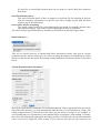
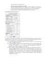
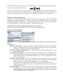
User Guide to BayesMix v.1.0
Kerry Gallagher, August 2009
[email protected]
Background
The BayesMixQt application allows us to infer the probability distribution of the number of
component distributions from a distribution of input ages (+ associated errors), under the
assumption of either Normal (Gaussian) or Skew-t distributions. Furthermore, we infer the
parameters defined each component distribution (such as the mean, standard deviation, left and
right skewness), and also the proportion of each individual component distribution contributing
to the total distribution. Each parameter has an uncertainty and these are characterized through
the 95% credible range.
The approach implemented uses Reversible Jump Markov chain Monte Carlo (RJMCMC), which is a iterative sampling strategy, allowing for the dimension of the model
parameter space to change (i.e. the number of component distributions and the parameters
associated with each component distribution). We use a Bayesian formulation, which requires
the specification of both prior distributions and proposal distributions. For the prior distributions,
these are generally set to default values, so the user does not need to specify the form. For the
proposal distributions, default values can be used, and adjusted according to the acceptance rate
of proposed parameter values. The acceptance rates are monitored during a run and output at the
end, allowing the user to update their values, interactively.
The results can be examined through a series of plots, and summary statistics
written to the screen (and, optionally to an output file).
The main reference for the methodology used in this application is
Jasra, A., Stephens, D.A. Gallagher, K. and Holmes, C.C., (2006) Analysis of
geochronological data with measurement error using Bayesian mixtures,
Mathematical Geology, 38(3), 269-300
(and there are references to various earlier papers in this one). An additional reference
describing the use of RJMCMC methods in Earth Science problems is
Gallagher, K. Charvin, K. Nielsen, S., Sambridge, M. and Stephenson, J. (2009)
Markov chin Monte Carlo (MCMC) sampling methods to determine optimal
models, odel resolution and model choice for Earth Science problems, Marine and
Petroleum Geology, 26, 525-535.
PLATFORMS
The computational engine in BayesMixQt is written in C/C++, and the Graphical User Interface
(GUI) is written in Qt. Currently, the application is configured to run on Macintosh (Intel
processor with Mac OS X 10.3 or higher), but in the future, our plan is to port it to run also under
Windows.
INSTALLATION
Having mounted the disk image, double click on the installation package and follow the
instructions. The install package will produce the application, BayesMixQT, and an example data
file, age_2.txt (these are synthetic data are sampled from 2 equally weighted normal distributions
- the input format for data files is 2 columns of age and error). In addition the two papers
mentioned above are included as pdf files.
Note the current version places 3 dynamic link library files for Qt (QtCore, QtGui, QtSvg) in the
directory /Library/Frameworks. You may need administrator permission to do this (you will be
prompted during the install process). Installing later versions of BayesMixQt should not require
reinstalling the library files.
RUNNING BAYESMIXQT
When you launch BayesMixQt, various menus will be loaded onto the system toolbar and a main
window will be shown, as below. On this window, a local toolbar with icons for copy, cut, etc is
loaded. This window is used for writing selected output during the running of the application.
Initially, some application specific messages are written (such as the limitations on the number of
data used).
There are 4 menus on the system toolbar :
BayesMixQT>
This is the system menu. It has the About BayesMixQt and the quit option at the bottom of the
menu.
File >
This is the menu to open and save files
Open
You will be prompted to enter a data file name. The data file format is a simple file with 2
columns of age and error. The 2 columns can be separated by spaces or tab. Once read,
the values and the total number of data read are written to the screen.
If a data file is successfully opened, then you can look at a crude radial plot, under the
Plot menu.
Save Run Summary file as
This saves the main details of the run output to a specified file for archiving if desired.
Note the summary information for specific runs can be simply copied from the main
window (this is described later).
Do not delete all files on quitting
This keeps various work files created during the run which are normally deleted when
you quit BayesMixQt. This can be useful for debugging if there are problems.
The last 5 recently opened data files are listed below this menu (not shown in figure here)
Run Parameters >
This lets us choose between a Normal and Skew distribution model, and specify various
parameters for the chosen model type, as well as selecting the number of components to collect
details on, and also has the option for running a model simulation. Each menu option is described
below.
Normal Distribution Run Parameters
Specify the input MCMC parameters for normal distributions. If the program has been previously
run in the same directory, we will automatically load the last set of run parameters, using a file
called normprevious.txt. If this file does not exist (you can delete or rename it, for example, to
avoid loading this set of parameters), some default values are assigned. After loading, or setting,
the values can subsequently changed in this dialog window. If desired, the current run parameters
can be saved to an output file (with a name of your choice) after the run (the current set of
parameters will be saved to normprevious.txt by default). If you have saved a previous set of run
parameters to a filename of your choice, you can read these in from the file using Load Previous
Parameters button. You will be prompted for a file name. You generally need to enter something
in one of the boxes to activate the OK button - you can just type the same value that is in the box.
Note all these parameters are checked that they have a valid value (e.g. positive). If the OK
button does not become activated it may be because one the parameters is not valid.
These input parameters are
(i)
Scale factor for data errors – this allows us to specify or search for a scaling factor
on the input errors. If you type a value into the Min box, the Max box will
automatically be set to the same value. In this case, we use this value to scale the
input errors. If you modify the Max value, then we use the range to search for a
scaling factor.
(ii)
Range for sigma (for distributions) – this allows us to specify a range (in terms of
minimum and maximum values) for the acceptable values of the standard
deviation (scale parameter) for the component distributions. This may arise given
the context of the problem being considered. For example, trying to distinguish
different eruption ages in a lava pile implies a different duration for an age
component than discrete episodes of continental crust formation. The default is
just a positive number.
(iii)
Proposal scales – this lets us set the proposal function scaling parameters for the
different parameters associated with each component. For normal distributions,
these are the mean (mu, or location parameter in statistics), inverse variance
(lambda = 1/sigma2, with sigma = standard deviation or scale parameter in
statistics), and the proportions of each component. We need select values for the
data resampling (which is a 2 stage process – a good rule of thumb is to use a
value of the second stage equal to about 0.2 of the first stage). Finally, if we
choose to seach for a scale factor on the data errors (see (i)), then we need to input
a proposal scale for this parameter also.
To decide a good value of these proposal parameters, we look at the acceptance values
for each parameter type after a run (these will be shown in the box to the right for each
parameter type). Typically a value between 0.3 and 0.6 is OK (again for the data
resampling we tune the parameters so that stage 2 has a value in this range). In general,
to increase the acceptance rate, we decrease the proposal scale, and to decrease the
acceptance rate, we increase the proposal scale.
(iv)
We need to specify the burn-in, post-burn-in and thinning parameters for the
MCMC chain. The burn-in allows for some exploratory sampling of the model
space during the early stages of the MCMC sampling. These samples are
discarded from those subsequently collected and used to infer the component
distribution parameters (i.e. the post-burnin samples). The total number of
iterations is then burn-in + post-burn-in. The thinning is just a factor used to
reduced the total number of samples collected (post-burn-in) and to reduce the
effect of correlation between successive samples (in general this is not a big issue
though, if enough post-burn-in samples have been used). For example, if burn-in
is 50000, post-burn-in is 120000 and thinning is 5, then we will run 170000
iterations, discard the 50000, keeping every 5th of the last 120000 (leading to
120000/5 = 24000 samples in total used to make the inference). The suitability of
the burn-in length can be assessed once the run is made by looking at the
likelihood chain (under the plots menu, as described later). Note that currently
there is a limitation on the number of samples collected, and this is specified in
the main window at start-up as below
This can be translated back to post-burn-in = 20000 * thinning. So if thinning =
10, the maximum post-burn-in = 200000. If you want more post-burn-in
iterations, increase the thinning accordingly (thinning = post-burn-in/20000).
Note the burn-in, post-burn-in and thinning all have to be integers.
Skew Distribution Run Parameters
As above but for skew distributions. The default parameter file from a previous run is
skewprevious.txt. Note there are more options for the skew distribution parameters and the
details are given in the Jasra et al. (2006) paper. In particular we can choose
(a) a prior distribution which favours light or heavy skew (prior 1 and 2 of Jasra et al
2006). The default is light skew.
(b) a relative weighting on negative skew, symmetrical and positive skew distributions (the
default is equal weighting = 1/3 = 33.33%). You can enter any positive number here
(but not as a fraction i.e. not 1/3), and they will be normalized to a total of 1,
maintaining the relative weighting you have input.
(c) either a uniform or Poisson distribution on the number of components (note that for a
Normal distribution model we always use a uniform distribution). The range for a
uniform distribution is set to a lower value of 1 and a maximum equal to either 50 or
the number of observed data which ever is the smallest). For a Poisson distribution, the
lower value is also 1, and the user needs to specify the mean value for the number of
components (an integer between 1 and the maximum number of data). The default
distribution is uniform.
(d) values for the proposal distribution on the skew parameters, nu and eta. The same value
is used for both parameters. The tuning of this value to achieve a suitable acceptance
rate follows the same strategy as for the other parameters described for the normal
distribution models.
(e) value for the truncation parameter if using prior 1, as described in Jasra et al (2006)
(note the default value is usually OK, and from experience, this value need not be
changed).
Select Number of components to monitor
We can select a specific number of components to monitor during a run for a more complete
output. Usually this will be done after at least one exploratory run to determine a reasonable set
of input parameters, and examination of the results. For example, having determined a reasonable
set of input parameters, we might want to output the results for the maximum posterior
probability model with N components. If a value is not selected before running the MCMC
sampler, then this option will be disabled. This value is limited to between 1 and the number of
data or 50 (which ever is less).
Run
Runs the models, showing a progress dialog box. Once the run is finished, a dialog box with the
input MCMC parameters and the acceptance rates for each parameter, as shown below for a
Normal distribution run.
It is recommended to examine the acceptance rates for the distribution parameters, e.g. mu,
lambda, pi, etc. These should be around 0.3 to 0.6 for acceptable sampling. For the data
resampling, don't worry too much about the value for stage 1.
If all is OK, then to activate the other plots in the Plot menu, just click on Cancel.
If you want to edit certain MCMC parameters, then you can do this. The button modify for rerun
will be activated. If you click this, then you can return to the Run option and rerun the MCMC
sampler.
If you want to save the current set of input parameters to a file, then click on the Save Current
Run Parameters button, and you will be prompted for the file name. This file can later be opened
from the Normal/Skew Distribution Run Parameters menu options. The OK button will be
activated after you have saved the file.
If you cancel the run, then you need to select again the model type (Normal or Skew) and run a
simulation again to active any plotting options.
Plot >
Once a run is successfully completed, all of the appropriate plot options will be enabled. These
are considered in turn below. All plots allow the position of the mouse to be monitored in local
co-ordinates. If you place the mouse in the plot window, and hold the select button down, you
will see cross-hairs marking the position, and the co-ordinates are written at the bottom left of the
plot.
Plots can be saved directly into SVG (scaled graphics format) which is compatible with many
standard graphics packages (well at least Adobe Illustrator), and/or printed directly. You can also
print to a pdf file if you prefer this to SVG format.
Radial plot
A crude radial plot of 1./error against (age-mean age)/error. With this plot all data are
transformed to have the same relative error (±2 = ±2 sigma). This is a useful graphical way to
quickly assess how many components we might expect. An average age for a given group of data
could be given by the slope of a regression line passing though a group of data and the origin.
See Galbraith, R. (1988). "Graphical display of estimates having differing standard errors".
Technometrics 30 (3), 271-281.
Examine Chain (Likelihood, Posterior, optionally Data Error Scaling, and Data Resampling
Chains).
Plots the log of the likelihood or the posterior against iteration (post-burn-in) (blue), as well as
the number of components (green) sampled at each iteration. This is a useful diagnostic for the
behaviour of the sampler. If you chose to infer a scaling parameter on the data errors, you can
also look at the value of this as a function of iteration. The post-burn-in sampling should look
pretty much like a white noise series, with no obvious trends in the blue curve.
The Data Resampling Chain plots the mean squared (error normalized) deviation between the
2
1 Ndata ⎛ x i − y i ⎞
observed (x) and sampled (y) values i.e.
⎟
∑ ⎜
Ndata i= 1 ⎝ αεi ⎠
where ε is the input error value, and α is the data error scaling factor for the current iteration. The
blue line is this value, and we also plot the ±1 std deviation about this value as a function of
iteration. On the y-axis, ±2 is effectively the 95% probability range about a zero deviation.
€
Number of components histogram
Summarises the probability distribution on k, the number of components. This is useful when
deciding how many components are valid. We want to select models using the value of k with
the highest probability. Typically, we would examine this plot after one or more exploratory
runs, and then choose a value for the number of components to monitor.
Data Scaling Error Factor histogram (if this option was selected)
Summarises the probability distribution on the data error scaling parameter.
Maximum Likelihood Model
Maximum Posterior Model
These allows series of plots to be examined for the Maximum Likelihood or Maximum Posterior
models.
The plots are
Model Joint Distribution - plots the predicted combined distribution for the selected model,
together with the estimate of the mean (location parameter mu) for each component.
The height of each line reflected the proportion (pi).
Individual Component Distributions - as above, but also plots the distribution for each
component separately.
Classification Probabilities - for each age, we plot the probability it can be assigned to each
component distribution. The data are shown as x. Note that the ages plotted here are
not the observed values, but rather the sampled ‘true’ values (y as opposed to x in the
Jasra et al 2005 paper).
Sampled v Observed ages - plots the relationship between the input observed and the
sampled ages (x and y in the paper of Jasra et al. 2005). The observed ages have the
input error plotted (±1 sigma). The straight line is a 1:1 relationship.
(note that if we are using this plot for the expected model, as described later, the
sampled ages have an error bar equal to ±1 standard deviation of the values sampled
during the MCMC run).
Summary Statistics – writes the numerical values summarizing the component distributions
and model run to the screen. These can be copied/cut/cleared from the screen using
the tool bar options on the main window (and the default key strokes such as cmd-C,
cmd-X should also work on a Macintosh).
An example of the screen output for a Skew Distribution model, maximum likelihood is
given below
========================================
/Users/kerry/projects/BayesMix/age_2.txt
Max. Likelihood Model Results
No of components = 8
Log Likelihood = 28.901264 Log Posterior = -37.415773
Component 1: : Mode = 324.01 Mu = 324.179 Sigma = 4.37508 Nu = 2.71592 Eta = 2.8183 Pi = 0.028602
Component 2: : Mode = 363.28 Mu = 367.079 Sigma = 3.82516 Nu = 4.70364 Eta = 8.43609 Pi = 0.078583
Component 3: : Mode = 396.5 Mu = 422.175 Sigma = 26.3069 Nu = 5.81068 Eta = 9.7933 Pi = 0.010663
Component 4: : Mode = 407.07 Mu = 407.07 Sigma = 20.3679 Nu = 8.84506 Eta = 8.84506 Pi = 0.311201
Component 5: : Mode = 454.46 Mu = 454.46 Sigma = 18.8302 Nu = 9.9836 Eta = 9.9836 Pi = 0.05116
Component 6: : Mode = 478.75 Mu = 480.263 Sigma = 7.88342 Nu = 12.164 Eta = 13.1631 Pi = 0.133186
Component 7: : Mode = 500.47 Mu = 515.935 Sigma = 3.53961 Nu = 0.963602 Eta = 11.3334 Pi = 0.103542
Component 8: : Mode = 507.14 Mu = 502.839 Sigma = 9.66914 Nu = 2.13546 Eta = 1.11562 Pi = 0.283063
========================================
Here the summary statistics include the name of the input file, the nature of the model (maximum
likelihood here), the number of components, the log likelihood and log posterior for this model,
and the summary values for each component in order of increasing age.
For each component in this skew model, we give the mode (the peak of the unimodal component
distribution), the mean (mu) of the distribution (this will be the same as the mode if the
distribution is symmetric), sigma (the scale parameter, equivalent to standard deviation), Nu and
Eta (the skewness parameters). If Nu = Eta, the distribution is symmetrical (a student-t
distribution with 2*Nu degrees of freedom). As Nu = Eta tends to infinity, the distribution tends
to a Normal, while Nu = Eta tends to 0, the tails of the distribution become heavier (as for a tdistribution with lower degrees of freedon). If Nu < Eta, the distribution has heavier tails on the
right (positively skewed) and if Nu > Eta the distribution has heavier tails on the left (negatively
skewed). Finally, Pi is the proportion of the component in the total distribution (the sum of all the
values of Pi = 1).
As an additional example, we show the summary statistics for the Maximum Posterior model
(MAP) using a Normal distribution.
/Users/kerry/projects/BayesMix/age_2.txt
MAP Model Results
No of components = 2
Log Likelihood = 20.657573 Log Posterior = 8.970448
Component 1: Mu = 399.857 Sigma = 32.6384 Pi = 0.50584
Component 2: Mu = 501.225 Sigma = 25.3792 Pi = 0.49416
========================================
Here we only have the mean (mu), and sigma (scale parameter, equivalent to the standard
deviation), and the proportion Pi.
Expected model
The plots are as above, but for the expected model for a given number of components. The
expected model is effectively the average (mean) of all models for that number of components
and is a good summary of all these models. Clearly it will generally not fit the data as well as the
maximum likelihood model but the latter tends to overfit the data (and in doing so, introduces
unjustified complexity into the model).
If we have selected a certain number of components before running the MCMC sampler (see
Select Number of components to monitor under Run Parameters menu), we can plot the 95%
credible intervals on all parameters (which will also be summarised in the output). The
distribution plots will contain the credible intervals on the combined distribution and the mean
(location parameter, mu) values for each component. These are shown as a thicker line, flanked
by two thinner lines in the same colour. Each component is plotted with a different colour.
We can also select a given number of components after running, but the plots options are limited
to just the distributions. We do this by choosing the Select Number of Components on the
Expected Model menu. This can be selected after running the MCMC chain (unlike the select
number of components to monitor). The value is limited to a range between the minimum and
maximum number of components have a non-zero probability.
Below we give an example of the summary statistics outputs for the expected model for a
Normal, having chosen to monitor two components.
========================================
/Users/kerry/projects/BayesMix/age_2.txt
Expected Model Results for 2 Components
No of components = 2
Log Likelihood = -308.849182
Log Posterior = -335.424116
Component 1: Mu = 398.286 Sigma = 32.5699 Pi = 0.484778
Component 2: Mu = 500.174 Sigma = 28.3782 Pi = 0.515222
========================================
Credible Intervals
========================================
Component 1Mu
398.286 (386.709 411.925)Sigma 32.5699 (25.1101 43.6477)
Component 2Mu
500.174 (487.661 509.54) Sigma 28.3782 (20.7936 39.36)
Pi
Pi
0.484778 (0.367675 0.603308)
0.515222 (0.394325 0.632137)
Here the initial output is the same form as the maximum likelihood or posterior models, but we
also have the (95%) credible intervals given in brackets after the mean values for each parameter
type (lower value, upper value). The same format is used for a skew model, as shown below
========================================
/Users/kerry/projects/BayesMix/age_2.txt
Expected Model Results for 2 Components
No of components = 2
Log Likelihood = 21.221594 Log Posterior = 21.221594
Component 1: : Mode = 399.044 Mu = 396.522 Sigma = 30.4134 Nu = 5.20285 Eta = 4.96494 Pi = 0.502639
Component 2: : Mode = 500.424 Mu = 500.877 Sigma = 22.55 Nu = 5.18769 Eta = 5.22367 Pi = 0.497361
========================================
Credible Intervals
========================================
Component 1
Mu
396.522 (370.066 415.384)
Mode 399.044 (385.516 413.072)
Sigma 30.4134 (21.1608 43.5708)
Nu
5.20285 (1.17083 13.4408)
Eta 4.96494 (1.07413 13.308)
Pi
0.502639 (0.370272 0.638577)
Component 2
Mu
500.877 (479.191 529.818)
Mode 500.424 (490.292 509.448)
Sigma 22.55 (13.8559 32.6848)
Nu
5.18769 (0.880017 14.7281)
Eta 5.22367 (0.926421 15.216)
Pi
0.497361 (0.360329 0.629728)
========================================