1
UNIVERSITÀ DEGLI STUDI DI PADOVA
DIPARTIMENTO DI INGEGNERIA CIVILE EDILE E
AMBIENTALE ICEA
Corso di Laurea in Ingegneria Civile
Tesi di Laurea Magistrale
A Pre-processor for Numerical Analysis of
Cross-Laminated Timber Structures
LAUREANDO:
Alessandra Ferrandino
RELATORE:
Prof. Ing. Roberto Scotta
CO-RELATORE:
Dr. Antonia Larese De Tetto
ANNO ACCADEMICO 2014 - 2015
Abstract
ABSTRACT
Cross-laminated timber, also known as X-Lam or CLT, is well established in
Europe as a construction material. Recently, implementation of X-Lam products and
systems has begun in countries such as Canada, United States, Australia and New
Zealand. So far, no relevant design codes for X-Lam construction were published in
Europe, therefore an extensive research on the field of cross-laminated timber is being
performed by research groups in Europe and overseas. Experimental test results are
required for development of design methods and for verification of design models
accuracy.
This thesis is part of a large research project on the development of a software
for the modelling of CLT structures, including analysis, calculation, design and
verification of connections and panels. It was born as collaboration between Padua
University and Barcelona’s CIMNE (International Centre for Numerical Methods in
Engineering). The research project started with the thesis “Una procedura numerica per
il progetto di edifici in Xlam” by Massimiliano Zecchetto, which develops a software,
using MATLAB interface, only for 2D linear elastic analysis. Follows the phase started
in March 2015, consisting in extending the 2D software to a 3D one, with the severity
caused by modelling in three dimensions. This phase is developed as a common project
and described in this thesis and in “An algorithm for numerical modelling of CrossLaminated Timber structures” by Gabriele D’Aronco.
The final aim of the software is to enable the modelling of an X-Lam structure in
the most efficient and reliable way, taking into account its peculiarities. Modelling of
CLT buildings lies into properly model the connections between panels. Through the
connections modelling, the final aim is to enable the check of preliminarily designed
connections or to find them iteratively, starting from hypothetical or random
connections.
This common project develops the pre-process and analysis phases of the 3D
software that allows the automatic modelling of connections between X-Lam panels. To
achieve the goal, a new problem type for GiD interface and a new application for
i
A pre-processor for numerical analysis of cross-laminated timber structures
KRATOS framework have been performed. The problem type enables the user to model
a CLT structure, starting from the creation of the geometry and the assignation of
numeric entities (beam, shell, ecc) to geometric ones, having defined the material, and
assigning loads and boundary conditions. The user does not need to create manually the
connections, as conversely needs for all commercial FEM software currently available;
he just set the connection properties to the different sides of the panels. The creation of
the connections is made automatically, keeping into account different typologies of
connections and assembling of Cross-Lam panels. The problem type is special for XLam structures, meaning that all features are intentionally studied for this kind of
structures and the software architecture is planned for future developments of the postprocess phase.
It can be concluded that a strategy for numerical modelling of cross-laminated
timber structures has been developed. Sound bases for the pre-process and analysis
phases of the software have been laid. However, future research is required to develop
the post-process and verification phases of the research project.
ii
Acknowledgments
ACKNOWLEDGMENTS
First, I would like to express my sincere gratitude to my supervisor, Prof.
Roberto Scotta, for giving me possibility to be part of this very interesting research
project, guiding me through it with great dedication and enthusiasm. His insight, advice
and ideas have been extremely valuable to the outcomes of this research project. I
deeply appreciate the encouragement, availability, patience and help which he gives me.
Roberto, thank you for guiding me, starting from the degree.
In turn, deep gratitude to my co-supervisor, Dr. Antonia Larese De Tetto, who
guided me during my research period at Universitat Politècnica de Catalunya, sharing
with me her ideas and rich experiences and providing me valuable suggestions for my
research work. Antonia, thanks for all your help.
Thanks are also expressed to the staff of CIMNE, for their help with the
programming codes. Especially, to Ing. Massimo Petracca, for his special and
outstanding interest giving me sapient advice for this research project. Thanks to Javier
Gárate Vidiella, for his invaluable help on the programming.
I would also like to express my sincere thanks to all those professors who have
taught me so much, not only from a professional point of view, but also from the human
point of view. I would like to thank so much Prof. Ing. Angel Carlos Aparicio
Bengoechea, for believing in me from the first moment and for giving me so much
strength and energy many times with a few simple words.
I am also grateful to Gabriele, who shared with me this research project. To you,
thanks for your technical support and for the constant encouragement when strength and
motivation to keep going were lacking.
Warm and special thanks to Barcelona, my Barcelona, for teaching me so much
and turning me into what I really am today. My very deepest gratitude to my nearest:
my parents and my brother, who supported me all the time during my studies,
economically and morally. Many thanks to my friends, the true ones, those that there are
always. Thanks to the person who more than once said me: " Fuerza mujer, tú puedes!".
iii
A pre-processor for numerical analysis of cross-laminated timber structures
I do not believe in forever, but I believe in what has been built yesterday and the day
before yesterday, and in what we live today, planning tomorrow and the day after
tomorrow. I would like to thank my dear friend Eddy, for having supported and support
me every day in my incredible inner growth. Dear friend, thank you for your
authenticity and for all those moments I saved in my heart. I do not mean many words,
will never be enough; just thanks for your precious presence in my life.
And last but not least, I feel very proud and grateful to myself for everything I've
accomplished, always with desire, will and all my effort. I'm proud of all my work and
growth, for the constant struggle and strong perseverance to get every drop of this
ocean. Even if I've had hard times, I would not change anything I've experienced in my
life, everything has led me to become the person I am today. Thanks to myself because I
never gave up.
Alessandra Ferrandino
Padua, 16th September 2015
iv
Agradecimiento
AGRADECIMIENTO
En primer lugar, me gustaría expresar mi más sincero agradecimiento a mi
supervisor, Prof. Ing. Roberto Scotta, por haberme dado la posibilidad de formar parte
de este interesante proyecto de investigación, conduciéndome a través del mismo con
gran dedicación y entusiasmo. Su perspicacia, ideas y consejos han sido
extremadamente valiosos para los resultados del mismo. Aprecio profundamente toda
ayuda, fomento, disponibilidad y paciencia que por su parte he recibido. Roberto,
gracias por guiarme, a partir del grado.
A su vez, profunda gratitud a mi co-supervisor, Dr. Antonia Larese De Tetto,
quien me guió durante mi periodo de investigación en la Universitat Politècnica de
Catalunya, compartiendo conmigo sus ideas y ricas experiencias y dándome sugerencias
muy valiosas para mi trabajo de investigación. Antonia, gracias por toda tu
colaboración.
Muchas gracias al personal de CIMNE, por su ayuda con los códigos de
programación. Sobre todo, al Ing. Massimo Petracca, por su especial y destacado interés
proporcionándome sabios consejos para este proyecto investigativo. Gracias a Javier
Gárate Vidiella, por su inestimable ayuda en la programación.
También me gustaría expresar mi más sincero agradecimiento a todos aquellos
profesores que me han enseñado y aportado mucho, no sólo desde el punto de vista
profesional, sino también desde el punto de vista humano. Gran agradecimiento al Prof.
Ing. Ángel Carlos Aparicio Bengoechea, por creer en mí desde el primer momento y por
transmitirme tanta fuerza y energía, incluso en ocasiones, hasta con unas simples
palabras.
También agradezco a Gabriele, quien compartió conmigo este proyecto de
investigación. A ti, gracias por tu apoyo técnico y por el aliento constante cuando
carecía de la fuerza y la motivación para seguir adelante.
Agradecimiento cordial y especial a Barcelona, mí Barcelona! Por enseñarme
tanto y convertirme en lo que realmente soy hoy. Un agradecimiento profundo a mis
más queridos: mis padres y mi hermano, quienes han sido el apoyo constante,
v
A pre-processor for numerical analysis of cross-laminated timber structures
económico y moral, durante todos mis estudios. Muchas gracias a mis amigos, los
verdaderos, aquellos que están siempre en cada momento. Agradecer también a esa
persona que más de una vez me dijo: “Fuerza mujer, tú puedes!”. Personalmente no creo
en el “para siempre”; en cambio, creo en lo que se ha podido construir ayer y antes de
ayer, y en todo aquello que vivimos hoy en día, planeando y organizando el día de
mañana y de pasado mañana. Me gustaría agradecer a mi querido amigo Eddy, por
haberme apoyado y continuar haciéndolo cada día en mi increíble crecimiento interior.
Amigo! Gracias por tu autenticidad y por todos aquellos momentos que llevo guardados
en mi corazón. Me faltarían palabras, nunca serían suficientes; simplemente gracias por
tu preciosa presencia en mi vida.
Y por último, no menos importante, me siento muy orgullosa y agradecida
conmigo misma, por todo lo que he logrado, siempre con muchas ganas, voluntad y
todo mi esfuerzo. Me siento orgullosa de todo mi trabajo y crecimiento, por la constante
lucha y fuerte perseverancia para conseguir cada gota de este océano. He tenido
momentos más difíciles y duros, aun así, no cambiaría nada de lo que he vivido en mi
vida; todo me ha llevado a ser la persona que hoy en día soy. Gracias a mí misma,
porqué nunca me di por vencida.
Alessandra Ferrandino
Padua, 16 de septiembre de 2015
vi
Table of contents
TABLE OF CONTENTS
ABSTRACT .................................................................................................................. i
ACKNOWLEDGMENTS ..................................................................................... iii
AGRADECIMIENTO ..............................................................................................v
TABLE OF CONTENTS ...................................................................................... vii
LIST OF FIGURES ................................................................................................. xi
LIST OF TABLES ................................................................................................. xix
1
CHAPTER 1: INTRODUCTION..................................................................1
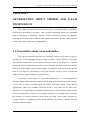
1.1 Research background and motivation ....................................................................1
1.2 Objectives and scope .............................................................................................3
1.3 Thesis structure ......................................................................................................6
2
CHAPTER 2: GENERALITIES ABOUT TIMBER AND X-LAM
TECHNOLOGY ................................................................................................9
2.1 Generalities about wood and timber ......................................................................9
2.2 Load duration and moisture influences on timber strength .................................10
2.3 Timber classification and strength classes ...........................................................13
2.4 Generalities about cross-laminated timber ..........................................................17
2.5 X-Lam panels manufacturing ..............................................................................20
2.6 Advantages of X-Lam technology .......................................................................23
2.7 X-Lam connection systems..................................................................................27
2.7.1
Connections behaviour.............................................................................38
2.7.2
Connections stiffness ...............................................................................38
2.7.3
Connections resistance .............................................................................39
2.8 X-Lam structural applications .............................................................................45
vii
A pre-processor for numerical analysis of cross-laminated timber structures
3
CHAPTER 3: GENERAL ABOUT GID, KRATOS, TCL AND
PYTHON ...........................................................................................................49
3.1 GiD processor ......................................................................................................49
3.1.1
Interaction of GiD with the calculating module ......................................49
3.1.2
GiD Pre-process .......................................................................................52
3.1.3
GiD Post-process .....................................................................................52
3.2 Kratos solver ........................................................................................................53
3.2.1
Kratos advantages ....................................................................................55
3.3 GiD - Kratos interaction ......................................................................................55
3.4 Tcl language.........................................................................................................56
3.5 Python language ...................................................................................................58
4
CHAPTER
4:
MODELLING
STRATEGY
OF
X-LAM
BUILGINGS AND CONVENTIONS ......................................................61
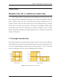
4.1 Modelling strategy ...............................................................................................61
4.2 Modelling of X-Lam panels.................................................................................62
4.3 Connections modelling ........................................................................................65
4.4 Units of measurement convention .......................................................................68
4.5 Gravity convention ..............................................................................................68
5
CHAPTER 5: PRE-PROCESSOR AND INTERFACE TUTORIAL
................................................................................................................................69
5.1 Introduction..........................................................................................................69
5.2 Example introduction...........................................................................................70
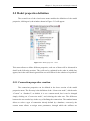
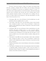
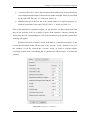
5.3 Problem type selection .........................................................................................71
5.4 Geometry creation ...............................................................................................73
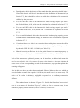
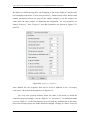
5.5 Model properties definition .................................................................................79
viii
5.5.1
Connection properties creation ................................................................79
5.5.2
Connection properties assignation ...........................................................92
5.5.3
Elements properties creation ....................................................................98
5.5.4
Elements properties assignation .............................................................103
Table of contents
5.5.5
Loads and boundary conditions assignation ..........................................105
5.5.6
Results menu ..........................................................................................106
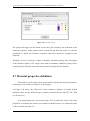
5.6 Group properties definition................................................................................107
5.7 Material properties definition ............................................................................108
5.8 Geometry meshing .............................................................................................111
5.9 File saving ..........................................................................................................113
5.10 Calculation .........................................................................................................114
6
CHAPTER 6: PRE-PROCESSOR PROGRAMMING DETAIL .115
6.1 Surface creation and removal from the menu tree .............................................115
6.2 Line drawing ......................................................................................................116
6.3 New IDs definition ............................................................................................117
6.4 Files writing .......................................................................................................118
6.4.1
Geometry info ........................................................................................119
6.4.2
Connection info ......................................................................................120
6.4.3
Surface element info ..............................................................................122
6.4.4
Line element info ...................................................................................122
6.4.5
More connections ...................................................................................123
6.4.6
More materials .......................................................................................124
6.4.7
Data orthotropic .....................................................................................126
6.4.8
Materials.py ...........................................................................................127
6.5 Connections .......................................................................................................130
6.5.1
Connections stiffness .............................................................................130
6.5.1.1 “Custom-Stiffness” mode ......................................................................130
6.5.1.2 “Custom-Parameters” mode...................................................................131
6.5.1.3 “Standard” mode ....................................................................................133
6.5.2
Connections resistance ...........................................................................135
6.5.2.1 “Custom-Stiffness” mode ......................................................................135
6.5.2.2 “Custom-Parameters” mode...................................................................136
6.5.2.3 “Standard” mode ....................................................................................137
7
CHAPTER 7: MODELLING OF A COMPLEX STRUCTURE ..139
ix
A pre-processor for numerical analysis of cross-laminated timber structures
7.1 Example introduction.........................................................................................139
7.2 Preliminary design phase ...................................................................................141
7.2.1
Static design of X-Lam walls and slabs .................................................142
7.2.2
Seismic design of X-Lam walls and slabs .............................................145
7.2.3
Equivalent static analysis .......................................................................146
7.2.4
Connections seismic design ...................................................................151
7.2.4.1 Shear connections ..................................................................................151
7.2.4.2 Tension connections...............................................................................152
7.2.4.3 Connections stiffness .............................................................................157
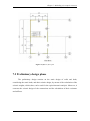
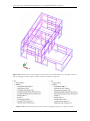
7.3 Modelling ...........................................................................................................157
7.3.1
Geometry ...............................................................................................157
7.3.2
Material and elements properties ...........................................................159
7.3.3
Connection properties ...........................................................................162
7.3.4
Boundary conditions and loads ..............................................................165
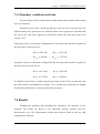
7.4 Results................................................................................................................165
8
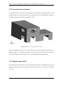
7.4.1
Structure discretization .........................................................................166
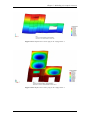
7.4.2
Displacement field .................................................................................166
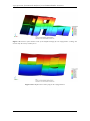
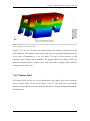
7.4.3
Tension field .........................................................................................169
7.4.4
Reactions ................................................................................................173
CHAPTER 8: CONCLUSION ...................................................................177
8.1 Main contributions .............................................................................................177
8.2 Recommendations for further research ..............................................................178
REFERENCES ........................................................................................................181
x
List of figures
LIST OF FIGURES
Figure 1.1
Example of an offset surface ..................................................................... 5
Figure 1.2
Exploded view of a panel edge.................................................................. 5
Figure 2.1
Effect of moisture content on flexural strength (Giordano 1993)........... 12
Figure 2.2
Effects of timber classification according to resistance (Piazza, Tomasi
and Modena, 2007) ................................................................................. 14
Figure 2.3
Cross-laminated timber panel (ETA-06/0138: 2006) ............................. 18
Figure 2.4
Examples of different cross-sections of X-Lam panels (ETA-06/0138:
2006) ....................................................................................................... 19
Figure 2.5
Manufacturing process of X-Lam panels (FPInnovations, 2013) .......... 22
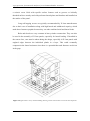
Figure 2.6
Typical three-storey X-Lam building showing various connections
between the X-Lam panels ...................................................................... 28
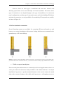
Figure 2.7
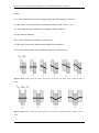
Typical wall-to-foundation X-Lam connections: (a) Connection with an
exposed metal plate; (b) Connection with a concealed connector; (c)
Connection with a wooden profile (FPInnovations, 2013) ..................... 29
Figure 2.8
Typical parallel wall-to-wall X-Lam connections: (a) Connection with an
internal spline; (b) Connection with a surface spline; (c) Connection with
a half-lapped joint; (d) Tube connection system (FPInnovations, 2013)
................................................................................................................. 31
Figure 2.9
Typical perpendicular wall-to-wall X-Lam connections: (a) Connection
with self-tapping screws; (b) Connection with a wooden profile; (c)
Connection with a metal bracket; (d) Connection with a concealed metal
plate (FPInnovations, 2013) ................................................................... 33
Figure 2.10
Typical wall-to-floor X-Lam connections: (a) Connection with selftapping screws; (b) Connection with a metal bracket; (c) Connection
with concealed metal plates (FPInnovations, 2013)............................... 34
Figure 2.11
Typical wall-to-floor X-Lam connections in balloon construction
(FPInnovations, 2013) ............................................................................ 35
Figure 2.12
Typical wall-to-roof X-Lam connections (FPInnovations, 2013) ........... 37
xi
A pre-processor for numerical analysis of cross-laminated timber structures
Figure 2.13
Sihga Idefix innovative connection system (Sihga) ................................. 37
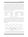
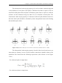
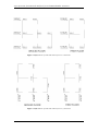
Figure 2.14(a)Failure modes for timber and panel connections with single shear (UNIEN 1995-1-1: 2009) ................................................................................ 42
Figure 2.14(b)Failure modes for timber and panel connections with double shear (UNIEN 1995-1-1: 2009) ................................................................................ 42
Figure 2.14(c) Failure modes for steel-to-timber connections (UNI-EN 1995-1-1: 2009)
................................................................................................................. 43
Figure 2.15
Residential and non-residential X-Lam projects: (a) 10-storey Forté in
Melbourne; (b) 9-storey Stadthaus in London; (c) Open Academy in
Norwich (KLH) ....................................................................................... 47
Figure 3.1
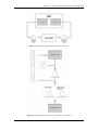
Diagram of GiD workflow (GiD User Manual) ..................................... 51
Figure 3.2
Diagram depicting the files system (GiD User Manual) ........................ 51
Figure 4.1
Orientation of local axes in wall X-Lam panels ..................................... 63
Figure 4.2
Orientation of local axes in a floor X-Lam panel ................................... 63
Figure 4.3
Difference in behaviour between a real and a modelled panel .............. 67
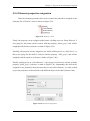
Figure 5.1
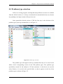
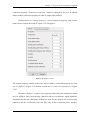
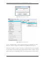
Problem type selection ............................................................................ 71
Figure 5.2
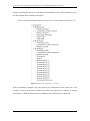
GiD problem types folder........................................................................ 72
Figure 5.3
“Xlam-kratos” command menu .............................................................. 72
Figure 5.4
Gravity warning ...................................................................................... 73
Figure 5.5
“Create object” shortcut ........................................................................ 73
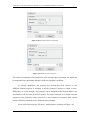
Figure 5.6
First surface ............................................................................................ 74
Figure 5.7
“Copy” menu .......................................................................................... 74
Figure 5.8
“Copy” menu for copying surfaces ........................................................ 75
Figure 5.9
First and second surfaces ....................................................................... 76
Figure 5.10
First, second and third surfaces.............................................................. 76
Figure 5.11
End geometry .......................................................................................... 77
xii
List of figures
Figure 5.12
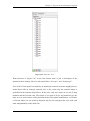
Geometry IDs .......................................................................................... 78
Figure 5.13
“Model properties” menu ....................................................................... 79
Figure 5.14
Custom mode menu ................................................................................. 80
Figure 5.15
“Stiffness” menu ..................................................................................... 81
Figure 5.16
“Connection parameters” menu ............................................................. 83
Figure 5.17
Standard mode menu............................................................................... 86
Figure 5.18
“Connection” menu ................................................................................ 86
Figure 5.19
Hold-down database ............................................................................... 87
Figure 5.20
Brackets and distributed nailings database ............................................ 88
Figure 5.21
"Property1" parameters .......................................................................... 89
Figure 5.22
"Property2" parameters .......................................................................... 90
Figure 5.23
Custom menu with all properties ............................................................ 91
Figure 5.24
Custom menu with all properties and their mode ................................... 91
Figure 5.25
“Surfaces” menu ..................................................................................... 92
Figure 5.26
Geometry created before......................................................................... 93
Figure 5.27
“Delete” shortcut.................................................................................... 93
Figure 5.28
End “Surfaces” menu ............................................................................. 94
Figure 5.29
End geometry .......................................................................................... 95
Figure 5.30
Selection of a connection property ......................................................... 96
Figure 5.31
Drawing of line 2 .................................................................................... 96
Figure 5.32
“Surfaces” menu with assigned connection properties .......................... 97
Figure 5.33
Elements “Properties” menu .................................................................. 98
Figure 5.34
Beam property parameters ..................................................................... 99
Figure 5.35
Solid property parameters ...................................................................... 99
xiii
A pre-processor for numerical analysis of cross-laminated timber structures
Figure 5.36
Shell property parameters..................................................................... 100
Figure 5.37
Elements “Properties” end menu ......................................................... 102
Figure 5.38
“Elements” menu .................................................................................. 103
Figure 5.39
Beam element assignation..................................................................... 103
Figure 5.40
Shell thick element assignation ............................................................. 104
Figure 5.41
Solid element assignation ..................................................................... 104
Figure 5.42
“Elements” end menu ........................................................................... 105
Figure 5.43
“Loads” and “Boundary conditions” menu ......................................... 105
Figure 5.44
“Results” menu ..................................................................................... 107
Figure 5.45
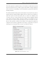
“Groups” menu .................................................................................... 108
Figure 5.46
“Materials” menu ................................................................................. 109
Figure 5.47
Material sub-menu ................................................................................ 110
Figure 5.48
Material creation, removal and renaming window .............................. 111
Figure 5.49
“Mesh generation” window .................................................................. 112
Figure 5.50
Structured mesh selection ..................................................................... 112
Figure 5.51
Meshed geometry .................................................................................. 113
Figure 6.1
“Draw line” section of the code ........................................................... 116
Figure 6.2
“Draw line” groups and geometry ....................................................... 117
Figure 6.3
“More-Materials” file .......................................................................... 125
Figure 6.4
“Materials.py” first section: list of elements properties ...................... 127
Figure 6.5
“Materials.py” added section:”dataOrtho” file reading ..................... 128
Figure 6.6
“Materials.py” added section: matrix creation.................................... 129
Figure 6.7
“Materials.py” added section: composite cross section creation ........ 129
Figure 6.8
Stiffness calculation for “Custom-Parameters” mode ......................... 132
xiv
List of figures
Figure 6.9
Values set in the code for the hold-down WHT340 Φ4*40 with total
nailing ................................................................................................... 134
Figure 6.10
Values set in the code for the bracket WBR100 Φ4*60 with total nailing,
concrete-timber ..................................................................................... 134
Figure 6.11
Values set in the code for the distributed nailing with nail diameter of 4
mm and nail length of 30 mm ................................................................ 134
Figure 6.12
Stiffness calculation for “Standard” mode ........................................... 134
Figure 6.13
Design load-carrying capacities calculation for "Custom-Stiffness” mode
............................................................................................................... 135
Figure 6.14
Design load-carrying capacities calculation for “Custom-Parameters”
mode ...................................................................................................... 136
Figure 6.15
Design load-carrying capacities calculation for “Standard” mode .... 138
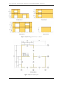
Figure 7.1(a) Building front views A and B ................................................................ 139
Figure 7.1(b) Building front views C, 1, 2 and 3 ........................................................ 140
Figure 7.2(a) Ground floor plan ................................................................................. 140
Figure 7.2(b) First floor plan ...................................................................................... 141
Figure 7.3
Loads analysis....................................................................................... 142
Figure 7.4
Loads representation on the geometry .................................................. 143
Figure 7.5
Preliminary design table for single-span floors (Rothoblaas) ............. 144
Figure 7.6
Preliminary design table for external walls (Rothoblaas).................... 145
Figure 7.7
Afferent heights of the slabs .................................................................. 146
Figure 7.8
Elastic response spectrum for Gerona, Friuli Venezia Giulia, Italy .... 148
Figure 7.9
Barycentre position at the two storeys of the building ......................... 150
Figure 7.10
Selected shear connection (Rothoblaas) ............................................... 151
Figure 7.11
Selected tension connections (Rothoblaas) ........................................... 153
Figure 7.12
Forces causing the first floor rigid rotation ......................................... 154
xv
A pre-processor for numerical analysis of cross-laminated timber structures
Figure 7.13(a)Scheme of walls and relative forces in x-direction ............................... 156
Figure 7.13(b)Scheme of walls and relative forces in y-direction ............................... 156
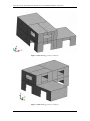
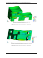
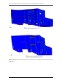
Figure 7.14(a)Building geometry in GiD (a) ............................................................... 158
Figure 7.14(b)Building geometry in GiD (b) ............................................................... 158
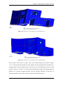
Figure 7.14(c)Building geometry in GiD (c) ............................................................... 159
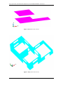
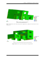
Figure 7.15(a)Floors shell elements ............................................................................ 160
Figure 7.15(b)Walls shell elements .............................................................................. 160
Figure 7.16(a)Curbs beam elements ............................................................................ 161
Figure 7.16(b)Ordinary beam elements ....................................................................... 161
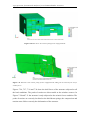
Figure 7.17
Connection property of line 36 belonging to surface 6 ........................ 163
Figure 7.18
Example of line (36) belonging to wall (surface 6) and slab (surface 31);
Example of lines (4 and 5) belonging to walls (surfaces 4 and 5) which
are actually a single wall ...................................................................... 164
Figure 7.19
Connection properties of lines 4 and 5 belonging respectively to surfaces
4 and 5................................................................................................... 164
Figure 7.20
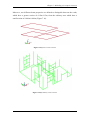
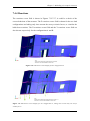
Meshed view of the structure in GiD .................................................... 166
Figure 7.21
X-displacement contour [m] for the configuration A ........................... 167
Figure 7.22
Z-displacement contour [m] for the configuration A............................ 167
Figure 7.23
Contour of the absolute value of the displacement [m] for the
configuration A, taking into account only the storeys seismic forces ... 168
Figure 7.24
Y-displacement contour [m] for the configuration B............................ 168
Figure 7.25
Contour of the absolute value of the displacement [m] for the
configuration B, taking into account only the storeys seismic forces ... 169
Figure 7.26
Shell Force Sxx contour [N/m] for the configuration A ....................... 170
Figure 7.27
Shell Force Syy contour [N/m] for the configuration A ....................... 170
Figure 7.28
Shell Force Szz contour [N/m] for the configuration A, taking into
account only the storeys seismic forces ................................................ 171
xvi
List of figures
Figure 7.29
Shell Force Syy contour [N/m] for the configuration B ....................... 171
Figure 7.30
Shell Force Sxx contour [N/m] for the configuration B ....................... 172
Figure 7.31
Shell Force Szz contour [N/m] for the configuration B, taking into
account only the storeys seismic forces ................................................ 172
Figure 7.32
Z-Reaction vectors display for the configuration A ............................. 173
Figure 7.33
Z-Reaction vectors display for the configuration A, taking into account
only the storeys seismic forces .............................................................. 173
Figure 7.34
Z-Reaction vectors display for the configuration B ............................. 174
Figure 7.35
Z-Reaction vectors display for the configuration B, taking into account
only the storeys seismic forces .............................................................. 174
Figure 7.36
X-Reaction vectors display for the configuration A .............................. 175
Figure 7.37
Y-Reaction vectors display for the configuration B .............................. 175
xvii
List of tables
LIST OF TABLES
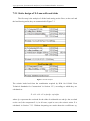
Table 2.1
Load duration classes according to UNI EN 1995-1: 2009 ................... 11
Table 2.2
Values of kmod according to UNI EN 1995-1: 2009 ................................ 13
Table 2.3
Recommended partial factors γM for material properties and resistances
according to UNI EN 1995-1: 2009........................................................ 13
Table 2.4
Strength classes according to EN 338: 2004 for solid wood of conifers
and poplar ............................................................................................... 16
Table 2.5
Strength classes according to EN 338: 2004 for hardwood (poplar
excluded) ................................................................................................. 16
Table 2.6
Values of Kser for fasteners and connectors in N/mm in timber-to-timber
and wood-based panel-to-timber connections, according to UNI-EN
1995-1-1: 2009 (the density ρm is expressed in kg/m3 and the diameter is
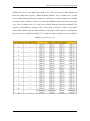
expressed in mm)..................................................................................... 39
Table 6.1
“Geometry-info” file ............................................................................. 119
Table 6.2
“Connection-info” file .......................................................................... 121
Table 6.3
“Surface-element-info” file .................................................................. 122
Table 6.4
“Line-element-info” file........................................................................ 123
Table 6.5
“More-Connections” file ...................................................................... 124
Table 6.6
“Data-Orthotropic” file........................................................................ 126
Table 6.7
“Connection-info” file for line 7 .......................................................... 131
Table 6.8
“Connection-info” file for line 11 ........................................................ 133
Table 6.9
“More-Connections” file for line 7 ...................................................... 136
Table 6.10
“More-Connections” file for line 11 .................................................... 137
Table 7.1
Design concept, structural types and upper limit values of the behaviour
factors for the three ductility classes (EN 1998-1: 2004) ..................... 147
Table 7.2
Storeys seismic forces ........................................................................... 150
xix
A pre-processor for numerical analysis of cross-laminated timber structures
Table 7.3(a) Summary of forces, stresses and hold-down disposed on walls in xdirection ................................................................................................ 155
Table 7.3(b) Summary of forces, stresses and hold-down disposed on walls in ydirection ................................................................................................ 155
xx
Chapter 1: Introduction
CHAPTER 1
INTRODUCTION
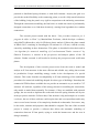
1.1 Research background and motivation
Wood as a building material possesses some inherent characteristics that make
timber structures particularly suited for the use in regions with a high seismic risk, both
due to material properties, such as lightness and load bearing capacity (good weight-tostrength-ratio), and to system properties, like ductility and energy dissipation. Recently,
there have been new developments with prefabricated timber elements, which aim to
address modern building requirements for cost, constructability and structural
performance. Massive cross-laminated timber panels (X-Lam), which can be used as
wall panels, floor panels or roof panels in timber buildings, are becoming a stronger and
economically valid alternative to traditional masonry or concrete buildings in Europe,
and recently also overseas. Especially in seismic-prone countries, X-lam buildings are
gaining more and more popularity. However, due to relatively short time since this
wood engineered product has been launched to the market, the knowledge about crosslam as a structural material is still limited. In recent years, several research projects
around Europe and in North America have been launched, with an aim to better
understand the potential of cross-lam technology as a seismic resistant construction
system.
Still limited is also the knowledge about the modelling of X-Lam structures,
reason why a large research project started to investigate the development of a software
for the analysis, calculation, design and verification of X-Lam structures. This project
was born as collaboration between Padua University and Barcelona’s CIMNE
(International Centre for Numerical Methods in Engineering). Modelling of CLT
buildings lies into properly model the connections between panels; they play an
essential role in maintaining the integrity of the timber structure and providing strength,
stiffness, stability and ductility to the structure. The connections may be modelled with
1
A pre-processor for numerical analysis of cross-laminated timber structures
punctual or distributed spring elements, or with shell elements. Anyway the goal is to
provide the needed flexibility to the connecting points, to avoid a fully unreal behaviour
of the building, being the panels very rigid in comparison to the anchoring connections.
Through the connections modelling, the final aim is to enable the check of preliminarily
designed connections or to find them iteratively, starting from hypothetical or random
connections.
The research project started with the thesis “Una procedura numerica per il
progetto di edifici in Xlam” by Massimiliano Zecchetto, which develops a software,
using MATLAB interface, only for 2D linear elastic analysis. Follows the phase started
in March 2015, consisting in extending the 2D software to a 3D one, with the severity
caused by modelling in three dimensions. This phase is described in this thesis and in
“An algorithm for numerical modelling of Cross-Laminated Timber structures” by
Gabriele D’Aronco; it consists in the pre-process and analysis phases of the 3D
software. Further research is still needed to develop the post-process and verification
phases.
The development of this research project arises from the need to model and
analyse an X-Lam structure in the most efficient and reliable way, taking into account
its peculiarities. Proper modelling strategy results in the development of a special
software. This comes from the non-adaptability to X-Lam technology of the established
procedures for numerical modelling adopted for other types of buildings. Nowadays the
commercial FEM software available do not provide an automatic way to model a CLT
structure. All software, regardless of the strategy chosen for modelling the connections,
only enable to model them manually. For instance, if they are modelled with punctual
springs, the user needs to duplicate the nodes and create the spring elements one by one
at the pre-process interface. Follows that, if the structure is big and complex as it can be
a real one, the use of these software could require time and cost expenditure and it may
cause several errors because of its complexity: hundreds or thousands, if not more, may
be the nodes, elements and properties that should be assigned. The aim of this research
project is exactly to provide a software that allows the automatic modelling of
connections between X-Lam panels, trying to avoid the human error and the cost in
doing it manually.
2
Chapter 1: Introduction
The most convenient strategy for modelling X-Lam structures has to be defined.
Such strategy must be suitable for automatic generation of numerical models and must
have the ability of keeping into account all the possible typologies of connections and
assembling of Cross-Lam panels. In view of future evolution of the research, the
possibility of non-linear behaviour of joints and optimal automatic design via iterative
solutions has to be accomplished too.
1.2 Objectives and scope
The focus of this thesis is on the continuation of the research project on the
development of a software for the modelling of CLT structures, including analysis,
calculation, design and verification of connections and panels. The research work will
include the pre-process phase and the analysis one, the first of which is discussed in this
thesis, the second one in “An algorithm for numerical modelling of Cross-Laminated
Timber structures” by Gabriele D’Aronco.
The procedure is developed using GiD as interface support and processor and
KRATOS Multiphysics as FEM framework. Relatively to the pre-process phase, the
work involved in programming and numerical implementation of the interface and the
data needed for the analysis, by creating a problem type. Relatively to the analysis
phase, the work consisted in the development of the whole procedure of connections
modelling, by creating a new application in Kratos.
Considering the numerical and computational aspects of X-Lam structures,
several are the limits and issues that make it difficult to create models fully
representative of their real behaviour.
Cross-Lam wall panels are very rigid in comparison to the anchoring
connections, so most of the flexibility is concentrated precisely in the latter. To
correctly model the building, avoiding to make it too rigid, the connections are
modelled with punctual spring elements. They enable to simulate the behaviour of the
different kind of connections available in X-Lam technology.
3
A pre-processor for numerical analysis of cross-laminated timber structures
Additionally, a limit lies in the behaviour of the spring elements to use in the
modelling. The behaviour of a CLT structure in static conditions can be assimilated to a
contact problem because the walls are supported all along their lower side by the soil. In
this condition, the walls only work to compression, they do not offer any resistance to
tension. The possible lifting of the walls, which may occur in seismic conditions, is
resisted by the hold-down connections that offer the tension resistance to the walls. To
simulate properly the contact problem, the springs should present a non-linear
constitutive law in axial direction. Alternatively, the problem can be considered nonlinear for the material, considering the hold-down as a material resistant to compression
and the soil as a material non-reactive to traction. Within this project, the springs
present a linear elastic constitutive law, leading to the need of modifying the hold-down
stiffness compared to the real one. This is to take into account the difference in
behaviour, under the action of horizontal forces, of a single modelled panel compared
with the same in a real situation. Therefore, being the spring elements currently added in
Kratos only implemented with linear elastic constitutive law, the analysis is always
considered linear elastic.
In reference to the behaviour of a single X-Lam panel, this is an orthotropic
rather than an isotropic material. This is due to the different total thickness of the layers
in longitudinal and transversal direction and to the difference in value of the elastic
modulus of the timber, which is one order of magnitude greater in the direction parallel
to the grain than in the transversal direction. These two topics lead to adopt an elastic
orthotropic constitutive law for the shell elements.
The research work developed in this common project concerns the creation of a
new problem type, especial for X-Lam structures. It enables the user to model a CLT
structure, starting from the creation of the geometry and the assignation of numeric
entities (beam, shell, ecc) to geometric ones, having defined the material, and assigning
loads and boundary conditions. The user does not need to create manually the
connections, he just set the connection properties to the different sides of the panels.
Also the punctual connections (hold-down) are assigned at the interface to the lines;
conversely, in the analysis they are assigned only to the extreme points of the panel
side.
4
Chapter 1: Introduction
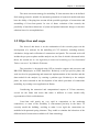
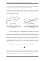
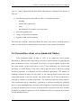
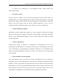
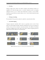
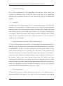
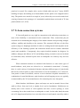
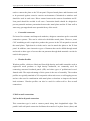
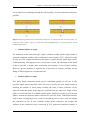
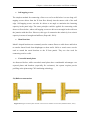
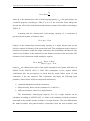
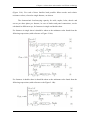
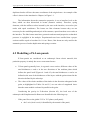
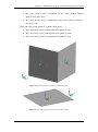
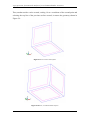
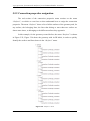
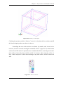
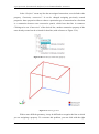
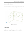
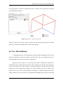
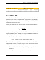
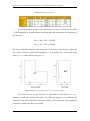
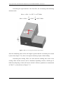
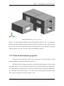
The creation of the connections is made automatically: an abstract offset is
applied between each surface and line, or, better, between each border shell in which the
surface is discretized and beam elements. The information about the connection
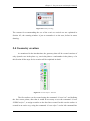
property is stored at interface level to the line (geometric entity), which is discretized,
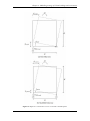
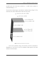
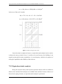
depending on the mesh, in one or more beams (numeric entities). The offset (Figure 1.1)
implies the duplication of the nodes that belong to both beams and shells. It has zero
distance to allow an easy management of the nodes, since the duplicated nodes will
have the same coordinates of the original ones.
Figure 1.1 Example of an offset surface
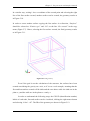
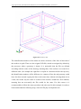
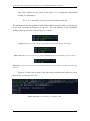
Therefore, spring elements, with the stiffness values inserted by the user at the interface,
are used to join nodes with equal coordinates. The beam elements, necessary for the
duplication of the nodes, are considered fake elements, if not set as curbs at the
interface. Their geometric and structural properties are so that their presence is
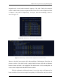
negligible in the analysis of the structure. Figure 1.2 shows the springs connecting the
shells and beams.
Figure 1.2 Exploded view of a panel edge
The pre-process phase, concerning the creation of a new problem type in GiD, is
described in this thesis. It enables, at interface level, the creation of geometry and the
5
A pre-processor for numerical analysis of cross-laminated timber structures
assignation of elements properties, material, loads, boundary conditions and, above all,
connection properties. Moreover, it allows the creation of suitable input data files for
the analysis and the modelling of the panels as orthotropic shells with composite cross
section.
The analysis phase, concerning the numerical changes in Kratos framework, is
described in the thesis “An algorithm for numerical modelling of Cross-Laminated
Timber structures” by Gabriele D’Aronco. It consists in the implementation of spring
elements and the numerical procedure for automatic modelling of the connections,
meaning duplication of panels’ border nodes and joint of nodes by means of spring
elements.
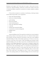
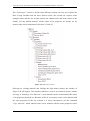
1.3 Thesis structure
A brief summary of each chapter of the thesis is given in this Section. In each
chapter, the first section overviews general information about the chapter topic; in
subsequent sections, theoretical and numerical investigations are described.
Chapter 2 provides an overview of general information about wood, timber and
cross-laminated timber technology. First, influences on timber strength and timber
classification are introduced. Then, description of cross-lam panels and typical X-Lam
connection systems are presented. A state-of-the-art of cross-lam timber application is
highlighted at the end of this Chapter.
Chapter 3 provides an overview of general information about the processor, the
solver and the programming languages used for the thesis: GiD, Kratos, Tcl and Python.
First, description of GiD pre-process and post-process and Kratos tools and advantages
is introduced, up to their interaction; then, a brief description of Tcl and Python features
is presented.
Chapter 4 provides a description of the strategy adopted for modelling CrossLam buildings, explaining in detail panels and connections modelling. At the end of the
Chapter, significant conventions assumed in the modelling are particularised.
6
Chapter 1: Introduction
Chapter 5 provides an extensive explanation of the pre-processor at interface
level. It is a user tutorial, starting from the problem type selection and geometry creation
up to the model properties and material definition, and the calculation of the desired
structure.
Chapter 6 provides an extensive explanation of the pre-processor at
programming level. It presents the code implemented to obtain all the tools of the preprocess, with a detailed description of the files generated by the processor, the
composition of the shell cross section and the calculation of the connections stiffness
and resistance.
Chapter 7 provides a presentation of the modelling of an X-Lam structure case
study, starting from the preliminary design phase up to the actual modelling in GiD,
especially from an engineering point of view. Finally, the results of the analysis are
displayed.
7
Chapter 2: Generalities about timber and X-Lam technology
CHAPTER 2
GENERALITIES ABOUT TIMBER AND X-LAM
TECHNOLOGY
This Chapter presents the main characteristics of wood and timber, providing a
classification according to resistance. Later, general information about cross-laminated
timber technology is displayed. Typical X-Lam connection systems are detailed,
focusing specifically on their stiffness and capacity calculation. Finally, state-of-the-art
of cross-lam timber application is highlighted.
2.1 Generalities about wood and timber
The wood mechanical properties are intimately related to the natural origin of
the material. Cell morphology guarantees high resistance values with low self-weight.
The cellular organization of the wood is however also at the origin of a marked
anisotropy of the mechanical properties of the material, and this results in a marked
difference of the stiffness and resistance values, according to the direction of the applied
load or, in a dual way, depending on the grain direction. Wood is more resistant and
rigid to stresses oriented along the grain direction.
Conversely, solid timber in structural dimensions is a non-homogeneous
material, which contains defects related to the growth of the plant from which it comes,
in the form of nodes, localized grain deviations and many others. These defects
significantly reduce the resistance when the wood is sawn and used for other uses.
Therefore it is evident that the mechanical characteristics of the structural timber cannot
be derived from those of the net wood without taking into account the defects. Besides
the presence of defects within the wood mass, the study of the timber subjected to
external stresses is complicated by the strong influence of moisture variation and load
duration on the resistance.
9
A pre-processor for numerical analysis of cross-laminated timber structures
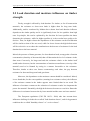
2.2 Load duration and moisture influences on timber
strength
Firstly, strength is affected by load duration. For timber, as for all construction
materials, the resistance to short term loads is higher than for long term loads.
Additionally, studies conducted by Madsen have shown that load duration influence
depends on the timber quality and it is significantly lower for low qualities than high
ones. In principle, this can be explained by the fact that for lower qualities the knots
determine the resistance, while for higher qualities it is the wooden base quality to be
decisive. Thus, for higher classes the dependence of the resistance on the load duration
will be similar to that of the net wood, while for lower classes the high defectiveness
will be so decisive as to reduce the contribution to the decrease of resistance for the load
duration due to the base material.
Indeed, the presence of knots generates, for short duration loads, strong peaks of tension
concentration (elasticity of the material) that will determine the level of resistance in the
short term. Conversely, for long term loads the resistance relative to the timber itself
would tend to decrease, but the concentrations of tensions around knots (viscosity of the
material) tend to be blunted by acting in a manner favourable to the resistance.
Therefore, thanks to these two factors counteracting each other, the gap between
resistance for short and long term loads gets down.
Moreover, the dependence on the moisture content should be considered. Indeed,
it was found that, for the worst qualities (meaning low resistance values), the influence
of the moisture content in the timber appears more limited than in net wood. The
influence of moisture content on the reduction of resistance results less important the
poorer the material. Potentially, the high defectiveness becomes so crucial to flatten the
differences in resistance between the dry base material and the same wet base material.
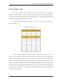
The European regulations (UNI EN 1995-1: 2009) take into account these
influences defining for loads the so-called "load duration classes", and for hygrometric
conditions the so-called "humidity classes" or " service classes".
10
Chapter 2: Generalities about timber and X-Lam technology
The loads are distinguished in permanent loads (always of long duration, of course) and
accidental loads, which may be of long, medium, short term or instantaneous; they are
shown in Table 2.1.
Table 2.1 Load duration classes according to UNI EN 1995-1: 2009
Generally, permanent loads are represented by the weight of the structure, medium term
loads are loads imposed to the slabs (for example, overload for residential use), whereas
snow and wind contribute to short-term, earthquakes to instantaneous loads.
To take into account changes in moisture in the timber, the code prescribes that the
constructions are assigned, depending on the thermo-hygrometric environment, to one
of the following service classes:
Service class 1: this class is characterised by a content of moisture in the
materials corresponding to a temperature of 20 ± 2°C and at a relative humidity
of the surrounding air which exceeds 65% only for a few weeks per year. In the
service class 1 the timber average humidity, in the majority of conifers, is not
greater than 12%.
Service class 2: this class is characterised by a content of moisture in the
materials corresponding to a temperature of 20 ± 2°C and at a relative humidity
of the surrounding air which exceeds 80% only for a few weeks per year. In the
service class 2 the timber average humidity, in the majority of conifers, is not
greater than 20%.
Service class 3: this class includes all climatic conditions which give rise to
higher moisture content in the timber.
11
A pre-processor for numerical analysis of cross-laminated timber structures
To service class 2 belong buildings heated in a non-continuous way and ventilated, such
as houses for leisure, garages without heating, warehouses and cellars.
To service class 3 belong buildings exposed to rainfall or in any case to water, including
the shuttering for the concrete and scaffolding outdoors, as well as support structures of
the roofs not adequately insulated.
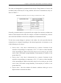
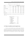
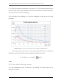
Figure 2.1 Effect of moisture content on flexural strength (Giordano, 1993)
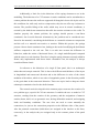
The code UNI EN 1995-1-1: 2009 defines then a correction factor Kmod that
takes into account the effect, on the strength parameters, of both load duration and
moisture content of the structure. In case a combination load includes actions belonging
to different classes of load duration, the code requires the choice of a K mod value that
corresponds to the shorter duration action. The values for the correction factor Kmod
recommended by the code are given in Table 2.2; values are limited to solid timber,
glued laminated timber (to which they refer X-Lam panels) and certain other products
based on timber.
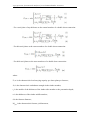
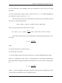
The design value of a generic property of the material can be defined as:
𝑋𝑑 = 𝐾𝑚𝑜𝑑
𝑋𝑘
𝛾𝑀
being γM the partial safety factor for a given material property, Xk the characteristic
value of the same property and Xd its design value. The values for the partial factors γM
recommended by the code UNI EN 1995-1-1: 2009 are given in Table 2.3.
12
Chapter 2: Generalities about timber and X-Lam technology
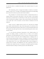
Table 2.2 Values of kmod according to UNI EN 1995-1: 2009
Table 2.3 Recommended partial factors γM for material properties and resistances according to UNI EN
1995-1: 2009
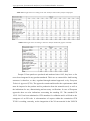
2.3 Timber classification and strength classes
To allow a secure and reliable design of the timber structural elements, the
characteristics of the material must be known with sufficient reliability. The mechanical
characteristics of the wood show a very large dispersion of values; for example the ratio
between the smallest and the largest value of the failure resistance of a sawn wood
element can reach 1:10. This would prevent, in absence of an effective classification,
13
A pre-processor for numerical analysis of cross-laminated timber structures
the use of timber as a structural element properly. The procedure for the classification of
the material is intended to achieve the following goals (with reference to Figure 2.2):
determination of classes of resistance with differentiated properties and reliable
characteristic values;
smaller dispersion of the values of the mechanical properties inside of each class
of resistance compared to the totality of the material (this effect is defined
"homogenisation" of the material).
Figure 2.2 Effects of timber classification according to resistance (Piazza, Tomasi and Modena, 2007)
Numerous and complexes are the factors that can affect the resistance of timber
elements, leading the regulators to adopt an approach consisting in the following points:
selection of elements suitable for structural use and having minimum physicalmechanical guaranteed characteristics (classification according to resistance);
assignment to classified elements of characteristic values of the main mechanical
properties (strength classes and characteristic performance profiles);
design of the elements by means of calculation rules specifically designed to use
these characteristic values.
The method used to define the properties of the timber elements for structural
purposes in the European legislation is the semi-probabilistic limit state. In order to fall
under this methodology it is necessary to abandon the mechanical characterisation of the
14
Chapter 2: Generalities about timber and X-Lam technology
net wood and enlist to a mechanical description of the structural element for a given
applied stress.
The characteristic values of strength and modulus of elasticity are therefore
defined as values to the 5th percentile of the population obtained from tests with loading
time of about 300 seconds on specimens under normal conditions.
The performance of a structural element in timber, as already briefly noted, are
strongly affected by the presence and position, in the same element, of some natural
features that, in structural field, are called defects. For this reason, the structural design
needs a classification according to resistance of the structural element in the dimensions
of use, rather than on the net material, for both elements in laminated wood and
hardwood.
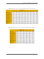
Tables 2.4 and 2.5, adapted from the code EN 338: 2004, show the strength
classes and the related characteristic values of the main properties, for coniferous wood,
poplar wood and hardwood in general. With reference to the glue laminated timber and
X-Lam panels, these tables give the values of some mechanical properties relative to the
slats they contain.
It is clear that the performance characteristics of the finished product, for
example the bending resistance in glulam beams, are related to the resistance
characteristics of the individual boards, as well as, of course, to other aspects related to
the proper execution of butt joints and the bonding between overlapping slats. As
concern the glue-laminated timber elements, excluding the X-Lam panels, the approach
of the new European legislation is to suggest the manufacturer the mechanical features
of the starting sawn to use, to get a glued laminated timber element belonging to a
particular class of resistance. The standard EN 1194: 1999, in particular, provides a set
of relations, here omitted for brevity, for calculation of mechanical properties of timber
laminated elements according to resistance properties of the individual slats.
15
A pre-processor for numerical analysis of cross-laminated timber structures
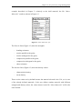
Table 2.4 Strength classes according to EN 338: 2004 for solid wood of conifers and poplar
Table 2.5 Strength classes according to EN 338: 2004 for hardwood (poplar excluded)
Despite X-Lam panels are produced and marketed since 1995, they have so far
never been integrated in any product standards. Their use as a material for load bearing
structures is therefore, to date, regulated through national approvals or by European
Technical Approval (ETA). The approvals contain and describe the requirements which
must be imposed to the product and its production from the materials used, as well as
the indications for use, dimensioning and necessary verifications. In case of European
approvals there are also indications concerning the marking CE. The standard EN
16351: 2013 has been submitted to CEN members for validation and it will lead to the
emergence of an EN code. A subcommittee of experts within the commission CEN
TC250 is working, currently, on the integration of the X-Lam material in the UNI-EN
16
Chapter 2: Generalities about timber and X-Lam technology
1995-1-1: 2009. In particular, the main features that must be evaluated for the release of
ETA are:
load-bearing capacity and stiffness relative to mechanical actions:
-
bending;
-
tension and compression;
-
shear;
-
determination of resistance to bearing stress;
protection against noise;
energy saving and heat retention;
hygiene, health and environment.
Therefore this certificate, which also shows the class of the slats of which the panel is
made, provides all the mechanical features necessary for the structural calculation.
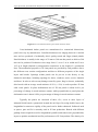
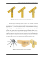
2.4 Generalities about cross-laminated timber
Cross laminated timber (X-Lam or CLT) is an engineered wood product
fabricated by adhering and compressing wood layers called lamellae in perpendicular
grain orientations to form a solid panel. Wood layers are glued together on their wide
faces and, usually, on the narrow faces as well. X-Lam technology was invented and
developed in central Europe in the early 1990‘s and since then it has been gaining
increased popularity in residential and non-residential applications. The number of
buildings constructed using X-Lam panels as the main structural system has seen
exponential growth in the last decade, and market share for X-Lam construction is
expected to continue to escalate in the future. The European experience showed that XLam construction can be competitive, particularly in mid-rise and high-rise buildings
due to its easy handling during construction and a high level of prefabrication. Recently,
X-Lam was introduced also overseas, in North America, Australia and in New Zealand.
A number of production plants have been established or they are proposed to be built in
aforementioned countries.
17
A pre-processor for numerical analysis of cross-laminated timber structures
Figure 2.3 Cross-laminated timber panel (ETA-06/0138: 2006)
Cross-laminated timber panels are manufactured to customized dimensions;
panel sizes vary by manufacturer. Lamellae thicknesses are ranging between 10 and 40
mm, and are produced of technically dried, quality-sorted and finger-jointed planks.
Panel thickness is usually in the range of 50 mm to 300 mm but panels as thick as 500
mm can be produced. Production sizes range from 1.2 m to 3 m in width and 5 m to
16.5 m in length (limited by transportation restrictions or the length of a production
line). The mechanical properties of X-Lam panels are provided by each producer due to
the different cross section configurations and due to different properties of the single
layers and boards. Openings within panels can be pre-cut in the factory to any
dimension and shape, including openings for doors, windows, stairs, service channels
and ducts. In order to rule out any damage caused by pests, fungi or insects, technically
dried wood with an average wood moisture of 12% (+/-2%) is used to produce X-Lam
solid wood panels. In plane deformation rate of X-Lam panels is about 0.01% per
percentage of change in wood moisture content, while perpendicular to panel plane the
deformation rate is about 0.20% per percentage of change in wood moisture content.
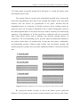
Typically the panels are consisted of three, five, seven or more layers of
industrial dried boards, symmetrical around the mid layer. By using double layers, the
longitudinal or transverse rigidity of the panel can be further enhanced. Softwood such
as spruce, pine and fir is currently used in X-Lam production. Boards with different
grading classes might be used for longitudinal (parallel) and transversal (perpendicular)
layers to optimise mechanical and fire performances of X-Lam product. The density of a
18
Chapter 2: Generalities about timber and X-Lam technology
CLT timber panel is generally around 400 to 500 kg/m3 i.e. around the density of the
base laminate species used.
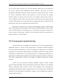
The external loads are carried by the longitudinal (parallel) layers, whereas the
transversal (perpendicular) layers have lower strength and stiffness in the main panel
direction since the stresses are perpendicular to the grains. Provided that the
longitudinal layers are connected via flexible transverse layers, bending caused by
transverse forces can no longer be disregarded. The so-called “rolling-shear” (shear in
the radial-tangential-plane) in the transversal layers leads to relatively low load-bearing
capacities. Cross-lamination in X-Lam panels have reinforcing effect for prevention
from brittle failure modes such as splitting, and increases strength capacity of
connections. The cross-laminating process provides improved dimensional stability to
the product which allows for prefabrication of long and wide panels. Additionally,
cross-laminating provides relatively high in-plane and out-of-plane strength and
stiffness properties, giving it two-way action capabilities similar to a reinforced concrete
slab.
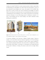
Figure 2.4 Examples of different cross sections of X-Lam panels (ETA-06/0138: 2006)
By varying the number of layers as well as the lumber species, grade and
thickness, X-Lam panels can be used in various assembly types such as walls, floors,
19
A pre-processor for numerical analysis of cross-laminated timber structures
roofs, elevator shafts, stairways etc. The wall and floor panels may be left exposed in
the interior, which provides additional aesthetic attributes. The panels are used as
prefabricated building components which can speed up construction practices or allow
for off-site construction. While X-Lam panels act as two-way slabs, the stronger
direction follows the grain of the outer layers. For example, when used for walls, XLam is installed so the boards on the outer layer of the panel have their grain running
vertically. When panels are used in floor and roof applications, they are installed so the
boards on the outer layer run parallel to the span direction.
Panels may be connected to each other with half-lapped, single or double splines
made from engineered wood products. Dowel-type mechanical fasteners such as nails,
screws, dowels and bolts, or bearing-type (e.g., split rings, shear plates) connectors are
used to connect X-Lam panels. Typical X-Lam connections will be presented more in
detail in Section 2.7 of this Chapter.
2.5 X-Lam panels manufacturing
Currently there are no standards in Europe that cover X-Lam manufacturing or
installation. However, various X-Lam products have a European Technical Approval
(ETA) that allows manufacturers to place CE marking. The approval process includes
preparation of a European Technical Approval Guideline (ETAG) that contains specific
requirements of the product as well as test procedures for evaluating the product prior to
submission to the European Organization for Technical Approvals (EOTA). Finally, the
ETA allows manufacturers to place CE marking (Conformité Européenne) on their
products.
In the USA, the American National Standards Institute (ANSI) recently
approved ANSI/APA PRG 320-2012 Standard for Performance-Rated Cross-Laminated
Timber (ANSI/APA PRG 320-2012, 2012). This Standard covers manufacturing,
qualification and quality assurance requirements for X-Lam products. Key stakeholders
included X-Lam manufacturers, distributors, designers, users, building code regulators,
and government agencies.
20
Chapter 2: Generalities about timber and X-Lam technology
In general, the production of cross-laminated timber panels follows the
following procedure:
Selection of species
The base species of timber used for X-Lam panels depend on the region where it is
manufactured. For X-Lam manufactured in Austria and Germany spruce is the main
species used; pine and larch can also be used on request. X-Lam plants in Canada are
likely to use S-P-F (spruce pine fir) species. Whilst production is yet to occur in
Australia and New Zealand, the timber species likely to be used is radiata pine.
Timber laminates grouping
Individual seasoned dimensional timbers are used, generally softwood and usually
finger jointed along their length to obtain the desired lengths and quality. Individual
timbers can be edged bonded together to form a timber plate before further assembly
into the final panel.
Adhesive application
Generally the choice of adhesives is dependent on manufacturers but the new
polyurethane (PUR) adhesives are normally used as they are formaldehyde and solvent
free. Occasionally, and manufacturer dependent, melamine urea formaldehyde and
phenol-resorcinol-formaldehyde adhesives could be used. Both face and edge gluing
can be applied.
Panel assembly and arrangement
The main difference that occurs between X-Lam manufacturers is the treatment of
individual layers. Some manufacturers edge bond the individual dimensional timber
together to form a layer before pressing each layer into the final X-Lam panel. Other
manufacturers just face bond individual dimensional timber in layers and press all of
them together into the final X-Lam panel in the one operation. Panel sizes vary by
manufacturer and application, as mentioned in the beginning in this Chapter.
21
A pre-processor for numerical analysis of cross-laminated timber structures
Pressing
Gluing at high pressure reduces the timbers expansion and shrinkage potential to a
negligible level, thus the right pressure is essential. Hydraulic presses are normally
employed, however, use of vacuum and compressed air presses is also possible,
depending on panel thickness and the adhesive used. Vertical and horizontal pressings
can be applied.
Planing and sanding
The assembled X-Lam panels are planed or sanded for a smooth surface finish.
Panel final shaping
Computer numerical controlled (CNC) routers are generally used to cut the X-Lam
panel to the final length and width. Sometimes manufacturers also pre-cut openings for
windows, doors and service channels, connections and ducts. The addition of insulation
and exterior cladding may also take place in the factory, and the completed panels are
shipped to the job site ready to be erected into place.
Figure 2.5 Manufacturing process of X-Lam panels (FPInnovations, 2013)
22
Chapter 2: Generalities about timber and X-Lam technology
2.6 Advantages of X-Lam technology
X-Lam technology has several advantages in structural applications:
Low weight
The X-Lam buildings can weigh up to four times less than its concrete counterpart,
which can reduce transportation costs, allows the designers to reduce the foundation
size, and eliminate the need for a tower crane during construction (Yates et al., 2008).
Mobile cranes can be employed, saving substantial erection, hire and labour costs.
Prefabrication
The prefabricated nature of X-Lam technology permits high precision in terms of
dimensional accuracy due to CNC controlled cutting and quality controlled production.
Wall, floor and roof elements can be pre-cut, including openings for doors, windows,
stairs, service channels and ducts. Insulation and finishes can also be applied prior to
installation, reducing demand for skilled workers on site. Construction process is
characterized by increased safety on the construction site, faster project completion and
availability for occupancy in a shorter time. For example, it took four carpenters just
nine weeks to erect nine storeys and the entire construction process was reduced from
72 weeks to 49 weeks (Yates et al., 2008) compared to a traditional reinforced concrete
building. In addition, there is less disruption to the surrounding community and less
waste is produced. As most of the work occurs off-site at the factory, there is a lower
demand for skilled workers on-site.
Easy handling and erection
Handling the X-Lam panels requires smaller cranes which also influences on the lower
cost of a building construction. One of the biggest benefits of using X-Lam panels is
that the structure can be built quickly and efficiently. Because panels are designed for
specific end-use applications, they are often delivered and erected using a “just-in-time”
construction method, making X-Lam ideal for projects with limited on-site storage
capacity. Panels are usually loaded into the truck at the manufacturing plant in the
sequence that they will be required for installation on site. Where it is not possible to
23
A pre-processor for numerical analysis of cross-laminated timber structures
install X-Lam panels immediately, they can be off-loaded and stored off the ground
under a waterproof covering until required. Due to the light weight of the panels it is
also common to use the building itself as a place to temporarily store panels. It is also
possible to assemble elements or modules of the building off-site and deliver completed
segments of the building to the site. This speeds up the construction process even
further. Panels are lifted into place using pre-inserted hooks.
Flexibility in architectural implementation
Versatility of X-Lam technology comes from the fact that panels can be used for many
different assemblies (wall, floor, roof, stairs etc.) just by varying the thickness. X-Lam
construction system can be combined also with other timber structural systems such as
light timber frames, post-and-beam heavy timber system and glue-laminated timber. In
addition, X-Lam elements are compatible with other building materials such as steel,
concrete and glass. Compared to traditional light wood-frame construction methods,
which rely on plywood sheathing over wood studs (walls) or rafters and beams (roof),
the use of X-Lam panels offers an alternative in the form of a single component that is
load bearing and provides an aesthetically pleasing finished surface. Depending on its
intended use, X-Lam panels can be used for either visible or hidden construction
applications. Its ability to be used as either a panelised or a modular system makes it
ideally suited for additions to existing buildings or their upgrade. Good span-to-depth
ratio allows shallow floors and slender construction elements can increase the net
building are.
Static properties
High in-plane and out-of-plane strength and stiffness properties of X-Lam panels enable
in-plane stability of the panels and lack of susceptibility to soft-storey failures. The
cross-lamination provides relatively high strength and stiffness properties in both
directions, giving it a two-way action capability similar to a reinforced concrete slab.
Seismic performance
In terms of seismic performance, timber buildings in general perform well because
wood is relatively light as a construction material, thus inertial forces caused by
24
Chapter 2: Generalities about timber and X-Lam technology
earthquakes are lower than in case of buildings made of other materials. High ductility
and energy dissipation capacities of X-Lam buildings, together with sufficient strength
capacity, make this construction system very effective at resisting lateral forces caused
by earthquake ground motions.
Fire resistance
X-Lam assemblies have inherently excellent fire-resistance due to the thickness of
panels, which when exposed to fire, slow down the heat propagation within the cross
section and char at a slow and predictable rate (0.67 mm/min according to ETA 06/0138, 2006). Once formed, this char protects the wood from further degradation,
helping to maintain structural integrity of the building. In addition, X-Lam structures
also tend not to have as many concealed spaces within floor and wall assemblies, which
reduces the risk of a fire spreading. Fire performance of X-Lam panels can also be
enhanced by lining with fire resisting gypsum boards and, in case of floor panels,
additional layers and coverings. A demonstration test conducted by IVALSA on a full
scale, three-storey X-Lam building confirmed that X-Lam panels protected by one layer
of gypsum board were able to withstand the burn out of the room contents without fire
spread to adjacent rooms or floors (Frangi et al., 2008).
Thermal performance
Cross-lam panels have the same fundamental thermal insulation and thermal mass
properties as the wood from which they are made (thermal conductivity λ = 0.13
W/(m*K) according to EN 12524, 2000). Wood has a low thermal conductivity so
reduces problems such as thermal bridging from the internal to the external
environments and the other way around, thus reducing heat transfer and energy wastage.
Acoustic performance
Solid wood panels offer acoustical advantages when used for floor and wall systems.
When used in conjunction with insulation and gypsum board, it is possible for an XLam building to exceed code requirements related to the acoustical performance of
floors and walls.
25
A pre-processor for numerical analysis of cross-laminated timber structures
Dimensional stability
The crosswise arrangement of the longitudinal and transverse layers reduces the
swelling and shrinkage of the wood in the plane of the panel to an insignificant
minimum and considerably increases the static load-carrying capacity and dimensional
stability.
Durability
Generally due to the quick erection time of X-Lam based systems, the short term
exposure of X-Lam panels to weather is not an issue. Short term and occasional
exposure to water will not have long term effect on X-Lam panels. During construction
wall elements may be protected with vapour barriers or the building’s scaffolding can
be wrapped to form this protection. Other strategies could be employed such as coating
system for the construction period only. Long-term exposure of X-Lam panels to
weather is not recommended.
Sustainable and environmental friendly building material
As with all wood products, the benefits of X-Lam include the fact that wood grows
naturally, using solar energy and it is the only major building material that is renewable
and sustainable. It also has a low carbon footprint, because the panels continue to store
carbon absorbed during the tree‘s growing cycle and because of the greenhouse gas
emissions avoided by not using products that require large amounts of fossil fuels to
manufacture. Harvesting from sustainably managed forests contribute to efficient use of
the resource. Many of the recent structures built from CLT benefit from these
environmental considerations. For example, two mid-rise residential projects in London
used the fact that wood stores carbon and that substantial greenhouse gas emission were
avoided by substituting cross-lam in place of concrete or steel to get preferential
approval from local planning authorities (Yates et al., 2008).
Recycling and reuse
X-Lam panels can also be recycled and reused for the same or for a different purpose.
Structural flexibility of the panels is very wide as well as their durability, thus enabling
26
Chapter 2: Generalities about timber and X-Lam technology
panels to be reused. For example, after a series of shake table tests on a 7-storey SOFIE
building in Japan, the building was disassembled and the panels were shipped back to
Italy. The panels were stored for a couple of years, before they were used as main loadcarrying elements in the prototype of a sustainable modular house unit made of X-Lam
panels (Briani et al., 2012).
2.7 X-Lam connection systems
X-Lam wall panels are very rigid in comparison to the anchoring connections, so
most of the flexibility is concentrated in the connections. Thus, connections play an
essential role in maintaining the integrity of the timber structure and providing strength,
stiffness, stability and ductility to the structure. The structural efficiency of the floor
system acting as a diaphragm and that of walls in resisting lateral loads depends on the
efficiency of the fastening systems and connection details used to connect individual
panels and assemblies. Consequently, they require detailed attention by designers. In
addition, damages and failures in X-Lam buildings during a seismic event are localized
in connections; thus, structural repairs after an earthquake are relatively easy and cost
effective.
When structural members are attached with fasteners or some other types of
metal hardware, such joints are referred to as “mechanical connections”. Currently,
there is a wide variety of mechanical fasteners and many different types of joint details
that can be used for panel to panel connections in X-Lam assemblies or to connect XLam panels to other wood-based, concrete or steel elements in hybrid construction. A
combination of metal hold-downs, angle brackets and self-tapping screws are typically
recommended by the X-Lam manufacturers for connecting the cross-lam panels.
Metal brackets, hold-downs, plates and straps are used to transfer forces from
walls to floors, from one level to another level, and to foundations. Hold-downs are
mainly used in the corners of wall segments and close to door opening, to resist
overturning forces that result from an earthquake or wind. On the other hand, the main
role of L-shaped metal brackets is to resist shear forces in wall panels caused by wind or
27
A pre-processor for numerical analysis of cross-laminated timber structures
a seismic event. Nails with specific surface features such as grooves or helically
threaded nails are mostly used with perforated metal plates and brackets and installed on
the surface of the panel.
Long self-tapping screws are typically recommended by X-Lam manufacturers
due to their ease of installation along with high lateral and withdrawal capacity, which
make these fasteners popular because they can take combined axial and lateral loads.
Bolts and dowels are very common in heavy timber construction. They can also
be used in the assembly of X-Lam panels, especially for lateral loading. If installed in
the narrow face, care must be taken during the design, especially in X-Lam panels with
unglued edges between the individual planks in a layer. This could eventually
compromise the lateral resistance since there is a potential that such fasteners are driven
in the gaps.
Figure 2.6 Typical three-storey X-Lam building showing various connections between the X-Lam panels
28
Chapter 2: Generalities about timber and X-Lam technology
However, there are other types of traditional and innovative fasteners and
fastening systems that can be used efficiently in X-Lam assemblies. The choice of the
type of connection to use depends largely on the type of assemblies to be connected,
panel configurations, and the type of structural system used in the building. With these
mechanical connections, several possibilities for assembling X-Lam panels are possible,
as shown in Figure 2.6.
1. Wall-to-foundation connections
Several fastening systems are available for connecting X-Lam wall panels to steel
beams or to concrete foundations with concrete footing, which are most common for the
ground storeys in X-Lam buildings.
Figure 2.7 Typical wall-to-foundation X-Lam connections: (a) Connection with an exposed metal plate;
(b) Connection with a concealed connector; (c) Connection with a wooden profile (FPInnovations, 2013)
Visible or exposed metal plates
Exterior metal plates and brackets are commonly used in such applications as there is a
variety of such metal connectors readily available on the market and due to its simple
installation. Lag screws or powder-actuated fasteners can be used to connect the metal
plate to the concrete footing or slab, while nails, lag screws or self-tapping screws are
29
A pre-processor for numerical analysis of cross-laminated timber structures
used to connect the plate to the X-Lam panel. Exposed metal plates and fasteners need
to be protected against corrosive exterior environments. Galvanized or stainless steel
should be used in such cases. Direct contact between the concrete foundation and XLam panel should be avoided in all cases. Connection details should be designed to
prevent potential moisture penetration between the metal plates and the X-Lam wall as
water may get trapped and cause potential decay of the wood.
Concealed connectors
For better fire resistance and improved aesthetics, designers sometimes prefer concealed
connection systems. This can be achieved with hidden metal plates. However, some
CNC machining work is required to produce the grooves in the X-Lam panel to conceal
the metal plates. Tight dowels or bolts can be used to attach the plates to the X-Lam
panel. In addition, some innovative types of fasteners that can be drilled through metal
and wood or other types of screws that can penetrate through both materials can also be
used for this purpose.
Wooden Profiles
Wooden profiles, which are fabricated from high density and stable materials such as
engineered wood products or high density hardwood, are commonly used for
connecting structural insulated panels (SIP) and other types of prefabricated woodframed walls. The major advantage of this system is the ease of assembly. The wooden
profiles are typically attached to X-Lam panels with wood screws or self-tapping screws
and are often used in combination with metal plates or brackets to improve the lateral
load resistance. Wooden profiles can also be used for wall-to-wall or floor-to-wall
connections.
2. Wall-to-wall connections
2a) Parallel wall panel connection
This connection type is used to connect panels along their longitudinal edges. The
parallel wall-wall panel connection facilitates the transfer of in-plane forces (shear) and
30
Chapter 2: Generalities about timber and X-Lam technology
out-of-plane forces (bending) through the wall assembly. Several connections details are
possible.
Figure 2.8 Typical parallel wall-to-wall X-Lam connections: (a) Connection with an internal spline; (b)
Connection with a surface spline; (c) Connection with a half-lapped joint; (d) Tube connection system
(FPInnovations, 2013)
Internal splines or strips
For formation of this connection type, single or double wooden splines (strips) made of
structural composite lumber, such as laminated veneer lumber (LVL), plywood or thin
X-Lam, are used. Connection between the spline or splines and the panel edges can be
established using self-tapping screws, wood screws or nails. The advantage of this detail
is that it provides a double shear connection and resistance to out-of-plane loading.
However, special attention is required due to necessity of accurate profiling for the
fitting of different parts on a construction site.
Surface splines or strips
This fairly simple connection detail can be established quickly on site but it only
provides single shear connection. Since two sets of screws are used, which results in
doubling the number of shear planes resisting the load, a better resistance can be
achieved using this detail. Panel edges are profiled from one side for a single surface
spline or from both sides for a double surface spline. Similarly as in the case of internal
splines, structural composite lumber elements are used for strips. Traditional fasteners
such as nails, self-tapping screws, wood screws and lag screws can be used for making
the connection on site. In case of double surface spline connection, the strength and
stiffness of the connection can be increased. If SCL (structural composite lumber) is
31
A pre-processor for numerical analysis of cross-laminated timber structures
used as the spline, the joint can be designed to resist moment for out-of-plane loading
(Augustin, 2008). Structural adhesives could be used to enhance the strength and
stiffness.
Half-lapped joint
In this connection type, long self-tapping screws are usually used to connect the panel
edges. The joint can carry normal and transverse loads but it is not considered to be a
moment resisting connection (Augustin, 2008). This connection detail is considered as
very simple, so it facilitates quick assembly of X-Lam elements. However, there is a
risk of splitting of the cross section due to concentration of tension perpendicular to
grain stresses in the notched area. This is particularly emphasized for cases where
uneven loading on the floor elements occur (Augustin, 2008).
Tube connection system
Tube connection system incorporates a profiled steel tube with holes in the X-Lam
panel. Panel elements are delivered on site with glued-in or screwed rods driven in the
plane of the two panels which are supposed to be connected. The tube connector is
inserted at certain locations along the edges of the panels where the metal tubes are to
be placed. The system is tightened on site using metal nuts. Usually no edge profiling
along the panel is needed as it relies principally on the pull-out resistance of the screwed
or glued-in rods (Traetta, 2007).
2b) Perpendicular wall panel connection
This Section presents connection details for connecting wall panels to wall panels
positioned at right angles (transverse direction). Such connection details include interior
partition walls to exterior walls or just exterior corner walls. Several systems have been
adopted to establish connection between perpendicular walls.
32
Chapter 2: Generalities about timber and X-Lam technology
Figure 2.9 Typical perpendicular wall-to-wall X-Lam connections: (a) Connection with self-tapping
screws; (b) Connection with a wooden profile; (c) Connection with a metal bracket; (d) Connection with
a concealed metal plate (FPInnovations, 2013)
Self-tapping screws
This is the simplest form of connecting X-Lam wall panels together. There are some
concerns related to this form of connection due to the fact that the screws are driven in
the narrow side of panels, in particular if screws are installed in the end grain of the
cross layers. Self-tapping screws can be driven straight into the X-Lam panel or at an
angle to avoid direct installation of screws in the narrow side of the panel.
Wooden profiles
Concealed wooden profiles or keys can also be used in a similar way, with self-tapping
screws or traditional wood screws. The advantage of this system over the direct use of
self-tapping screws is the possibility of enhancing the connection resistance by driving
more wood screws to connect the profiled panel to the central wood profile which is in
turn screwed to the transverse wall.
Metal brackets
Another simple form of connecting walls in the transverse direction is the use of metal
brackets with screws or nails. This connection system is one of the simplest and most
efficient types of connection in terms of strength resulting from fastening in the
33
A pre-processor for numerical analysis of cross-laminated timber structures
direction perpendicular to the plane of the panels or recessed. However, adding
protective membrane (i.e., gypsum board) for improved fire resistance is required.
Concealed metal plates
As previously discussed, while it has considerable advantages over exposed plates and
brackets, especially when it comes to fire resistance, this system requires precise
profiling at the plant using CNC machining technology. Self-drilling dowels that can
penetrate through wood and steel can also be used. Metal plate thickness ranges from 6
mm up to 12 mm.
3. Wall-to-floor connections
Several possibilities exist when it comes to connecting walls to the floors above,
depending on the form of structural systems (i.e., platform or balloon), on the
availability of fasteners and the degree of prefabrication.
3a) Platform construction
Figure 2.10 Typical wall-to-floor X-Lam connections: (a) Connection with self-tapping screws; (b)
Connection with a metal bracket; (c) Connection with concealed metal plates (FPInnovations, 2013)
34
Chapter 2: Generalities about timber and X-Lam technology
Self-tapping screws
The simplest method for connecting a floor or a roof to walls below is to use long selftapping screws driven from the X-Lam floor directly into the narrow side of the wall
edge. Self-tapping screws can also be driven at an angle to maximize the fastening
capacity in the panel edge. The same principle could be applied for connecting walls
above to floors below, where self-tapping screws are driven at an angle in the wall near
the junction with the floor. However, this type of connection has relatively low seismic
capacity in terms of strength and stiffness (Popovski, 2010).
Metal brackets
Metal L-shaped brackets are commonly used to connect floors to walls above and below
to transfer lateral loads from diaphragm to shear walls. Nails or wood screws can be
used to attach the metal brackets to the X-Lam panels. They are also used for
connecting roofs to walls.
Concealed metal plates
As discussed before, while concealed metal plates have considerable advantages over
exposed plates and brackets (especially fire resistance), the system requires precise
profiling at the plant using CNC machining technology.
3b) Balloon construction
Figure 2.11 Typical wall-to-floor X-Lam connections in balloon construction (FPInnovations, 2013)
35
A pre-processor for numerical analysis of cross-laminated timber structures
In Europe, the most common type of structural form in X-Lam construction is the
platform type of system due to its simplicity in design and erection. However, in nonresidential construction, including industrial buildings, it is common to use tall walls
with an intermediate floor between the main floors of a building. So called “mezzanine
floor” is often located between the ground floor and the first floor. However, it is not
unusual to have a mezzanine in the upper floors of a building. Several attachment
options to connect X-Lam floor to a continuous X-Lam tall wall exist for such
applications. The simplest attachment detail includes the use of a wooden ledger (made
of structural composite lumber) to provide a continuous bearing support to the X-Lam
floor panels. Another type of attachment is established with the use of metal brackets.
Attachment of wooden ledger or metal brackets to the X-Lam wall and floor panels is
established through the use of screws, lag screws or nails. However, out-of-plane
bending due to wind suction could be an issue with this type of detail and designers
need to take that into account.
4. Floor-to-floor connections
When the connection is used in floor assemblies acting as diaphragms, the connection
must be capable of transferring in-plane diaphragm forces in principle, and maintain the
integrity of the diaphragms. Connection details used in floor-to-floor panel connection
are equal to parallel wall-to-wall panel connection types, described earlier in this
Chapter.
5. Wall-to-roof connections
For sloped or flat roof systems, connections similar to those used for attaching floors to
walls is used. Screws and metal brackets are the most commonly used fastening systems
in this application.
36
Chapter 2: Generalities about timber and X-Lam technology
Figure 2.12 Typical wall-to-roof X-Lam connections (FPInnovations, 2013)
Innovative types of connection systems can also be used, including mechanical
and carpentry connection systems. Some interesting innovative connection systems are
finding their way to the X-Lam construction market, mostly facilitated and enabled by
CNC technology. For example, glued-in rods can be used for connections under high
longitudinal and transverse loads. HBV-Shear Connectors, a proprietary product from
Germany, can also be used to create composite floors with structural concrete over XLam panels (Bathon & Bletz, 2006). Further, KNAPP system (Knapp) and Idefix
connectors (Sigha) are relatively new innovative connection systems on the market. Due
to the relatively recent introduction of X-Lam technology into the construction market,
it is expected that even more new connection types will be developed over time.
Figure 2.13 Sihga Idefix innovative connection system (Sihga)
37
A pre-processor for numerical analysis of cross-laminated timber structures
2.7.1 Connections behaviour
About the kinematic behaviour of the connections, it can be assumed that:
1. the shear connections (angle brackets, shear screws,...) do not work in tension;
2. the tension connections (hold-down) do not work in shear.
These two hypotheses are, nowadays, widely used in the calculation of X-Lam
buildings and they are assumed to be valid in this thesis. However, if on one hand they
allow to greatly simplify the calculations, on the other hand they do not take into
account the actual failure behaviour of the panels. The behaviour of an X-Lam panel
subjected to horizontal forces is a combination of horizontal sliding and rigid rotation
(rocking); consequently, all connections at the base are subjected to a combination of
horizontal forces, or shear forces, and lifting. For further information about the
behaviour of an X-Lam panel subjected to horizontal forces, see the thesis “Una
procedura numerica per il progetto di edifici in X–Lam” by Massimiliano Zecchetto.
Relatively to the first assumption, different theoretical models have been
proposed in order to take into account the actual presence of angle brackets in the
rocking effect (Gavric and Popovski, 2014). In this case, the interaction between shear
and tension, to which the angle brackets are subjected, must also be considered. Finally,
it results necessary to define a domain of resistance in the plane N - V.
Regarding the second assumption, the hypothesis is fully confirmed by
experimental research on X-Lam walls (Popovski, 2010) and on individual connecting
elements (Gavric, Fragiacomo and Ceccotti, 2014).
2.7.2 Connections stiffness
Regardless of the behaviour of the connections, shear or tension, the code UNIEN 1995-1-1:2009 provides the relations for the calculation of the slip modulus kser per
shear plane per fastener, which are shown in Table 2.6.
38
Chapter 2: Generalities about timber and X-Lam technology
Table 2.6 Values of Kser for fasteners and connectors in N/mm in timber-to-timber and wood-based
panel-to-timber connections, according to UNI-EN 1995-1-1: 2009 (the density ρm is expressed in kg/m3
and the diameter is expressed in mm)
The slip modulus kser for fasteners in timber-to-steel connections is equal to two times
the slip modulus in timber-to-timber connections.
Once identified the stiffness per shear plane per fastener, the stiffness of the
brackets or distributed nailing and hold-down can be calculated.
The stiffness of the brackets is obtained by simply multiplying kser by the total number
of nails of the connection (meaning the number of nails if only one bracket or a
distributed nailing is disposed, the number of nails multiplied by the number of brackets
if more than one bracket are disposed).
Similarly, the stiffness of the hold-down can be calculated by multiplying kser by the
total number of nails of the connection (meaning the product between the number of
nails of each hold-down and the number of hold-down). However, in this case, the
stiffness inserted in the model does not coincide with the stiffness value suggested by
the code. This comes from the difference in behaviour, under the action of horizontal
forces, of a single modelled panel compared with the same in a real situation (see
Section 4.3).
2.7.3 Connections resistance
The design resistance of a connection Rd (load-carrying capacity) can be
calculated as:
39
A pre-processor for numerical analysis of cross-laminated timber structures
𝑅𝑑 = 𝑘𝑚𝑜𝑑
𝑅𝑘
𝛾𝑀
where Rk is the characteristic value of load-carrying capacity, γM is the partial factor for
a material property (according to Table 2.3), kmod is the correction factor taking into
account the effect of the load duration and moisture content of the timber (according to
Table 2.2).
Assuming that the characteristic load-carrying capacity of a connection is
governed by the number of fasteners, then:
𝑅𝑘 = 𝜂𝑒𝑓𝑓 ∙ 𝐹𝑉,𝑅𝑘
being FV,Rk the characteristic load-carrying capacity of a single fastener and ηeff the
effective number of fasteners of the connection itself. This assumption leads to impose a
hierarchy of resistance within the single connection; the relationship considered is only
valid in case of failure of the connection on the fasteners and not on the steel plate. The
resistance of the connection would actually be equal to:
𝑅𝑘 = 𝑚𝑖𝑛 {
𝑅𝑝𝑙𝑎𝑡𝑒 = 𝑁𝑡,𝑅𝑘
𝑅𝑓𝑎𝑠𝑡 = 𝜂𝑒𝑓𝑓 ∙ 𝐹𝑉,𝑅𝑘
being Nt,Rk the characteristic value of the tensile strength for steel plates with holes, as
defined in the UNI-EN 1993-1-1: 2005. This assumption, in fact, implies further
verifications after the post-process to check that the actual failure mode of each
connection is the one assumed. This verification will imply the following main
problems, whose checks will be not deepened in this thesis:
statistical distribution of all the resistances;
different safety factors for the resistances FV,Rk and Nt,Rk;
different resistance values for a single fastener.
The characteristic load-carrying capacity FV,Rk of a single fastener can be
calculated, according to UNI-EN 1995-1-1: 2009, as the minimum of all the resistances
associated to the possible modes of failure of a single fastener. The code differentiates
the timber-to-timber and panel-to-timber connections from the steel-to-timber ones
40
Chapter 2: Generalities about timber and X-Lam technology
(Figure 2.14). For each of these families both possible failure modes and relative
resistance values, referred to single fastener, are shown.
The characteristic load-carrying capacity for nails, staples, bolts, dowels and
screws per shear plane per fastener, in case of timber and panel connections, can be
calculated in different ways, for fasteners in single and double shear.
For fasteners in single shear it should be taken as the minimum value found from the
following expressions (with reference to Figure 2.14a):
For fasteners in double shear it should be taken as the minimum value found from the
following expressions (with reference to the Figure 2.14b):
41
A pre-processor for numerical analysis of cross-laminated timber structures
where:
FV,Rk is the characteristic load-carrying capacity per shear plane per fastener;
ti is the timber or board thickness or penetration depth, with i either 1 or 2;
fh,i,k is the characteristic embedment strength in timber member i;
d is the fastener diameter;
My,Rk is the characteristic fastener yield moment;
β is the ratio between the embedment strength of the members;
Fax,Rk is the characteristic axial withdrawal capacity of the fastener.
Figure 2.14(a) Failure modes for timber and panel connections with single shear (UNI-EN 1995-1-1:
2009)
Figure 2.14(b) Failure modes for timber and panel connections with double shear (UNI-EN 1995-1-1:
2009)
42
Chapter 2: Generalities about timber and X-Lam technology
The characteristic load-carrying capacity of a steel-to-timber connection depends
on the thickness of steel plates. Steel plates of thickness less than or equal to 0.5d are
classified as thin plates and steel plates of thickness greater than or equal to d, with the
tolerance on hole diameters being less than 0.1d, are classified as thick plates. The
characteristic load-carrying capacity of connections with steel plate thickness between a
thin and a thick plate should be calculated by linear interpolation between the limiting
thin and thick plate values.
Figure 2.14(c) Failure modes for steel-to-timber connections (UNI-EN 1995-1-1: 2009)
The characteristic load-carrying capacity for nails, bolts, dowels and screws per
shear plane per fastener, in case of steel-to-timber connections, should be taken as the
minimum value found from the following expressions (with reference to the Figure
2.14c).
- For a thin steel plate in single shear:
- For a thick steel plate in single shear:
43
A pre-processor for numerical analysis of cross-laminated timber structures
- For a steel plate of any thickness as the central member of a double shear connection:
- For thin steel plates as the outer members of a double shear connection:
- For thick steel plates as the outer members of a double shear connection:
where:
FV,Rk is the characteristic load-carrying capacity per shear plane per fastener;
fh,k is the characteristic embedment strength in the timber member;
t1 is the smaller of the thickness of the timber side member or the penetration depth;
t2 is the thickness of the timber middle member;
d is the fastener diameter;
My,Rk is the characteristic fastener yield moment;
44
Chapter 2: Generalities about timber and X-Lam technology
Fax,Rk is the characteristic withdrawal capacity of the fastener.
In all expressions of FV,Rk above, the first term on the right hand side is the loadcarrying capacity according to the Johansen yield theory, while the second term Fax,Rk/4
is the contribution from the rope effect. The contribution to the load-carrying capacity
due to the rope effect should be limited to following percentages of the Johansen part:
-
Round nails: 15%;
-
Square and grooved nails: 25%;
-
Other nails: 50%;
-
Screws: 100%;
-
Bolts: 25%;
-
Dowels: 0%.
2.8 X-Lam structural applications
This Section presents an introduction to the X-Lam construction systems and
their applications. There are several ways to design and construct X-Lam buildings.
They all differ in the way the load-carrying elements (panels) are arranged, the way the
panels are connected together and by the type of wood and non-wood based materials
used. The most common forms of X-Lam construction systems are platform
construction and so called balloon construction (FPInnovations, 2013).
Platform construction in X-Lam technology is a system where the floor panels
rest directly on top of wall panels, therefore forming a platform for subsequent floors.
This is the most commonly used type of structural system for X-Lam assemblies for
multi-storey buildings. This includes buildings constructed with X-Lam panels only or
combining the panels with other types of wood-based products, for example glulam.
There are several advantages to this system, such as quicker erection of upper storeys,
possible application of simple connection systems and well-defined load path.
Balloon construction is a type of structural system where the walls continue for a
few storeys with intermediate floor assemblies attached to those walls. Due to the
45
A pre-processor for numerical analysis of cross-laminated timber structures
limitations in the length of the X-Lam panels, this system is often used in low-rise,
commercial or industrial buildings; connections are usually more complex in this form
of construction. Balloon construction is generally less common compared to platform
construction.
X-Lam solid wood panels are used both as load-bearing, reinforcing elements
and non-load-bearing elements. Areas of application:
houses and apartment buildings
multi-storey residential buildings
public buildings
hotels and restaurants
schools and kindergartens
offices and administrative buildings
event halls
industrial and commercial buildings
reconstructions, extensions and upgrades
building retrofits
bridges
Numerous buildings using X-Lam panels have already been erected around the
world, starting in Europe, and recently some projects were realized in North America
and in Australia. In Europe, the tallest X-Lam structure to date is the 9-storey Stadthaus
residential building in London, which includes eight storeys of X-Lam over one storey
of concrete. At the time of the erection, in 2009, this building was the tallest wooden
residential building in the world. Short erection time, environmental benefits and cost
efficiency of the building illustrated how X-Lam can be a competitive system in the
marketplace (Yates et al., 2008). In 2011, another multi-storey residential building was
constructed in London, named Bridport House. It is consisted of two joined blocks, one
eight storeys high and the other five storeys high, both entirely built with X-Lam
technology, including the ground floor, which is traditionally made of concrete (Stora
Enso). Total erection time of the building was only 12 weeks. X-Lam construction
system is also gaining popularity for educational buildings such as the Norwich Open
46
Chapter 2: Generalities about timber and X-Lam technology
Academy, also in the UK (KLH). In Austria, numerous numbers of hotels, single-family
and multi-family X-Lam buildings were realized in the last decade (KLH). A project of
four residential X-Lam buildings, each 9 storeys tall, started in 2012 in Milano, Italy
(Stora Enso). In Växjo, Sweden, four 8-storey residential X-Lam building were built in
2008. For each floor, four construction days were needed (Martinson). Recent initiatives
of introducing the X-Lam technology overseas, namely in North America and Australia,
resulted in realisation of several interesting projects. In Melbourne, Australia, a 10storey X-Lam building has been erected, making it the tallest residential wooden
building in the world (KLH).
Figure 2.15 Residential and non-residential X-Lam projects: (a) 10-storey Forté in Melbourne; (b) 9storey Stadthaus in London; (c) Open Academy in Norwich (KLH)
A four-storey building on the University of British Columbia campus, Vancouver,
Canada, was the first North American commercial application in X-Lam technology.
The building was built using a combination of massive timber systems including XLam, composite laminated strand lumber with concrete floors, and glulam heavy timber
braced frames (Wood Works). A prototype of a wind turbine was currently built from
X-Lam panels in Hannover, Germany; the structure reaches 100 m in height (Timber
Tower).
47
Chapter 3: General about GiD, Kratos, Tcl and Python
CHAPTER 3
GENERAL ABOUT GID, KRATOS, TCL AND
PYTHON
This Chapter provides an overview of general information about the processor,
the solver and the programming languages used for this thesis: GiD, Kratos, Tcl and
Python. Thus, only a brief description rather than a detailed explanation of each one of
them will be presented, in order to provide the reader an idea of what they are and how
they work.
3.1 GiD processor
GiD is a universal and adaptive pre- and post-processor for numerical
simulations in science and engineering. It has been designed to cover all the common
needs in the numerical simulations field from pre- to post-processing: geometrical
modelling, effective definition of analysis data, meshing, data transfer to analysis
software, as well as visualization of numerical results.
3.1.1 Interaction of GiD with the calculating module
GiD pre-process makes a discretization of the object under study and generates a
mesh of elements, to each one of whom is assigned a material and some conditions.
This pre-processing information in GiD (mesh, materials, and conditions) enables the
49
A pre-processor for numerical analysis of cross-laminated timber structures
calculating module to generate results. Finally, the results generated by the calculating
module will be read and visualized in GiD post-process. GiD must adapt these data to
deal with them. Materials, boundary and/or load conditions, and general problem data
must be defined by the user.
GiD configuration is accomplished through text formatted files. The following
files are required:
.prb: configuration of the general parameter (not associated to entities).
.mat: configuration of materials and their properties.
.cnd: configuration of the conditions imposed on the calculation.
.bas (template file): the file for configuring the format of the interchange file
that mediates between GiD data and the calculating module. The file for
interchanging the data exported by GiD has the extension .dat. This file stores
the geometric and physical data of the problem.
.bat: the file that can be executed called from GiD. This file initiates the
calculating module.
The calculating module solves the equations in the problem and saves the results
in the results file; this module may be programmed.
GiD post-process reads the following files generated by the calculating module:
project_name.post.res: results file. Each element of the mesh corresponds to a
value.
project_name.post.msh: file containing the post-process mesh. If this file does
not exist, GiD uses the pre-process mesh also for post-process.
50
Chapter 3: General about GiD, Kratos, Tcl and Python
Figure 3.1 Diagram of GiD workflow (GiD User Manual)
Figure 3.2 Diagram depicting the files system (GiD User Manual)
51
A pre-processor for numerical analysis of cross-laminated timber structures
3.1.2 GiD Pre-process
GiD is a CAD system that features the widely used nurbs surfaces for the
geometry definition. Typical geometrical operations can be used as transformations
(translations, rotations, etc.), boolean operations in surfaces and volumes; a complete set
of tools are provided for quick geometry definition.
GiD allows for the generation of large meshes (for linear and quadratic
elements) in a fast and efficient manner using several in-house meshers, both for
surfaces and volumes, following different structured type criteria:
structured mesher including triangular, quadrilateral, hexahedral, prism and
tetrahedral meshes;
unstructured meshes are automatically generated based on quality and spacing
criteria defined by the user (or using a background mesh for defining a certain size
distribution). Several element types can be generated: triangular, quadrilateral,
circles, spheres and tetrahedral.
GiD also can generate 2D and 3D anisotropic meshes (useful for boundary layer).
Several mesh editing tools like edge collapsing, elements splitting, smoothing, etc.
allow the user to have the total control of any kind of mesh.
Simple assignment of any kind of data to the geometry and/or the mesh
(boundary conditions, material properties, etc.) is available. This information can be
sent to the solver with other analysis data, which is easily included because of GiD
customization.
3.1.3 GiD Post-process
All the widely used types of visualization for the numerical results coming from
simulations that are present in GiD, such as contour fill and contour lines, vector plots,
isosurfaces, beam diagrams, stream lines and ribbons, surface extrusions, deformations,
52
Chapter 3: General about GiD, Kratos, Tcl and Python
etc.. Each visualization type has several options such as showing the contour fill of a
result over an isosurface of another result.
GiD also offers the possibility of visualizing the results on several meshes for
adaptive solutions, combining different visualization styles and results, and creation of
animated sequences.
All the typical graph types can be done in GiD, like point evolution, which
shows the evolution of a result of a point across all time steps of an analysis, line graph,
boundary graph and point analysis, in which a result can be plotted against another one
for a point and, optionally, for all time steps.
3.2 Kratos solver
Kratos is a framework for the implementation of numerical methods for the
solution of engineering problems. It is written in C++ language and is designed to allow
for collaborative development by large teams of researchers focusing on modularity as
well as on performance. The Kratos features a "core" and "applications" approach where
"standard tools" (databases, linear algebra, search structures, etc...) come as a part of the
core and are available as building blocks in the development of "applications" which
focus on the solution of the problems of interest. Its ultimate goal is to simplify the
development of new numerical methods.
Kratos provides several tools for easy implementation of finite element
applications and a common platform providing effortless interaction between them. It
has an innovative variable base interface designed to be used at different levels of
abstraction and implemented to be very clear and extendible. It also provides an
efficient yet flexible data structure which can be used to store any type of data in a type-
53
A pre-processor for numerical analysis of cross-laminated timber structures
safe manner. The Python scripting language is used to define the main procedure of
Kratos which significantly improves the flexibility of the framework in time of use.
The kernel and application approach is used to reduce the possible conflicts
arising between developers of different fields. Also layers are designed to reflect the
working space of different people, considering their programming knowledge.
Kratos is parallelized for Shared Memory Machines (SMMs) and Distributed
Memory Machines (DMMs). In the same way it provides tools for its applications to
adapt easily their algorithms to these architectures; its scalability has been verified up to
thousands of cores.
The Kratos structure, due to its multi-disciplinary nature, has to support the wide
variety of algorithms involved in different areas. That's the principal reason which
explains the variety of people, mostly engineers, composing the Kratos Community.
Some potential users of Kratos are:
Finite Element Developers: These developers are considered to be more expert
in FEM, from the physical and mathematical points of view, than C++
programming. For this reason, Kratos provides their requirements without
involving them in advanced programming concepts.
Application Developers: These users are less interested in finite element
programming and their programming knowledge may vary from very expert to
higher than basic. They may use not only Kratos itself but also any other
application provided by finite element developers, or other application
developers. Developers of optimization programs or design tools are the typical
users of this kind.
Package Users Engineers: designers are other users of Kratos. They use the
complete package of Kratos and its applications to model and solve their
problem without getting involved in internal programming of this package. For
these users Kratos has to provide a flexible external interface to enable them use
different features of Kratos without changing its implementation.
54
Chapter 3: General about GiD, Kratos, Tcl and Python
3.2.1 Kratos advantages
Kratos is multi-physic. One of the main topics in engineering nowadays is the
combination of different analysis (thermal, fluid dynamic, structural) with optimising
methods in one global software package with just one user interface and, even more, the
possibility to extend the implemented solution to new problems.
Kratos is finite element method (FEM) based. Many problems in engineering
and applied science are governed by Partial Differential Equations (PDE), easily
handled by computer thanks to numerical methods. The FEM is one of the most
powerful, flexible and versatile existing methods.
Kratos is object oriented. An integration of disciplines, in the physical as well as
in the mathematical sense, suggests the use of the modern object oriented philosophy
from the computational point of view. The modular design, hierarchy and abstraction of
these approaches fits to the generality, flexibility and reusability required for the current
and future challenges in numerical methods.
Kratos is free because is devoted mainly to developers, researchers and students
and, therefore, is the most fruitful way to share knowledge and built a robust numerical
methods laboratory adapted to their users' needs. Free means you have the freedom to
modify and distribute the software.
3.3 GiD - Kratos interaction
GiD pre- and post-processor needs the creation of a problem type to be able to
create suitable input data files and to be able to read the Kratos results file. The GiD
problem type is the only connection between the pre-processor and the Kratos, such as
between the Kratos and the post-processor.
Any GiD Graphical User Interface (GUI) should communicate with Kratos in
two ways:
55
A pre-processor for numerical analysis of cross-laminated timber structures
1- it must be able to generate the files which are necessary for Kratos to run. These
files are usually .mdpa input files that contain geometrical data, and
other .py input files that contain parameters/options important for the run.
2- It must be able to start the run by calling Python plus a main script.
When the user starts a calculation, GiD runs a .bat file located in the problem
type folder. What these files do, essentially, is to set some environment variables to
certain values, and when all these variables have been set, call Python to start the
calculation.
3.4 Tcl language
Tcl was originally developed by John Osterhout in 1988, as a reusable command
language for experimental computer aided design (CAD) tools. The source code is
compiled into bytecode, which is later interpreted by the Tcl interpreter. The interpreter
is implemented as a C library that could be linked into any application. It is very easy to
add new functions to the Tcl interpreter, so it is an ideal reusable "macro language" that
can be integrated into many applications. However, Tcl is a programming language in
its own right, which can be roughly described as a cross-breed between:
56
LISP/Scheme (mainly for its tail-recursion capabilities),
C (control structure keywords, expr syntax),
Unix shells (but with more powerful structuring).
Chapter 3: General about GiD, Kratos, Tcl and Python
The name Tcl is derived from "Tool Command Language" and is pronounced
"tickle"; it is a string based scripting language, which does not belong to the most
popular programming languages in use today. Tcl is a radically simple open-source
interpreted programming language that provides common facilities such as variables,
procedures, and control structures as well as many useful features that are not found in
any other major language. While Tcl is flexible enough to be used in almost any
application imaginable, it does excel in a few key areas, including: automated
interaction with external programs, embedding as a library into application programs,
language design, and general scripting.
The language is commonly used for rapid prototyping, scripted applications,
GUIs, and testing. The first major GUI extension that works with Tcl is Tk, a toolkit
that aims to rapid GUI development; that is why Tcl is now more commonly called
Tcl/Tk.
The language features far-reaching introspection, and the syntax, while simple,
is very different from the Fortran/Algol/C++/Java world. Although Tcl is a string based
language there are quite a few object-oriented extensions for it like Snit, incr Tcl,
and XOTcl to name a few.
The main Tcl features are:
All operations are commands, including language structures. They are written
in prefix notation.
Everything can be dynamically redefined and overridden.
All data types can be manipulated as strings, including source code.
All commands defined by Tcl itself generate error messages on incorrect usage.
Extensibility, via C, C++, Java, and Tcl.
Full Unicode support, first released in 1999.
57
A pre-processor for numerical analysis of cross-laminated timber structures
3.5 Python language
Python is a widely used general-purpose, high-level programming language. Its
design philosophy emphasises code readability and its syntax allows programmers to
express concepts in fewer lines of code than would be possible in languages such as C+
or Java. The language provides constructs intended to enable clear programs on both a
small and large scale.
Python supports multiple programming paradigms, including object-oriented,
imperative and functional programming or procedural styles. It features a dynamic type
system and automatic memory management and has a large and comprehensive
standard library.
Python was conceived in the late 1980s and its implementation was starts in
December 1989 by Guido van Rossum at CWI (Centrum Wiscunde & Informatica) in
the Netherlands as a successor to the ABC language capable of exception handling and
interfacing with the Amoeba operating system. Python 2.0 was released on 10 October
2000, and included many major new features including a full garbage collector and
support for Unicode. With this release the development process was changed and
became more transparent and community-backed. Python 3.0 (also called Python 3000
or py3k), a major, backwards-incompatible release, was released on 3 December 2008
after a long period of testing. Many of its major features have been backported to the
backwards-compatible Python 2.6 and 2.7.
Python
is
a
multi-paradigm
programming
language:
object-oriented
programming and structured programming are fully supported, and there are a number
of language features which support functional programming and aspect-oriented
programming. Many other paradigms are supported using extensions, including design
by contract and logic programming.
58
Chapter 3: General about GiD, Kratos, Tcl and Python
Python uses dynamic typing and a combination of reference counting and a
cycle-detecting garbage collector for memory management. An important feature of
Python is the dynamic name resolution (late binding), which binds methods and variable
names during program execution.
Rather than requiring all desired functionality to be built into the language’s
core, Python was designed to be highly extensible: a small core language, with a large
standard library, is supported by an easily extensible interpreter. Python can also be
embedded in existing applications that need a programmable interface.
59
Chapter 4: Modelling strategy of X-Lam buildings and conventions
CHAPTER 4
MODELLING STRATEGY OF X-LAM BUILDINGS
AND CONVENTIONS
This Chapter provides a description of the philosophy adopted for modelling
Cross-Lam buildings; it is an innovative strategy used in the software. This explanation
is the main point to understand the development of the interface and the programming
code implemented for the pre-process, which will be presented in the following
chapters. Modelling of panels and connections is detailed along the Chapter; finally,
conventions about units of measurement and gravity are presented.
4.1 Modelling strategy
The most convenient strategy for modelling X-Lam structures has to be defined.
Such strategy must be suitable for automatic generation of numerical models and must
have the ability of keeping into account all the possible typologies of connections and
assembling of Cross-Lam panels.
The finite element modelling technique, adopted in the developed software,
concerns the modelling of panels, connections and curbs. The panels are modelled by
shell elements, with orthotropic linear elastic constitutive law. The connections are
modelled by punctual spring elements, with isotropic linear elastic constitutive law. The
curbs are modelled by beam elements, with isotropic linear elastic constitutive law.
The modelling philosophy consists in the automatic creation of the connections
between X-Lam panels. To achieve this goal, an abstract offset is applied between each
border shell in which a surface is discretized and the beam elements in which a line is
discretized. The offset implies the duplication of the nodes that belong to both beams
and shells. It has zero distance to allow an easy management of the nodes, since the
61
A pre-processor for numerical analysis of cross-laminated timber structures
duplicated nodes will have the same coordinates of the original ones. An example of the
offset is shown in the introductive Chapter, in Figure 1.1.
The information about the connection properties is set at interface level to the
lines, which are then discretized in beams (numeric entities). Therefore, spring
elements, with the stiffness values inserted by the user at the interface, are used to join
nodes with equal coordinates. The beams are fake elements because they are not
necessary for the modelling and analysis of the structure, apart from those set as curbs at
the interface. The fake beams must have geometric and structural properties so that their
presence is negligible in the analysis. Experimental tests have testified that a proper
section could be equal or less than 10-4∙10-4 m2. Hence, fake beams are only used for the
automatic process of nodes duplication and springs creation.
4.2 Modelling of X-Lam panels
X-Lam panels are considered as an orthotropic linear elastic material; this
particular property is mainly due to two concurrent factors:
X-Lam panels generally have, in a generic cross section, different values of the
total thicknesses t1 and t2 in the two directions of the medium plane which
defines the panel itself (Figures 4.1 and 4.2); the total thicknesses t1 and t2 are
defined as the sum of the thicknesses of the layers with the grain oriented in the
direction defined by the subscript.
The values of the elastic modulus of the timber in the direction orthogonal to the
grain, as highlighted in Tables 2.4 and 2.5, are one order of magnitude lower
than the same module evaluated in parallel to the grain.
Considering the gravity in Z-direction (Section 4.5), the local axes of the
orthotropic shell implemented in Kratos are identified in the following way:
-
If the panel lies on the global X-Z or Y-Z planes (wall panel):
62
the 3-axis (local z-axis) is identified by the normal of the panel;
Chapter 4: Modelling strategy of X-Lam buildings and conventions
the 1-axis (local x-axis) is identified by the vector product between
global Z-axis and 3-axis.
the 2-axis (local y-axis) is identified by the vector product between 3axis and 1-axis.
-
If the panel lies on the global X-Y plane (floor panel):
the 3-axis (local z-axis) corresponds to the global Z-axis;
the 1-axis (local x-axis) corresponds to the global X-axis;
the 2-axis (local y-axis) corresponds to the global Y-axis.
Figure 4.1 Orientation of local axes in wall X-Lam panels
Figure 4.2 Orientation of local axes in a floor X-Lam panel
63
A pre-processor for numerical analysis of cross-laminated timber structures
To fully define the material of an orthotropic shell, three elastic modulus (E11,
E22 and E33) and three Poisson ratios (ν12, ν13 and ν23) should be provided. Three shear
moduli (G12, G13 and G23) are automatically calculated by means of the previous six
parameters.
As already seen in Tables 2.4 and 2.5, X-Lam panels are identified by the elastic
moduli E0 and E90, where subscripts 0 and 90 indicate the direction parallel to the grain
and the orthogonal one, respectively.
To relate the elastic moduli of the orthotropic shell with the X-Lam panel ones,
the grain orientation of the outer layer of the panel should be taken into account. It is
assumed that, if the grain of the outer layer is arranged according to 1-axis (local xaxis), the angle of orientation is equal to zero, otherwise it is ninety degrees. Being the
other layers arranged transversely relative to the previous one and identified the
orientation of the outer layer, the orientations of the other ones are directly known.
Moreover, since the number of layers is always odd, the two sides of the panel can be
interchangeably used as reference for the outer layer.
Considering the Kratos convention on the local axes orientation and the
convention about the angle, if the angle of grain orientation of the outer layer of the XLam panel is zero, modulus E11 corresponds to the elastic modulus E0, while moduli E22
and E33 correspond to E90. On the contrary, if the angle of grain orientation of the outer
layer of the X-Lam panel is ninety degrees, modulus E22 corresponds to the elastic
modulus E0, while moduli E11 and E33 correspond to E90.
As it will be shown in Chapter 5 (Section 5.7), the different classes of timber
defined by the standard EN 338: 2004, are predefined in the GiD interface; they are all
set so that the angle of grain orientation of the outer layer is equal to zero. If it is not
zero, the material should not be changed, but it should be set the angle equal to ninety
degrees instead of zero; the elastic moduli are directly changed in the calculation of the
orthotropic shell. How the angle of grain orientation of the outer layer can be inserted in
the interface is explained in detail in Section 5.5.3.
64
Chapter 4: Modelling strategy of X-Lam buildings and conventions
4.3 Connections modelling
The kinematic behaviour of the connections and their stiffness and resistance
calculation have already been described in Chapter 2. However, the modelled holddown stiffness deserves special care because is not the same of the real one, suggested
by the code. This comes from the difference in behaviour, under the action of horizontal
forces, of a single modelled panel compared with the same in a real situation.
A real panel, subjected to a horizontal force at the top because of a seismic
action, neglecting the effect of horizontal translation, tends to rotate around its edge.
This happens because the panel is in contact with the soil and the hold-down does not
resist to compression. The interaction between the panel and the soil can be considered
a contact problem. Alternatively, the problem can be considered non-linear for the
material, considering the hold-down as a material resistant to compression and the soil
as a material non-reactive to traction. The use of linear elastic constitutive law for the
springs in the model leads to the impossibility of simulating the problem in its own nonlinearity. Therefore, a modelled panel subjected to the same horizontal force rotates
around the mid-point of the bottom side.
This difference in behaviour between real and modelled panel leads to the need
of modelling the hold-down stiffness with a different value compared to the real one.
For further information about the behaviour of an X-Lam panel subjected to horizontal
forces, see the thesis “Una procedura numerica per il progetto di edifici in X–Lam” by
Massimiliano Zecchetto.
With reference to Figure 4.3, the stiffness value KHD,mod of a modelled holddown can be obtained by imposing the effects of rotation at the base of the panel, in
terms of displacement dx, to be the same of a real panel subjected to equal overturning
moment. With reference to Figure 4.3b, for a modelled panel subjected to a given
moment M, follows:
𝑑𝑦,𝑚𝑜𝑑 = 𝜗𝑚𝑜𝑑 ∙
𝐵
2
→
𝜗𝑚𝑜𝑑 = 2 ∙ 𝑑𝑦,𝑚𝑜𝑑 ∙
1
𝐵
65
A pre-processor for numerical analysis of cross-laminated timber structures
𝑑𝑦,𝑚𝑜𝑑 =
𝑑𝑥,𝑚𝑜𝑑 = 𝜗𝑚𝑜𝑑 ∙ 𝐻
𝐹𝐻𝐷
𝐾𝐻𝐷,𝑚𝑜𝑑
→
𝑑𝑥,𝑚𝑜𝑑 = 2 ∙ 𝑑𝑦𝑚𝑜𝑑 ∙
𝐻
𝐵
For a real panel, subjected to the action of the same moment M (Figure 4.3a), follows:
𝑑𝑦,𝑟𝑒𝑎𝑙 = 𝜗𝑟𝑒𝑎𝑙 ∙ 𝐵
→
𝑑𝑦,𝑟𝑒𝑎𝑙 =
𝑑𝑥,𝑟𝑒𝑎𝑙 = 𝜗𝑟𝑒𝑎𝑙 ∙ 𝐻
𝜗𝑟𝑒𝑎𝑙 = 𝑑𝑦,𝑟𝑒𝑎𝑙 ∙
1
𝐵
𝐹𝐻𝐷
𝐾𝐻𝐷,𝑟𝑒𝑎𝑙
→
𝑑𝑥,𝑟𝑒𝑎𝑙 = 𝑑𝑦,𝑟𝑒𝑎𝑙 ∙
𝐻
𝐵
To finally get equal components of horizontal displacement in the two cases (modelled
and real panel), the value of KHD,mod can be obtained by means of simple algebraic
steps:
𝑑𝑥,𝑟𝑒𝑎𝑙 = 𝑑𝑥,𝑚𝑜𝑑
𝑑𝑦,𝑟𝑒𝑎𝑙 ∙
𝐻
𝐻
= 2 ∙ 𝑑𝑦,𝑚𝑜𝑑 ∙
𝐵
𝐵
𝐹𝐻𝐷
𝐾𝐻𝐷,𝑟𝑒𝑎𝑙
= 2∙
𝐹𝐻𝐷
𝐾𝐻𝐷,𝑚𝑜𝑑
𝐾𝐻𝐷,𝑚𝑜𝑑 = 2 ∙ 𝐾𝐻𝐷,𝑟𝑒𝑎𝑙
Ultimately, the hold-down stiffness used in the model is equal to two times the
real one, to properly take into account the difference in behaviour between a real and
modelled panel.
66
Chapter 4: Modelling strategy of X-Lam buildings and conventions
Figure 4.3 Difference in behaviour between a real and a modelled panel
67
A pre-processor for numerical analysis of cross-laminated timber structures
4.4 Units of measurement convention
Relatively to the units of measurement, it is assumed that all parameters are
expressed in Newton - meters. This is because Kratos works with these units, and not
with those of the international system. All the values inserted by the user should be set
with these units of measurement, as well as all the parameters already set refer to this
assumption.
4.5 Gravity convention
The gravity convention lies into adopt the Z-axis as vertical one. This is mainly
due to two computational reasons:
-
the way of identification of the horizontal and vertical beams in the xlam-driver
application, by Gabriele D’Aronco (see the thesis “An algorithm for numerical
modelling of Cross-Laminated Timber structures”, Gabriele D’Aronco);
-
the convention about the local axes orientation of the orthotropic shells used for
modelling panels (Section 4.2).
The gravity convention is important for the correct functioning of the software, as it is
till now. Because of the convention, the user must use Z as vertical axis during the
geometry creation (Section 5.4). The removal of this restraint is one of the aspects that
could be improved in future development of the software.
68
Chapter 5: Pre-processor and interface tutorial
CHAPTER 5
PRE-PROCESSOR AND INTERFACE TUTORIAL
This Chapter focuses on the pre-processor at interface level, providing a user
tutorial. It is clear that the actual creation of a new problem type is not at the interface
level, since this is just the result of a programming code. The interface is the only part
visible to the user and understandable by all types of users, but everyone should know
that the graphical feedback of the interface is only possible by means of a programming
code.
The pre-processor at interface level precedes the relative programming code
(Chapter 6) because it is simpler to understand firstly the features of the new problem
type with a graphical feedback and, then, how these features have been implemented.
Moreover, the programming code implemented is probably not suitable to all types of
users, whilst the interface is.
5.1 Introduction
GiD pre- and post-processor needs the creation of a problem type to be able to
create suitable input data files and to be able to read the Kratos results file. The GiD
problem type is the only connection between the pre-processor and the Kratos, such as
between the Kratos and the post-processor. A problem type is a set of files configured
by a solver developer so that the program can prepare data to be analysed.
Thus, a new problem type has been created with the current goal of analysing an
X-Lam structure and with the prospective one of calculating the optimal connections
between panels. In order to analyse the features of the new problem type, any part of the
menu will be explained in the following sections by means of a simple example, which
makes the understanding very easy.
69
A pre-processor for numerical analysis of cross-laminated timber structures
5.2 Example introduction
To understand how the new problem type works, a simple example will be used;
all the steps will be explained in detail, to enable the user to reproduce the same
example without any uncertainty. The following sections will be a tutorial for learning
the basics and advanced features of the new problem type, covering full flow of GiD
pre-processing.
The philosophy of this tutorial is to get familiarised with xlam-kratos problem
type: how to select the problem type, draw the geometry, deal with the IDs, assign the
connection properties to the lines, and assign the material and other basic features.
Some of these features are both in the pre-processing and the post-processing parts of
GiD, although the example that will be shown is from the pre-processing one.
The example will develop a finite element problem in one of its principal phases,
the pre-process, and will include the consequent data and parameter description of the
problem. This example introduces creation, manipulation and meshing of the
geometrical entities used in GiD. To make the comprehension simpler, it will be
explained with the help of images, adapted from the GiD interface, which enables to
avoid misunderstandings and allows repeating the same example with the only use of
the manual, without need of other basic knowledge.
The example presented in this tutorial consists of a simple geometry of 4 panels,
not a whole X-Lam structure. Since the goal is not the analysis, but the explanation of
the problem type and to allow a better understanding, a trivial geometry will be used.
Thus, the main aim is to understand the main features of the problem type, without
burdening the description and avoiding misunderstandings. It is clear that the problem
type xlam-kratos works in the same way when applied to a more complicated problem,
like a real X-Lam structure. For this reason, a very simple example, not corresponding
to a real structure, is now displayed; conversely, a more complex example will be
presented in Chapter 7.
70
Chapter 5: Pre-processor and interface tutorial
5.3 Problem type selection
GiD is an evolving program, meaning that many different versions are available
from the official website; it is always recommended to download the last one, because
any updating is an improvement of the previous one.
Once opened the desired version of GiD, the first step is the selection of the
problem type by the top command line, as in Figure 5.1.
Figure 5.1 Problem type selection
The problem type will appear in the top command line only if it is saved in the
folder of the corresponding version of the GiD problem types. The problem type
specifically created for the analysis of X-Lam structures is xlam-kratos (it uses the
solver Kratos); it is saved in the special folder, so that it appears in the list of the
problem types as shown in Figure 5.2.
71
A pre-processor for numerical analysis of cross-laminated timber structures
Figure 5.2 GiD problem types folder
Choosing the problem type, another set of menu will appear in the GiD
interface: this is the main menu of the selected problem type. In this case of xlam-kratos
problem type, the new command line will be the one shown in Figure 5.3: the first two
columns belong to the GiD menu, while the third column is the xlam-kratos menu.
Figure 5.3 “Xlam-kratos” command menu
The choice of the xlam-kratos problem type leads the appearance of a window,
which remembers to the user to use the z-axis for gravity (Figure 5.4).
72
Chapter 5: Pre-processor and interface tutorial
Figure 5.4 Gravity warning
The reasons for recommending the use of the z-axis as vertical one are explained in
Section 4.5; the warning window is just to remember it to the user, before he starts
drawing.
5.4 Geometry creation
As mentioned in the introduction, the geometry that will be created consists of
only 4 panels: two in the plane x-y, one in the plane x-z and another in the plane y-z. In
this Section all the steps for its creation will be explained in detail.
Figure 5.5 “Create object” shortcut
The first surface can be created using the command “Create line” and defining
the four corner points; after that it would be necessary to use the command “Create
NURBS surface”, to assign a surface to the four lines created. In this case the surface is
created in an easier way, using the command “Create object” on the left command line
73
A pre-processor for numerical analysis of cross-laminated timber structures
of GiD (Figure 5.5), and defining the two corner points with coordinates (0, 0) and (1,
1). Being the units of measurement in meters (reference is made to Section 4.4), this
means to create a surface of 1 m2. Figure 5.6 shows the first surface created in the plane
x-y.
Figure 5.6 First surface
Figure 5.7 “Copy” menu
74
Chapter 5: Pre-processor and interface tutorial
The other surfaces can be created using the commands “Create line” and
“Create NURBS surface” as explained before, or following the same procedure used
before, by means of the command “Create object”. In this case the other surfaces are
created copying the first one in different directions: it is an easier and fastest way and it
also allows the use of other GiD commands. Using the top command line and selecting
“Utilities - Copy”, the menu of Figure 5.7 will appear.
In order to create other two surfaces from lines already created, lines should be copied
and surfaces extruded; it means to choose “Lines” as “Entities type” and to select
“Surfaces” in the line “Do extrude” (reference is made to Figure 5.7). The copy menu
modifies as shown in Figure 5.8.
Figure 5.8 “Copy” menu for copying surfaces
75
A pre-processor for numerical analysis of cross-laminated timber structures
Thus, another surface can be created, writing 1.0 as z-coordinate of the second point and
selecting the top line of the previous surface created; it returns the geometry shown in
Figure 5.9.
Figure 5.9 First and second surfaces
Figure 5.10 First, second and third surfaces
76
Chapter 5: Pre-processor and interface tutorial
In a similar way, writing 1.0 as z-coordinate of the second point and selecting the right
line of the first surface created, another surface can be created; the geometry results as
in Figure 5.10.
In order to create another surface copying the first surface in z-direction, “Surfaces”
should be selected as “Entities type” and “No” on the line “Do extrude” in the copy
menu (Figure 5.7). Hence, selecting the first surface created, the final geometry results
as in Figure 5.11.
Figure 5.11 End geometry
Even if the goal is not the calculation of the structure, the surfaces have been
created considering the gravity on z-axis, as if it was a real example, meaning that the
first and last surfaces created will be slabs and the two others walls: the slabs are in the
plane x-y and the walls are in the planes x-z and y-z.
In order to understand the following steps, the GiD ID (identification number)
labels of each node, line and surface can be visualised, clicking the right mouse button
and selecting “Label - All”. The IDs of the geometry are shown in Figure 5.12.
77
A pre-processor for numerical analysis of cross-laminated timber structures
Figure 5.12 Geometry IDs
The identification numbers of the nodes are shown in black, of the lines in blue and of
the surfaces in pink. These are the original GiD IDs, which are assigned by default by
the processor when a geometry is drawn. It is noticeable that the IDs are defined
according with the order of the drawing, meaning that, if the surfaces are created in a
different order (for example the right line is copied in z-direction before the top one),
the identification numbers will be different. As a matter of fact, the end geometry could
have also been created copying the lines at the same time, without selecting them one at
a time, but in this way the order of creation of the surfaces would have been random,
meaning that not necessarily the IDs would be the same. For this reason it is
recommended to follow the same procedure and order used in this example, in order to
better understand the following steps, since the IDs play an important role.
78
Chapter 5: Pre-processor and interface tutorial
5.5 Model properties definition
The second icon of the xlam-kratos menu enables the definition of the model
properties; clicking on it, the window shown in Figure 5.13 will appear.
Figure 5.13 “Model properties” menu
This menu allows to define different properties, each one of them will be discussed in
detail in the following sections. They will not be explained in the order in which they
appear, but in the order that in general the user will follow for the solution of a problem.
5.5.1 Connection properties creation
The connection properties can be defined in the lower section of the model
properties menu. The first step is the definition of the “Connection mode”, which can be
“Custom” or “Standard”; as default, it is set a custom mode, but it can be changed
simply clicking on “Connection mode”, and selecting the other one. The difference
between the two modes lays in the way of defining the connections. The standard menu
allows to select a type of connection already default by a database; conversely, the
custom menu allows to assign some parameters, through which the stiffness are
79
A pre-processor for numerical analysis of cross-laminated timber structures
calculated, or to directly set the stiffness. In general, the standard mode is recommended
if all connections have already been calculated in detail and the analysis is used only for
verification. Differently, the custom one is recommended in case of first attempt
connections or to assign possibly even random stiffness, when the analysis is used to
determine the optimal connections. At this stage it would be complex to decide which
mode to use; thus, before selecting one for the example, both the modes will be
explained.
The custom menu is shown in Figure 5.14. Inside the “Custom Connections”,
there is a sub-menu of “Custom Property”, which in turn contains a property already
defined, called “Continuity connection”.
Figure 5.14 Custom mode menu
The connection property “Continuity connection” has all the stiffness set to infinite, or,
better, to a very high value, equal to 1012 N/m. The choice of the value is arbitrary,
appropriately larger than the ordinary connections stiffness. In future development of
the software, the stiffness values of the continuity constraints will be defined
automatically, properly higher than the stiffer panel of the structure. This type of
property can be used, for example, when the user wants to guarantee the continuity
between two panels, meaning that actually two surfaces are only one panel, so there is
no connection between them. Thus, because it is not obvious that the user draws a
surface for each panel, he can draw the surfaces how he prefers; the calculation works
well in every case, as shown in the thesis “An algorithm for numerical modelling of
Cross-Laminated Timber structures” by Gabriele D’Aronco. The parameters of the
80
Chapter 5: Pre-processor and interface tutorial
connection property “Continuity connection” cannot be changed by the user, he should
define another connection property in order to assign other stiffness.
Clicking twice on “Custom Property”, a new connection property with custom
mode can be created; the menu of Figure 5.15 will appear.
Figure 5.15 “Stiffness” menu
The custom property contains in turn two ways to define a connection property: the first
one is “Stiffness” (Figure 5.15) and the second one is “Connection parameters” (Figure
5.16).
The menu “Stiffness” requires a new property name and some parameters, which
are five stiffness, three load-carrying capacities and two coefficients, which should be
introduced by the user. While the stiffness are used for the analysis, the load-carrying
capacities and the coefficients come into play only in the verification phase, but they
81
A pre-processor for numerical analysis of cross-laminated timber structures
should be already set at this interface level, meaning in the pre-process, for being
available for the post-process. The values that should be set in the menu “Stiffness” are:
Axial stiffness HD1: this is the axial stiffness of the first hold-down, in N/m.
The hold-down with less coordinate on the x or y axis is considered as first holddown, in order to distinguish it from the other one of the panel.
Axial stiffness HD2: this is the axial stiffness of the second hold-down, in N/m.
As second hold-down, it is considered the hold-down with greater coordinate on
the x or y axis, in order to distinguish it from the first one. The two hold-down
are distinguished to leave the possibility of disposing two different types of
hold-down to one and the other side of the panel, or to put only one of them in
case of two surfaces which are actually a unique panel (see Section 7.3.3).
Distributed axial stiffness: this is the axial stiffness of the brackets or distributed
nailing, in N/m. This stiffness is in general considered zero because the shear
connections do not work in tension (see Section 2.7.1); anyway it is set to enable
the user to use a different one, if he wants to assign an axial stiffness to the shear
connections or to simulate a distributed axial stiffness (see Section 7.3.3).
Distributed parallel shear stiffness: this is the shear stiffness in the plane of the
panel, in N/m, meaning the brackets' or distributed nailing’s shear stiffness.
Distributed orthogonal shear stiffness: this is the shear stiffness out of the plane
of the panel, in N/m.
Rk HD1: this is the characteristic load-carrying capacity of the first hold-down,
in N, which can be calculated as explained in Section 2.7.3.
Rk HD2: this is the characteristic load-carrying capacity of the second holddown, in N, which can be calculated as explained in Section 2.7.3.
Rk distributed: this is the characteristic load-carrying capacity of the brackets or
distributed nailing, in N, which can be calculated as explained in Section 2.7.3.
Correction factor kmod: this is the correction factor taking into account the effects
of load duration and moisture content on the timber strength, which is prescribed
by the code UNI EN 1995-1-1: 2009 (see Table 2.2).
Material security coefficient: this is the partial factor for a material property γM,
which is prescribed by the code UNI EN 1995-1-1: 2009 (see Table 2.3).
82
Chapter 5: Pre-processor and interface tutorial
Each of the parameters explained presents, on the interface, an abbreviated name that
may be not perfectly clear, for a matter of space at the interface. Anyway, placing the
mouse over the box corresponding to each of the parameters, pop-ups that explain their
meaning will appear.
The stiffness introduced in the processor for the analysis are not only this one, there are
actually other three rotational stiffness, hidden to the user, which are set as default to a
small value equal to 100 N/m (this small value is to mean zero). Similarly to the
“Continuity connection” values, the choice of the value is arbitrary, negligible compared
to the ordinary connections stiffness. These three stiffness are not defined by the user
because they are in general a small value that the user does not calculate every time:
they are only necessary to define all the stiffness of the springs that simulate the
connections in the xlam-driver application (see the thesis “An algorithm for numerical
modelling of Cross-Laminated Timber structures” by Gabriele D’Aronco).
Figure 5.16 “Connection parameters” menu
83
A pre-processor for numerical analysis of cross-laminated timber structures
The menu “Connection parameters” (Figure 5.16) requires a new property name
and some parameters, through which the stiffness and the design load-carrying
capacities are calculated by the processor (as explained in Sections 2.7.2 and 2.7.3).
Also in this case the initial parameters are used for the analysis, while the load-carrying
capacities and the coefficients come into play only in the verification phase, but the
relative parameters should be already set at this interface level, meaning in the preprocess, for being available for the post-process. The values that should be set in the
menu “Connection parameters” are:
Nail diameter HD1: this is the nail diameter of the first hold-down, in m (the
hold-down with less coordinate on the x or y axis).
Total number of nails HD1: this is the total number of nails of the first holddown, meaning the number of nails if only one hold-down is disposed, the
number of nails multiplied by the number of hold-down if more than one holddown are disposed.
Nail diameter HD2: this is the nail diameter of the second hold-down, in m (the
hold-down with greater coordinate on the x or y axis). As for the “Stiffness”
menu, the two hold-down are distinguished to leave the possibility of disposing
two different types of hold-down to one and the other side of the panel, or to put
only one of them in case of two surfaces which are actually a unique panel (see
Section 7.3.3).
Total number of nails HD2: this is the total number of nails of the second holddown, meaning the number of nails if only one hold-down is disposed, the
number of nails multiplied by the number of hold-down if more than one holddown are disposed.
Distributed nail diameter: this is the nail diameter of the brackets or distributed
nailing, in m.
Total number of distributed nails: this is the total number of nails of the brackets
or distributed nailing, meaning the number of nails if only one bracket or a
distributed nailing is disposed, the number of nails multiplied by the number of
brackets if more than one bracket are disposed.
84
Chapter 5: Pre-processor and interface tutorial
Panel density: this is the density of the panels that the connection should joint, in
N/m3. This density will be also introduced in the definition of the material (see
Section 5.7), but it should be set here to enable the calculation of the connection
stiffness by the processor.
FV,Rk per nail HD1: this is the characteristic load-carrying capacity per nail of
the first hold-down, in N, which can be calculated as explained in Section 2.7.3.
FV,Rk per nail HD2: this is the characteristic load-carrying capacity per nail of
the second hold-down, in N, which can be calculated as explained in Section
2.7.3.
FV,Rk per nail distributed: this is the characteristic load-carrying capacity per nail
of the brackets or distributed nailing, in N, which can be calculated as explained
in Section 2.7.3.
Correction factor kmod: this is the correction factor taking into account the effects
of load duration and moisture content on the timber strength, which is prescribed
by the code UNI EN 1995-1-1: 2009 (see Table 2.2).
Material security coefficient: this is the partial factor for a material property γM,
which is prescribed by the code UNI EN 1995-1-1: 2009 (see Table 2.3).
Each of the parameters explained presents, on the interface, an abbreviated name that
may be not perfectly clear, for reasons of space at the interface. Anyway, placing the
mouse over the box corresponding to each of the parameters, pop-ups that explain their
meaning will appear.
Also in this case, there are other three rotational stiffness, hidden to the user, which are
set as default to a small value equal to 100 N/m (this small value is to mean zero). The
choice of the value is arbitrary, negligible compared to the ordinary connections
stiffness.
The standard menu is shown in Figure 5.17. Inside the “Standard Connections”,
there is a sub-menu of “Standard Property”, which, as for the custom menu, in turn
contains a property already defined, called “Continuity connection”.
85
A pre-processor for numerical analysis of cross-laminated timber structures
Figure 5.17 Standard mode menu
The connection property “Continuity connection” has all the parameters set to zero: it
can be used, for example, when the user wants to guarantee the continuity between two
panels, meaning that actually two surfaces are only one panel, so there is no connection
between them. In case of selection of this connection property, the stiffness are not
calculated as for the other standard connections, but they are all set to infinite to
guarantee continuity, as for the similar already defined custom property. The parameters
of the connection property “Continuity connection” cannot be changed by the user, he
should define another connection property in order to assign other parameters.
Figure 5.18 “Connection” menu
86
Chapter 5: Pre-processor and interface tutorial
Clicking twice on “Standard Property”, a new connection property with
standard mode can be created; the menu of Figure 5.18 will appear.
The standard property contains only one way to define a connection property,
“Connection”, which requires a new property name and some parameters, which should
be introduced by the user. In this case some parameters are only used for the analysis,
while other ones are both used for the analysis and the verification. The values that
should be set in the menu “Connection” are:
Hold-down 1: this is the type of the first hold-down, which can be selected by an
already default database. The database has been created following the
Rothoblaas catalogue and distinguishing between total and partial nailing for
any type of hold-down; it is shown in Figure 5.19 and it is the same for the first
and second hold-down. The hold-down with less coordinate on the x or y axis is
considered as first hold-down, in order to distinguish it from the other one of the
panel.
Figure 5.19 Hold-down database
Number of hold-down HD1: this is the number of hold-down for the first holddown.
Hold-down 2: this is the type of the second hold-down, which can be selected by
an already default database, equal to the one of the first hold-down. The holddown with greater coordinate on the x or y axis is considered as second hold87
A pre-processor for numerical analysis of cross-laminated timber structures
down, in order to distinguish it from the first one. As for the custom menu, the
two hold-down are distinguished to leave the possibility of disposing two
different types of hold-down to one and the other side of the panel, or to put only
one of them in case of two surfaces which are actually a unique panel (see
Section 7.3.3).
Number of hold-down HD2: this is the number of hold-down for the second
hold-down.
Bracket or distributed nailing: this is the type of bracket or distributed nailing,
which can be selected by an already default database. The database has been
created following the Rothoblaas catalogue and distinguishing between total and
partial nailing and concrete-timber or timber-timber for any type of bracket and
identifying different lengths of nails for the distributed nailing; it is shown in
Figure 5.20.
Figure 5.20 Brackets and distributed nailings database
Number of brackets or distributed nails: this is the number of brackets or
distributed nails of the shear connection.
Panel density: this is the density of the panels that the connection should joint, in
N/m3. This density will be also introduced in the definition of the material (see
Section 5.7), but it should be set here to enable the calculation of the connection
stiffness by the processor.
88
Chapter 5: Pre-processor and interface tutorial
Correction factor kmod: this is the correction factor taking into account the effects
of load duration and moisture content on the timber strength, which is prescribed
by the code UNI EN 1995-1-1: 2009 (see Table 2.2).
Material security coefficient: this is the partial factor for a material property γM,
which is prescribed by the code UNI EN 1995-1-1: 2009 (see Table 2.3).
Each of the parameters explained presents, on the interface, an abbreviated name that
may be not perfectly clear, for a matter of space at the interface. Anyway, placing the
mouse over the box corresponding to each of the parameters, pop-ups that explain their
meaning will appear.
Explained all kinds of menus for the definition of a connection property, it can
be now decided which mode will be used, if the “Custom” or the “Standard” one. For
the example, it will be selected the “Custom” menu, in order to explain another
peculiarity of this menu, considering that it contains two different types of connection
property.
Figure 5.21 “Property1” parameters
89
A pre-processor for numerical analysis of cross-laminated timber structures
We define two different properties, one belonging to the menu “Stiffness” and the other
one belonging to the menu “Connection parameters”. Both of them will be defined with
random parameters because the goal of this simple example is not the analysis, the
values have the only purpose of illustrating the assignation. The two properties are
named “Property1” and “Property2” and their parameters are shown in Figures 5.21
and 5.22.
Figure 5.22 “Property2” parameters
Once defined the two properties that will be used in addition to the “Continuity
connection”, the custom menu appears as in Figure 5.23.
For every new property defined, below the name is the mode to which the
connection property belongs: it can be “Stiffness” or “Parameters”. As default the mode
is set on “Stiffness”, so the first property does not need any modification of the mode,
but for the second property the mode should be changed, clicking on “Mode” below its
90
Chapter 5: Pre-processor and interface tutorial
name, and selecting “Parameters”. The selection of the mode is very important because,
if it is not selected correctly, the parameters used for the analysis would not be the
desired ones, but always the ones of the mode “Stiffness” since this is set as default.
Figure 5.23 Custom menu with all properties
The final custom menu, with all the properties and their modes selected, appears as in
Figure 5.24.
Figure 5.24 Custom menu with all properties and their mode
91
A pre-processor for numerical analysis of cross-laminated timber structures
5.5.2 Connection properties assignation
The end section of the connection properties menu consists on the menu
“Surfaces”, on which we can focus to then understand how to assign the connection
properties. The menu “Surfaces” shows a list of all the surfaces of the geometry and, for
any surface, the belonging lines; the lines that belong to more than one surface are
shown more times, as belonging to the different surfaces they appertain.
In this example, for the geometry created before, the menu “Surfaces” is shown
in Figure 5.25; Figure 5.26 shows the geometry with its ID labels, in order to quickly
identify the surfaces and lines shown in the “Surfaces” menu.
Figure 5.25 “Surfaces” menu
92
Chapter 5: Pre-processor and interface tutorial
Figure 5.26 Geometry created before
Checking the geometry and the “Surfaces” menu, it is clear that the four surfaces and all
the lines belonging to them are shown in the tree.
Pretending that one of the surfaces was drawn by mistake, and it needs to be
removed, it can be removed selecting the command “Delete” (Figure 5.27) at the bottom
section of the GiD menu. In particular, the command that allows removing at the same
time surfaces, lines and points could be useful: for instance, when removing surface 1,
lines 1 and 4 and point 1, which do not belong to any other surface, will be removed as
well.
Figure 5.27 “Delete” shortcut
93
A pre-processor for numerical analysis of cross-laminated timber structures
Thus, selecting surface, lines and point previously mentioned, they can be all
removed at the same time. Following removal of these entities, the list of surfaces and
lines previously shown changes: surface 1 will not appear, as well as lines 1 and 4.
Obviously, lines 2 and 3 have not been removed because they also belong respectively
to surfaces 3 and 2: GiD has a hierarchy of entities, for which lines cannot be removed
if all surfaces containing them have not been removed first. Likewise, the same happens
for lines and points and for surfaces and volumes. The new list of surfaces and lines is
shown in Figure 5.28, while the new geometry is shown in Figure 5.29.
Figure 5.28 End “Surfaces” menu
94
Chapter 5: Pre-processor and interface tutorial
Figure 5.29 End geometry
As expected, surface 1 has been removed from the tree, as well as the lines belonging to
it; lines 1 and 4 do not appear in the tree because they only belonged to surface 1, while
lines 2 and 3 persist in the list as belonging respectively to surfaces 3 and 2. All the IDs
mentioned so far are the GiD IDs, dependent on the order of drawing of the geometry,
as already explained; currently we refer to them every time we mention the IDs.
The “Surfaces” menu just described enables to assign the previously created
connection properties to the lines; they are assigned to the lines because it is simpler for
the user to select a line and to assign it the properties of the connection he wants on this
side of the panel. For the pre-process, the connection remains a property of the line,
because we only care about geometrical entities; then, in the xlam-driver application,
the stiffness will be assigned to the springs (see Section 4.1). Thereafter, these springs
will assume the physical meaning of connections between panels. The hold-down axial
stiffness is also assigned at the interface to the lines and then, in the xlam-driver
application, the extreme points of the lines are identified and the hold-down stiffness is
assigned to the springs of these points.
95
A pre-processor for numerical analysis of cross-laminated timber structures
In the “Surfaces” menu any line has an assigned connection, set as default to the
property “Continuity connection”. It can be changed assigning previously created
properties: these properties allow to choose a particular type of connection for a line that
is a connection between two consecutive panels, which have that line in common.
Clicking twice on “Connection” of the desired line, another connection property of the
ones already created can be selected for that line (with reference to Figure 5.30).
Figure 5.30 Selection of a connection property
Figure 5.31 Drawing of line 2
With a more difficult geometry, it may be difficult to recognise the line to which
you are assigning a property. To overcome this problem, you can click with the right
96
Chapter 5: Pre-processor and interface tutorial
mouse button on the desired line and select "Draw": thus, the selected line will be
visualised in blue colour and the other ones in red for 5 seconds, therefore allowing to
easily recognise the line. For example, selecting the drawing of line 2, the geometry will
appear as in Figure 5.31.
For the example analysed, Property1 will be assigned to line 7 and Property2 to
line 11; the other connection properties are left with the default “Continuity
connection”. All the connection properties are randomly assigned because the real
analysis is not the goal of this simple example. In the example of Chapter 7, they will be
assigned sensibly, depending on the connection of the floor slabs and walls, assigning
sensible parameters to the different connection properties as well. The “Surfaces” menu,
completed by the assignation of the connection properties to the lines, is shown in
Figure 5.32.
Figure 5.32 “Surfaces” menu with assigned connection properties
97
A pre-processor for numerical analysis of cross-laminated timber structures
At this point the connection properties are completely defined and assigned to the lines,
therefore other model properties can be created and assigned.
5.5.3 Elements properties creation
The elements properties can be actually created after the assignation of the
material (Section 5.7), but they will be explained before, as belonging to the model
properties. They can be created clicking twice on the menu “Properties” (see Figure
5.13), so that the window of Figure 5.33 will appear.
Figure 5.33 Elements “Properties” menu
With reference to Figure 5.33, the “Property Id” is the name of the new property that
will be created, to whom any name can be assigned. The “Property type” can be
“Beam”, “Solid” or “Shell”. The subsequent parameters change depending on the
property type, so the different property types will be explained separately.
In case of beam property type, the “Constitutive law” can only be “ElasticIsotropic”, the “Material” can be selected from the already default materials database,
the “Section type” is rectangular and the “Height” and “Width” of the section should be
set. For the example, a beam property named “Beam_prop” is created with the
parameters of Figure 5.34.
98
Chapter 5: Pre-processor and interface tutorial
Figure 5.34 Beam property parameters
Again in this case, height and width of the section are set with random values, because
the goal is not the analysis. Relatively to the material, currently it can be considered just
a name which can be selected from the already default materials database; it will be
explicated in Section 5.7.
In case of solid property type, the “Constitutive law” can be “Elastic-Isotropic”
or “Elastic-Orthotropic”; if later you want to use an orthotropic shell, you should select
the Elastic-Orthotropic constitutive law for the solid as well. For this example, a solid
property named “Solid_prop” is created with the parameters of Figure 5.35.
Figure 5.35 Solid property parameters
99
A pre-processor for numerical analysis of cross-laminated timber structures
Relatively to the material, similarly to the beam property, it can be selected from the
already default materials database; currently it can be considered just a name, it will be
explicated in Section 5.7.
In case of shell property type, the “Constitutive law” can be “Elastic-Isotropic”
or “Elastic-Orthotropic”, however, according to the assumption that will be explained
in Section 4.2, an orthotropic shell will be used. For this example, a shell property
named “Shell_prop” is created with the parameters of Figure 5.36.
Figure 5.36 Shell property parameters
100
Chapter 5: Pre-processor and interface tutorial
Relatively to the material, similarly to the other elements properties, it can be selected
from the already default materials database; currently it can be considered just a name,
then it will be explicated in Section 5.7. The other parameters that should be set in case
of shell property type are:
Thickness: this is the total thickness of the panel, in m.
Angle: this is the angle of grain orientation of the outer layer of the panel, in
degrees. It is assumed to be equal to zero if the grain of the outer layer is
arranged according to the 1-axis of the shell (local x-axis), otherwise it should
be set equal to ninety degrees (see Section 4.2).
Number of layers: this is the number of layers of the panel, which can be equal
to 3, 5, 7 or 9. It is not possible to set values different from these ones because
the modelling of the composite shell is only predisposed for these values (see
Section 6.4.8).
Thickness layer i: this is the thickness of the ith layer, in m. The first layer is the
outer one; being the number of layers always odd, the two sides of the panel can
be interchangeably used as reference for the outer layer.
Solid property: this is the name of the solid related to the shell. To any shell
defined with a special material, a solid is related; thus enabling the creation of
the composite shell and the assignation of the material properties to it (see
Section 6.4.8).
It is noticeable that the three element properties have been created with three
different materials. Actually, the material is always the same, it is timber C14;
nonetheless, any element property needs a different material, even if their parameters
are equal. This is because the beam uses an Elastic-Isotropic constitutive law, while the
other two elements use an Elastic-Orthotropic constitutive law. Moreover, the solid and
the shell, despite using the same constitutive law, need to be characterised by different
materials, to enable the assignation of the material properties to the whole panel and its
different layers (see Section 6.4.8).
Each of the element properties parameters explained presents, on the interface, an
abbreviated name that may be not perfectly clear, for a matter of space at the interface.
101
A pre-processor for numerical analysis of cross-laminated timber structures
Anyway, placing the mouse over the box corresponding to each of the parameters, popups that explain their meaning will appear.
At the end of this step the elements “Properties” menu results as in Figure 5.37.
Figure 5.37 Elements “Properties” end menu
In this explanatory example, only one property per element has been created; in a real
example it may be necessary to define more than one property per element, to assign,
for instance, a different beam section or different layer thicknesses to the shells.
102
Chapter 5: Pre-processor and interface tutorial
5.5.4 Elements properties assignation
Once the elements properties have been created, they should be assigned to the
elements; the “Elements” menu is shown in Figure 5.38.
Figure 5.38 “Elements” menu
Firstly, the property can be assigned to the beams: clicking twice on “Beam Element” a
new group for the beams can be created, with the property “Beam_prop”; this will be
assigned to all the lines (reference is made to Figure 5.39).
Similarly, the property can be assigned to the shells clicking twice on “Shell thick”, so
that a new group for the shells is created, with the property “Shell_prop”; this will be
assigned to all the surfaces (reference is made to Figure 5.40).
Finally, clicking twice on “Solid Element”, a new group of solid can be created, with the
property “Solid_prop” (reference is made to Figure 5.41). Importantly, this will not be
assigned to any geometric entity because they are not solid elements; it is only created
to give the properties of the material to the different layers of the shell (Section 6.4.8).
Figure 5.39 Beam element assignation
103
A pre-processor for numerical analysis of cross-laminated timber structures
Figure 5.40 Shell thick element assignation
Figure 5.41 Solid element assignation
The order of assignation of the properties to the elements does not matter: the shells can
be assigned before the beams and this would not constitute a problem.
As already mentioned, one property per element has been created, so any
different element property is assigned to all the geometric entities to which it refers.
Differently, in a real example, any property can be assigned to the desired entities, not
necessarily to all the same geometric entities. The only restriction is to assign only one
property to any geometric entity, because it is not permitted, for instance, that a beam
has two different materials or two different section heights.
At the end of this step the “Elements” menu appears as shown in Figure 5.42.
104
Chapter 5: Pre-processor and interface tutorial
Figure 5.42 “Elements” end menu
5.5.5 Loads and boundary conditions assignation
The assignation of loads and boundary conditions is the same of any GiD
problem type. Hence, this tutorial will not present it too extensively; its description will
be limited to showing (Figure 5.43) and briefly explaining the menu.
Figure 5.43 “Loads” and “Boundary conditions” menu
The “Loads” menu contains different types of loads that can be assigned: the
self-weight, a generic load, a moment load and a pressure load.
The self-weight can be assigned to points, lines, surfaces and volumes: clicking twice
on it, there is the possibility to choose one of these geometrical entities and then assign
105
A pre-processor for numerical analysis of cross-laminated timber structures
the load to the type of selected entity (remember that it is set so that the gravity is on –
z).
The generic load can be assigned to points, lines and surfaces: there are three sub menus
which allow to assign a different value of force in x, y and z direction to each type of
entity.
The moment load can be only assigned to points: there is a sub menu which allows to
assign a different value of moment in x, y and z direction to the points.
The pressure load can be assigned to lines and surfaces: there are two sub menus that
allow to assign the direction and the value of the pressure load to the type of selected
entity.
The “Boundary conditions” menu contains different types of conditions that can
be assigned: displacements and rotations.
The displacements can be assigned to points, lines, surfaces and volumes: clicking twice
on it, there is the possibility to choose one of these geometrical entities and then assign
the desired value to the type of selected entity.
The rotations can be assigned to points, lines and surfaces: clicking twice on it, there is
the possibility to choose one of these geometrical entities and then assign the desired
value to the type of selected entity.
For the example described, nor loads nor boundary conditions will be assigned;
since they are not features of the new problem type, they are not interesting in this case
of trivial example not aimed to analysis.
5.5.6 Results menu
The “Results” menu is the same of any GiD problem type; therefore, it will not
be outlined too extensively in this tutorial. The menu will be only shown (Figure 5.44)
and briefly explained.
106
Chapter 5: Pre-processor and interface tutorial
Figure 5.44 “Results” menu
The “Results” menu contains the output delta time, the results that will be shown
in the post-process and a number of options for the results format; each one of the
options can be changed at will.
5.6 Group properties definition
The first icon of the xlam-kratos menu enables to define the group properties;
clicking on it, the window of Figure 5.45 will appear.
107
A pre-processor for numerical analysis of cross-laminated timber structures
Figure 5.45 “Groups” menu
The groups that appear in this menu are the ones just created by the definition of the
elements properties. Other groups can be created directly from this menu: it is another
possibility to define the elements properties; then they should be assigned to the
elements.
Similarly, in case of creation of loads or boundary conditions groups, they will appear
in this window (Figure 5.45). Again, other loads or boundary conditions groups can be
created directly from this menu; then they should be assigned to the elements.
5.7 Material properties definition
The third icon of the xlam-kratos menu enables to define the material properties;
clicking on it, the window of Figure 5.46 will appear.
As Figure 5.46 shows, the “Materials” menu contains a database of already default
materials: these are the different types of timber classified by the code EN 338: 2004
(see Section 2.3).
Any material presents a sub-menu (Figure 5.47) in which the values of its main
properties are defined; this will be not explained in detail because it is almost the same
of the code table (Section 2.3).
108
Chapter 5: Pre-processor and interface tutorial
Figure 5.46 “Materials” menu
With reference to Figure 5.47, in the first section there is just a description of the
material with its density; then it is sub-classified in “Isotropic” and “Orthotropic”.
Even if the X-Lam panels are made by an orthotropic material, someone might prefer to
model them with an isotropic material; this is the reason why the material menu is
predefined with isotropic material too. In this case, only two values are set, the Young
modulus and the Poisson ratio. The former is set equal to E0 for any material type; the
latter is set to zero because of the particular mode of the panels manufacture: as a matter
of fact the tables are not perfectly disposed side by side and glued the ones with each
other longitudinally on the short side.
109
A pre-processor for numerical analysis of cross-laminated timber structures
The “Orthotropic” section is divided into different sections: the first one requires the
three Young modulus and the three Poisson ratios, the second one requires some
strength values and the last section requires the characteristic and mean values of the
density. For any default material, all the values of its properties are already set, by
means of the criteria mentioned in Sections 2.3 and 4.2.
Figure 5.47 Material sub-menu
Selecting an existing material and clicking the right mouse button, the window of
Figure 5.48 will appear. This window enables to create a new material, delete, rename
and copy it. Selecting “New Material”, a new material can be created and all the values
of its properties should be set. Because of this, if you want to create a new material with
the same properties of the one selected, it is more convenient to use the command
"Copy material", which indeed creates a new material with the same properties values
110
Chapter 5: Pre-processor and interface tutorial
of the previous one. This command is particularly useful when you want to use the same
material for all the element types, but you have to define a different one for each one of
them (see Section 5.5.3). Therefore, any material can also be renamed or deleted using
the relative command.
Figure 5.48 Material creation, removal and renaming window
For the example analysed, three different materials have been created copying
the “C14”, and renaming them as “C14_beam”, “C14_solid” and “C14_shell”. These
are the three materials selected in the definition of the elements properties; importantly,
the materials should be created earlier, otherwise they will not appear in the list of
materials of the elements properties.
5.8 Geometry meshing
Once all the properties have been defined, lines and surfaces should be meshed
in order to launch the calculation. In general, the type of mesh can be selected from its
menu, but, in this case, a mesh with quadrilateral element type is set as default, this is
because the thick shell only works with linear quadrilateral mesh. As default, it is also
set that the lines are meshed too, while in general this would be selected from the mesh
criteria menu.
With all these simplifications, the only thing to decide is if using a structured or
unstructured mesh. As default, GiD sets an unstructured mesh. This implicates that,
selecting from the top command line “Mesh - Generate mesh” or using the shortcut
Ctrl-g, an unstructured mesh will be generated and a window for the selection of the
mesh size (Figure 5.49) will appear.
111
A pre-processor for numerical analysis of cross-laminated timber structures
Figure 5.49 “Mesh generation” window
Figure 5.50 Structured mesh selection
To use a structured mesh, it can be selected from the top command line “Mesh –
Structured – Surfaces” (Figure 5.50), and then size or number of cells can be set.
Selecting, for example, “Assign size”, the same or a different mesh size can be assigned
to each surface; then, the mesh can be generated and the window of Figure 5.49 will
appear. In this case, it is important to select “Get meshing parameters from the model”
112
Chapter 5: Pre-processor and interface tutorial
(with reference to Figure 5.49) because the mesh is not a default unstructured one, but a
structured mesh with the assigned size.
For the example, a mesh size of 0.5 m will be used, which is not a refined mesh, as the
goal is not the calculation of the x-lam panels, but only to show how the pre-processor
works. This will be more easily understood if fewer elements are present. In general, the
mesh size depends on how much detailed the analysis will be. The resulting geometry
mesh, showing also the GiD ID labels of lines and elements, is shown in Figure 5.51.
Figure 5.51 Meshed geometry
5.9 File saving
The calculation cannot be launched if the file is not saved, so, if it has not been
done before, at this point it will be necessary to save it. As for any ordinary program,
using the command “File - Save as”, the file can be saved in the desired folder.
113
A pre-processor for numerical analysis of cross-laminated timber structures
When a file is saved, the processor generates a folder containing the different
files described in Section 3.1.1, which all have the same name. This means that, if you
want to change the name of the folder when it has been saved, it cannot be done simply
renaming the folder, but all the within files must be renamed.
5.10 Calculation
Once the file has been saved, the calculation can be launched using the
command “Calculate” of the top command line or the shortcut F5.
114
Chapter 6: Pre-processor programming detail
CHAPTER 6
PRE-PROCESSOR PROGRAMMING DETAIL
The problem type xlam-kratos has been described in Chapter 5 only at interface
level, providing a user tutorial. It is clear that, when it has been created, the tools were
not just available and a TCL code has been written in order to obtain the necessary
features. As a matter of fact, to create a new problem type, it is necessary to explain to
the processor what we need, and this should be done by means of a programming code.
This is the real work in the creation of a new problem type because, without this phase,
it is not possible to have a graphical feedback. Moreover, this part is the more difficult
yet interesting one in the project of the pre-process: the interface is only the result of the
code, whilst the code is the real work.
The interface has been described previously (in Chapter 5), in order to better
understand which were the purposes when programming the TCL code. Having seen the
interface, it is now easier to understand what we are talking about, describing the tools
of the code. The following sections will focus on the main features of the code, and how
the interface menu and the desired data have been obtained.
6.1 Surface creation and removal from the menu tree
The “Surfaces” menu is a section of the tree that belongs to both the modes of
connection properties, the custom and the standard one; it enables to assign the
connection properties to each line, as already described in Section 5.5.2. The menu is at
first empty, then, as the user draws the geometry, it goes growing.
Any time the user draws a surface, its identification number appears in the tree
with all the lines belonging to it; the lines are also shown with their ID. In the same
way, when a surface is removed by the user, the surface and its belonging lines are
removed from the tree.
115
A pre-processor for numerical analysis of cross-laminated timber structures
6.2 Line drawing
In order to easily recognise a line to which you are assigning a connection
property, the line can be drawn with a different colour respect to all the others (see
Section 5.5.2). This feature has been obtained creating two hidden groups with different
colours: a group contains only the selected line that the user want to recognise, the other
one contains all the other lines. The two groups only persist for 5 seconds in the
“Groups” menu, then they are automatically removed, to allow identification of other
lines.
Figure 6.1 shows the section of the code which enables the drawing of the
selected line.
Figure 6.1 “Draw line” section of the code
The two groups are hidden to the user, but, currently, they will be made visible
to show how they work. Considering the example of Chapter 5, especially Section 5.5.2,
line 2 can be drawn. Two groups will be created, “DrawgroupOn” and
116
Chapter 6: Pre-processor programming detail
“DrawgroupOff”: the former contains only line 2, which is the selected one; the latter
contains all the other lines.
Figure 6.2 “Draw line” groups and geometry
Figure 6.2 shows the “Groups” menu, in which the two drawing groups appear, and the
geometry, coloured according to the colours of the groups.
6.3 New IDs definition
A fundamental issue is the description of the procedure implemented in the code
about the definition of the new surfaces and lines IDs; they are changed because of
computational reasons of the xlam-driver application.
Relatively to the surfaces, it is necessary that all the identification numbers are
subsequent. This is in general true if the user does not delete any surface, but, if he does,
as seen in Section 5.5.2, this surface is removed from the tree and the other ones
maintain the same identification number. To avoid problems in case of removal of a
surface, but to leave the user the possibility of deleting it, without having to redraw the
whole geometry, the surfaces IDs are renumbered. Renumbering consists in removing
117
A pre-processor for numerical analysis of cross-laminated timber structures
the possible jumps of numbers and assigning to the surfaces a number from one up to
the total number of surfaces of the final geometry.
Relatively to the lines, it is necessary that all the identification numbers are
subsequent between them, and that they are subsequent to the surfaces ones too. As for
the surfaces, when a line is deleted, it is removed from the tree. As mentioned, it is
noticeable that GiD has a hierarchy of entities, which imposes that lines cannot be
removed if firstly all the surfaces containing them have not been removed. This means
that, if a line is removed, also all the surfaces to which it belongs should have been
previously removed from the drawing and, so, from the tree. To avoid problems in case
of removal of a line, but to leave the user the possibility of deleting it, without having to
redraw the whole geometry, the lines IDs are renumbered. Renumbering consists in
removing the possible jumps of numbers and assigning to the lines a number that,
differently from the surfaces, does not start from one. Due to computational reasons, the
second criteria of renumbering the lines IDs is that they start from the number next to
which the surfaces end, continuing up to their end.
6.4 Files writing
Many different files are written by the code, some of them useful for xlam-driver
application and others useful for the planned post-process. Because of the creation of
these files in the code, when the calculation is launched, the processor automatically
generates the files that can be used as data by the xlam-driver or by the post-process.
In the following sections, all these files will be analysed, in order to understand
what exactly the processor is doing with the information given by the user, when he
draws the geometry and assigns the elements and connection properties. Additionally,
the files associated to the example of Chapter 5 will be shown, to better understand
what they provide graphically.
118
Chapter 6: Pre-processor programming detail
6.4.1 Geometry info
The file “geometry-info” provides a matrix, necessary for xlam-driver
application, which relates old and new ID of surfaces and lines. After renumbering the
surfaces and lines with the criteria described in Section 6.3, a file showing the list of the
old and new ID of surfaces and lines is written.
For the example described in Chapter 5, the file “geometry-info” results as
shown in Table 6.1.
Table 6.1 “Geometry-info” file
In order to understand the changes about the surfaces, the first three rows of
Table 6.1 can be analysed. The first surface has been removed before the assignation of
the connection properties to the lines (see Section 5.5.2), so the list of old surfaces IDs,
which are the ones defined by default by GiD, does not contain the ID number one. To
restore this jump in number, for which the surfaces begin directly from the number two,
the surfaces IDs are renumbered starting from one up to three, which is the total number
of surfaces. It is clear that if no surface had been deleted, the new surfaces IDs would
coincide with the old ones.
119
A pre-processor for numerical analysis of cross-laminated timber structures
Relatively to the changes about the lines, lines 1 and 4 have been removed from
the geometry (see Section 5.5.2), so the list of old lines IDs, which are the ones defined
by default by GiD, does not contain the IDs 1 and 4. Moreover, the list of old lines IDs
starts from the number two. The lines IDs are renumbered starting from four because
the surfaces are three, and all the numbers are subsequent up to twelve, that is equal to
the sum of the number of surfaces and the number of lines. Notably, even if no line had
been deleted, the new lines IDs would still be different from the originals, because they
would start from the total number of surfaces.
6.4.2 Connection info
For any surface, the lines belonging to them are known and listed in the tree of
the “Surfaces” menu; accordingly, the connection properties of the lines, assigned by
the user, are known and listed in the tree.
The file “connection-info” provides a matrix, necessary for the xlam-driver
application, which shows the list of the new lines IDs, the new surfaces IDs to which
the lines belong, and their stiffness connection properties. For the example described in
Chapter 5, the file “connection-info” results as shown in Table 6.2.
It is noticeable that the lines belonging to more than one surface appear in the
table (Table 6.2) more times. For example, line 6 (former line 5) appears as belonging to
surfaces 1 and 3 (respectively former surfaces 2 and 4). This is foregone if you
remember that the user assigns to each line belonging to each surface a connection
property; therefore, if a line belongs to more than one surface, he assigns more
connection properties, which in general will be different.
The third column (reference is made to Table 6.2) shows the whole stiffness of
the connection property, meaning eight stiffness, not only the ones set by the user (or
resulting from the parameters set by the user). In addition to the five stiffness visible at
the interface, the last three values exhibit the rotational stiffness, which are always set to
a small value equal to 100 N/m. In case of “Continuity connection” property, all the
120
Chapter 6: Pre-processor programming detail
stiffness are set to a very high value equal to 10 12 N/m; the only two lines that do not
have this connection property, exhibit different stiffness. Line 8 (former line 7) is the
one to which Property1 has been assigned (see Section 5.5.2). The property was defined
by means of the “Stiffness” mode, so it shows the stiffness as they have been set by the
user. Line 12 (former line 11) is the one to which Property2 has been assigned. The
property was defined by means of the “Connection parameters” mode, so the holddown axial stiffness and the shear stiffness in the plane of the panel are calculated by
the processor as explained in Section 2.7.2, while the others stiffness are set to 100 N/m.
Table 6.2 “Connection-info” file
121
A pre-processor for numerical analysis of cross-laminated timber structures
6.4.3 Surface element info
The file “surf-elem-info” provides a matrix, necessary for the xlam-driver
application, which shows the list of the identification numbers of the mesh elements,
associated to the ID (the new one) of the surface to which they belong. For the example
described in Chapter 5, the file “surf-elem-info” results as shown in Table 6.3.
Table 6.3 “Surface-element-info” file
This file enables to know the identification number of the surfaces to which the
elements of the mesh belongs, in order not to lose the information about them. It is
obtained in the code defining an occult group that in fact refers the mesh elements to the
original elements of the geometry.
6.4.4 Line element info
The file “line-elem-info” provides a matrix, necessary for the xlam-driver
application, which shows the list of the identification numbers of the mesh elements,
associated to the ID (the new one) of the line to which they belong. For the example
described in Chapter 5, the file “line-elem-info” results as shown in Table 6.4.
122
Chapter 6: Pre-processor programming detail
Table 6.4 “Line-element-info” file
Similarly to the “surf-elem-info”, this file enables to know the identification
number of the lines to which the elements of the mesh belongs, in order not to lose the
information about them. It is obtained in the code defining an occult group that in fact
refers the mesh elements to the original lines of the geometry.
6.4.5 More connections
The file “More-Connections” provides a matrix, necessary for the post-process,
which shows the list of the new lines IDs, the new surfaces IDs to which the lines
belongs and their resistance connection properties. For the example described in
Chapter 5, the file “More-Connections” results as shown in Table 6.5.
It is noticeable that the lines belonging to more than one surface appear in the
table (Table 6.5) more times. For example, line 6 (former line 5) appears as belonging to
123
A pre-processor for numerical analysis of cross-laminated timber structures
surfaces 1 and 3 (respectively former surfaces 2 and 4). This is foregone if you
remember that the user assigns to each line belonging to each surface a connection
property; therefore, if a line belongs to more than one surface, he assigns more
connection properties, which in general will be different.
The third column (reference is made to Table 6.5) shows the whole resistance of
the connection property, meaning three design load-carrying capacities (one for any
hold-down and one for the brackets or distributed nailing), calculated by means of the
three characteristic load-carrying capacities set by the user. In case of “Continuity
connection” property, nothing is set because this property means that there is no
connection on the line, it is ensured the continuity. The only two lines that do not have
this connection property, exhibit the three values of the capacities, calculated by the
processor as explained in Section 2.7.3.
Table 6.5 “More-Connections” file
6.4.6 More materials
The file “More-Materials” provides some information about the material,
necessary for the post-process: it shows for any material, assigned to an element
property, the strength and density values belonging to the orthotropic material. For the
124
Chapter 6: Pre-processor programming detail
example described in Chapter 5, relatively to the shell material, the file “MoreMaterials” results as shown in Figure 6.3.
Figure 6.3 “More-Materials” file
The first six lines (Figure 6.3) show the strengths:
-
bending resistance;
-
tension parallel to the grain;
-
tension orthogonal to the grain;
-
compression parallel to the grain;
-
compression orthogonal to the grain;
-
shear resistance.
The last two lines (Figure 6.3) show the density values:
-
characteristic density;
-
mean density.
These are the values set by default because the material selected is the C14, so it is one
of the already defined materials; if the user defines another material with different
strength and density values, the values shown in the file “More-Materials” will be the
ones inserted.
125
A pre-processor for numerical analysis of cross-laminated timber structures
6.4.7 Data orthotropic
The file “data-Ortho” provides a matrix, necessary for the calculation, which
shows some information about the shell elements properties: it shows, for any shell
element, assigned at least to one surface, almost all the values relative to the shell. For
the example described in Chapter 5, having been defined only one shell thick element,
the matrix is converted into a vector and the file “data-Ortho” results as shown in Table
6.6.
Table 6.6 “Data-Orthotropic” file
Table 6.6 shows the “data-Ortho” file as a vector of one column, but it is
actually printed as its transposed (a vector of one row). The first row is the shell ID,
which is a way to identify each element with a number instead of the name given by the
user: GiD assigns as default a number to any element property defined. The second row
is the solid ID, which, as the shell ID, is assigned by default by GiD instead of the name
given by the user. The subsequent rows are values assigned by the user during the
definition of the shell element property: the angle of grain orientation of the outer layer,
the number of layers and the thickness of each layer.
This file is necessary for the calculation, especially for the modelling of the
orthotropic shell as a composite cross section with a defined number of layers, which
will be explained in Section 6.4.8.
126
Chapter 6: Pre-processor programming detail
6.4.8 Materials.py
The file “materials.py” is generated by Kratos when the calculation is launched
and it has the python format. In general, it shows, for any element property, its
identification number, the material assigned, the constitutive law used and, for the
beam, also the height and width of the rectangular section. For the example described in
Chapter 5, the first section of the file “materials.py” results as shown in Figure 6.4.
Figure 6.4 “Materials.py” first section: list of elements properties
In addition to this section, another one has been implemented, which is printed
inside the same file. To achieve this, a modification has been done to the TCL file
which prints this one, adding it another section, written as a comment, in python format;
therefore, this additional section can be read by Kratos because it is written in python
language.
The additional section enables the modelling of shells with composite cross
section: each layer of the composite cross section is modelled as an orthotropic material,
to fit the characteristics of X-Lam panels. It will be explained below because it also
127
A pre-processor for numerical analysis of cross-laminated timber structures
helps to understand the need of defining different materials for the shell element and the
solid one.
First, it reads the file “dataOrtho” described in the previous paragraph and defines any
column of this file as an empty vector; then, it fills the vectors with the values printed in
the file “dataOrtho” (Figure 6.5).
Figure 6.5 “Materials.py” added section:”dataOrtho” file reading
Thereafter, the vectors defined (Figure 6.5) are used to fill a matrix called “data”, as
shown in Figure 6.6. After defining the matrix, the application for the modelling of the
composite shell works in the following fashion. Depending on the number of layers,
first the shell cross section is created; then, depending on the angle of grain orientation
of the outer layer, each layer is added to the cross section with its own thickness,
orientation angle, number of through-the-thickness integration points (a Simpson’s
128
Chapter 6: Pre-processor programming detail
integration rule is used) and the material property of the solid. Finally, the composite
section is added to the property assigned to the shell in GiD. For the example described
in Chapter 5, the panel is composed by five layers, hence the modelling is done as
shown in Figure 6.7.
Figure 6.6 “Materials.py” added section: matrix creation
Figure 6.7 “Materials.py” added section: composite cross section creation
Moreover, the shell cross section offers the possibility of declaring an offset from the
reference surface of the shell, useful to model slabs on beams when the real distance
between beams and slab is not negligible. The default value is 0.0, meaning that the
cross section is aligned with the shell reference surface.
With the explanation of this application, it is now clear why a solid property has
been created but it has not been assigned to anything: in GiD interface only one element
129
A pre-processor for numerical analysis of cross-laminated timber structures
property can be assigned to any geometric entity. Hence, the shell element property is
assigned to the surfaces, while the solid property is defined to identify the material of
the different layers of the shell. Moreover, two different materials for the solid and the
shell need to be created, even if they are actually the same material, to assign the
material properties of the shell to the whole panel and the material properties of the
solid to the different layers.
6.5 Connections
Depending on the mode selected by the user to define the connection properties,
the stiffness and load-carrying capacities are calculated or set in different ways, to be
used for calculation or verification.
6.5.1 Connections stiffness
Relatively to the stiffness, calculation is done in a different way depending on
the three modes of definition of the connection properties; the stiffness calculated are
used for the analysis of the problem.
6.5.1.1 “Custom-Stiffness” mode
When the user defines the connection properties with the “Custom-Stiffness”
mode, it is not necessary to calculate the stiffness because they are just set by the user.
More precisely, the axial stiffness of the hold-down, the axial stiffness of the brackets or
distributed nailing and the shear stiffness are set by the user, while the rotational
stiffness are set as default equal to 100 N/m.
Relative to the example of Chapter 5, we can focus on line 7, then renamed as
line 8 (see Section 6.4.1), to which Property1 has been assigned. Table 6.7 shows that
130
Chapter 6: Pre-processor programming detail
the stiffness displayed in the file “connection-info” are actually the ones defined by the
user, excepting for the rotational stiffness which are set as default equal to 100 N/m.
Table 6.7 “Connection-info” file for line 7
6.5.1.2 “Custom-Parameters” mode
When the user defines the connection properties with the “Custom-Parameters”
mode, the axial stiffness of the brackets or distributed nailing, the shear stiffness out of
the plane of the panel and the three rotational stiffness are set as default equal to 100
N/m, while the other ones are calculated in two steps.
First, the slip modulus per shear plane per fastener, for timber-to-steel connections, is
calculated as:
𝑘𝑠𝑒𝑟 = 2 ∙
1.5
𝜌𝑚
∙ 𝑑 0.8
30
where ρm is the density of the panel and d is the nail diameter of the hold-down or the
bracket (or distributed nailing). Then, the axial stiffness of the hold-down and the shear
stiffness in the plane of the panel are calculated as follows:
-
The axial stiffness of the two hold-down:
𝐾𝑎 = 𝑘𝑠𝑒𝑟 ∙ 𝑡𝑜𝑡𝑎𝑙 𝑛𝑢𝑚𝑏𝑒𝑟 𝑜𝑓 𝑛𝑎𝑖𝑙𝑠 ∙ 2
The modelled stiffness is multiplied by two times the real one, because of the different
behaviour, under the action of horizontal forces, of a single modelled panel compared
with the same in a real situation (see Section 4.3).
-
The shear stiffness in the plane of the panel (the shear stiffness of the bracket or
distributed nailing):
131
A pre-processor for numerical analysis of cross-laminated timber structures
𝐾𝑡1 = 𝑘𝑠𝑒𝑟 ∙ 𝑡𝑜𝑡𝑎𝑙 𝑛𝑢𝑚𝑏𝑒𝑟 𝑜𝑓𝑑𝑖𝑠𝑡𝑟𝑖𝑏𝑢𝑡𝑒𝑑 𝑛𝑎𝑖𝑙𝑠
Figure 6.8 shows the section of the code which calculates the stiffness to write
them in the “connection-info” file.
Figure 6.8 Stiffness calculation for “Custom-Parameters” mode
Relative to the example of Chapter 5, we can focus on line 11, then renamed as
line 12 (see Section 6.4.1), to which Property2 has been assigned. It can be verified that
the stiffness are actually correctly calculated.
The slip modulus per shear plane per fastener, for both the tension and shear
connections, results:
𝑘𝑠𝑒𝑟
1.5
(3433.5 ÷ 9.81)1.5 ∙ (0.004 ∙ 1000)0.8
𝜌𝑚
∙ 𝑑 0.8
=2∙
= (2 ∙
) ∙ 1000
30
30
= 1323301.49 𝑁/𝑚
The axial stiffness of the two hold-down results:
𝐾𝑎 = 𝑘𝑠𝑒𝑟 ∙ 30 ∙ 2 = 79398089.22 𝑁/𝑚
The shear stiffness of the brackets or distributed nailing results:
𝐾𝑡1 = 𝑘𝑠𝑒𝑟 ∙ 6 = 7939808.92 𝑁/𝑚
Table 6.8 shows that the axial stiffness of the brackets or distributed nailing, the shear
stiffness out of the plane of the panel and the three rotational stiffness are set as default
equal to 100 N/m, while the other ones are actually calculated correctly.
132
Chapter 6: Pre-processor programming detail
Table 6.8 “Connection-info” file for line 11
6.5.1.3 “Standard” mode
When the user defines the connection properties with the “Standard” mode, the
axial stiffness of the bracket or distributed nailing, the shear stiffness out of the plane of
the panel and the three rotational stiffness are set as default equal to 100 N/m, while the
other ones are calculated in two steps.
First, the slip modulus per shear plane per fastener, for timber-to-steel connection, is
calculated as:
𝑘𝑠𝑒𝑟
1.5
𝜌𝑚
∙ 𝑑 0.8
=2∙
30
where ρm is the density of the panel and d is the nail diameter of the hold-down or the
bracket (or distributed nailing). Then, the axial stiffness of the hold-down and the shear
stiffness in the plane of the panel are calculated as follows:
-
The axial stiffness of the two hold-down:
𝐾𝑎 = 𝑘𝑠𝑒𝑟 ∙ 𝑛𝑢𝑚𝑏𝑒𝑟 𝑜𝑓 𝑛𝑎𝑖𝑙𝑠 ∙ 𝑛𝑢𝑚𝑏𝑒𝑟 𝑜𝑓 ℎ𝑜𝑙𝑑 − 𝑑𝑜𝑤𝑛 ∙ 2
The modelled stiffness is multiplied by two times the real one, because of the different
behaviour, under the action of horizontal forces, of a single modelled panel compared
with the same in a real situation (see Section 4.3).
-
The shear stiffness in the plane of the panel, if they are disposed brackets, is
calculated as:
𝐾𝑡1 = 𝑘𝑠𝑒𝑟 ∙ 𝑛𝑢𝑚𝑏𝑒𝑟 𝑜𝑓 𝑛𝑎𝑖𝑙𝑠 ∙ 𝑛𝑢𝑚𝑏𝑒𝑟 𝑜𝑓 𝑏𝑟𝑎𝑐𝑘𝑒𝑡𝑠
133
A pre-processor for numerical analysis of cross-laminated timber structures
-
The shear stiffness in the plane of the panel, if it is disposed a distributed
nailing, is calculated as:
𝐾𝑡1 = 𝑘𝑠𝑒𝑟 ∙ 𝑛𝑢𝑚𝑏𝑒𝑟 𝑜𝑓 𝑛𝑎𝑖𝑙𝑠 𝑜𝑓 𝑡ℎ𝑒 𝑑𝑖𝑠𝑡𝑟𝑖𝑏𝑢𝑡𝑒𝑑 𝑛𝑎𝑖𝑙𝑖𝑛𝑔
The nail diameter and the number of nails of the hold-down and brackets are already set
in the code as shown in Figures 6.9 and 6.10. The nail diameter of the distributed
nailing is already set in the code as Figure 6.11 shows.
Figure 6.9 Values set in the code for the hold-down WHT340 Φ4*40 with total nailing
Figure 6.10 Values set in the code for the bracket WBR100 Φ4*60 with total nailing, concrete-timber
Figure 6.11 Values set in the code for the distributed nailing with nail diameter of 4 mm and nail length
of 30 mm
Figure 6.12 shows the section of the code which calculates the stiffness to write
them in the “connection-info” file.
Figure 6.12 Stiffness calculation for “Standard” mode
134
Chapter 6: Pre-processor programming detail
6.5.2 Connections resistance
Relatively to the design load-carrying capacities, calculation is done in a
different way depending on the three modes of definition of the connection properties;
the capacities calculated will be used for verification of the connections.
6.5.2.1 “Custom-Stiffness” mode
When the user defines the connection properties with the “Custom-Stiffness”
mode, he sets the characteristic load-carrying capacities of the hold-down and brackets
or distributed nailing. With these parameters, the design load-carrying capacities are
easily calculated in the following way (see Section 2.7.3):
𝑅𝑑 = 𝑘𝑚𝑜𝑑
𝑅𝑘
𝛾𝑀
Figure 6.13 Design load-carrying capacities calculation for "Custom-Stiffness” mode
Figure 6.13 shows the section of the code which calculates the design loadcarrying capacities of the connections to write them in the “More-Connections” file.
Relative to the example of Chapter 5, we can focus on line 7, then renamed as line 8, to
which Property1 has been assigned. It can be verified that the design load-carrying
capacities are actually correctly calculated:
𝑅𝑑,ℎ𝑜𝑙𝑑−𝑑𝑜𝑤𝑛 = 1.1 ∙
105
= 84615.38 𝑁
1.3
135
A pre-processor for numerical analysis of cross-laminated timber structures
𝑅𝑑,𝑏𝑟𝑎𝑐𝑘𝑒𝑡𝑠/𝑑𝑖𝑠𝑡𝑟𝑖𝑏𝑢𝑡𝑒𝑑 𝑛𝑎𝑖𝑙𝑖𝑛𝑔 = 1.1 ∙
7 ∙ 104
= 59230.77 𝑁
1.3
Table 6.9 shows that the design load-carrying capacities of the two hold-down and the
brackets are actually calculated correctly.
Table 6.9 “More-Connections” file for line 7
6.5.2.2 “Custom-Parameters” mode
When the user defines the connection properties with the “Custom-Parameters”
mode, he sets the characteristic load-carrying capacity per single fastener of the holddown and brackets or distributed nailing. With these parameters, the characteristic loadcarrying capacities are calculated in the following way:
𝑅𝑘 = 𝐹𝑉,𝑅𝑘 ∙ 𝑡𝑜𝑡𝑎𝑙 𝑛𝑢𝑚𝑏𝑒𝑟 𝑜𝑓 𝑛𝑎𝑖𝑙𝑠
So, the design load-carrying capacities are easily calculated as (see Section 2.7.3):
𝑅𝑑 = 𝑘𝑚𝑜𝑑
𝑅𝑘
𝛾𝑀
Figure 6.14 shows the section of the code which calculates the design loadcarrying capacities of the connections to write them in the “More-Connections” file.
Figure 6.14 Design load-carrying capacities calculation for “Custom-Parameters” mode
136
Chapter 6: Pre-processor programming detail
Relative to the example of Chapter 5, we can focus on line 11, then renamed as
line 12, to which Property2 has been assigned. It can be verified that the design loadcarrying capacities are actually correctly calculated.
The characteristic load-carrying capacities of the hold-down and brackets or distributed
nailing result:
𝑅𝑘,ℎ𝑜𝑙𝑑−𝑑𝑜𝑤𝑛 = 2000 ∙ 30 = 60000 𝑁
𝑅𝑘,𝑏𝑟𝑎𝑐𝑘𝑒𝑡𝑠/𝑑𝑖𝑠𝑡𝑟𝑖𝑏𝑢𝑡𝑒𝑑 𝑛𝑎𝑖𝑙𝑖𝑛𝑔 = 2000 ∙ 6 = 12000 𝑁
The design load-carrying capacities result:
𝑅𝑑,ℎ𝑜𝑙𝑑−𝑑𝑜𝑤𝑛 = 1.1 ∙
60000
= 50769.23 𝑁
1.3
𝑅𝑑,𝑏𝑟𝑎𝑐𝑘𝑒𝑡𝑠/𝑑𝑖𝑠𝑡𝑟𝑖𝑏𝑢𝑡𝑒𝑑 𝑛𝑎𝑖𝑙𝑖𝑛𝑔 = 1.1 ∙
12000
= 10153.85 𝑁
1.3
Table 6.10 shows that the design load-carrying capacities of the tension and shear
connections are actually calculated correctly.
Table 6.10 “More-Connections” file for line 11
6.5.2.3 “Standard” mode
When the user defines the connection properties with the “Standard” mode, the
design load-carrying capacities of the hold-down and brackets or distributed nailing are
easily calculated as:
𝑅𝑑,ℎ𝑜𝑙𝑑−𝑑𝑜𝑤𝑛 = 𝑅𝑘,𝑠𝑖𝑛𝑔𝑙𝑒 ℎ𝑜𝑙𝑑−𝑑𝑜𝑤𝑛 ∙
𝑘𝑚𝑜𝑑
∙ 𝑛𝑢𝑚𝑏𝑒𝑟 𝑜𝑓 ℎ𝑜𝑙𝑑 − 𝑑𝑜𝑤𝑛
𝛾𝑀
137
A pre-processor for numerical analysis of cross-laminated timber structures
𝑅𝑑,𝑏𝑟𝑎𝑐𝑘𝑒𝑡𝑠 = 𝑅𝑘,𝑠𝑖𝑛𝑔𝑙𝑒 𝑏𝑟𝑎𝑐𝑘𝑒𝑡 ∙
𝑘𝑚𝑜𝑑
∙ 𝑛𝑢𝑚𝑏𝑒𝑟 𝑜𝑓 𝑏𝑟𝑎𝑐𝑘𝑒𝑡𝑠
𝛾𝑀
𝑅𝑑,𝑑𝑖𝑠𝑡𝑟𝑖𝑏𝑢𝑡𝑒𝑑 𝑛𝑎𝑖𝑙𝑖𝑛𝑔 = 𝑅𝑘,𝑠𝑖𝑛𝑔𝑙𝑒 𝑛𝑎𝑖𝑙 ∙
𝑘𝑚𝑜𝑑
∙ 𝑛𝑢𝑚𝑏𝑒𝑟 𝑜𝑓 𝑛𝑎𝑖𝑙𝑠
𝛾𝑀
The characteristic load-carrying capacities of the single hold-down and single bracket or
single nail are already set in the code as shown in Figures 6.9, 6.10 and 6.11.
Figure 6.15 shows the section of the code which calculates the design loadcarrying capacities of the connections to write them in the “More-Connections” file.
Figure 6.15 Design load-carrying capacities calculation for “Standard” mode
138
Chapter 7: Modelling of a complex structure
CHAPTER 7
MODELLING OF A COMPLEX STRUCURE
This Chapter will be a presentation of the modelling of an X-Lam structure case
study, starting from the preliminary design phase up to the actual modelling in GiD. The
goal is indeed to show how the new problem type and the calculation work for a
complex structure. Thus, the first sections focus on the preliminary design, necessary
for the choice of panels and connections. Thereafter, the modelling in GiD will be
presented by means of the new problem type, similarly to Chapter 5, but in a briefer
manner, and mostly focusing on the engineering point of view. Finally, the results of the
analysis are displayed.
7.1 Example introduction
The structure that will be presented in this Chapter consists of a two-storey building. It
will be submitted to seismic action and analysed with an equivalent static analysis, even
if it is not a regular building in neither plan nor elevation. Figures 7.1 and 7.2 show the
front views and plans of the two-storey building that will be analysed.
Figure 7.1(a) Building front views A and B
139
A pre-processor for numerical analysis of cross-laminated timber structures
Figure 7.1(b) Building front views C, 1, 2 and 3
Figure 7.2(a) Ground floor plan
140
Chapter 7: Modelling of a complex structure
Figure 7.2(b) First floor plan
7.2 Preliminary design phase
The preliminary design consists on the static design of walls and slabs,
considering the static loads, and their seismic design, by means of the calculation of the
seismic weights, which, then, can be used for the equivalent static analysis. Moreover, it
concerns the seismic design of the connections and the calculation of their resistance
and stiffness.
141
A pre-processor for numerical analysis of cross-laminated timber structures
7.2.1 Static design of X-Lam walls and slabs
The first step is the analysis of all the loads acting on the floor, on the roof and
the load-bearing walls; they are summarised in Figure 7.3.
Figure 7.3 Loads analysis
The seismic loads lead from the combination required by D.M. 14-01-2008 “New
Technical Standards for Construction" in Section 2.5.3, according to which they are
calculated as:
𝐸 + 𝐺1 + 𝐺2 + 𝑃 + 𝜓21 𝑄𝑘1 + 𝜓22 𝑄𝑘2
where Qk1 represents the overhead for the slabs of residential use and Qk2 the overload
on the roof; the component P is, in all cases, equal to zero; the seismic action E is
calculated in Section 7.2.3. Without deepening too much about the coefficients ψ2,j
142
Chapter 7: Modelling of a complex structure
provided by the code, for the snow overload ψ2,j = 0, while for the overload of a
residential building ψ2,j = 0.3.
For the walls, the loads acting on a unit width are considered, shown in Figure 7.4. The
total loads on the wall are indicated with a white arrow; they result:
𝑔𝑘 = 9.0 + 9.0 + 4.5 + 4.5 = 27 𝐾𝑁
𝑞𝑘 = 4.5 + 6.0 = 10.5 𝐾𝑁
Figure 7.4 Loads representation on the geometry
For the static preliminary design, the load charts provided by manufacturers
(Rothoblaas) are used; these are only for preliminary design purposes and cannot
substitute a structural analysis.
143
A pre-processor for numerical analysis of cross-laminated timber structures
For the floor, known the permanent load (gk=2.0 kN/m2) and the overload (qk=2.0
kN/m2) and known the span length (L=6m), it results that 5 timber layers can be
disposed, with a total thickness of the X-Lam floor equal to 196 mm (Figure 7.5).
For the roof, known the permanent load (gk=2.0 kN/m2) and the overload (qk=1.5
kN/m2) and known the span length (L=6m), it results that 5 timber layers can be
disposed, with a total thickness of the X-Lam roof equal to 182 mm (Figure 7.5).
For the walls, considering a permanent load of 30 kN/m2, an overload of 10 kN/m2 and
an height of 2.9 m, it results, from the load charts provided by manufacturers
(Rothoblaas), that 3 timber layers can be disposed, with a total thickness of the X-Lam
wall equal to 97 mm (Figure 7.6).
Figure 7.5 Preliminary design table for single-span floors (Rothoblaas)
144
Chapter 7: Modelling of a complex structure
Figure 7.6 Preliminary design table for external walls (Rothoblaas)
7.2.2 Seismic design of X-Lam walls and slabs
In order to calculate the seismic weights, the Area and Perimeter of the ground
and first floor are first determined, resulting:
-
ground floor: A = 108 m2, Pwalls = 60 m;
-
first floor: A = 72 m2, Pwalls = 42 m.
Then, the seismic weights afferent to the floor and the roof, depending on their afferent
heights (Figure 7.7), can be calculated as:
𝑊 = 𝐴𝑟𝑒𝑎 ∙ 𝑠𝑒𝑖𝑠𝑚𝑖𝑐 𝑙𝑜𝑎𝑑 + 𝑃𝑒𝑟𝑖𝑚𝑒𝑡𝑒𝑟 ∙ 𝑎𝑓𝑓𝑒𝑟𝑒𝑛𝑡 ℎ𝑒𝑖𝑔ℎ𝑡 ∙ 𝑡𝑜𝑡𝑎𝑙 𝑤𝑎𝑙𝑙𝑠 𝑙𝑜𝑎𝑑
In the case of the floor, it results:
𝑊_𝐹 = 108 ∙ 3.6 + 60 ∙ 3 ∙ 1.5 = 658.8 𝑘𝑁
145
A pre-processor for numerical analysis of cross-laminated timber structures
𝑤_𝐹 = 𝑊_𝐹 /𝐴𝑟𝑒𝑎 = 658.8/108 = 6.1 𝑘𝑁/𝑚2
In the case of the roof, it results:
𝑊_𝑅 = 72 ∙ 3.0 + 42 ∙ 1.5 ∙ 1.5 = 310.5 𝑘𝑁
𝑤_𝑅 = 𝑊_𝑅 /𝐴𝑟𝑒𝑎 = 310.5/72 = 4.3 𝑘𝑁/𝑚2
Figure 7.7 Afferent heights of the slabs
Once the seismic weights are known, an equivalent static analysis can be used to
evaluate the storeys seismic forces. It could not be used because the building is not
regular in plan and elevation; nonetheless, it is used anyway, with the sole purpose of
testing the capabilities and reliability of the software.
7.2.3 Equivalent static analysis
Being the response history and response spectrum analyses still not available in
Kratos solver and non-linear analyses not available in the software because of the use of
linear elastic spring elements, an equivalent static analysis is performed.
146
Chapter 7: Modelling of a complex structure
According to EN 1998-1: 2004 (8.3), depending on their ductile behaviour and
energy dissipation capacity under seismic actions, timber buildings shall be assigned to
one of the three ductility classes L, M or H, as given in the Table 7.1.
Table 7.1 Design concept, structural types and upper limit values of the behaviour factors for the three
ductility classes (EN 1998-1: 2004)
Being the building non-regular in elevation the q-values listed in Table 7.1 should be
reduced by 20%, but need not be taken less than q=1,5. For the analysed building, it
results q=1.6.
The two-storey building is located in Gerona, Friuli Venezia Giulia, Italy, where
the ground type is B, and the elastic response spectrum for the ultimate limit state
(ULS) and damage limit state (DLS) is the one shown in Figure 7.8.
According to EN 1998-1:2004 (4.3.3.2.2), being a building with height less than
40 m, the value of the fundamental period of vibration T1 may be approximated by the
following expression:
𝑇1 = 𝐶𝑡 ∙ 𝐻 3⁄4 = 0.050 ∙ 63⁄4 = 0.192 𝑠
where
147
A pre-processor for numerical analysis of cross-laminated timber structures
Ct is 0,085 for moment resistant space steel frames, 0,075 for moment resistant space
concrete frames and eccentrically braced steel frames and 0,050 for all other structures
(the last is the case of X-Lam buildings);
H is the height of the building, in m, from the foundation or from the top of a rigid
basement.
Figure 7.8 Elastic response spectrum for Gerona, Friuli Venezia Giulia, Italy
The seismic base shear force Fb, for each horizontal direction in which the
building is analysed, shall be determined using the following expression:
𝐹𝑏 = 𝑆𝑑 (𝑇1 ) ∙ 𝑚 ∙ 𝜆 = 0.45𝑔 ∙
𝑊𝑇𝑂𝑇
∙ 0.85
𝑔
where
Sd (T1) is the ordinate of the design spectrum;
T1 is the fundamental period of vibration of the building for lateral motion in the
direction considered;
148
Chapter 7: Modelling of a complex structure
m is the total mass of the building, above the foundation or above the top of a rigid
basement;
λ is the correction factor, whose value is equal to 0,85 if T1 < 2 TC and the building has
more than two storeys, otherwise λ = 1,0.
The total seismic load can be determined as the sum of the roof seismic load and
the floor one, just calculated before:
𝑊𝑇𝑂𝑇 = 𝑊𝑓𝑙𝑜𝑜𝑟 + 𝑊𝑟𝑜𝑜𝑓 = 658.8 + 310.5 = 969.3 𝑘𝑁
In this way, the seismic base shear force Fb results:
𝐹𝑏 = 𝑆𝑑 (𝑇1 ) ∙ 𝑚 ∙ 𝜆 = 0.45𝑔 ∙
𝑊𝑇𝑂𝑇
∙ 0.85 = 0.45 ∙ 969.3 ∙ 0.85 = 371 𝑘𝑁
𝑔
The seismic action effects can be determined by applying horizontal forces Fi to
all storeys:
𝐹𝑖 = 𝐹𝑏 ∙
𝑠𝑖 ∙ 𝑚𝑖
∑ 𝑠𝑗 ∙ 𝑚𝑗
where
Fi is the horizontal force acting on storey i;
Fb is the seismic base shear;
si, sj are the displacements of the storey masses mi, mj in the fundamental mode shape.
When the fundamental mode shape is approximated by horizontal displacements
increasing linearly along the height, the horizontal forces Fi can be taken as being given
by:
𝐹𝑖 = 𝐹𝑏 ∙
𝑧𝑖 ∙ 𝑊𝑖
∑ 𝑧𝑗 ∙ 𝑊𝑗
where zi, zj are the heights of the masses mi and mj above the level of application of the
seismic action (foundation or top of a rigid basement).
149
A pre-processor for numerical analysis of cross-laminated timber structures
Table 7.2 Storeys seismic forces
For the preliminary design of the connections, the storeys seismic forces (Table
7.2) are multiplied by an approximate factor that takes into account the non-regularity of
the structure:
𝑊_𝑅 = 180 ∙ 1.25 = 225 𝑘𝑁
𝑊_𝐹 = 191 ∙ 1.25 = 239 𝑘𝑁
The forces should be applied at the barycentre of the storeys: this means to apply the
force of the roof at the point with coordinates (3, 6, 6) and the force of the floor at the
point (5, 5, 3), with reference to Figure 7.9.
Figure 7.9 Barycentre position at the two storeys of the building
The seism can act in any direction, in particular not necessarily in x or ydirection: to take into account this effect, two different analyses are considered, one
with the seismic forces applied in x-direction and the 30% of the same forces applied in
y-direction, another the other way around.
150
Chapter 7: Modelling of a complex structure
7.2.4 Connections seismic design
The distribution of the seismic forces on the walls does not depend on the XLam panel characteristics (thickness, inertia, length), but it only depends on the
connections at the base and at the interstory.
7.2.4.1 Shear connections
The calculation of the resistance of the shear connections can be made
preliminarily by means of the manufacturers catalogues. Brackets type WBR100 with
total nailing and 12 nails Anker Φ4X60, referring to the technical data sheet Rothoblaas
(Figure 7.10), will be used.
Figure 7.10 Selected shear connection (Rothoblaas)
According to EN.1995.1.1.2009 (2.4.3), the design value of the load-carrying
capacity can be obtained as:
151
A pre-processor for numerical analysis of cross-laminated timber structures
𝑅𝑑 =
𝑅𝑘 ∙ 𝑘𝑚𝑜𝑑 8.9 ∙ 1.1
=
= 7.56 𝑘𝑁
𝛾𝑀
1.3
The number of brackets needed at the two floors is:
- at the ground floor:
𝑛=
𝑊
𝑅𝑑,𝑎𝑛𝑔
=
𝑊_𝑅 + 𝑊_𝐹
𝑅𝑑,𝑎𝑛𝑔
=
225 + 239
7.56
≃ 62 𝑏𝑟𝑎𝑐𝑘𝑒𝑡𝑠
- at the interstory:
𝑛=
𝑊_𝑅
𝑅𝑑,𝑎𝑛𝑔
=
225
7.56
≃ 30 𝑏𝑟𝑎𝑐𝑘𝑒𝑡𝑠
The distribution of the brackets is made depending on the length of the seismic resistant
walls:
Lseismic resistant walls_ground floor_x = 18.6 m 62/18.6 = 3.3 angle brackets/m
Lseismic resistant walls_ground floor_y = 22.8 m 62/22.8 = 2.7 angle brackets/m
Lseismic resistant walls_first floor_x = 11.4 m 30/11.4 = 2.6 angle brackets/m
Lseismic resistant walls_first floor_y = 16.8 m 30/16.8 = 1.8 angle brackets/m
7.2.4.2 Tension connections
The calculation of the resistance of the tension connections can be made
preliminarily by means of the manufacturers catalogues. The following types of holddown, referring to the technical data sheet Rothoblaas (Figure 7.11), will be used:
152
-
hold-down WHT 340 with total nailing and 20 nails Anker Φ4X60;
-
hold-down WHT 440 with total nailing and 30 nails Anker Φ4X60;
-
hold-down WHT 540 with total nailing and 42 nails Anker Φ4X60;
Chapter 7: Modelling of a complex structure
-
hold-down WHT 620 with total nailing and 52 nails Anker Φ4X60.
Similarly to the shear connections and according to EN.1995.1.1.2009 (Art. 2.4.3), the
design value of the load-carrying capacity can be obtained as:
𝑅𝑑 =
𝑅𝑘 ∙ 𝑘𝑚𝑜𝑑
𝛾𝑀
𝑅𝑑,𝑊𝐻𝑇340 =
𝑅𝑘,𝑊𝐻𝑇440 ∙ 𝑘𝑚𝑜𝑑 38.6 ∙ 1.1
=
= 33 𝑘𝑁
𝛾𝑀
1.3
𝑅𝑑,𝑊𝐻𝑇440 =
𝑅𝑘,𝑊𝐻𝑇440 ∙ 𝑘𝑚𝑜𝑑 57.9 ∙ 1.1
=
= 49 𝑘𝑁
𝛾𝑀
1.3
𝑅𝑑,𝑊𝐻𝑇540 =
𝑅𝑘,𝑊𝐻𝑇440 ∙ 𝑘𝑚𝑜𝑑 81.1 ∙ 1.1
=
= 69 𝑘𝑁
𝛾𝑀
1.3
𝑅𝑑,𝑊𝐻𝑇620 =
𝑅𝑘,𝑊𝐻𝑇620 ∙ 𝑘𝑚𝑜𝑑 100.4 ∙ 1.1
=
= 85 𝑘𝑁
𝛾𝑀
1.3
Figure 7.11 Selected tension connections (Rothoblaas)
The stresses on the hold-down can be calculated with equilibrium relationships:
the rigid rotation of the first floor and the rocking effect on one single wall should be
considered.
153
A pre-processor for numerical analysis of cross-laminated timber structures
Concerning the rigid rotation of the first floor, the overturning and stabilising
moment result:
𝑀𝑜𝑣𝑒𝑟𝑡 = 𝑊_𝑅 ∙ ℎ = 225 ∙ 3 = 675 𝑘𝑁𝑚
𝑀𝑠𝑡𝑎𝑏 = 𝑊𝑟𝑜𝑜𝑓 ∙
𝐵
6
= 310.5 ∙ = 931.5 𝑘𝑁𝑚
2
2
Figure 7.12 Forces causing the first floor rigid rotation
Since the stabilising effect of the self-weight is greater than the overturning one caused
by the seism (Figure 7.12), there is not rigid overturning of parts of the building.
Concerning the rocking effect, for each wall the resulting forces due to the
rocking effect and the stresses can be calculated; depending on these, which type of
hold-down disposing on that wall can be decided. All these quantities are summarized
in Table 7.3, with reference to Figure 7.13.
154
Chapter 7: Modelling of a complex structure
Table 7.3(a) Summary of forces, stresses and hold-down disposed on walls in x-direction
Table 7.3(b) Summary of forces, stresses and hold-down disposed on walls in y-direction
155
A pre-processor for numerical analysis of cross-laminated timber structures
Figure 7.13(a) Scheme of walls and relative forces in x-direction
Figure 7.13(b) Scheme of walls and relative forces in y-direction
156
Chapter 7: Modelling of a complex structure
7.2.4.3 Connections stiffness
Modelling is very important to properly evaluate the connections stiffness
because it affects in a significant way the global response of the building and the
distribution of seismic forces.
Assuming to use a C22 timber (ρm = 410 kg/m3), the service stiffness per shear plane
per fastener, for timber-to-steel connections, can be calculated as:
𝑘𝑠𝑒𝑟
1.5
𝜌𝑚
∙ 𝑑 0.8
4101.5 ∙ 40.8
= 2∙
= 2∙
= 1.7 ∙ 106 𝑁/𝑚
30
30
Multiplying the service stiffness by the number of nails of the tension and shear connections,
the stiffness of a single connection can be calculated. It is important to stress the point that the
modelled stiffness of the hold-down is equal to two times the real one, taking into account
the difference in behaviour, under the action of horizontal forces, of a single modelled
panel compared with the same in a real situation (Section 4.3).
7.3 Modelling
This Section will concern on the modelling of the structure in GiD, especially
focusing on the engineering perspective since the features of the problem type have
been described in detail in Chapter 5.
7.3.1 Geometry
The geometry can be drawn in GiD using the plans and front views of Section
7.1; it is shown in Figure 7.14 from different points of view.
157
A pre-processor for numerical analysis of cross-laminated timber structures
Figure 7.14(a) Building geometry in GiD (a)
Figure 7.14(b) Building geometry in GiD (b)
158
Chapter 7: Modelling of a complex structure
Figure 7.14(c) Building geometry in GiD (c)
Figure 7.14 shows that the slabs are drawn with different surfaces; this is to guarantee
that the barycentre points of the first storey and the roof belong to the surfaces, hence
the seismic forces can be applied on them. To identify these points, starting in drawing
from the bottom, also some walls are drawn with different surfaces.
7.3.2 Material and elements properties
Relatively to the material, timber C22 is used, this is already defined in GiD
material database, with all its properties already set.
Relatively to the elements properties, two different shell properties for the slabs
and walls (Figure 7.15) are defined, since they have a different thickness, meaning also
two solid properties. Additionally, the slabs are assumed to have the grain orientation of
the outer layer in x-direction (angle = 0°), while for the walls the grain orientation of the
outer layer is assumed in z-direction (angle = 90°).
159
A pre-processor for numerical analysis of cross-laminated timber structures
Figure 7.15(a) Slabs shell elements
Figure 7.15(b) Walls shell elements
160
Chapter 7: Modelling of a complex structure
Moreover, two different beam properties are defined to distinguish between the curbs,
which have a greater section of 0.15m∙0.15m, from the ordinary ones which have a
small section of 0.001m∙0.001m (Figure 7.16).
Figure 7.16(a) Curbs beam elements
Figure 7.16(b) Ordinary beam elements
161
A pre-processor for numerical analysis of cross-laminated timber structures
7.3.3 Connection properties
Many different connection properties are created to assign to each panel the
previously calculated connections. Obviously, it is much more complicated to assign all
the properties in the case of a real structure than in the Chapter 5 example, because there
are a lot of lines and surfaces and it might be easy to forget a few. Moreover, since a
property consists of hold-down and brackets, it is not so common that different lines
have exactly the same property, therefore the connection properties are many. The
“Custom-Stiffness” mode is exploited to have the possibility of changing the stiffness
when desired, mostly to model the top lines of the vertical panels.
From an engineering point of view, the modelling is not so easy like just
calculating the connections as in Section 7.2.4. In addition to the sides on which the
hold-down and brackets are calculated with the preliminary design, it is important to
think about the modelling of the other sides. Some simplifications are used in order not
to overly complicate the problem, since it is just an example not aimed at a real project,
therefore:
The vertical lines (in z-direction) of the panels that represent the walls are
modelled with infinite stiffness instead of calculating a distributed nailing: it is
used the “Continuity connection” property. In general, a connection property
with a distributed axial stiffness would be created, and it could be assigned to
the vertical line of one panel; a “Continuity connection” property could be
assigned to the same line of the other panel. This implicates to assign all the
actual stiffness to one line and guarantee continuity to the other one, considering
that the stiffness are then added, belonging to the same line. This is suitable
because, being the springs in series, the force is distributed equally on the
springs and the stiffness sum as ktot = 1/k1 + 1/k2.
The top lines of the vertical panels are modelled with a distributed axial
stiffness; the hold-down axial stiffness is set to zero, while the parallel and
orthogonal shear stiffness are infinite (a great value equal to 1012 N/m). Setting
to zero the hold-down axial stiffness, but assigning a distributed axial stiffness,
the latter distributes along the entire top line of the panel, including extreme
162
Chapter 7: Modelling of a complex structure
nodes. The same lines belonging to the slabs are modelled with all the stiffness
equal to infinite (“Continuity connection” property). Thus, to simulate that the
slab is not really infinitely rigid. An example of this modelling is represented by
line 36 belonging to surfaces 6 and 31, shown in Figure 7.18. As belonging to
surface 31, which represents the slab, line 36 has the “Continuity connection”
property; conversely, as belonging to surface 6, which represents the wall, it has
the property shown in Figure 7.17.
In the case of surfaces which are actually a single panel, but they are represented
by two different surfaces, the hold-down is only disposed on one side and not
the other, corresponding to the side that flanks the other surface. An example of
this modelling is represented by lines 4 and 5 belonging to surfaces 4 and 5,
respectively, shown in Figure 7.18. The two surfaces are actually a unique wall,
yet they are drawn with two different surfaces, to identify the centre of gravity
of the first storey. This means that actually there is a hold-down on the left side
of line 4 (on the point with less coordinate respect to the x-axis) and one on the
right of line 5 (on the point with greater coordinate respect to the x-axis). Figure
7.19 shows the connection properties of the two lines: line 4 has only hold-down
1 (with less coordinate), while line 5 has only hold-down 2 (with greater
coordinate). The brackets are calculated as usually, depending on the length of
the line; the distributed axial stiffness and the orthogonal shear stiffness are set
to a small value equal to 100 N/m.
Figure 7.17 Connection property of line 36 belonging to surface 6
163
A pre-processor for numerical analysis of cross-laminated timber structures
Figure 7.18 Example of line (36) belonging to wall (surface 6) and slab (surface 31); Example of lines (4
and 5) belonging to walls (surfaces 4 and 5) which are actually a single wall
Figure 7.19 Connection properties of lines 4 and 5 belonging respectively to surfaces 4 and 5
164
Chapter 7: Modelling of a complex structure
7.3.4 Boundary conditions and loads
For the analysis of the structure all the displacements and rotations of the bottom
lines are restrained.
Relatively to the loads, considering that the seism can act in any direction, two
different analyses are performed: one with the seismic forces applied in x-direction and
the 30% of the same forces applied in y-direction, another the other way around (see
Section 7.2.3).
Acting the seism in x-direction (configuration A), the forces that should be applied at
the barycentre of the storeys are:
𝑊_𝑅_𝑋 = 225 𝑘𝑁
;
𝑊_𝑅_𝑌 = 67.5 𝑘𝑁
𝑊_𝐹_𝑋 = 239 𝑘𝑁
;
𝑊_𝐹_𝑌 = 71.7 𝑘𝑁
Acting the seism in y-direction (configuration B), the forces that should be applied at
the barycentre of the storeys are:
𝑊_𝑅_𝑋 = 67.5 𝑘𝑁
;
𝑊_𝑅_𝑌 = 225 𝑘𝑁
𝑊_𝐹_𝑋 = 71.7 𝑘𝑁
;
𝑊_𝐹_𝑌 = 239 𝑘𝑁
In addition to these forces, in both analyses the seismic loads of the roof and floor and
the walls loads are also applied (see Section 7.2.1). All the forces and loads are applied
as uniformly distributed, to avoid concentrations of stresses.
7.4 Results
Meshing the geometry and launching the calculation, the structure can be
analysed. The results are shown in the following sections, starting from the
discretization, up to the displacement, tension and reactions fields in the two load
configurations analysed.
165
A pre-processor for numerical analysis of cross-laminated timber structures
7.4.1 Structure discretization
A structured mesh is used for the discretization of the structure. The dimension of each
meshed element is equal to 400 mm, for a total amount of 2976 quadrilateral elements,
910 linear elements and 3059 nodes (Figure 7.20).
Figure 7.20 Meshed view of the structure in GiD
After the application Xlam-driver comes into play, the discretization used leads to a
different number of elements and nodes. The system increases the number of nodes to
5103 and the number of elements to 6215, 2329 of which are spring elements.
7.4.2 Displacement field
The displacement field for the two load configurations and the total displacement of the
structure, taking only into account the storeys seismic forces, are shown in Figures
7.21/7.25.
166
Chapter 7: Modelling of a complex structure
Figure 7.21 X-displacement contour [m] for the configuration A
Figure 7.22 Z-displacement contour [m] for the configuration A
167
A pre-processor for numerical analysis of cross-laminated timber structures
Figure 7.23 Contour of the absolute value of the displacement[m] for the configuration A, taking into
account only the storeys seismic forces
Figure 7.24 Y-displacement contour [m] for the configuration B
168
Chapter 7: Modelling of a complex structure
Figure 7.25 Contour of the absolute value of the displacement[m] for the configuration B, taking into
account only the storeys seismic forces
Figures 7.21, 7.22 and 7.24 show the displacement of the structure subjected to all the
load conditions. The building results quite rigid, since the maximum displacements are
in the order of magnitude of 1 cm. In Figures 7.23 and 7.25 the structure is only
subjected to the seismic forces condition. The spring elements are clearly visible; the
hold-down springs behave correctly, since each wall tends to rigidly rotate around its
mid-point of the lower side.
7.4.3 Tension field
The tension field for the two load configurations and taking only into account the
storeys seismic forces are shown in Figures 7.26/7.31. The shell forces are actually
displayed, rather than the tensions, meaning that they are already integrated through the
shell thickness.
169
A pre-processor for numerical analysis of cross-laminated timber structures
Figure 7.26 Shell Force Sxx contour [N/m] for the configuration A
Figure 7.27 Shell Force Syy contour [N/m] for the configuration A
170
Chapter 7: Modelling of a complex structure
Figure 7.28 Shell Force Szz contour [N/m] for the configuration A, taking into account only the storeys
seismic forces
Figure 7.29 Shell Force Syy contour [N/m] for the configuration B
171
A pre-processor for numerical analysis of cross-laminated timber structures
Figure 7.30 Shell Force Sxx contour [N/m] for the configuration B
Figure 7.31 Shell Force Szz contour [N/m] for the configuration B, taking into account only the storeys
seismic forces
Figures 7.26, 7.27, 7.29 and 7.30 show the shell forces of the structure subjected to all
the load conditions. The peaks of tension are discoverable at the windows corners. In
Figures 7.28 and 7.31 the structure is only subjected to the seismic forces condition. The
peaks of tension are correctly localized at the hold-down springs; the compression and
tension zones follow correctly the deformation of the structure.
172
Chapter 7: Modelling of a complex structure
7.4.4 Reactions
The reactions vector field is shown in Figures 7.32/7.37; it could be a check of the
correct behaviour of the structure. The Z-reactions vector field is shown for the two load
configurations and taking only into account the storeys seismic forces, to visualise the
hold-down reactions. The X-reactions vector field and the Y-reactions vector field are
also shown, respectively for the configurations A and B.
Figure 7.32 Z-Reaction vectors display for the configuration A
Figure 7.33 Z-Reaction vectors display for the configuration A, taking into account only the storeys
seismic forces
173
A pre-processor for numerical analysis of cross-laminated timber structures
Figure 7.34 Z-Reaction vectors display for the configuration B
Figure 7.35 Z-Reaction vectors display for the configuration B, taking into account only the storeys
seismic forces
174
Chapter 7: Modelling of a complex structure
Figure 7.36 X-Reaction vectors display for the configuration A
Figure 7.37 Y-Reaction vectors display for the configuration B
The reactions vector field is a reply of the correct functioning of the software. Figures
7.32/7.35 testify that the hold-down axial stiffness and the distributed axial stiffness are
assigned to the correct springs because only the ones set as hold-down present a vertical
reaction. Figures 7.36 and 7.37 testify that the distributed parallel and orthogonal shear
stiffness are correctly assigned because only the springs allocated on the sides in
direction parallel to the seismic action presents an horizontal reaction.
175
Chapter 8: Conclusion
CHAPTER 8
CONCLUSION
8.1 Main contributions
Within the scope of the research project, the pre-process and analysis phases of a
software for the analysis, calculation, design and verification of X-Lam structures have
been performed. The pre-process is discussed in this thesis, while the analysis phase is
detailed in “An algorithm for numerical modelling of Cross-Laminated Timber
structures” by Gabriele D’Aronco. The key objective of this research work was to allow
the automatic modelling of connections between X-Lam panels, lying in the
connections the modelling of CLT buildings. To achieve the goal, a new problem type
for GiD interface and a new application for KRATOS framework have been performed.
The primary conclusions about the developed phases focus on the achieved goals
within the scope of the whole research project. The main contribution is the
development of a strategy for numerical modelling of cross-laminated timber structures.
Found the strategy, sound bases for the pre-process and analysis phases of the software
have been laid.
The pre-processor allows to assign the connection properties, the material and
the elements properties, as well as the classical conditions of all other problem types.
The panels are modelled as orthotropic, with a cross section composed by layers which
can have different thickness (and, obviously, different grain orientation). The postprocess phase is already pre-set, relatively to the iterative calculation of optimal
connections and the verification of connections and panels. The examples shown in the
thesis “An algorithm for numerical modelling of Cross-Laminated Timber structures”
by Gabriele D’Aronco, testify that the algorithm implemented for the automatic
modelling of the connections works as expected and the connections stiffness are
actually correctly assigned to the springs. Therefore the behaviour of the structure can
177
A pre-processor for numerical analysis of cross-laminated timber structures
be considered reliable, within the limits imposed by linear elastic analysis. The analysis
works as expected for each kind of CLT structure.
The goals of these phases of the research project have been achieved partly,
developing a strategy that allows the automatic modelling of connections between XLam panels. However, the developed phases of the software are still not perfectly ready,
being available improvements aimed at a better end result. The large probability of error
of the other commercial software due to the need of manually duplicate the nodes and
create the spring elements one by one in the interface is drastically reduced by this new
software, which does it automatically. The modelling of an X-Lam structure is now
easier, faster and safer thanks to the reduced possibility of human errors.
8.2 Recommendations for further research
While this thesis, together with “An algorithm for numerical modelling of CrossLaminated Timber structures”, tries to lay sound bases for the pre-process and analysis
phases of the software, a significant amount of further research is required for the
development of the post-process and verification phases, in addition to some improving
about the already developed phases. Particularly, some specific aspects that could be
improved about the pre-process and analysis phases are:
Setting or calculation (depending on the mode) of the stiffness of the distributed
springs in N/m2 instead of N/m, meaning setting the distance between the
brackets or the nails instead of their number. This improvement needs the
splitting of the hold-down connection property from the brackets or distributed
nailing one, because currently the combination of the two connections is
assigned to each line.
Leaving the possibility to choose a different material for each layer of the panel.
This improvement will be possible with the new version of Kratos, which will
present a refined structure of the interface.
Adaptation of the orthotropic shell to inclined surfaces, meaning surfaces not
lying on X-Y, X-Z or Y-Z axes.
178
Chapter 8: Conclusion
Removal in the x-lam driver application of the restraint about the z-axis as
vertical one: thus, the hold-down springs will also be created on the vertical
beams.
Implementation of other types of linear analysis (response history analysis,
response spectrum analysis) in the Kratos framework, to allow the calculation of
non-regular and more complex structures.
Implementation of non-linear constitutive law for the spring elements that model
the connections, to enable the simulation of the contact problem. Thus, the use
of non-linear static (pushover) and non-linear time history (dynamic) analyses
will also be available.
Relatively to the post-process and verification phases, recommendations for
further research are outlined, to develop the missing phases of the research project:
Development of a procedure for the automatic verification of connections and
panels according to the European codes. This phase is already pre-set by the preprocess because the design load-carrying capacities of the connections are
already calculated and printed in the file “More-Connections”, as well as the
strength values of the material of the panels are printed in the file “MoreMaterials”.
Development of a procedure for the iterative calculation of the optimal
connections, once set first attempt solution. The iterative nature of the design is
not only a peculiarity of the X-Lam structures, but it is a particular feature of the
design in general. This peculiarity is immediately realised recalling that the
intensity of the seismic action depends, through the design spectrum, on the
periods of the fundamental modes of vibration of the structure, which in turn
depend significantly on the stiffness of the connections. At each iteration, the
optimal connections necessary to resist to the active external forces can be
calculated. Nonetheless, external forces are referred to the stiffness distribution
of the previous iteration, therefore the connections can be updated in the model
up to their convergence with the dichotomous method (see “Una procedura
numerica per il progetto di edifici in X–Lam” by Massimiliano Zecchetto).
179
References
REFERENCES
Augustin, M. (2008). Timber structures - Handbook 1 of Educational materials for
designing and testing of timber structures: TEMTIS. Leonardo da Vinci Pilot
Project No. CZ/06/B/F/PP/168007. Ostrava, Czech Republic: VSB-Technical
University of Ostrava.
Bathon L.A., Bletz O. (2006). Long term performance of continuous wood-concretecomposite systems. 9th World Conference on Timber Engineering, Portland,
Oregon, USA.
Briani A., Simeone P., Ceccotti A. (2012). MAI, IVALSA modular house. Proceedings
of the 12th World Conference on Timber Engineering, Auckland, New Zealand.
D’Aronco G. (2015). An algorithm for numerical modelling of Cross-Laminated Timber
structures. Padova, Italy
D.M. 14-01-2008. New Technical Standards for Construction. CSLP, Roma, Italy.
EN 338 (2004). Strength classes for solid wood. CEN, Brussels, Belgium.
EN 1194 (1999). Timber structures - Glued laminated timber - Strength classes and
determination of characteristic values. CEN, Brussels, Belgium.
EN 12524 (2000). Building materials and products – Hygrothermal properties –
Tabulated design values. CEN, Brussels, Belgium.
EN 1993-1-1 (2005). Eurocode 3: Design of steel structures - Part 1-1: General rules
and rules for buildings. CEN, Brussels, Belgium.
EN 1995-1-1 (2009). Eurocode 5: Design of timber structures – Part 1-1: General rules
and rules for buildings. CEN, Brussels, Belgium.
EN 1998-1 (2004). Eurocode 8: Design of structures for earthquake resistance – Part 1:
General rules, seismic actions and rules for buildings. CEN, Brussels, Belgium.
181
A pre-processor for numerical analysis of cross-laminated timber structures
ETA-06/0138 (2006). European technical approval: KLH solid wood slabs. European
Organisation for Technical Approvals, Brussels, Belgium.
FPInnovations (2013). CLT Handbook: Cross-laminated timber, US Edition.
Frangi A., Bochicchio G., Ceccotti A., Lauriola, M.P. (2008). Natural Full-Scale Fire
Test on a 3 Storey XLam Timber Building. 10th World Conference on Timber
Engineering, Miyazaki, Japan.
Gavric I. (2012). Seismic behaviour of Cross-Laminated Timber Buildings. Trieste,
Italy.
Gavric I., Fragiacomo M. e Ceccotti A. (2014) Cyclic behaviour of typical metal
connectors for cross-laminated (CLT) structures.
Gavric I. e Popovski M. (2014). Design models for CLT shearwalls and assemblies
based on connection properties.
GiD. http://www.gidhome.com
Giordano G. (1993). Tecnica delle costruzioni in legno, Hoepli, Milano.
KLH. http://www.klh.at
Kratos. http://kratos-wiki.cimne.upc.edu/index.php
Kratos. http://www.cimne.com/kratos
Martinson. http://www.martinsongroup.com
Piazza M., Tomasi R. e Modena R. (2007). Strutture in legno, Hoepli, Milano.
Popovski M., Schneider J., Schweinsteiger M. (2010). Lateral load resistance of crosslaminated wood panels. Proceedings of the 11th World conference on timber
engineering, Riva del Garda, Italy.
Python. https://en.wikipedia.org/wiki/Python_(programming_language)
Rothoblaas. http://www.rothoblaas.com
182
References
Sihga. http://www.sihga.com/en/products/idefix/idefix-ifs.html
Stora Enso. http://www.storaenso.com
Tcl. http://en.wikipedia.org/wiki/Tcl
Tcl. http://zetcode.com/lang/tcl/tcl
Tcl. https://en.wikibooks.org/wiki/Tcl_Programming/Introduction
Timber Tower. http://www.timbertower.de
Traetta G. (2007). Connection Tecniques for CLT elements. Temtis Seminar: CrossLaminated Timber, Graz, Austria.
Wood Works. http://www.wood-works.ca
Yates M., Linegar M., Dujic B. (2008). Design of an 8 storey Residential Tower from
KLH – Cross Laminated Solid Timber Panels. Proceedings of the 10th World
Conference on Timber Engineering, Miyazaki, Japan.
Zecchetto M. (2015). Una procedura numerica per il progetto di edifici in X–Lam.
Padova, Italy.
183