Download Manual for the CCaLC Optimisation Tool (Demo version)

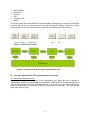
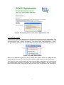
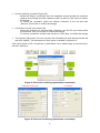
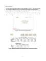
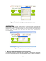
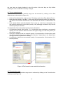
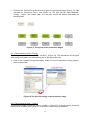
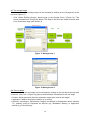
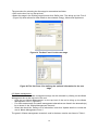
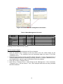
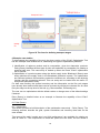
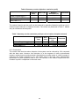
Manual
for the
CCaLC Optimisation Tool©
(Demo version)
October 2010
List of contents
1
2
3
4
5
6
6.1
6.2
6.3
7
7.1
7.2
8
8.1
8.2
System requirements ............................................................................................ 2
Tool development credits ...................................................................................... 2
Acknowledgements ............................................................................................... 2
Introduction ........................................................................................................... 2
CCaLC tool overview (CCaLC Optimisation tool - Demo)..................................... 2
Life cycle optimisation with demonstration case study.......................................... 3
Starting the optimisation tool ............................................................................... 3
Loading an analysis ............................................................................................ 4
Simplified procedure to optimise the existing system.......................................... 5
Reviewing the defined information of the life cycle optimisation ........................... 8
Optimisation details ............................................................................................. 8
System boundary ................................................................................................ 9
Reviewing the defined information in each life cycle stage ................................... 9
Raw materials stage.......................................................................................... 10
Production stage ............................................................................................... 10
8.2.1
Production stage – Energy ...................................................................... 11
8.2.2
Production stage – Output....................................................................... 11
8.3
Storage stage.................................................................................................... 13
8.4
Use stage .......................................................................................................... 13
8.5
Waste management .......................................................................................... 14
8.6
Transport stage ................................................................................................. 15
9
Example case studies ......................................................................................... 16
9.1
Paint (Demo) ..................................................................................................... 16
9.1.1
Introduction.............................................................................................. 16
9.1.2
Goal and scope of the study.................................................................... 17
9.1.3
Alternative description ............................................................................. 17
9.1.4
Impact assessment ................................................................................. 18
9.1.5
Conclusions............................................................................................. 20
Appendix A...................................................................................................................... 21
Appendix B...................................................................................................................... 22
Appendix C ..................................................................................................................... 22
1
1
System requirements
The CCaLC Optimisation Tool was designed and built using the English version of Microsoft
Excel 2003 and 2007 for Windows XP. It may not run properly on non-English operating
systems as well as on older versions of Excel or Windows. The tool is designed for use on
PCs and is not suitable for use on Mac computers.
Before using the tool, please ensure that Solver is loaded in Excel (see Appendix C).
This Demo version of the Optimisation tool is independent of the CCaLC Tool and can be
run without the need to download the CCaLC Tool first.
Please note that, depending on the speed of your computer, some operations may take
longer to complete. Normally, the hour-glass will indicate that the system is busy. If it
appears that there is no response after clicking on an option or action-button or the cursor
does not turn into the hour-glass, please wait a few seconds as the system is busy and may
take some time to complete the action.
2
Tool development credits
The CCaLC family of tools (CCaLC and CCaLC Optimisation) has been developed by a
research group based at the University of Manchester and led by Professor Adisa Azapagic.
The CCaLC Optimisation Tool was developed by Yu Rong. The following researchers were
also involved in the development of the CCaLC Optimisation tool:
 Haruna Gujba;
 Harish Jeswani; and
 Anthony Morgan.
For further information, contact: [email protected]
3
Acknowledgements
The CCaLC project was funded by the Carbon Trust, EPSRC and NERC (grant. No.
EP/F003501/1). Numerous industrial partners have contributed to the development of the
tool and their help is gratefully acknowledged. For more information visit www.ccalc.org.uk.
4
Introduction
The CCaLC Optimisation Tool has been developed to help minimise carbon footprints along
supply chains. In addition to carbon footprints, economic costs and profits can also be
optimised and the trade-offs between the carbon and costs/profits examined. Other
environmental impacts (e.g. human toxicity, acidification, eutrophication, etc.) as well as
process capacity can be included in optimisation as optional constraints.
The CCaLC Optimisation Tool works in conjunction with the CCaLC Tool. The CCaLC Tool
is used first to estimate a range of environmental impacts and value added along a supply
chain. The Optimisation tool can then be used to optimise on the carbon footprint or
costs/profits. However, for this Demo version of the tool, the Optimisation Tool can be used
without the CCaLC Tool.
5
CCaLC Optimisation Tool (Demo) overview
The tool has been developed in Microsoft Excel and is run by macros. The worksheets are
locked and are not accessible to the user. Information can be entered into the tool via user
forms that are activated by clicking buttons at the top of the worksheets and the relevant box
for each stage. The user can navigate around the tool using the links provided.
Figure 1 shows the top-level layout of the tool. This represents a map of a typical product
life-cycle and includes the following stages:
2






Raw materials;
Production;
Storage;
Use;
Transport; and
Waste.
The Excel menu bars and toolbars are largely disabled, although the in-built excel File/Save
functions can be used to save the tool at any point during the analysis. There are several
menus specific to the tool, the functions of which are described later in this manual.
Figure 1 Top-level view of the CCaLC Optimisation tool
6
Life cycle optimisation with a demonstration case study
6.1 Starting the optimisation tool
Figure 2 shows the opening screen of the optimisation tool. When the tool is opened, it
automatically checks whether the Solver is installed or linked properly. During this procedure,
the tool may reload the Solver (see Appendix B). In that case, the tool will be saved and
closed automatically (this operation may take a short time to complete). The user should
then open the tool again.
3
Figure 2 The opening screen of the CCaLC Optimisation Tool
6.2 Loading an analysis
There are two optimisation studies built in the demo version of the CCaLC Optimisation Tool
to demonstrate how the performance of a system can be optimised. On opening the tool, the
first case study (Paint – Demo) is loaded up. The second case study (Bioethanol – Demo)
can be loaded by clicking on the CF study menu item at the top of the screen (see Figure 3).
Figure 3 CF study menu options
Select Load optimisation study from the CF Study menu option. A form for loading the case
study pops up (Figure 4). The user can then select the study from the list and click ‘Load’.
This loads the base case study and the related specification for optimisation, as specified for
the demonstration purposes. To optimise the case study after loading it, the user needs to
click ‘Start Optimisation’ at the top of the top–level view. This is explained in the next section.
4
Figure 4 The form for loading a demonstration case study
Note:
 In the demonstration version of the optimisation tool, the functions of the rewriting, deleting
case study and starting new study are disabled. These are fully functional in the full version
of the tool.
6.3 Simplified procedure for optimising the existing case studies
To start optimisation, click on Define Optimisation Objective button on the top level of the
tool, as shown in Figure 5. For each demonstration case study, the user can carry
optimisation on one of the objective functions shown in Figure 5. Further constraints can also
be defined. The simplified optimisation procedure is describe below.
Step 1: Define the objective function by clicking ‘Define Optimisation Objective’ at the top of
the screen at the top level of the tool (Figure 5).
Figure 5 The form for defining objective functions in the optimisation
Step 2: Define the optimisation constraints by clicking ‘Start Optimisation’ at the top of the
screen to bring up the ‘Constraints in Optimisation’ form (Figures 6a & 6b), where the
optional constraints relevant to process capacity, economic and environmental impacts may
be defined.
5

Process capacity constraint (Figure 6a):
– Select the Stage in production from the dropdown list and provide the maximum
capacity for the stage and click ‘Update’ to add it to the list; Click ‘Next’ to confirm
the change.
– To delete the constraint, select the defined constraint in the list and click
‘Remove’; Click ‘Next’ to confirm the change.

Constraints over life cycle (Figure 6b):
– Select the economic or environmental constraint over the life cycle and provide
the maximum value Click ‘Next’ to confirm the change.
– To remove constraints, de-select the check box. Click ‘Next’ to confirm the change.

Tool Options (Figure 6b): The user may alter the information for each edit box on this tab
and click ‘Update’. The description for each option is detailed in Appendix A.
Click ‘Next’ button on the ‘Constraints in Optimisation’ form, which brings an overview form,
and click ‘Optimise’.
Figure 6a The form for defining optimisation constraint(s)
Figure 6b The form for defining optimisation constraint(s)
6
Step 3: Optimising…
 The Excel status bar shows progress during optimisation (Figure 7). This may take some
time. During the optimisation, the user can terminate the procedure by pressing ‘Esc’.
 When the Solver finds an optimum result, the message box shows ‘Done!’ and the button
‘View Optimisation Report’ is enabled. The optimisation results can then be accessed by
clicking on this button (examples shown in Figures 8 & 9).
 If the Solver cannot find a feasible solution, the message box shows ‘Tool did not find a
result.’. Click ‘Back to the top level’ at the top of the screen to go back and review the data
input or constraints.
Figure 7 The view during optimisation
Figure 8 Example results for an optimised study summarised in tables
7
Figure 9 Example results for an optimised study shown graphically
7
Reviewing the defined information of the life cycle optimisation
7.1 Optimisation details
The Optimisation details can be reviewed by clicking on the ‘Define Optimisation Detail’
button at the top of the screen at the top level of the tool. The user form is then activated as
shown in Figure 10. Note that in the Demo version of the tool, the information in this form is
locked. Click ‘Exit’ after reviewing.
The information includes:
1. The details of the functional unit used in optimisation. This is normally the same as the
name of the functional unit in the Base Case which is being optimised;
2. The units for mass, energy, distance and volume used in the optimisation;
3. The description of the optimisation problem:
• Optimisation category: this defines what the optimisation will be targeted at (for
example ‘Product for different use’ or ‘Various products for specified use’)
• ‘Format of the raw material quantity’: If Amount is selected, the unit of the raw
materials is ‘mass unit/functional unit’ (e.g. kg/ f.u.) and the quantity is a fixed number.
If Composition is selected, the unit of the raw materials is ‘% of product’ and quantity
is a fixed number. If Composition Range is selected, the unit of the raw materials is
‘% of product’ and the composition is set as variable in the optimisation (e.g. as in the
optimisation study case ‘Paint (Demo)’).
8
Figure 10 The form for defining/reviewing optimisation details
7.2 System boundary
Clicking on the System Boundary button brings up the form to view the product life cycle
stages included in the optimisation (see Figure 11). The life cycle stages considered in the
optimisation are shown on the right-hand side of the user form. In the demo version of the
tool these cannot be changed. In the full version, the stages can be selected and deselected as desired.
Figure 11 The optimisation boundary form
8
Reviewing the defined information in each life cycle stage
The information for each life cycle stage can be reviewed by clicking on the relevant life
cycle box on the top level of the tool. In the demonstration version of the tool, the buttons on
9
the user forms are largely disabled. In the full version of the tool, they are fully flexible
allowing the user to make the necessary changes.
8.1 The raw materials stage
The information on the raw materials stage can be reviewed by clicking on the Raw
Materials box at the top level (Figure 12).



Click the Raw Material box at the top level. This brings up the form Raw Material Form 1;
Select the raw material in List Box 1, which lists all raw materials used in the base case.
The defined raw material alternatives in the optimisation are shown in Alternative(s) list;
and
Click ‘Update Details’ and Raw Material Form 2 pops up. In this form, the details of the
raw materials alternatives include the quantity, cost, packaging and waste. Only the raw
material quantity is essential.
The expression of the raw material quantity in the optimisation:
 In Optimisation Details (See Section 7.1), if composition range is defined as raw material
quantity, the user needs to define the lower and upper range (% of the final product) for
the relevant material;
 If amount is defined as the raw material quantity, it is expressed as a fixed number (with
unit ‘Mass unit/ function unit’ or ‘Mass unit/unit product’, depending on the Optimisation
Category defined in Optimisation Details);
 If composition is defined as raw material quantity, it is expressed as a fixed number (% of
the final product).
Figure 12 The forms for raw materials information
8.2 The production stage
The information on the production stage can be reviewed by clicking on the Production box
at the top level (Figure 13).
10

Click the box ‘Production’ at the top level to go to the production stages (Figure 13). This
activates the Production Form 1 (see Figure 14). The form has the ‘Input Materials’,
‘Energy’, ‘Output’ and ‘Waste’ tabs. The user can review the defined information by
selecting tabs.
Figure 13 The layout of the production stages
8.2.1 The production stage – Energy
The energy options used are listed in List Box 1 (Figure 14). The alternatives for the base
case energy are listed in the alternative(s) list on the right-hand side.

Click on the ‘Update Energy Alternatives’ button to view the alternative energy options,
amounts and costs.
Figure 14 The form for energy in the production stage
8.2.2 The production stage – Output
The production stage outputs are listed in List Box 1 (Figure 15). In the full version of the tool,
these can be modified (see Figure 15); in the demo version they are disabled.
11
Figure 15 The form for the outputs in the production stage
For example, in ‘Paint (Demo)’, there are two alternative outputs: Market entry (Link with
material: pigment <30% of product) and High performance (When pigment >30% of product).
Note that the output cost is the selling price.
Packaging for the outputs can also be defined at this stage via the button ‘Define the
Packaging for Output’ (Figure 16). The packaging for the output is set as an associated
parameter which means it will be calculated with the associated output but not optimised.
Figure 16 The form for output packaging
12
8.3 The storage stage
The information on the storage stage can be reviewed by clicking on the Storage box at the
top level (Figure 17).
•
Click ‘Define Existing Storage’, which brings up the Storage Form 2 (Figure 18). This
shows information on Energy and Waste. The steps in this form are similar to those used
in the Production stage (see Section 8).
Figure 17 Storage form 1
Figure 18 Storage form 2
8.4 The use stage
The information on the use stage can be reviewed by clicking on the Use box at the top level
of the tool, Use Form 1 (Figure 19) pops up with the basic information for the use stage.
 Product: Which product(s) from the production stage is/are used in this stage?
 Application: What is the product used for (e.g. to eat)?
 Quantity: according to Optimisation Category as defined in Optimisation details (Section
7.1), quantity could be expressed as Amount (e.g. Bioethanol (Demo)) or Application
amount (e.g. Paint (Demo)).
13
The procedure for reviewing the Use stage is summarised as follow:
 Click on the box ‘Use’ on the top level;
 Select the stage in the Existing stage list and click ‘Define Use’. This brings up Use Form 2
(Figure 20) which allows for other details to be reviewed: Energy, Waste and Appliances.
Figure 19 The Use Form 1 for the use stage
Figure 20 The Use Form 2 for defining the optional information for the use
stage
8.5 Waste management
The information on the waste management stage can be reviewed by clicking on the Waste
Management box at the top level of the tool.
• Click the box ‘Waste Management’ on the top level of the tool to bring up the Waste
Management Form 1 (Figure 21);
• For each waste stream, the waste management alternatives are listed in the alternative(s)
list or shown in the ‘Waste Management Scenario’;
• Select the check box ‘Define cost of alternatives’ and click ‘Update details’ to review the
cost in Waste Management Form 2.
The generic ‘Waste management scenarios’ used in the demo version are shown in Table 1.
14
Figure 21 Forms for waste management information
Table 1 Waste Management Scenario
Materials
Recycling (%)
Landfill (%)
Incineration with energy recovery (%)
Aluminum
34.60
65.40
0.00
Steel
61.70
38.30
0.00
Paper/cardboard
79.80
16.20
4.00
Plastics
23.70
72.30
4.00
Glass
61.30
38.70
0.00
Wood
78.50
17.50
4.00
Source: Department of Environment Food and Rural Affairs (DEFRA), Making the most of packaging A strategy for a low-carbon economy (2009).
8.6 The transport stages
To review the transport steps between the life cycle stages:
 Click the relevant box ’Transport’ at the top level of the tool, which brings up the
‘Transport Form 1’. The materials from the associated stage are shown in List Box
‘Transport Form 1’.
 Select the target transport stage and Click ‘Define Transport’, to show ‘Transport Form 2’.
Transport alternatives can be viewed by selecting the item in ‘Transport Alternatives’ list.
In the optimisation, transport type and distance are set as variables.
 Click ‘Exit’ to leave ‘Transport Form 2’
 Click ‘Exit’ in ‘Transport Form 1’ which brings up the ‘Message box’. If ‘No’ is selected,
‘Transport Form 1’ will be closed. If ‘Yes’, then transport steps that are being reviewed
should be selected.
15
Transport Form 2
Transport Form 1
Figure 22 The form for defining transport stages
9 Example case studies
To demonstrate the capability of the tool, the demo version of the CCaLC Optimisation Tool
has two example case studies built in, addressing two types of optimisation problems:
i) Identification of optimum product and its composition, given the alternative products:
Paint (Demo) identifies the best type of paint and optimises its composition for painting a
specified wall area. This case study is loaded up when the Demo CCaLC optimisation
tool is opened.
ii) Optimisation of a product system along the whole supply chain: Bioethanol (Demo) case
study optimises the supply chain in the Bioethanol production system. The optimisation
tool chooses optimum raw materials, production conditions etc. according to the objective
function and the constraints selected. This can study can be loaded from the menu CF
study/Load optimisation study.
For both case studies, the system boundary and the information on the life cycle stages
have already been defined and these can be reviewed by clicking the relevant box for each
life cycle stage on the top level of the tool (e.g. Raw materials, Processing etc.).
The user can run optimisation with the default values or change some of the default settings
if desired.
Paint (Demo) is detailed below as an example to illustrate the capability of the CCaLC
Optimisation Tool.
9.1 Paint (Demo)
9.1.1 Introduction
This section provides a brief description of the optimisation case study – Paint (Demo). The
following sections describe the goal, system boundaries and inventory data used for the
case studies.
Two types of the paint (‘market entry’ and ‘high performance’) are available for painting an
area of 1000 m2. The components of these two paints are the same, but are mixed in
16
different proportions. This determines their performance, which is in turn determined by the
objective function(s) and constraints. For example, the objective function could be to
minimise the carbon footprint and/or costs, subject to the constraints on production
capacities and certain environmental impacts. The optimisation tool then chooses the best
type of paint and optimises its composition to satisfy the objective function and the
constraints.
9.1.2 Goal and scope of the study
Goal of the study: The main goal of this study is to answer the questions such as which paint
should be chosen for painting, what is the optimised composition for the chosen paint, which
alternatives should be used to substitute those in the existing study, what are the trade – offs
for other environmental impacts (e.g. human toxicity, acidification, eutrophication, etc) and
what is the optimised case.
Functional unit: The functional unit of this study is defined as ‘the amount of paint needed to
paint an area of 1000 m2’.
Scope and system boundary: The system boundaries are from ‘cradle to grave’. The life
cycle stages in this case study include:
 Raw materials and transport to the paint production site
 Paint production
 Paint storage
 Use of the paint
 Transport between the above stages and
 Waste management in the life cycle.
9.1.3 Description of alternatives
Raw materials: The alternatives defined in the raw materials (compositions as the
optimisation variables) are presented in Table 2.
Table 2 Raw materials
Raw materials
Quantity (% of the product)*
20 - 40 %
2 - 20 %
2 - 20 %
9.94 %
1.1 %
2.52 %
31.8 %
Pigment
Filler 1
Filler 2
Binder 1
Additive 1
Additive 2
Water
* ‘Composition Range’ is selected as ‘Format of the raw material quantity’ when defining the
optimisation details (described in Section 6.2), a default constraint is that the total raw material
quantity is 100%.
Table 3 Descriptions of the two paints
Alternative
product
Unit quantity
(kg/m2)
High
performance
0.1
1.5
Market entry
0.17
1.4
Costs
(GBP/kg)
Description of packaging
Output Packaging 1
[ Amount:4% of associated
product; Cost: 0.8 GBP/kg]
Output Packaging 2
[ Amount:5% of associated
product; Cost: 1 GBP/kg]
17
Link with Raw
material*
Pigment > 30%
Pigment < 30%
* ‘Link with Raw material’ is an optional constraint in the optimisation procedure, which can
be defined in the production stage.
Energy: The energy alternatives for heat and electricity are presented in Tables 4&5.
In the production process, energy consumption is defined with a unit of ‘kWh/ kg product’ in
this study. With different paint generation, the energy amount is calculated by the tool.
In the ‘storage’ and ‘use’ stages, the energy is defined as associated alternative, which links
with the input material. As presented in Table 5, the alternatives for high performance and
market entry are different.
Table 4 Energy alternatives in the production stage
Energy (Base Case)
Energy alternatives (Optimisation
Case)
Quantity (kWh/kg product)
Electricity - EU grid
0.03
Electricity from heavy fuel Oil
0.04
Electricity - EU grid
Table 5 Energy alternatives in the storage stage and use stage
Energy (Base
Case)
Electricity - UK grid
Energy alternatives
(Optimisation Case)
Storage stage
Electricity from heavy fuel
Oil
Electricity - UK grid
Heat from heavy fuel
oil
Energy Group 1
Energy Group 1
Energy Group 1
Quantity
(kWh/kg)
0.008
0.008
Heat from heavy fuel oil
0.01
Heat from natural gas
0.02
Electricity - UK grid
0.011
Electricity from hydro
0.014
Use stage
Electricity - EU grid
Electricity - France grid
Electricity from natural
Electricity from hydro
Link with
0.3
0.6
0.3
0.2
Market entry
High
performance
Market entry
High
performance
Waste Management and Transport: The transport distances and the transport types are
defined as the optimisation variables for the Transport stage, which can be reviewed by
clicking the relative boxes in the worksheet. In the Waste Management phase, the
optimisation variables are the alternative methods for each waste stream.
9.1.4 Impact assessment
With the objective of minimising carbon footprint, the results of Paint (Demo) as optimised in
the tool are shown in Figure 23. High performance (one of the paint alternatives) is chosen
as the optimum paint. The optimised carbon footprint is 192.6 kg CO2 eq. per 1000 m2 of
painted area. Compared with the Base Case, the carbon footprint is reduced by 32%.
18
However, this results in 4% increase in the human toxicity potential from the Base Case, as
shown in Figure 24.
Carbon Footprint
3.00E+02
2.50E+02
CO2 eq./ f.u.
2.00E+02
1.50E+02
1.00E+02
T
ot
al
T
ra
ns
po
rt
S
to
ra
ge
W
a
st
e
R
aw
P
ro
du
ct
io
n
m
at
e
ria
ls
0.00E+00
-5.00E+01
U
se
m
a
na
ge
m
en
t
5.00E+01
Optimisation study
Life cycle s tage
Base case
Figure 23 Carbon footprint for the optimised case compared with the base case
Human Toxicity Potential
100.00
DCB eq./ f.u.
80.00
60.00
40.00
20.00
Life cycle s tage
T
ot
al
Tr
a
ns
po
rt
S
to
ra
ge
U
se
m
a
na
ge
m
en
t
W
a
st
e
R
aw
-20.00
P
ro
du
ct
io
n
m
at
e
ria
ls
0.00
Optimisation study
Base case
Figure 24 Human toxicity potential for the optimised case compared with the base
case
With a different objective function, for example, ‘Maximise profit’ (the difference between the
selling price and operating costs), a different optimised case can be obtained. Market entry
is now chosen as the best alternative, because more of this type of paint is needed to cover
the same area, which results in the higher total profit. However, the carbon footprint
increases significantly compared to the previous optimisation case or even with the base
case, as shown in Table 6.
19
Table 6 Summary results (objective: maximise profit)
Carbon Footprint kg/f.u.)
Optimum
Case
336.71
283.17
Relative
Difference (%)
18.91
Base Case
Comments
Increase
Operating Costs (GBP/ f.u.)
96.78
65.86
46.95
Increase
Profit (GBP/ f.u.)
141.22
85.00
66.14
Increase
The carbon footprint and the profit can be balanced by selecting ‘Maximise profit per unit of
carbon footprint reduced’ as objective function. The results are presented in Table 7. Market
entry is selected as the best paint.
Table 7 Summary results (maximise profit per unit of carbon footprint reduced)
Relative
Difference Comments
(%)
258.57 283.17
8.69
Reduction
108.73
65.86
65.09
Increase
129.27
85.00
52.08
Increase
Optimum
Case
Carbon Footprint kg/ f.u.)
Operating Costs (GBP/ f.u.)
Profit (GBP/ f.u.)
Base
Case
9.1.5 Conclusions
The results show that the carbon footprint of the system can be reduced by 32% compared
with the base case. However, this reduction is at the expense of other environmental
impacts, notably human toxicity potential. Optimisation on profits results in a 66% increase of
profit but the carbon footprint is now 19% higher than in the base case. Simultaneous
optimisation on both objectives leads to an 8.7% reduction in the carbon footprint and 52%
increase in profit in comparison to the base case.
20
Appendix A: Tool options
The user can control several options used by the optimiser through the Tool Options tab on
Constraints in Optimisation form (Figure A.1).
Figure A.1 Tab for tool options
Max Time: The maximum amount of time (in seconds) will spend solving the problem. The
value must be a positive integer. The default value in the tool 3000 is adequate for most
small problems, but you can enter a value as high as 32767.
Iteration: The maximum number of iterations use in solving the problem. The value must be
a positive integer. The default value 3000 is adequate for most small problems, but you can
enter a value as high as 32767.
Precision: A number between 0 and 1 that specifies the degree of precision to be used in
solving the problem. The default precision is 0.000001. A smaller number of decimal places
(for example, 0.0001) indicate a lower degree of precision. In general, the higher the degree
of precision you specify (the smaller the number), the more time tool will take to reach
solutions.
Tolerance: A decimal number between 0 and 1 that specifies the degree of integer
tolerance. This argument applies only if integer constraints have been defined. You can
adjust the tolerance value, which represents the percentage of error allowed in the optimal
solution when an integer constraint is used on any element of the problem. A higher degree
of tolerance (allowable percentage of error) might speed up the solution process.
Convergence: A number between 0 and 1 that specifies the degree of convergence
tolerance for the nonlinear problem. When the relative change in the target cell value is less
than this tolerance for the last five iterations, the optimisation converges to a solution.
21
Appendix B: Load the Solver Add-in by the tool
The tool automatically checks if the Solver is loaded properly when the users open it. If the
Solver was not added into this tool properly, the tool will reload it (Message: as shown in
Figure B.1). To confirm this reloadiing, the tool will be saved and closed automatically; this
operation may take longer time to complete. Then open the tool again.
Figure B.1
Appendix C: Load the Solver Add-in in a new workbook
•
In Microsoft Office Excel 2007
1. Open Microsoft Office Excel 2007;
Click the Office Button ;
Click Excel Options (Bottom right);
Click Add-Ins;
Click Go. (Bottom middle);
Check the box for Solver Add-In;
If Solver Add-In is not listed, use Browse… to locate ‘SOLVER.xlam’ in the
application file (e.g. C:\Program Files\Microsoft Office\ OFFICE12\ Library\
SOLVER\ SOLVER.xlam); and
8. Click OK.
If prompted that Solver is not installed, click ‘Yes’ to install. Insert the install media if
prompted.
2.
3.
4.
5.
6.
7.
•
In Microsoft Office Excel 2003
1. Open Microsoft Office Excel 2003;
2. Click the Tools on the top menu;
3. Click Add-Ins;
4. If Solver Add-In is not listed, use Browse… to locate ‘SOLVER.xla’ in the
application file (e.g. C:\Program Files\Microsoft Office\OFFICE11\ Library\
SOLVER\ SOLVER.xla);
5. Check the box for Solver Add-In; and
6. Click OK.
22