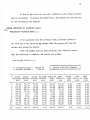
Download SR41/B This document is not a departmental publication. User`s

ENERPUB
User's Manual
November 1982
Assistance and Information:
K. Ford
Design Aids Engineer
Solar Programs Office
Sir Charles Tupper Building
Riverside Drive
Ottawa K1A OM2
(613) 998-3641
This document is not a departmental publication.
Do not cite as a reference or catalogue in a library,
SR41/B
User Responsibility
Users are responsible for the validity of the information generated by the
ENERPUB program.
Consequently the program should not be used by those who do
not comprehend the technical field to which this program applies.
Neither
Public Works Canada nor any person acting on behalf of the department makes any
warrenty or assumes any responsibility for accuracy, completeness or usefulness
of any information generated by this program.
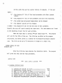
TABLE OF CONTENTS
LIST OF FIGURES
Page
FIGURE 1:
Solar Heating System Schematic - No Heat Pump - system type 0
3
FIGURE 2:
Solar Heating System Schematic - Heat Pump in Series with
Solar Supply - system type 1
4
FIGURE 3:
Solar Heating System Schematic - Heat Pump in Parallel with
Solar Supply - system type 2
5
FIGURE 4:
Solar Heating System Schematic - Heat Pump Supply Only system type 3
6
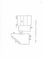
FIGURE 5:
Oil Tank Heating System - system type 4
7
FIGURE 6:
ENERPUB Flow Chart
FIGURE 7: · ENERPUB Program Structure
40
59
I
I
I
I
I
I
I
I
I
I
I
I
I
I
I
I
1
1.
INTRODUCTION
The ENERPUB computer program,developed by Enermodal Engineering
Limited for Public Works Canada,can be used to simulate the performance of
liquid-basedseasonalorshort-term storage solar space heating systems with
or without a heat pump.
The program can also simulate the performance of
a solar heating system used to heat oil in oil storage tanks.
ENERPUB is
not suitable for simulation of solar domestic hot water systems specifically
because of the restrictive heat exchanger models.
The ENERPUB program has many advantages over other solar simulation
programs.
Because performance calculations are made for each simulated hour,
the program results are potentially more accurate than those of programs
using a monthly calculation procedure, such as FCHART.
In addition, the
ENERPUB program can simulate a wider range of parameters than programs restricted
by monthly average correlation equations.
Several of the models in the
ENERPUB program were adapted from WATSUN models (WATSUN is an hour-by-hour
computer program developed by the University of Waterloo).
ENERPUB has
several enhancements over the WATSUN space heating programs:
1) Stratified tank model for short term or seasonal storage.
2)
Four possible heat pump locations.
3)
Inclusion of heat loss from the storage to the building, outdoors
or ground.
4)
Inclusion of heat loss from collector and storage piping to the
building, outdoors or ground.
The ENERPUB computer program gives detailed and accurate results for
liquid-based seasonal or short-term storage provided that reasonable values
for all system parameters are input.
this manual before using the program.
All users should read and understand
2
2.
THE ENERPUB COMPUTER PROGRAM
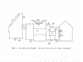
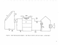
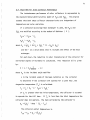
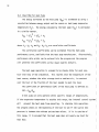
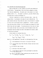
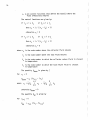
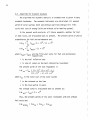
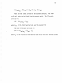
2.1 System Configurations
Figures 1-4 show the four possible space heating systems that can be
simulated by the program.
The difference between these systems is the manner
in which the heat is delivered to the space heating load.
oil tank heating system.
Note that these systems are all liquid-based; the
program cannot handle air-based systems.
Piping heat losses can be considered
for each of the four regions shown on the figures:
building supply and return.
collector supply and return,
The abbreviations used in the figures are:
CL
- solar collector
ST
- thermal storage tank
OIL
- oil storage tank
AUX
- auxiliary heating system
DHW
- domestic hot water system
HP
- heat pump
HXc
- collector-storage heat exchanger
HXW
- storage-DHW heat exchanger
HX 8
- storage-building heat exchanger
P1,P2,P3,P4
- circulation pumps
V1,V2,V3,V4
- control valves
@,@,G),(D -
Figure 5 shows the
piping heat loss regions
2.2 System Operating Strategies - Space Heating
The operating strategy for the four space heating systems can be
broken into three distinct steps:
domestic hot water (DHW) heating.
solar energy collection, space heating and
(1)
OHW
HXW
1
ST
2
0
HXc
Node 3
Node N
P1
®
P2
Figure 1:
G)
Solar Heating System Schematic - No Heat Pump - system type 0
w
..,.
CD
DHW
HXc
ret
----------- --
I
I
0
P3
HX
w
v1
1
ST
----------- -
P1
®
I v~
,
,
YV4
HP
V2
P2
P4
0
Figure 2:. Solar Heating System Schematic - Heat Pump in Series with Solar Supply - system type 1
--2::--
~~-
CD
DHW
0
HXw
Hx,
ST
P3
HX
P1
Figure 3:
®
P2
HP
8
0
Solar Heating System Schematic - Heat Pump in Parallel with Solar Supply - system type 2
(J1
a-
Ci)
DHW
HXw
P3
-.
G)
HXc
ST
HP
HX 8
P1
®
P2
P4
0
Figure 4:
Solar Heating System Schematic - Heat Pump Supply Only - system type 3
~-
7
....
-0
_J
Q)
c.
>.
...,
E
...,
Q)
Vl
>.
Vl
C\1
a..
E
...,
Q)
Vl
>.
V)
en
...,"'
·~
8
X
u
"'
Q)
~
:I:
-""
e
a..
"'"'
f-
~
·~
0
..
L()
Q)
'en
"'
·~
LL.
8
2.2.1 Solar Energy Collection Strategy
If the collector inlet fluid temperature is lower than the average
collector plate temperature, solar energy can be collected and transferred to
the storage tank.
If the collector outlet temperature approaches the boiling
point, the system will not operate.
In this case, either the collectors would
be drained or solar energy dumped through the pressure relief valve.
2.2.2 DHW Heating Strategy
Domestic hot water preheating is accomplished by passing city mains
water through a heat exchanger contained in the top of the storage tank.
The
water, if not warmed to the desired water temperature, is heated by the
conventional water heater.
Note that the heat exchanger only operates when
there is a water demand, i.e. there is no recirculation of the water.
If the
DHW heating load forms a large portion of the total heating load (greater than
20%) this model is not suitable and will not provide satisfactory results.
2.2.3 Space Heating Strategies
2.2.3.1 Space Heating Strategy - system type 0
No heat pump is used in this system.
If the building requires heat,
water from the storage tank is circulated through the building heat exchanger.
This heat exchanger may be either hot water radiators or a water-to-air heat
exchanger placed in the furnace return air duct.
If the solar heat cannot meet
the building demand, the auxiliary heater will make up the difference.
2.2.3.2 Space Heating Strategy - system type 1
This system is similar to system type 0 except that a heat pump is
9
added.
The system first attempts to meet the heating demand from the solar
heat (valves 1 and 2 open, valves 3 and 4 closed).
If the solar heat cannot meet
the demand, the solar heating system will not operate, and the heat pump will
attempt to meet the load using the storage tank as the heat source (valves 3 and
4 open, valves 1 and 2 closed).
If the heat pump cannot meet the demand, the
auxiliary unit will make up the difference.
2.2.3.3 Space Heating Strategy - system type 2
This system operates in the same manner as system type 0 except that a
heat pump is used as an auxiliary heater with the outside air as the heat source.
If the solar heat cannot meet the demand, the heat pump will come on.
Note that
unlike system type 1, the heat pump and the solar heat can supply heat to the
building at the same time.
If the two heat sources cannot meet the heating demand
the auxiliary unit will make up the difference.
2.2.3.4 Space Heating Strategy - system type 3
This system is similar to system type 1 except that solar heat cannot be
delivered directly to the heating load the solar heat is always transferred to
the load by means of the heat pump.
This system will always have poorer performance
than system type 1, however, it has a simpler layout and control strategy.
2.3 System Operating Strategies - Oil Tank Heating
This system differs from the previous four in that there is no space
heating load.
The heating requirement is to keep the oil above a minimum temperature
(to prevent excessive viscosity) so that it can be pumped out when necessary.
The control strategy for heat collection is as described in Section 2.2.
There is no DHW heating in this system.
As will be described in Section 3.1
10
the DHW input parameters can be used to simulate draws of oil. There is no
control strategy for space heating; the collected heat is continually added
to the. tank.
2.4 Tutorial Session
This section describes the use of the ENERPUB computer program.
A full
description of the input parameters is given in Section 3, and program output
is described in Section 4.
When you have successfully signed on to your account and accessed the
program, the computer will respond with the header.
************************************
*
*
*
*
*
*
ENEilPUB - 1
*
*
*
*
*
*
*
*
PROGRA!I VERSION 1. 2
*
*
* ENERMODA~ ENGINEERING LIMITED *
JULY 1982
*
*
*
*
*
*
*
*
************************************
DEVELOPED BY:
ENEilMODAL ENGINEERING LIMITED
421 KING STREET NO&TH
WATERLOO, ONTARIO N2J 4E4
(5191 884-6421
**
LIQUID BASED SOLAR HEATING SYSTEM **
WITH HEAT PUMP AND STRATIFIED TANK
I
;,
11
The program will prompt the user for system characteristics concerning
system type and whether the pipes or tank are buried.
ENTER
0 1
2
3
4
0
SOLAR SYSTEM TYPE ••••
STANDARD SOLAR SPACE HEATING (NO HEAT PUMP)
HEAT PUMP IN SERIES WITH SOLAR SUPPLY
HEAT PUMP IN PARALLEL WITH SOLAR SUPPLY
SOLAR ASSISTED HEAT PUMP ONLY
OIL TANK HEATING (NO HEAT PUMP)
DO IOU WISH ECONOMIC ANALYSIS ? (Y/N)
y
lBB THE PIPES OR TANK BURIED 1
(T/N)
The program will then print the message.
INSTRUCTIONS ••••
L - TO OBTAIN DATA LISTING
R - TO RUN PROGRAM (iiTH LISTING)
C - TO CHANGE SYSTEM TYPE
S- TO STOP SESSlOI. 0& •••
TO CBAIGE PlRAMETIR 1 TIPI CODE lUMBER
12
At this point the user has several choices of commands.
If the user
types •.•
"L" - the program will 1i st a11 the input parameters with their present
values.
"R" - the program will list all the parameters and start the simulation.
"C" - the system type and ground temperatures can be changed.
"S" - the computer session will be stopped.
a number - the program will ask for the new value of this parameter.
Normally the user will want to modify the input data.
The code numbers are listed
at the beginning of each line for each variable.
When the input data is correct, the user should type "R". The program
will ask for the title of the run.
The title has no effect on the program
calculation, but merely serves as a method for distinguishing between computer
runs.
The title can be up to 72 characters in length on a single line.
fNTfR TITLE OF RUN
sa11ple run
After the title has been entered, the simulation starts.
The program
will print the title and the input parameters.
3AMPLE EUN
***
*
DATA lNFLT LISTING
***
GENERAL SYSTEM DATA
1.
2.
3.
4.
5.
6.
7.
1970
SIMULATION BEGINS IN YEAR ••••••••••••••••••
365
SIMULATION PERIOD (DAYS)•••••••••••••••••••
1
DA-11 CF THE PESlJD (1-365) •••••••• •••••••••
DETAILED Pill NT-OUT (NO=O, YES=I-Hh INTEEVAl)
0
STARTING HCUR CF FRINT INTERVAL (O, •• ,I) •••
0
TILTED ANGL.i:: Cf CCLLECTOiJ. (J:EGREES) -••••••• 55.00
COLLECTOR ORIENTATION (SCUTH=O. ,DEGREES) ••• o.oo
13
1 o. Gi,GSS CCi.LEL:Ci- hFi:;t<. (t:~) . . . . . . . . . . . . . . . . . . . . . 100.00
11. M~h.i~iUt': ~C.LLi:C'lQj I.JU~i.~l ·J.:Lol•l?. {C) ••••••••••
1. 7
1~. BLVU2.i\.c.D C..C.i.L-::·rcr:~GL. ~L.'\~1:. L:r F~hl:r.C~ (L:).
c.
13. PCAi.r. CF i?li<12S 1:;2 I <.:C1L:.C.1u,. ;..~,;.!. (•/!'1~).
60.
14. FlOW ha1~
Hi.CAP~~ll~ (~/&~-~>····•••••••
15. Fli-IAU-~LPHA (~CJUSlEU) ••••••••••••••••••• • 0.710
*
16. FR-UL (AuJuS~Et)
(o;M~-C) •• ••·•••••••••••• 3.910
17. BO, CGLFF. F0~ ll~CIDE~l ~hGL~ hU~ifi~~ ••••• -0.100
16. CO~L~~~C~-S~~aBGL iiX ~~iiLTiV~~~~~•••••••-·• 1.000
~U.
~ 1.
SJ..O~t-.Gi VCLUhi/CJLi.. rl..t.~:.~
(MJ/~·J2)
;;.Ti-.h!:.i..~"G ~.L.~J.r.;..~A:.U~i.i:.
(.:) ••••••• ••
4:- ....
SUJii,OUL~I:.-hG
25.
~t.
~7.
*
u.u75
••••••••••
~u.
~£r:F:::F.bl'Un:::
23. ICi' hlA'i LCSS CC.:..FF.
~4.
•• •• ••• •••
(\..) ••••••••••••••••
(11;·~) •••••••••••••••••
SlL.2.. bi.h.1 i.CS~) CC:.l-F .. (~;;c) ........... ••••••
BCIILL'l iJ.::.;..: .~,.,_,55 CUi-:Fi. (W/C) ••••••••••••••
• OF S~EnTltl~~i-Ct 1~~h S~G~~~i~ ••••••••••
*
*
~b.
SiG.
SlG.
.(.9.
i•Ji.N1~~UU
fJ~
C0Lli:I0R
}0~
EuilL~~G
r.L"'"'(.;idd~l-~
~~iU~b
rL~U~~
SlUbnG1
I~~o
~~~u
i~•d ......
.
~h~h •••••••
Ii.~·lt-. (-:) •••••••••
().00
o.oo
o.oo
1
1
1
4. (} 0
I:IEA'I fUl'!P DATA
30. lOiiER L.Hll'i OF EV APOliA1CR TEMP. (C).........
31. I:IIGHZli LI~I'I 01 EVAPOhATOli TEMP.(C) ••••••••
32. COEFFICIENiS CQ, CP OF HEAT PUMP :
5.000
ij48.000 15473.000
0.000
103.00C 5767.000
*
c.: a
20.0
0. 0
35.0
BUILDING DATA
40.
41.
42.
43.
44.
45.
4E.
BUILDING UA COEFF. (w/C) ••••••••••••••••••• 1000.0
POWER FOR HEATING FAN (Ji) •••••••••••• ••••••
0.
STORAGE-BUILDING EX EFFECTIVENESS •••••••••• 0.700
MIN.CAFACIIANCE RATE Of lOAD HX.(w/C) •••••• 3000.
DIRECT SOlAi GAI. FACTOi (M2)•••••••••••••• 0.00
INDOOR DESIGN 'IEMF~EATURE (C) •••••••••••••• 20.00
IN'IERNAL HOURLY HEAT G4IN SCHEDULE (KJ)
o.
o.
o.
o.
o.
1800.
3600.
2700.
54004500.
1800.
3600.
4500.
3600.
2700.
2700.
1dCO. 16200.
6300.
~700.
2700.
2700.
1800.
1800.
14
*
WA1ER LOAD DATA
so.
(C) . . . . . . . . . . . . . . .
TEMPERATURE
MAIN
liA'i:ER
51. DESIRED H01 WA lEE TEMP.
(C) •• ••••••••• • ••
52. DHil HX EiFEC!iVENESS •••••••••••••••••••••••
(LIT RES)
53. HOURLY H01 ii A:rER SCHEDUlE
o.
o.
o.
o.
o.
o.
o.
o.
*
o.
o.
o.
o.
o.
0.
o.
o.
o.
o.
o.
o.
6.00
40.00
50
o.
o.
o.
o.
o.
PIPING I:ATA
PIPE HEAT LOSS COHF - CCL R:<:;TU liN IIi/C)....
T:<:;MFEBATURE - COL F.ETURN (C)...
COEFF- COL SUPPL¥ (ii/C) ••••
LOSS
62. PIPE HEAT
- CCL SUPPlY (C)...
1EMPEiiA1URE
SURROUNDING
63.
64. PIPE HEAT LOSS CCEFF - Er:G SUPPLY (ii/C)....
65. SU!iROUNDING TEMPERATUi<E - ilDG SUPPlY (C) •••
66. PIPE HEAT LOSS CCEFF - Er:G E:STURN (ii/C) ••••
67. SURROUNDING TEMPEEATUEE- BLG RETURN (C) •••
6 0.
61.
7C •
SURROU~LING
.3Y~'.IJ4i~
0. 00
20.0
0.00
20.0
0.00
20.0
0.00
20.0
~_;_f.:.
L.J
(Yiii.:.\3) •••• •••••••• • • • • • • • • • • • •
~0
(YEA[~).......................
.ihl~.::.r.s~ t.A:.&.L CF i.Od~ (A} ................... 1v.ovo
i:,?.TL. Gi' !'.~IUB£~ (.:J:S~':;Ut-.:i i:\A'J:.~..) (:~o) ••••••••• 1V.IJ"J
a3U.
F!XiC ~C~i CE 5Glha CO~~v~~~i5 (~) •••••••••
FIX.:.;:; CC;;;. Cl !Ji:;.T PUMl- (.j.) •••••••••• •••••• .:160.
50.
Yi:rlC;J.Y h.'-1...~.. t~~·E!~r.t~Ct. CCST l.f' SuLt:.~\ CCME .. (*'/Y)
50.
Y"!lni..¥ i•lnlli1r.NAhCi:. cos~· Or IH·. (i/Yb)......
0.
SALVAGi.. Vai..U~ AT !NL Of f-~iCD (•).........
:z~o ..
u~~I'I .:~~si ur (:llll~TC:i.\ (~/1',2.) .......... ••••••
1.<:2.
Ui,ll: lOS I' Gt ::ilOnAGi. (£;t·i.i) •••••• •• ••••••••
71. Ii~~ OF ~~Al~
7L. •
73.
74.
75.
7o.
77.
76.
7~.
tlO.
a1. U~ll CC3l Of fGr.l AI ~~t::ii.NT (•/GJ) •••••••• 10.00U
8~ .. ~ ~~FLnliC~ ~A~E CF ~~~hGY!
1j.Q
1j.U
13.0
1j.u
13.u
1C.O
10.U
10.0
10.0
10.0
10.0
1u.u
1u.u
1J.u
1u.J
1u.o
10.0
10.0
10.0
10.0
15
If this is the first run, the solar radiation on the tilted collector
must be calculated.
To process the weather data, the program will ask the user
for the latitude of the location.
EliTER LATITUDE OF LOCATION (Di:G.)
45.
PROCESSIHG WEATHiR DlTJ. •••••
If on successive runs the collector slope, collector azimuth or
the first day of the period do not change, then the program will skip the
weather data processing section.
After the weather data has been processed, the simulation starts.
When the simulation is complete, the results are printed.
SiMULATION STARTS •••••
*
*
COLLECTOR AREA :
STC£AGE VOLUME :
1 00.00 M2
7.50 M3
*****************************
*
ENLRGY ANALYSIS SUMMARY
*
*****************************
--·
------·------·-------·-------·-------·-------·------·----·--·-------·rUMP
AUX.
wATER
SOLAR HT PUMP SPACE HT AUX.
SOLAR
M SOLAR
INCiDENT
COL~ECT
DELIVIR BhLIVER
(GJ)
(GJ)
(GJ)
33.15
62.33
53.94
53.14
56.93
52.65
52.87
40.89
30.88
24.25
25.61
13.27
28.34
13.30
27.95
24.99
15.31
7.55
5.14
8.16
10.72
14.64
10.55
10.66
(GJ)
SPACE HT
LOAB
(GJ)
(GJ)
(GJ)
65.34
61.99
42.07
19.11
7.55
5.14
8.40
10.72
24.83
51.11
69.63
52.04
34.04
17.07
3.81
0.00
o.oo
0.23
o.oo
10.19
40.56
58.56
LOAD
WATER HT PCwEh
(GJ)
(GJ)
---·-------+
·-------·-------+-------·-------·--------·-----·--·-------·0.00
0.00
O.GO
70.20
86.07
0.00
15.87
15.91
38.94
1
2
3
4
5
6
7
8
9
10
11
12
24.~3
17.34
7.73
4.81
7.48
10.64
13.43
10.41
10.70
o.oo
o.oo
o.oo
o.oo
O.JO
o.oo
o.oo
0.00
o.oo
o.oo
o.oo
0.00
o.oo
o.oo
o.oo
0.00
0.00
0.00
0.00
0.00
0.00
0.00
0.00
o.oo
0.00
o.oo
0.00
0.00
0.00
o.oo
0.00
o.oo
o.oo
o.oo
o.oo
o.oo
0.00
0.00
0.00
0.00
o.oo
0.00
0.00
o.oo
+
-----+-------+-------+-------+-------+-------+-------+----+--+-------+
0.0
0.0
0.0
287.1
451.9
0.0
164.8
164.9
525.6
YR
+--+-------+-------+-------+-------+-------+-------+-------+-------+-------+
16
**
TCTAL ENBiGY INPUT TC ELECTRIC RESISTANCE REfERENCE
OVER SIMULATION PERICE, GJ : 451.449
**
**
**
ENERGY SAVING:
SEASONAL PERFORMANCE FACTOR :
**
EN£RGY GAINED BY SlOB AGE TANK (GJ):
3E.41 PEhCENT
1.57
MAX. HOURLY ENERGY INPUT (MJ):
***
179.447
O. 036
ECONOr.IC ANAlYSIS
**
PliES.<; NT WO.iiTH (AUXIliARY ENEliGY .iNCL.)
(.1.UXHIAEY ENEi'lGY NOT INCL.)
**
LIFE-CYCLE UNIT CCS'I (LUC), .ii/GJ :
••
SCIA.ii lUC
1
$jGJ
SYSTE~
,
($):
($):
***
921514. b3
27776.34
1 o. 2 57
8.450
TO CHANGE PARAMETER, TYPE CCEE NUMBEli
s
The program will return with the prompt "TO CHANGE PARAMETER, TYPE
CODE NUMBER".
If the user is finished, type "S" to stop, otherwise modify
the input parameters as necessary and re-run the program.
The simulation procedure for an oil tank heating system is shown below.
The user should take note of the parameters that should be modified.
ENTER SOLAR SYSTEM TYPE ••••
0 - STANDARD SOLAR SPACE HEATING (NO HEAT PUMP)
1
HEAT PUMP IN SERIES WITH SOLAR SUPPLY
2
HEAT PUMP IN PARALLEL WITH SOLAR SUPPLY
3
SOLAR ASSISTED HEAl PUMP ONLY
4
OIL TANK HEATING (NO HEAT PUMP)
4
DO YOU WISH ECONOMIC ANALYSIS 1
(Y/N)
n
ARE THE PIPES OR TANK BURIED ?
n
INSTRUCTIONS ••••
(Y/M)
17
L - TO
R - TO
C - TO
S- TO
TO CHANGE
OBTAIN DATA LISTING
RUN PROGRAM (WITH LISTING)
CHANGE SYSTEM TYPE
STOP SESSION, OR •••
RARAMETER, TYPE CODE NUMBER
11
ENTER NEW VALUE OP PARAMETER
11
55
70 CHANGE PARAMETER, TYPE CODE NUMBER
51
ENTER NEW VALUE OP PARAMETER
51
55
TO CHANGE PARAMETER, TYPE CODE NUMBER
20
ENTER NEW VALUE OF PARAMETER
20
5.
TO CHANGE
PABAM~TER,
TYPE CODE NUMBER
22
ENTER NEil VALUE Ozc PABAMEiER 22
-100
TO CHANGE PARAMETER, TYPE CODE NUMBER
23
ENTER NEi VALUE OF PARAMETER 23
300
TO CHANGE PARAMETER, TYPE CODE NUMBER
24
ENTER NEW VALUE OF PARAMETER
24
600
TO CHANGE PARAMETER, TIPE CODE NUMBER
25
ENTER NEW VALUE OF PARAMETER 25
300
TO CHANGE PARAMETER, TYPE CODE NUMBER
53
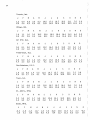
ENTER 24 VALUES OF HOI iiA1ER LOAD (LITRES)
0 0 0 0 0 0 0 0 0 100 100 200 200 200 200 100 100 100 100 0 0 0 0 0
10 CHANGE PARAMETER, TYPE CODE NUMBER
29
ENTER NEi VALUE OF PARAMETER
29
28
TO CHANGE PARAMETER, TYPE CODE NUMBER
21
ENTER NEW VALUE OF PARAIIE1EB
21
28
70 CHANGE PABAIIETER, TYPE CODE NUMBER
50
ENTER NEW VALUE OF PABAIIETER
50
28
TO CHAWGE PABl!IBtBR, tYPE CODE MUIIBBR
ENTER TITLE OP BOH
sample run 12
1
18
SASP LE IIU II 12
***
~NED~ L~SIING
tA!h
***
1970
365
1
1. sr~ULh~=u~ ti~GlNS I~ YLA~ ••••••••••••••••••
2. SIMU~h1:0b PL~lC~ (:AY5) •••••••••••••••••••
3. JAY1 Cf l'H.:. fLb.J..GC (1-JoS) •••••••••••••••••
4. D.t.'I.;.:..L.ED -1"'.:-.:fll'I-GUi {l:~C-=Ll,YL~=:.:-H;:.. :il~Ii~VAL)
S•
6.
7•
.::Jl.Ai-~i'~1~G
HCU£: CF P!\Ihl il·~':.'.ui1Yhi.. (t.J, •• ,Ij •••
J..l:l..T ... ~ tL~G:.L Oi' CCiLI:.C'~Ci~ .. (I:i..Gt.E~S) •• ••• ·••
..:.:OLi..w~1.(.=\ vnll.l\'Li.·~.J..JN (SDU'J:'h=0. ,ui(;f.i.~S) •••
10.
~dO~~
11.
bi1.A.:Lt'lU~~ CCill.CIC~ C.Ul1...Ll: 'iLi·~e. (C) ... •• ••• •••
C0~liC1C~
A~LL
0
0
55.00
o.oo
(~2)
•••••••••••••••••• 100.00
55.
1~. ~~~UihiC ~OL~-SiC~AG~ l~MP. ~iFfL~i~~i (C).
1.70
13. ~C•LA Of ruci~S 1~2 1 Cci~LClCa Ad~~ (~/cl~).
0.
14. t,1C- A~'.i.C: * l!I.<..af.,.Cllj, 'f. (w/ri~-C.:) ••••• •••• ••
60.
15. FR-Tr.U-ALPHA (ADJU.)l i.D) ••••••••••••••••• ••• 0. 710
1
16. fit·UL
3.91
(W/112-C) •••••••••••••••••
(ADJOSit.L)
CC~Ff. FOR INCIDENT A~Glj hODiflth ••••• -0.100
CCLiL~lC~-S~O~bGE HX iff~CliV2~iSS ••••• 4 • • • 1.000
17. EO,
16.
*
bl'C!iAGi i;rilA
(l'ij/~12} •••••••• ·-
5. 000
s:t.l::;:~~G
-.:~~·iPr..i--AlUiu:~
~3.
iCP hibi
~ass
L:4.
SIL£. iJLb.i
25.
~o.
bCT~Ul'J H~;,:
#OF s.:~rt~l~I~~TIC~
~7.
~~G.
i
26.
.29.
~~G.
I
FUR CCllEClCR Bi!U~N ihiO lAtK......
fJn BUIICING ~~~UEN :~~IO ~~hh.......
1
1
1
11:.t;:;':Uh i;i.LOrii.i:l~ S:G.&~G<. ·l'i.<l?. ((;) •••••••••
28.00
40.
BUI~V:h~
41.
t>CW.c..ci. i'V~~ rli..t,'IlNG ~·.AN
4~.
S~OE~G1-3UIL£IhG
43.
MIN.-.:AI-A~I1lli.~Ci
4.1.
~2..
(..:) ••••••••••••••••••• 28.00
5Li.ti:d.;Ur.i.::~~G :J.E~ftf,h'~Ui·,.:.:., (..:;) •••••••••• ••••••-100.0
co~ff.
<~;c)
....•...••.•••••• Joo.oo
(W/(..) ••••••• •••••••• ·600.00
LO~S COLF'F. (l'f/C.} •• ••••••• ... ···300.00
.i.CSS CC.CFF.
UA
COiF~.
~~GnLN1S..........
TA"h
(~/C)
HX
•••••••••••••••••••
{W} •• •••• ••• •••. •••••
Et~iCiiV~Nc5S .......... .
iiA.i!! Cf .i..uAL hA.
(h/~)
...... .
o.o
o.
0.700
3000.
44. DIEi:i S0LAR GAIN FACiCb (M~).~ •••••• ~ ••••• o.oo
45. INLOO~ £~~1GN lEMPifirlTU~ri (C) •••••••••••••• 20.00
46. u;Ti,hN;,.. HGUnl Y tii:.Al
o.
().
o.
.1oOO.
;,; SJu.
<. 700.
oJuo.
i700.
5400 •
2 7 v 1) •
2700.
.>600.
GA:i.~
SCia.DU.i..i:,
o.
'15\)1;.
L.7J~.
2.700.
(KJ)
o.
11> oo.
1ll00.
1 cOO.
180U.
3b00.
162CO.
1 oOO.
19
* WATER LOAD DATA
50.
51.
52.
53.
WATER !lUll TEHPERATUBE
(C) • • • • • • •• • • • • • • 28.00
DESIRED liOT IIA ~EB TEHP.
(C) • • • • • • • • • • • • • • 55.00
1.00
DHII HX EFFECTIVENESS •••••••••• •••••••••• •••
(LlTBES)
HOURLY HOT WATER SCHEDULE
o.
o.
200.
100.
o.
o.
200.
o.
o.
o.
200.
o.
o.
100.
too.
o.
o.
100.
1 oo.
o.
o.
200.
100.
o.
* PIPING DATA
60.
61.
62.
63.
64.
65.
66.
67.
PIPE HEAT LOSS COEFP- COL RETURN (11/C)....
SURROUNDING TEMPERAT URE- COL RETURN (C) •••
PIPE HEAT LOSS COEFF- COL SUPPLl (i/C) ••••
SURROUNDING TE!PEBATU RE- COL SUPPLY (C) •••
PIPE HEA:I: LOSS COEFF - BD~ SUPPLY (II/C) •• ••
SURROUNDING TE!PERATU RE- BOG SUPPLY (C) •••
PIPE HEAT LOSS COEFF - BOG RETURN (W/C)....
SURROUNDING TE!PERATU RE- BOG RETURN (C) •••
0.00
20.0
0.00
20.0
0.00
20.0
0.00
20.0
SI!lULATION STARTS •••••
*COLLECTO R AREA :
* STORAGE VOLU!lE :
100.00 112
500.00 M3
********* ********* ********* **
ENERGY ANALYSIS SUMMARY *
*
•••••••••••••••••••••••••••••
-----+
-------+------+-------+-------+-------+
-------+--+-------+
·--+-----AU X. , PU!lP
iATER
SOLAR HT PU!lP SPACE HT AUI.
SOLAR
M SOLAR
INCIDENT COLLECT DELIVEi. DELIVER
(GJ)
(GJ)
(GJ)
(GJ)
0
0
0
0
0
0
0
0
0
0
0
0
0
LOAD
(GJ)
SPACE HT
(GJ)
LOAD
(GJ)
li ATE£.: HT POtiER
(GJ)
(GJ)
-+---------·----------·----------·--·-------+
·--·-----o.oo
o.oo ------·
o. 00 ·-------·116.07
o.oo 131.71
15.64
15.65
38.94
1
o.oo
o.oo
o.oo
o.oo 104.08 91. 17
o.oo
o.oo
00
o.
13.13
o.oo 102.82
o.oo
o.oo
o.oo
51.78
77.99
o.oo
4
o.oo
o.oo
o.oo
o. 00 49.65 23.10
5
o.oo
o.oo
o.oo
3.94
o.oo 31.40
6
o.oo
o.oo
o.oo
2.06
o.oo 28.77
7
o.oo
o.oo
o.oo
8.30
33.61
o.oo
8
o.oo
o.oo
o.oo
o.oo 37.75 15.35
9
o.oo
o.oo
o.oo
42.71
57.99
o.oo
10
o.oo
o.oo
o.oo
78.75
o. 00 88.82
11
o.oo
o.oo
o.oo
101.66
o.oo 111.98
12
--·-------------·-------·-------+----·-------+
-+--------+-----·--+----0
o. +
o.o
o.o
o.o 85&.6 608.6
2'17.9
263.6
525.6
YB
2
3
33.15
62.33
53.94
53.14
56.93
52.65
52.87
1+0.89
30.88
24.25
25.61
12.94
29.23
26.45
28.1+1
32.32
29.63
29.98
23.07
15.42
1 o. 10
10.33
12. 91
29. 09
26.20
26.54
27.45
26.71
25.30
22.40
15.27
10. 07
10.32
20
**
TOTAL ENERGY INPUT TO ELECTRIC RESISTANCE REFERENCE SYSTEM
OVER SIMULATION PERIOD, GJ : 855.771
**
**
**
ENERGY SAVING:
SEASONAL PERfORMANCE FACTOR :
**
ENERGY GAINED BY STORAGE TANK (GJ):
28.88 PERCENT
l.ijl
MAX. HOURLY ENERGY INPUT (MJ):
254.883
0.000
: REATE~ ~S REQUIRED IH STORAGE TO
PREVENT DROPPING BELOi ftiNIMUM TEMPERATURE I
TO CHANGE PARAMETER, TYPE CODE ~UMBER
iA~iiiG
s
* see page 55 for description
*
21
3.
SYSTEM INPUT PARAMETERS
The following sections describe the parameters used in the ENERPUB
computer program.
The default values of these parameters are given in Section B.
Make sure that input values are in the correct units.
3.1 Definition of Input Parameters
General System Parameters
1.
SIMULATION BEGINS IN YEAR
The year for which weather data is being used (See Section 3.2 for values).
2.
SIMULATION PERIOD (DAYS)
The number of days that the simulation will cover (typically 365 or less
but minimum period is approximately 7 days).
3.
DAY 1 OF THE PERIOD (1-365)
The first day of the simulation period.
244, etc.
January 1 is 1, September 1 is
If this parameter is changed on successive runs the weather data
will automatically be reprocessed.
4.
DETAILED PRINT-OUT (NO
=
0 YES
=
1-HR INTERVAL)
If this value is 0 monthly performance summaries will be printed.
If
this value is greater than 0, hourly performance summaries will be printed
every time period specified.
Thus if 6 were entered, a performance summary
wi 11 be printed every 6 hours _for the 6th hour, and not the total of the
5.
6hr. periO<
STARTING HOUR OF PRINT INTERVAL (0, .•. 1)
The hour in which the detailed printing will start if parameter 4 is not 0.
6.
TILTED ANGLE OF COLLECTOR (DEGREES)
The angle that the collector is tilted from the horizontal.
90.
Range 0. to
If this parameter is changed on successive runs the weather data will
automatically be reprocessed.
22
7.
COLLECTOR ORIENTATION (SOUTH= 0, DEGREES)
The number of degrees that the collector is oriented off due south
(east is positive, west is negative).
Range -90. to 90.
If this parameter
is changed on successive runs the weather data will automatically be reprocessed.
Collector Parameters
10.
GROSS COLLECTOR AREA (M2)
The gross collector area in square metres.
11.
MAXIMUM COLLECTOR OUTLET TEMP. (C)
The maximum collector outlet temperature in degrees Celsius, typically
slightly below water boiling point (98°C).
For the oil tank heating system
this would be equal to the maximum allowable oil temperature.
12.
REQUIRED COL-STORAGE TEMP DIFF (C)
The required temperature difference between the bottom of the storage
tank and the average collector temperature for the collector-storage loop to
operate.
13.
POWER OF PUMPS 1 AND 2/COLLECTOR AREA (W/M2)
The pump power required to transfer solar heat from the collector to the
storage per unit collector area.
pumps 1 and 2.
14.
This parameter should include the power of
For a closed loop system, pump power is typically 10. W/m 2 •
FLOW RATE * HT. CAPACITY (W/M2-C)
The flow rate times the heat capacity of the collector fluid per unit
collector area.
This value is typically 55 W/m2 'C, although the collector test
value can be obtained from data sheets.
15.
FR-TAU-ALPHA (ADJUSTED)
The FRTa of the collector as determined from certified performance testing, ,
23
based on gross collector area, obtainable from data sheets.
If parameter
14. is not equal to the test flow rate the FRTa should be adjusted as given
in Section 3.4.
16.
FR-UL (W/M2-C)(ADJUSTED)
The FRUL of the collector as determined from certified performance
testing, based on gross collector area, obtainable from data sheets.
If
parameter 14. is not equal to the test flow rate the FRUL should be adjusted
as given in Section 3.4.
17.
BO, INCIDENT ANGLE MODIFIER
Coefficient that reduces collector solar transmission for incident angles
off the normal according to the formula K = 1. + b0 (1./cose - 1.).
The
value for b0 is obtainable from the collector data sheets and is usually
negative.
If test results are not available use -0.10 for single glazed
collectors and -0.175 for double glazed collectors.
18.
COLLECTOR-STORAGE HX EFFECTIVENESS
The effectiveness of the heat exchanger between the collector and the
storage, must be between 0 and 1.
For drainback systems this parameter is 1.0.
Storage Parameters
20.
STORAGE VOLUME/COLLECTOR AREA (M3/M2)
The ratio of storage volume to collector area, typically 0.075 for short
term storage and 5.0 for annual or seasonal storage.
The minimum storage
size to ensure stability is approximately 0.04 m3 /m 2 •
21.
STARTING TEMPERATURE (C)
The starting temperature of the storage in degrees Celsius.
This parameter
is important for short simulation periods and annual storage systems because of
the large thermal mass relative to the energy collected.
Jan. 1 is 20°C.
A typical value for
24
22.
SURROUNDING TEMPERATURE (C)
The temperature of the air surrounding the storage, typically the
For outdoor storage units use
building temperature for indoor storage.
a value of -100. This signals to the program that the storage heat loss is
to the ambient air.
For buried storage tanks use a value of -200.
Note
that monthly values of ground temperature would need to be entered at the
start of the program.
See Section 3.3 for typical ground temperatures.
23.
TOP HEAT LOSS COEFF (W/C)
24.
SIDE HEAT LOSS COEFF (W/C)
25.
BOTTOM HEAT LOSS COEFF (W/C)
The top, side and bottom heat loss coefficients for the storage tank
respectively, i.e. the surface area times the combined U value of the
insulation and tank wall.
The R value of the ground does not have to be
included if the ground temperatures in Section 3.3 are used.
26.
# OF STRATIFICATION TANK SEGMENTS
The number of equal segments the tank should be split into for the
purposes of modelling.
This parameter would equal 1 for a fully mixed tank.
For multiple tank storage or a tall, slender tank this parameter should be
greater than 1 (maximum value is 6).
27.
See Figure 1 pg. 3
SEG. #FOR COLLECTOR RETURN INTO TANK
The segment number of the tank into which the collector fluid returns,
where segment number 1 is the top (typically 1).
28.
SEG. # FOR BUILDING RETURN INTO TANK
The segment number of the tank into which the building fluid. returns,
typically the same value as parameter 26 •.
25
29.
MINIMUM ALLOWABLE STORAGE TEMPERATURE (C)
The minimum allowable temperature of the storage tank water (or
oil for oil tank heating).
The default value is 4.°C.
If the storage
temperature drops below this value the program will print a warning and
assumes an electric heater will bring the water up to the minimum temperature.
Heat Pump Parameters
30.
LOWER LIMIT OF EVAPORATOR TEMP. (C)
The lowest temperature of the heat pump source (cold side) for which
the heat pump will operate.
31.
HIGHER LIMIT OF EVAPORATOR TEMP. (C)
The highest temperature of the heat pump source (cold side) for which
the heat pump will operate.
32.
COEFFICIENTS CQ, CP OF HEAT PUMP
Three coefficient s of the heat supplied by the heat pump as a function
of the source temperature and three coefficient s of the heat consumed by the
heat pump as a function of the source temperature in units of KJ/HR.
i.e. Qhp-- a 1T2 + a2T + a3
Php
= b1T2
+ b2T + b3
If these coefficient s are not known the program will ask for data points
on heat pump performance curve.
The user will have to enter at least three
values of source temperature (C), heat pump energy output (W) and heat pump
energy input (W).
With these data points the program will generate the
required coefficient s.
Building Parameters
40.
BUILDING UA COEFF. (W/C)
The building heat loss coefficient as calculated according to the ASHRAE
Handbook of Fundamentals including infiltration .
26
41.
POWER FOR HEATING PUMPS (W)
The power necessary to operate pumps 3 and 4 and the building air
circulation fan (if used).
42.
STORAGE-BUILDING HX EFFECTIVENESS
The effectiveness of the heat exchanger between the storage and the
building (HXb), must be between 0 and 1.
43.
MIN. CAPACITANCE RATE OF LOAD HX (W/C)
The minimum flow rate times heat capacity of the fluid on either side
of the building heat exchanger.
This value is usually one to three times
the value of the building heat loss coefficient.
44.
DIRECT SOLAR GAIN FACTOR (M2)
The area of south facing window used for passive solar heating.
If the
south facing window area is significantly greater than 5% of the floor area
the passive solar contribution could be significantly overestimated and the
program is not suitable.
45.
INDOOR DESIGN TEMPERATURE (C)
The average indoor building temperature.
46.
INTERNAL HOURLY HEAT GAIN SCHEDULE (KJ)
24 values of the hourly building internal heat gain from electric lights,
appliances, people, etc.
Water Load Parameters
50.
WATER MAIN TEMPERATURE (C)
The average water (or oil) supply temperature from the city mains or well.
1
I
In general, this value is equal to the average ambient temperature over the year.'
51.
DESIRED HOT WATER TEMP. (C)
The desired hot water supply temperature (i.e. temperature setting_ of
auxiliary water heater).
For the oil tank heating system this parameter would
be equal to the maximum allowable oil temperature (see Parameter 11).
27
52.
DHW HX EFFECTIVENESS
The effectiveness of the DHW heat exchanger in the storage tank,
must be between D and 1.
53.
HOURLY HOT WATER SCHEDULE (LITRES)
24 values of the hourly hot water heating load (or oil removal rate)
in litres.
Piping Parameters
60.
PIPE HEAT LOSS COEFF-COL RETURN (W/C)
The heat loss per degree Celsius of the return piping from the collector (i.e. region 1) (see Section 3,5).
61.
SURROUNDING TEMPERATURE-COL RETURN (C)
The air temperature surrounding the piping of parameter 60.
of -100 for outdoor piping.
62.
Wse a value
A value of -200 should be used for buried piping.
PIPE HEAT LOSS COEFF-COL SUPPLY (W/C)
The heat loss per degree Celsius of the supply piping to the
collector (i.e. region 2) (see Section 3.5).
63.
SURROUNDING TEMPERATURE-COL SUPPLY (C)
The air temperature surrounding the piping of parameter 62. (-100 for
outdoor piping, -200 for buried piping).
64.
PIPE HEAT LOSS COEFF-BDG SUPPLY (W/C)
The heat loss per degree Celsius of the supply piping to the building
(i.e. region 3) ( see Section 3.5).
65.
SURROUNDING TEMPERATURE-BOG SUPPLY (C)
The air temperature surrounding the piping of parameter 64.
outdoor piping, -200 for buried piping).
66.
PIPE HEAT LOSS COEFF-BDG RETURN (C)
The heat loss per degree Celsius of the return piping from
(-100 for
28
the building (i.e. region 4) (see Section 3.5).
67.
SURROUNDING TEMPERATURE-BOG RETURN (W/C)
The air temperature surrounding the piping of parameter 66.
(-100 for outdoor piping, -200 for buried piping).
Economic Parameters
70.
SYSTEM LIFE (YEARS)
The number of years for economic analysis, i.e. solar heating system
lifetime, typically 20 years.
71.
TERM OF LOAN (YEARS)
The number of years required to repay solar equipment loan.
72.
INTEREST RATE OF LOAN (%)
The
73.
percent
interest rate on parameter 71.
RATE OF RETURN (DISCOUNT RATE)(%)
The rate of return of best possible alternative investment in percent.
74.
FIXED COST OF SOLAR COMP. ($)
The fixed installed cost of solar components not including heat pump.
75.
FIXED COST OF HP. ($)
The fixed installed cost of heat pump.
76.
YEARLY MAINTENANCE COST OF SOLAR COMP. ($/YR)
The yearly maintenance cost of solar components not including heat
pump.
77.
YEARLY MAINTENANCE COST OF HP.($/YR)
The yearly maintenance cost of heat pump.
78.
SALVAGE VALUE AT END OF PERIOD ($)
The salvage value of solar heating system at the end of the period
specified in parameter 70.
29
79.
UNIT COST OF COLLECTOR ($/M2)
The installed cost of the system per square metre of collector
not including the storage or the fixed costs of parameters 74. and 75.
80.
UNIT COST OF STORAGE ($/M3)
The installed cost of the storage unit per cubic metre of
storage.
81.
UNIT COST OF FUEL AT PRESENT ($/GJ)
The cost of fuel being displaced including seasonal efficiency
of the auxiliary heater.
This value ranges from 5. to 15. depending
on location and fuel used.
82.
INFLATION RATE OF ENERGY (%)
20 values of projected yearly increase in fuel cost in percent.
3.2 Weather Data
At present there is weather data for 46 cities that can be used by the
These cities are tabulated below.
program.
The solar radiation data as
supplied by Atmospheric Environment Service is of two types:
measured.
derived or
Measured data is as recorded by their monitoring equipment (with
missing data estimated from the previous day's values).
Derived data is
predicted by using other meteorological data such as rainfall, cloud
cover etc.
City
Victoria
Prince George
Vancouver
Summerland
Province
Latitude
(Deg.)
Year
Solar Rad.
Deri ved/~1easured
B.C.
B.C.
B.C.
B.C.
48.7
53.9
49.2
49.6
1971
1974
1971
1971
D
M
M
D
30
Frobisher Bay
Resolute
N.W.T.
N.W.T.
63.8
74.7
1975
1971
D
M
Edmonton
Medicine Hat
Alta.
Alta.
53.6
50.0
1971
1971
M
D
Uranium City
Swift Current
Saskatoon
Sask.
Sask.
Sask.
59.6
50.3
52.2
1971
1971
1971
D
D
D
Churchill
Brandon
Winnipeg
The Pas
Man.
Man.
Man.
Man.
58.8
49.9
49.9
53.8
1975
1971
1971
1971
D
D
M
M
Thunder Bay
Sault Ste. Marie
Sudbury
Kapuskasing
Kingston
Muskoka
Windsor
London
Toronto
Ottawa
Ont.
Ont.
Ont.
Ont.
Ont.
Ont.
Ont.
Ont.
Ont.
Ont.
48.4
46.5
46.5
49.4
44.2
45.0
42.3
43.0
43.7
45.4
1971
1971
1971
1966
1971
1971
1971
1971
1971
1971
D
D
0
M
D
D
D
D
M
M
Mont rea 1
Sept. Iles
Quebec
Sherbrooke
Riviere du Loop
Bagotvi 11 e
Val D'Or
Que.
Que.
Que.
Que.
Que.
Que.
Que.
45.5
50.2
46.8
45.4
47.8
48.3
48.0
1971
1974
1971
1971
1971
1971
1971
M
M
D
D
D
D
D
MAP
Canadian Weather Stations
~
~~~
'?~~
I
Prince
George
•
I
., I
oo
~;her Bay
"'
•-vG
t_ s~%
.~~I} \10
Edmonton
Saskatoon
•
®
Medicine /
Hat • ,
I
I
-=1
~~ Sydney
•swift
current
~~Charlottetown
eVal d'Or
Yarmouth
>
w
,....
32
Fredericton
Charlo
Chatham
Moncton
St. John
N.B.
N.B.
N.B.
N.B.
N.B.
45.9
48.0
47.0
46.1
45.3
1971
1971
1971
1971
1971
M
Charlottetown
P.E.I.
46.3
1971
D
Truro
Halifax
Sydney
Yarmouth
N.S.
N.S.
N.S.
N.S.
45.4
44.7
46.2
43.8
1971
1971
1971
1971
D
St. John's
Gander
Stephen vi 11 e
Goose Bay
Nfl d.
Nfld.
Nfl d.
Nfld.
47.6
49.0
48.5
53.3
1971
1971
1971
1971
D
D
D
D
t~
D
D
M
D
D
M
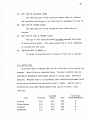
3.3 Ground Temperature
Atmospheric Environment Service (A.E.S.) has been measuring the ground
( soi 1) temperatures for many 1ocat ions across Canada.
Of the 1ocati ons
listed in Section 3.2, only 16 measure soil temperature.
The soil
temperatures at depths of 0.5 m and 1.5 m for these locations are given
below.
For further information on soil temperatures the user is referred
to the A.E.S. publication "Soil Temperature Averages 1958-1978" by
D.W. Phillips and D. Ashton, Report No. CLI3-79.
Prince George, B.C.
Soil temperature in °C at depths of
J
F
M
A
M
J
J
1.3
4.2
1.0
3.3
0.8
2.7
1.5
2.4
6.0
3.5
10.8
6.0
13.3
8.5
1.5m
0.5 m and
A
14.1
10.3
s
0
N
D
12.2
10.6
8.6
9.7
4.6
7.7
2.4
5.7
33
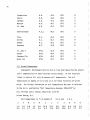
Vancouver, B.C.
J
J
15.6
12.4
17.2
14.1
J
J
13.2
10.6
17.8
14.2
21.1
17.4
A
M
J
J
F
M
A
M
5.5
8.2
6.0
7.5
7.1
7.7
9.5
8.7
12.6
10.4
s
0
17.7
15.1
16.4
15.3
A
N
D
13.6
14.3
10.1
12.2
7.2
9.9
s
0
N
D
19.3
19.7
14.1
17.4
8.4
13.7
4.0
10.0
A
Summerland, B.C.
J
F
M
A
2.1
7.1
1.6
5.5
3.5
5.2
8.2
7.3
M
22.6
19.8
Resolute, N.W. T.
F
J
M
s
A
J
N
0
D
-16.9 -19.0 -20.0 -19.7 -17.0 - 9.0 -0.2 0.7 -1.7 -6.6 -10.7 -14.3
-14.8 -16.9 -18.1 -18.4 -16.9 -12.3 -5.5 -3.0 -3.1 -5.9 - 9.2 -12.4
Swift Current, Sask.
J
-0.6
2.0
I .
M
A
M
-0.6
0.8
1.1
0.9
A
F
-1.2
1.1
s
0
N
D
12.7
11.4
8.2
9.1
3.8
6.5
0.9
3.8
s
0
N
D
16.8
12.7
13.3
12.2
7.8
9.9
2.4
6.8
-1.6
4.0
A
s
0
A
J
J
6.3
2.9
11.8
7.0
14.8
10.1
M
J
J
14.1
8.4
16.9
11.5
J
J
11.2
5.4
15.4
9.5
15.4
11.6
Saskatoon, Sask.
I
-3.8
2.1
M
F
J
-4.0
1.1
8.7
4.1
-2.0
0.6
2.2
1.0
M
A
M
-1.5
0.9
-0.1
0.8
4.5
1.8
A
Winnipeg, Man.
F
J
-1.4
2.9
-2.4
1.6
14.1 9.5
12.5 10.9
16.2
12.1
N
D
4.6
8.1
0.9
5.1
Kapuskasing, Ont.
J
F
M
A
M
J
J
0.9
3.8
0.5
3.1
0.3
2.6
0.7
2.4
5.6
3.4
12.2
7.2
15.6
10.5
A
15.8
12.2
s
0
N
D
12.7
12.0
7.9
9.9
3.6
7.3
1.6
5.1
34
Toronto, Ont.
s
J
F
M
A
M
J
J
1.3
6.6
0.4
5.4
0.9
4.5
3.6
4.9
9.3
8.1
14.5
11.8
17.5
14.6
18.7
16.5
16.3
16.3
J
J
A
s
A
0
N
0
11.1 7.5
14.3 11.9
3.6
9.2
N
D
6.4
9.9
2.9
6.9
Ottawa, Ont.
J
F
M
A
1.6
5.0
1.1
4.1
1.0
3.5
3.3
3.5
10.2
6.6
15.4
10.1
18.3
13.1
18.4
14.6
A
M
0
16.1 11.3
14.6 12.8
Val D'Or, Que.
J
F
M
A
M
J
J
0.4
2.8
0.1
2.2
0.0
1.6
0.6
1.3
6.9
3.3
13.2
8.1
16.4
11.6
16.3
13.2
s
0
N
D
13.0
12.4
7.9
9.5
3.6
6.5
1.4
4.0
Fredericton, N.B.
J
F
M
A
M
J
J
0.8
4.4
0.0
3.3
0.3
2.8
1.6
2.6
8.5
5.1
14.2
9.1
17.6
12.1
A
M
J
J
1.4
2.4
5.5
4.1
11.0
7.6
14.7
10.9
s
0
N
D
18.0
13.7
15.7
13.8
11.1
12.0
5.6
8.7
2.2
6.0
A
s
0
N
D
15.7
12.8
14.1
12.8
11.1
11.5
7.2
9.1
3.8
6.4
A
s
0
N
D
A
Charlottetown, P.E.I.
F
J
1.9
4.4
M
1.1 0.9
3.3 2.7
Truro, N.S.
J
F
M
A
M
J
J
1.9
4.4
1.1
3.3
0.9
2.7
1.4
2.4
5.5
4.1
11.0
7.6
14.7
10.9
15.7
12.8
14.1
12.8
11.1
9.1
7.2
9.1
3.8
6.4
A
s
0
N
D
12.9
11.7
10.1
10.3
6.9
8.2
4.1
6.1
St. John's, Nfld.
J
F
~~
A
M
J
J
2.2
4.2
1.4
3.2
1.2
2.7
1.7
2.5
4.9
3.9
9.2
6.8
12.8
9.7
14.1
11.6
Goose, Nfld.
J
-0.3
1.8
F
M
A
M
J
J
-1.6
0.1
-1.3
0.8
-0.7
0.8
1.5
0.6
7.6
4.5
14.0
9.4
A
14.5
11.7
s
0
N
D
11.4
11.2
6.1
8.2
2.3
5.0
-0.2
2.8
35
3.4 Modification of Collector Test Data
The performance of a solar collector is dependent on the flow rate.
If the collector flow rate for the proposed system is different from that used
when the collector was tested the FRTa and FRUL terms must be modified.
FRTa(adjusted)= r
FRTa(test)
FRUL(adjusted)= r
FRUL(test)
.
.
where r = m Cp (1 - exp[-AF'UL/(m Cp)]
(m Cp)T(1- exp[-AF'UL/(m Cp)T]
.
.
F'UL = (m Cp)T in [1- FRUL(test) A/(m Cp)T]
A
3.5 Calculation of Pipe Heat Loss Coefficient
The thermal conductance of pipe insulation is given by:
U
=
2rr k L
in
(d + 2t)
d
where d is the outside pipe diameter (mm)
t is the thickness of the insulation (mm)
L is the length of pipe (m)
k is the thermal conductivity of the insulation in W/m°C
kfibreglass ~ 0.0346 W/moc
kpolyurethane ~ 0.0245 W/moc
36
4.
DESCRIPTION OF
PROGRA~1
OUTPUT
4.1 Thermal Analysis Results
The thermal analysis of the system is printed in monthly intervals
with a yearly summary printed at the end. The results are an estimate of the
system performance of a properly designed and installed system.
The program
cannot account for improperly insulated piping, pump failure or other system
faults.
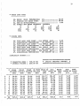
The output values are:
SOLAR INCIDENT (GJ)
Total solar radiation incident on the collector over the time period.
SOLAR COLLECT (GJ)
Solar energy transferred from the collector to the storage.
SOLAR DELIVERED (GJ)
Solar energy delivered to the space heating and hot water loads (not
including heat pump contribution).
HT PUMP DELIVER (GJ)
Energy delivered by the heat pump to the space heating load.
SPACE HT LOAD (GJ)
Space heating load (i.e. auxiliary energy that would have to be supplied
to meet the space heating load if there were no solar heating system).
AUX. SPACE HT (GJ)
Auxiliary energy required to meet the space heating load not met
by the solar heating system.
WATER LOAD (GJ)
Energy required to meet the water heating load.
37
AUX. viATER HT (GJ)
Auxiliary energy required to meet the water heating load.
The solar
contribution to the water load is the difference between this value and
the WATER LOAD.
PUMP POWER (GJ)
Total energy consumed by all pumps and fans in the system including
the heat pump.
The "TOTAL ENERGY INPUT TO ELECTRIC RESISTANCE REFERENCE SYSTEM" is
the total energy demand of a non-solar building.
If a fuel other than electricity
is used, this value should be divided by the seasonal furnace efficiency to
determine the amount of fuel required.
The "ENERGY SAVING" is the reduction in
energy achieved by adding the solar heating system (i.e. percent solar).
The "SEASONAL PERFORMANCE FACTOR" is another measure of energy savings.
This
factor. is the number of times the non-solar building auxiliary energy consumption
exceeds the solar building auxiliary energy consumption. The "MAX. HOURLY ENERGY
INPUT (MJ)" is the maximum hourly energy input of the solar building. This
value is useful for furnace sizing.
4.2
Economic Analysis
At the conclusion of the simulation year, the economic analysis is
calculated and printed.
The results of the economic analysis are extremely
sensitive to the fuel excalation rate selected.
The first value of "PRESENT WORTH" is the total cost of installing and
maintaining the solar heating system plus the cost of auxiliary energy over the
system life at present prices. The second value is the cost of installing and
maintaining the solar heating system over the system life at present prices.
38
The "LIFE-CYCLE UNIT COST" is the average price paid for building heating over
the system life in present prices (includes solar heating system).
That is,
the first value of present worth divided by the total energy load of the building
over the system life. The "SOLAR LUC" is the average price paid for the solar
energy contribution over the system life in present dollars.
39
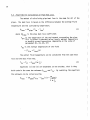
5.
PROGRAM ALGORITHM
This section describes the thermodynamic models and equations used
to simulate the solar heating system.
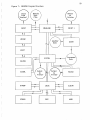
5.1 Overview of Program Operation
The basic assumption in the program is that for the purpose of thermal performance predictio n, all variables , including solar radiation , ambient
temperature and system energy flows can be considered constant for each hour.
The calculati on flow chart is shown in Figure 6.
The first step
in the program is the input from a data file of the default values of the
input parameters. The user is then able to modify the input parameters as
necessary.
After all the input parameters are set, the user initiates the
simulation (by typing "R").
If processed weather data is not available ,
the solar radiation on the tilted surface is calculate d from the horizontal
solar radiation contained in the weather data file. See Section 5.2 for a
detailed description of the algorithm.
When the processing of the weather data is completed, the program
begins the simulation. A new value of solar radiation and ambient temperature
is read for each hour simulated. Based on the new values of ambient temperature,
the space heating load and the water heating load (if necessary), are calculate d.
The space heating load is:
QHT
= UAb (Tbg - Ta) - IG
The next step is the calculatio n of the inlet fluid temperature to the
collector . This temperature is equal to the temperature at the bottom.of the
storage tank minus the temperature drop due to pipe heat loss between the storage
and collector inlet.
See Section 5.3 for a detailed description of the algorithm
for calculatio n of pipe heat loss.
Knowing the collector fluid inlet temperature
40
Figure 6:
ENERPUB Flow Chart
Start
t
[Read Default
Data
I
1
Modify Input
Data
Convert Data to
Appropriate Units
t
~5 solar radiation
on a tilted
~urface available ?
N
Calculate solar
radiation on a
tilted surface '
'
I
y
Initializ e
Parameters
2
I
t
Keaa sotar
radiation ambient
temperature
I
Calculate space
and DHW loads
•
I
t
I
Calculate
collector supply
pipe heat loss
+
L.atcutate
collector inlet
temperature
Ca ICU late
collector
performance
+
Is collector
heat gain
positive?
N,..J.,
y
Calculate
collector return
pipe heat loss
,!.,
41
T
/
-
Co 11 ector does
not operate
Calculate
building supply
pipe heat loss
t
Calculate heat
delivered to DHW
1
Calculate water
inlet temperature
to building
T
Calculate max.
possible solar
heat to load
(Osolarl
~
"'"
~obe"'Yload?
delivered!
,
y
'
Calculate
building return
pipe heat loss
1
y
Ca 1cul a.te fracCan solar heat
tion of hour thatl---- meet the full
system operates
load?
f
N
I Calculate load
!
I
not met by
solar (Qns)
I
X
l
N
Osolar
=0
42
t
N
Does the system
have a heat
pump?
y
y
Is the heat
source ambient
air?
source - Ta
T
Nt
Calculate heat
delivered by heat
pump for f~ 11
hour (0 1 J
Tsource -- Tst
f
+
Calculate heat
delivered by heat
pump for fu 11
hour (Qho)
,.
~IPartion heat load/
between solar I
and heat pump
If Qhp > Qns
Qhp = Qns
f
y
Is Qhp
>
'1'
Qht 7
Auxiliary heat
= Qns - Qhp
N
I'
!
hp = 0
Qaux = Qns
Q
y
I'
Nt
Q
I
- 0
solar Qaux = Qht - Qhp
Calculate heat
loss from load
return pipe
i
I
I
I'
II
I
I
1
43
Calculate inlet
temperature to
tank
t
Calculate new
storage
temperature
•
Sum heat flows
~
Has all the
weather data
been used?
N
Go to 2
y ' system
Output
performance
~
Calculate
Economics
t
Type S to stop
y
~
Stop
N
Go to 1
44
and the weather conditions, the collector performance can be determined.
See
Section 5.4 for a detailed description of the algorithm for collector performance.
If the collector operates for the hour, the heat loss from the collector return
piping and the fluid inlet temperature to the tank are calculated.
The next step is determination of the solar heat delivered to the load.
The temperature of the supply water to the building can be calculated knowing
the temperature of the top of the storage tank and the temperature drop due to
pipe heat loss.
The solar heat delivered to the water load is calculated by:
OsoHW = E
(Tsl - Tmains)
• QDHW
(Thot - Tmains)
where
£
is the effectiveness of the heat exchanger
Tsl is the temperature of the top of the storage tank
Tmains is the temperature of the citymains water
Thot is the hot water set point temperature
If the solar heat can supply more heat than the building needs, the
fraction of the hour that the system must operate to meet the demand is calculated.
If the solar heating system cannot meet the demand, the heat pump
is used (if available).
The energy output from the heat pump is calculated
assuming that it operates for the full hour.
of the heat pump algorithm.
See Section 5.5 for a description
If this value is greater than the heat load, then
the solar energy and heat pump energy are partioned so that they operate for the
full hour and exactly meet the demand.
If the heat pump and solar heating system
cannot meet the demand, auxiliary energy is assumed to make up the difference.
If the solar heating system supplied heat to the building, the heat
loss from the return piping is calculated. The temperature of the load return
water can be calculated knowing the pipe heat loss and heat delivered to the load.
45
At the conclusion of the hour, the new temperature(s) of the storage
tank are calculated based on the collector and load flow rates.
Section 5.6
contains a detailed description of the stratified storage tank algorithm.
Finally, the hourly heat flows are summed for the simulation period
and the monthly and yearly totals displayed on the printer.
analysis is performed at this point.
of the economic analysis algorithm.
The economic
See Section 5.7 for a detailed description
46
5.2 Algorithm to Process Weather Data
Most Canadian weather stations measure only total solar radiation on
a horizontal surface.
Most solar collectors, however, are tilted toward
the sun to increase the incident solar radiation.
The program determines
hourly values of total solar radiation (beam, diffuse and reflected) on
a tilted surface and stores ' the values in a scratch file.
The algorithm
for converting horizontal solar radiation to tilted solar radiation is
similar to the method used in Duffie and Beckman (1).
In order to estimate the solar radiation on a tilted surface it is
necessary to split the total measured horizontal solar radiation into its
two components:
It is possible to estimate the amount
beam and diffuse.
of diffuse solar radiation from the ratio of the measured solar radiation
to the extraterres trial solar radiation.
If this ratio is low then the
solar radiation must be mostly diffuse; if this ratio is high the solar
radiation must be mostly beam.
When the beam and diffuse solar radiation components are known, standard
geometric relations can be used to estimate the solar radiation components
on a tilted surface.
When estimating solar radiation on a tilted surface
a third component is introduced:
reflected radiation.
Reflected radiation
can be estimated from the beam radiation and the ground albedo or
reflectivity .
The program equations and execution procedure are given below.
At the start of each day the solar constant and the earth's solar
declination are calculated.
sc
= 4871.D
The solar constant is given by
(1. + 0.33 cos
(2~N
I 365))
where N is the day' number (Jan 1 is 1).
in KJ/(hr'm 2 )
47
The earth's declination is given by
o = 23.45 *
360
2~
*sin (
(in radians)
(284 + N))
360 *365
2~
These values are assumed constant for each day.
All other calcu-
lations are made on an hourly basis.
The first step is to read the measured weather values from the data
For each hour the weather data file contains six values in the
file.
following order.
1)
2)
3)
4)
5)
6)
month number (1-12)
day number (1-31)
hour number (1-24)
ground reflectivity
solar radiation on a horizontal surface (in Watts/m2 )
ambient temperature (in °C)
The extraterrestrial solar radiation on a horizontal surface is
calculated by
cos (az)
Hex = Sc
where cos (az) is cosine of the zenith angle (angle between the beam and
the vertical)
cos (az) =cos
~
(~)
cos (o) cos w +sin~ sino
is the latitude of the location
w is the hour angle.
The diffuse solar radiation (Hd) can be estimated using a correlation
by Orgill and Hollands (2).
Hd = 0.1769·H
if
o. 75
<
KT
Hd = (1.55699- 1.84013 ' KT)'H
Hd = (1. - 0.248857 ' KT)'H
~
if 0.35
if 0.0
~
where H is the measured hourly solar radiation
KT
~
KT
0.35
~
0.75
48
KT is the ratio of measured solar radiation to the extraterrestrial
solar radiation
= H I Hex
The beam radiation (Hb) is simply the total measured solar radiation
minus the diffuse radiation.
The next step is to calculate the ratio of beam radiation on the
tilted surface to that on the horizontal surface (Rb).
Rb
= cos (eT)
where cos
1 cos (ez)
(eT) is the cosine of the angle of incidence of beam radiation,
between the beam and the normal to the surface.
cos (eT)
= sin (a) sin
(<I>) cos (s)
- cos (a) cos
(<I>) cos (s) cos (w)
cos (a) sin (cp) sin (s) cos (y) cos (w) cos (a) sin (s)
sin ( y) sin (w)
y is the azimuth angle measured from south (east is positive, west is
negative)
Thus, the beam solar radiation on the tilted surface is
The diffuse solar radiation component on the tilted surface is estimated
using the radiation view factor from the collector to the sky with correction
factors for non-uniform distribution of diffuse radiation.
The correction factors for anisotropic diffuse radiation are taken from
and Klucher ( 4 ). The resulting equation is
Temps and Coulson ( 3
H = (1 + cos (s)) (1 + F sin 3 (sl2)) (1 + F cos 2 (eT) •
dT
2
sin 3 (ez)) Hd
where ·F = 1 - (HdiH) 2
+
I
I
49
The reflected solar radiation on the tilted surface (Hr) is
H = (1 - cos (s)) P H
2
r
Where
p
is the ground reflectivity
The total solar radiation on the tilted surface (HT) is the sum
of the beam diffuse and reflected solar radiation components.
Hourly values of total solar radiation on a tilted surface, ambient
temperature, day number and hour number are written to the scratch file.
When all the data has been processed and written to the scratch file,
the file is rewound to be ready for the system simulation.
so
5.3 Algorithm for Calculation of Pipe Heat Loss
The method of calculating pipe heat loss is the same fOr all of the
pipes.
The heat loss is based on the difference between the average fluid
temperature and the surrounding temperature.
Qloss
= UApipe
( 1)
(Tfm - Tenv)
where UApipe is the pipe heat loss coefficient
Tenv is the temperature of the environment surrounding the pipe.
This is either a constant value, hourly ambient temperature
or monthly ground temperature (depending on the value of
parameters 61, 63, 65, 67)
Tfm is the average temperature of the fluid
= (Tfin
+ Tfout)/ 2
The outlet fluid temperature can be calculated from the pipe heat
loss and the mass flow rate.
Tfo
.
(2)
= Tfi - Qloss/(m CP)
Equations (1) and (2) are dependent on one another, that is they
both contain the same two unknowns Qloss and Tfo'
the unknowns can be solved exactly.
Qloss
= UApipe(Tfin - Tenv)/( 1 + UA~ipe)
2 m cp
By combining the equations
51
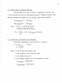
5.4 Algorithm for Solar Collector Performance
The instantaneous performance of solar collectors is represented by
the standard Hottel-Whillier-Bliss model of FRTa and FRUL. The program
assumes that both these collector characteristics are independent of
temperature and solar radiation.
If a collector-to-storage heat exchanger is used, the FRTa and
FRUL are modified according to the method of DeWinter ( 5 ).
where Ex
.
.
= mcCp I (m Cp
and the
+ FRUL * (1 - Ehx)l Ehx)
on a value means that it includes the effect of the heat
1
exchanger.
For each hour, the reduction in solar transmission of the collector for
non-normal angles of incidence is calculated. This reduction (K) is given
by:
where b0 is the incident angle modifier
a is the incident angle of the beam radiation on the collector
To determine if the collector will operate for a given hour, the
stagnation temperature (Tc) is calculated.
Tc
= Ta
+
HT. K. FRTa 1 I FRUL 1
If Tc is greater than the inlet temperature, the collector is assumed
to operate for the full hour.
If Tc is less than the inlet temperature the
collector does not operate. The heat collected by the collector is
Qc = FRUL1
•
Area • (Tc - TCl. )
The collector outlet temperature is
Teo
= Tci
.
+ Qc I (mcCp)
52
5.5 Algorithm for Heat Pump
The energy delivered by the heat pump (Qhp) is estimated by using a
correlation between energy output and the source or heat pump evaporator
temperature (Te).
The energy consumed by the heat pump (Php) is estimated
in a similar manner.
2
Qhp = alTe + a2Te + a3
2
Php +biTe + b2Te + b3
where a1, a2, a3 and b1 , b2, b3 are correlation coefficients
The correlation coefficients can be estimated from the heat pump
performance curve, available from the heat pump manufacturer.
Alternatively,
performance data points can be entered into the program and the program
will generate the coefficients using a least squares analysis.
The heat pump operation is assumed to be steady state for each one·hour time step of the simulation. This implies that the temperature of the
heat source, whether the solar storage tank or ambient air, is constant
over the hour or the fraction of the hour needed to meet the load.
The coefficient of performance (COP) of the heat pump is defined as:
A heat pump can only operate within specific ranges of temperatures.
If the evaporator temperature is outside this range, the internal control system j
will
prevent the heat pump from operating.
To simulate this operation,
the program checks at the beginning of the hour to see if the source temperature is between the minimum and maximum values.
If it is outside of
this range, it is assumed that the heat pump does not supply any heat for
that hour.
53
5.6 Algorithm for Stratified Storage Tank
Water storage tanks in solar systems will exhibit some temperature
stratification. The magnitude of the stratification depends on system
flow rates and temperatures.
mended by Klein ( 6 ).
The model used in the program is as recom-
This model is similar to, yet more flexible than,
the model given in Duffie and Beckman ( 1).
The tank is modelled as a series of horizontal nodes.
A mass and
energy balance is performed on the nodes for each simulated hour.
The
water entering the tank (from either the load or the collector) is assumed
to rise or fall to the node closest in temperature.
If water is flowing
from the load and the collector, the fluid streams are assumed fully mixed
before they enter each segment.
The energy balance on the tank also takes
into account the heat lost by each node to the environment and the heat
transferred from the storage top node to the domestic hot water by means
of the DHW heat exchanger.
A heat balance on a storage node gives:
.
.
T51.' = T51. +[a.1 mc Cp (Teo- Tsi) + Si mLCp (Tlo- Tsi)-
where T5 i is the temperature of the node i at the beginning of the hour
T5 i' is the temperature of the node i at the end of the hour
me' mL are the hourly mass flows from the collector and load to the
storage
CP is the specific heat of water
mi
is the mass of the water in node i
01055 is the amount of heat lost to the environment by conduction
out the storage walls
Qup' Qdown is ~he amount o~ heat transferred into the node by flow
com1ng up or go1ng down
54
a, 6 are control functions that define the node(s) where the
fluid effectively returns
The control functions are given by:
then ai = 1 I
(I rc
- ScI + 1)
otherwise ai = 0
then 6. = 1/(lrL1
\I
+ 1)
otherwise 6·1 = 0
where rc is the node number where the collector fluid returns
rL is the node number where the load fluid returns
sc is the node number to which the collector return fluid is closest
in temperature
\
is the node number to which the load return fluid is closest
in temperature
The quantity Qdown is given by :
for
Yj > 0
(Ts.1- 1 - Ts.)
1
N
i-1
.
where yi = mccp E Clj
mLCp E
j=i
j=1
'down --
0
Yi
-
otherwise Qdown = 0
The quantity Qup is given by
for yi+ 1
<
0
6j
55
After the temperatures have been updated, two checks are made in the
program.
The first check is for storage temperature instability.
If the
temperature of a node is greater than the one above it, it is assumed that
density differences will cause perfect mixing of these nodes.
Because all the
nodes have equal thermal capacity, the new temperature of the nodes is the arithmatic average of the mixing nodes.
temperature.
The second check is on the minimum allowable
If the temperature of any of the nodes goes below the minimum
allowable temperature, it is assumed that an auxiliary heater comes on.
Because
the heater is most probably placed in the bottom of the tank, the heated water
will rise and cause a fully mixed tank.
warning flag is printed.
If the heater has to come on a
56
5.7 Algorithm for Economic Analysis
The algorithm for economic analysis is standard and is given in many
economic textbooks.
Two economic indicators are calculated: (i) present
worth of solar savings (with and without auxiliary energy) (ii) lifecycle unit cost of energy (with and without solar heating system).
In the present worth analysis, all future payments, whether for fuel
or bank loans, are discounted back to present. The present worth of yearly
expenditures for fuel and maintenance are:
N
P.W.f = E C
(1 + i)N 1 (1 + r)N
i= 1 fuel
N
P.W.m = E C
I (1 + r)N
i= 1 main
where Cfuel, Cmain are the.first year costs for fuel and maintenance
respect1vely
i is the fuel inflation rate
r is rate of return on the best alternative investment
The present worth of the loan repayments is
P.W.ss = C 1 (1 + l)L ((1 + r)L- 1.)
ss ((1 + l)L - 1.) r(1 + r)L
where Css is the total cost of the solar system
1 is the interest on the loan
L is the loan period in years
The salvage value is discounted back to present by:
P.W.sal = csall (1 + r)N
Thus, the present worths of the solar investment with and without
fuel costs are:
P.W.solar
1
= P.W.ss
+ P.W.m - P.W.sal
57
P.W.solar
2
= P.W.ss
+ P.W.m + P.W.f - P.W.sal
These are the values printed in the economic analysis.
cycle unit costs can be found from the present worth.
The life-
The life-cycle
unit cost is
LUC
= P.W.solar I Etot
1
where Etot is the total heating load over the system life
The solar life-cycle unit cost is
SLUC
= P.W.solar I (Etot • Fs)
2
where Fs is the fraction of the heating load met by the solar heating system
58
6.
PROGRAM STRUCTURE
The purpose of this section is to describe the program structure.
Only those individuals interested in modifying the program need read this
section.
The program flow chart is shown in Figure 7. The program consists
of a mainline and 16 subroutines:
i)
MAINLINE- main program for file unit number allocation and calling of
subroutines.
ii)
PRINT 1 - subroutine to print title page at start of program.
iii)
PRINT 2 - subroutine to print hourly energy analysis summaries.
iv)
INPUT - interactive subroutine for user input of data and printing of
input data. This subroutine reads the default data from a data
file.
v)
WEATH - subroutine for converting measured horizontal solar radiation to
the tilted surface. The weather data is read from a data file
and the processed data is written to a new file.
vi)
SYSTEM- subroutine to initialize system parameters and sum the system energy
flows. At the conclusion of the simulation the yearly results
are printed.
vii)
LOGIC- subroutine to call the component subroutines depending on energy
flows.
viii)
LOAD - subroutine to calculate water and building heat loads and the solar
contribution to these loads.
ix)
x)
CLECTR - subroutine to calculate collector performance.
HTPUMP - subroutine to calculate heat pump performance.
xi)
PIPE - subroutine to calculate heat loss from a pipe (used for all four
pipes).
xii)
STORG3 - subroutine to calculate the new temperature(s) of the storage
tank at the end of the hour.
xiii)
xiv)
xv)
ECONAL - subroutine to perform economic analysis.
TGRD - subroutine to determine monthly ground temperature.
HPCOEF - subroutine to determine heat pump power input and output characteristics
59
Figure 7:
ENERPUB Program Structure
Input
from
Terminal
Output
to
Printer
Default
Data
File
T
1
INPUT
PRINT 1
MAINLINE
II
tr
HPCOEF
-1 I
Weather 1-Data
rl
WEATH
-
LEAST
n
Processed
Data
SYSTEM
CALF UN
II
ECONAL
1--
HTPUMP
Ir
STORG3
Output
to
Printer
Output
to
Printer
LOGIC
TI.
I
\--
PRINT2
CLECTR
II
i
PIPE
!
I
LOAD
I
60
xvi)
xvii)
CALFUN- subroutine that contains general form of heat pump power
equation.
LEAST- subroutine to perform least squares analysis on heat pump
power data points.
Four file definitions must be made before the program can be run:
Terminal/Printer - (Unit 12) is the device for data input and program
output
Default Data - (Unit 10) is the file that contains default data for the
system parameters.
Weather Data - (Unit 8) is the file that contains the TRNSYS compatible
weather data. The data must be written in the format
(2X,I2,2X,I2,2X,I2,F3.1,I3,F6.1) and contain month
number, day number, hour number, ground reflectivity,
ambient temperature (°C) and solar radiation on a horizontal
surface (W/m 2 ).
Processed Data - (Unit 9) is the file that is created by the program
containing the solar radiation on the tilted surface,
and the ambient temperature.
61
7.
REFERENCES
1)
Duffie and Beckman, Solar Engineering of Thermal Processes, John Wiley
and Sons, New York, 1
2)
Orgill, J.F. and Hollands, K.G.T., Solar Energy, Vol. 19, No.2, "Correlation
Equation for Hourly Diffuse Radiation on a Horizontal Surface".
3)
Temps, R.C. and Coulson, K.L., Solar Energy, Vol. 19, No. 2, "Solar
Radiation Incident upon Slopes of D1fferent Orientation".
4)
Klucher, T.M., Solar Energy, Vol. 23, No. 2, "Evaluation of Models to
Predict Insulat10n on Tilted Surfaces".
5)
de~Jinter,
6)
Klein, S.A., A Design Procedure for Solar Heating Systems, Ph.D. Thesis,
University of W1sconsin-Mad1son, 1976.
F., Solar Energy, Vol. 17, "Heat Exchanger Penalties in DoubleLoop Solar Water Heat1ng Systems".
62
8.
INPUT DATA WORKSHEET
ENERPUB Commands
L - TO
I - TO
C - TO
S - TO
TO CHANGE
OBTAIN DATA LISTING
105 PROGIA! (VITH LISTIIG)
CHANGE SY5TEM TYPE
STOP SESSION, OR •••
PAIA!ETEI, TYPE CODE HD!BER
ENERPUB Input Data With Default Values
*
GENERAL SYSTEM DATA
1.
2.
3.
4.
5.
6.
7.
*
SIMULATION B~GINS IN Y~Ad •••••••••••••••••• 1970
365
SIMULATION PERIOD (DAYS)•••••••••••••••••••
DAY1 OF THE PERIOD (1-365) •••••••••••••••••
1
DETAILED PRINT-OUT (NO=O,YES=I-HR INTERVAL)
0
STARTING HOUR OF PRINT INTERVAL (O, •• ,I) •••
0
TILTED ANGLE OF COLLECTOH. (U~GREES) •••••••• 55.00
COLLECTOR ORIE~TATION (SOUTH=O.,~EGREES) •••
o.oo
COLLECTOR DATA
10.
11.
12.
13.
14.
15.
COLLECTOR AREA tM2) •••••••••••••••••••••••• 100.UO
MAXIMUM OUTLET TEMP. (C)••••••••••••••••••••
98.
DIFFEHENTIAL TEMPEHATURE (C)...............
1.70
PUMP POWER/ COLLECTOR AREA (W/M2)•••••••••
0.
FLOW RATE* HT.CAPACITY (W/M2-C)...........
60.
FB-TAU-ALPHA••••••••••••••••••••••• •••••••• 0.710
16. FR-UL
(W/M2-C)••••••••••••••••••••••••••••
3.91
17. 80, CO~FF. FOR INCIDENT ANGLE MODIFlER ••••• -0.100
18. COLLECTOR-STORAGE HX EFF~CTlVENESS ••••••••• 1.000
*
STORAGE DATA
20.
21.
22.
23.
24.
25.
26.
27.
28.
29.
STORAGE VOLUME/COLL.AREA
(M3/M2) •••••••••• 0.075
STARTING TEMPERATURE (C) ••••••••••••••••••• 20.00
SURROUNDING TEMPERATURE (C)•••••••••••••••• 20.0
TOP HEAT LOSS COEFF. (W/C)••••••••••••••••• o.oo
SIDE HEAf LOSS COEFF. (W/L)•••••••••••••••• 0.00
BOTTOM HEAT LOSS COE~F- (W/Cl•••••••••••••• 0.00
t OF STRAT~FICATION TANK SEGMENTS ••••••••••
1
SEG. i FOR COLLECTOR RETURN INfO TANK ••••••
1
SEG. i FOR BUILDING RETURN INTO TANK •••••••
1
~.ou
M~NI~UM ALLOWABLE STORAGE TEMP. (C)•••••••••
63
*
HEAT PUMP DATA
30. LOWER Ll~Ir OF EVAPORATOR TEMP. (C) •••••••••
31. HIGHER LIMIT Oi' EV!lPORATOil Tl>Mt'. (C)........
32. COEFF~ClENTS CQ, CP OF HEAT PU~P :
*
BUILDING DATA
40.
41.
'12.
43.
44.
45.
46.
*
BUILJJING UA COEFF. (W/C) ••••••••••••••••••• 1000.0 - - - - - - 0.
POWEll FOR HJ:;AIING FAN (~)••••••••••••••••••
STOR.i!GE-IJUILDING iiX EH'ECTl.VJ::NESS •••• •••••• 0. 700 ------------MIN.CaPACirANCE ilAI£ Of LOAlJ H.:. (W/C) •••••• 3000.
0.00 -----------DIRECT SOLAR GAIN i'ACTOR (M2) ••••• •••••••••
INDOOR DESIGN iE~PEliATURE (C) •••••••••••••• 20.00---------INTERNAL HOURLY HEAT GAIN SCHEDULE (KJ)
1800.
o.
o.
o.
o.
o.
3600.
1800.
4500.
5400.
2700.
3600.
16200.
1800.
2700.
2700.
J6UO.
4500.
1800.
1800.
2700.
2700.
2700.
6300.
WATER LOAD DATA
so.
6.00
40.00
51.
52.
53.
*
0.0 ------------35.0 -------------
o. so
o.
o.
o.
o.
Pl.PING DATA
60.
61.
62.
63.
64.
65.
66.
67.
PIPE HEAT LOSS COEFF - COL RETURN (W/C) •• ••
SURROUNDING TE~P~RATURE- COL RETURN (C) •••
PIPE HEAT LOSS COEFF- COL SUPPL¥ (W/C)....
SURROUNDING TEMPERATURE- COL SUPPLY (C) •••
PIPE HEAT LOSS COEFF - BJJG SUPJ?LY (W/C)....
SURROUNDING TEMPERATURE- BOG SUPPL¥ (C) •••
P~PE HEAT LOSS COEi'F - BOG RETURN (li/C).. ••
SURROUNDING TEaPERATURE- llDG RETURN lC) •••
u. 00
20.0
0.00
20.0
0.00
20.0
0. 00
20.0
64
*
EC01WMIC DATA
70. SYSTEM LIFE (YEARS)••••••••••••••••••••••••
20------------
71.
TERM OF· LOAN
INI~REST RAT~
20 - - - - - - - - - - - -
72.
73.
74.
75.
76.
77.
78.
79.
dO.
81.
82.
(YEARS) •••••••••••••• •••••••••
OF LOAN •••••••••••••••••••••• O.luO -----------RATE OF RETURN (DISCOUNT HATE) •••••••••••• ·• 0.1UU -----------FIXED COST OF SOl..Ail COi'IPONi::NiS ($) •••••••••
83U.
FIAED COST OF HEAT PUMP ($)•••••••••••••••• 2180.
Y~AHLY ftAINTENANCE COST OF SOLAR COMP.($/Y)
50.
IEARLI ft&INIENANCE COST OM HP. {S/IR)......
SO.
SALVAGE VALU~ AT END 0£ PERIOD ($).........
0.
UNIT COST OF COLLECTUH ($/M2) ••••••••••••••
230.
UNIT COST OF STOHAGE ($/M3)................
122.
UNIT COS£ Oi FUEL AT PRESENT (S/GJ) •••••••• 10.000 ----------INFLATION RATE OF ENEBGI :
0.130
0.130
0.130
0.130
0.130
0.100
0.100
0.100
0.100
0.100
0.100
0.100
0.100
0.100
0.100
0.100
0.100.
0.100
u.lOO
0.100
65
9.
NOMENCLATURE
a
heat pump coefficients
A
collector area (m2 )
b
heat pump coefficients
bo
incident angle modifier
cfuel
first year fuel cost ($/yr)
cmain
COP
first year maintenance cost ($/yr)
cP
specific heat (KJ/{kg"°C)
csal
salvage value ($)
css
DHW
total cost of the solar system ($)
domestic hot water load (litres)
Etot
total heating load over system life (GJ)
Ex
heat exchanger factor
FR
collector heat removal factor
FR'a
collector transmission-absorption coefficient
FRUL
collector heat loss coefficient (W/(m 2 "°C)
Fs
fraction solar
H
measured hourly solar radiation (KJ/(hr"m 2 )
Hb
beam hourly solar radiation
HbT
beam hourly solar radiation on a tilted surface (KJ/(hr"m 2 )
Hd
diffuse hourly solar radiation
HdT
diffuse hourly solar radiation on a tilted surface (KJ/(hr"m 2 )
Hex
extraterrestrial hourly solar radiation
HP
heat pump
Hr
reflected hourly solar radiation (KJ/(hr"m 2 )
coefficient of performance
(KJ/(hr"m 2 )
(KJ/(hr"m2 }
(KJ/(hr"m 2 )
66
HX
heat exchanger
i
fuel inflation rate
IG
internal heat gain (KJ)
KT
clearness index
1
loan interest rate
L
loan period (years)
LUG
life-cycle unit cost
m
mass flow rate (kg/hr)
me
mass flow rate through the collector (kg/hr)
mi
.
ml
mass of water in node i (kg)
N
day number of the year
P
pump
Php
heat pump energy input (KJ/hr)
P.W.f
present worth of fuel expenditures ($)
P.W.m
present worth of maintenance expenditures ($)
P.W.sal
present worth of salvage value ($)
mass flow rate to the load (kg/hr)
P.W.solar present worth of solar investment ($)
P.W.ss
present worth of loan repayments ($)
Qaux
auxiliary heat requirement (KJ/hr)
Qc
solar energy collected by collector (KJ/hr)
QDHW
domestic hot water heating load heat transfer (KJ/hr)
Qdown
heat storage nodes (KJ/hr)
Qhp
heat pump energy output (KJ/hr)
QHT
space heating load (KJ/hr)
Qload
space heating load (KJ/hr)
67
Qloss
heat loss from pipe or tank (KJ/hr)
Qns
heat load not met by solar (KJ/hr)
QSDHW
solar contribution to DHW load (KJ/hr)
Qsolar
maximum possible solar contribution (KJ/hr)
Qup
heat transfer between storage nodes (KJ/hr)
r
rate of return
node number where the collector fluid returns
node number where the load fluid returns
ratio of beam radiation on tilted surface to horizontal surface
node number to which the collector return fluid is closest in temperature
node number to which the load return fluid is closest in temperature
solar life-cycle unit cost
Ta
ambient temperature (°C)
building temperature (°C)
(°C)
\
collector stagnation temperature
Tci
collector inlet temperature
Tco
collector outlet temperature
Tenv
temperature of the environment surrounding the pipe (°C)
Tfin
collector fluid inlet temperature (°C)
Tfout
collector fluid outlet temperature (°C)
Thot
hot water set point temperature (°C)
Tmains
city mains water temperature (°C)
Tsl
Tsi
temperature of the top of the storage tank (°C)
Tsource
heat pump source temperature
Tst
storage temperature
(°C)
( °C)
temperature of storage node i (°C)
( °C)
(°C)
68
building heat loss coefficient (W/°C or KJ/(hr°C)
pipe heat loss coefficient (W/°C or KJ/(hr°C)
collector heat loss coefficient (W/(m 2 °C)
Cl
solar absorptivity
y
azimuth angle
1T
3.14159
p
density ( kg/m3 )
"'i
stratified storage constant
yi
stratified storage constant
tli
stratified storage constant
e
incident angle
EBERPUB MANUAL:
ERRATA NOTICE
The following corrections apply to the ENERPUB Users Manual, November 1982:
Page 42
"Partion heat load" should read "Partition heat load"
Page 44, line 20
"partioned" should read "partitioned "
Page 46, line 25
Sc should read SC
Page 47, line 16
Sc should read SC
Page 66
the amount of heat transferred into the
storage node when flow goes down
Page 67
the amount of heat transferred into the
storage node when flow goes up
Page 67
SR4'f/A
sc
solar constant
. I