1
A Guide to Using
RISKMAN
Stochastic and Deterministic Population
Modeling RISK MANagement Decision Tool
for Harvested and Unharvested Populations
Version 1.9.003
September 30, 2006
Mitchell Taylor
Martyn Obbard
Bruce Pond
Miroslaw Kuc
Diana Abraham
RISKMAN
Version 1.9.003
User Manual
September 30, 2006
Mitchell Taylor1
Martyn Obbard2
Bruce Pond2
Miroslaw Kuc3
Diana Abraham4
1
Wildlife Division, Department of Sustainable Development,
Government of Nunavut, P.O. Box 1000, Station 1170, Iqaluit, Nunavut X0A 0H0
2
Ontario Ministry of Natural Resources, Wildlife & Natural
Heritage Science Section, 300 Water St., 3rd Floor North, Box 7000, Peterborough, ON, K9J
8M5
3
PH 205 – 942 Yonge St., Toronto, Ontario, M4W 3S8
3
ESSA Technologies Ltd.
Suite 301, 1595 16th Avenue, Richmond Hill, Ont., L4B 3N9
© The Queen’s Printer for Ontario, 2006
No part of this publication may be reproduced, stored in a retrieval system, or transmitted, in any form or by any means,
electronic, mechanical, photocopying, recording, or otherwise, without prior written permission.
Contents
System Overview
1
General Overview...................................................................................................................... 1
Hardware and Software ............................................................................................................. 2
Installation Instructions.............................................................................................................. 2
Concepts and Common Functions
3
Overview ................................................................................................................................... 3
Life Table Matrices.................................................................................................................... 3
Modifying Data in Matrices ........................................................................................ 3
Blocking Multiple Matrix Cells for Data Entry........................................................... 4
Matrix Import and Export............................................................................................ 5
Strata Definition......................................................................................................................... 6
Entering and Modifying Strata .................................................................................... 6
Strata Definition Example ........................................................................................... 9
Density Dependence ................................................................................................................ 10
Density Dependence Definition................................................................................. 10
Density Dependence Interface................................................................................... 12
Density Dependence Plot .......................................................................................... 14
Effect of Density Dependence on Litter Size ............................................................ 14
Variance................................................................................................................................... 15
Parameter and Environmental Uncertainty................................................................ 15
Co-variance ............................................................................................................... 17
The “Mean” Look at Growth Rates ......................................................................................... 17
Mean Growth Rate Definition ................................................................................... 17
Implementation in RISKMAN .................................................................................. 18
User Interface
20
Overview ................................................................................................................................. 20
File Menu................................................................................................................................. 20
Open Project .............................................................................................................. 21
Save Project and Save Project As.............................................................................. 22
Project Description .................................................................................................... 22
Exit ............................................................................................................................ 23
Parameters Menu ..................................................................................................................... 23
Recruitment ............................................................................................................... 23
Individual Survival .................................................................................................... 25
Hunting Mortality...................................................................................................... 26
Other Mortality.......................................................................................................... 34
Initial Population ....................................................................................................... 35
Output Menu............................................................................................................................ 38
Print Graphs............................................................................................................... 38
View .......................................................................................................................... 38
Spreadsheet Export.................................................................................................... 39
i
RISKMAN Export..................................................................................................... 40
Vital Rates Export ..................................................................................................... 40
Options Menu .......................................................................................................................... 41
Preferences ................................................................................................................ 41
Species Definition ..................................................................................................... 43
Setup Graphs ............................................................................................................. 46
Colours and Line Styles............................................................................................. 48
Help Menu ............................................................................................................................... 48
Running the Model .................................................................................................................. 49
Display Graphs .......................................................................................................... 51
Schedule A
52
End User Licence..................................................................................................................... 52
Literature
54
References ............................................................................................................................... 54
RISKMAN Papers ................................................................................................................... 55
Glossary of Terms
56
Index
57
ii
RISKMAN
System Overview
System Overview
General Overview
This document describes the structure and operation of RISKMAN (RISK
MANagement) - a computer simulation system intended as a decision support tool for
managers of harvested and unharvested populations who must base their decisions on
uncertain information. RISKMAN employs a Monte Carlo approach similar to that
used in population viability models to estimate the uncertainty of population
trajectories based on estimates of population numbers and demographic parameters.
RISKMAN has two distinct uses:
*
as a management tool, the system can be used by wildlife managers to design
management strategies and regulations for specific populations of wildlife; and
*
as a research tool, the system can be used to investigate the behaviour of
populations under various management regimes and to investigate and understand
the effects of uncertainty on population persistence.
Background and General Description
The development of RISKMAN is a collaborative effort, funded jointly by the
Ontario Ministry of Natural Resources (OMNR) and the Nunavut Department of
Sustainable Development. RISKMAN has its roots in a series of polar bear
workshops intended to develop quantitative tools to determine the impact of harvest
on polar bear populations, and the OMNR's interest in establishing a firm basis for
managing black bears. RISKMAN has an annual, biannual and three-year life cycle
options to allow accurate modelling of all bear species. RISKMAN is capable of
simulating the population dynamics of most harvested wildlife species.
At the core of RISKMAN is a simple life-table model (Cole 1954, Caughley 1997),
comprised mostly of "bookkeeping" functions associated with births, deaths, and
ageing of animals in the simulated population.
RISKMAN allows users to select the model that correctly describes the life history
biology of their target species (e.g., annual for furbearers and ungulates; two-year for
black bears, or three-year for polar bears, grizzly bears and elephants). The user can
define the number of age classes, and set the survival and recruitment rates for
appropriate age strata, or for each age individually. Harvest scenarios can be
1
RISKMAN
System Overview
simulated by defining the number of annual hunting seasons (none, single or two), the
quotas (or fraction of the population) of animals to be harvested, and relative
selectivity/vulnerability of age/sex classes to hunting and non-hunting (humaninduced) mortality.
RISKMAN has both a deterministic and a stochastic mode. The stochastic option is
an individual based model using the variance of input parameters to provide Monte
Carlo estimates of the uncertainty in simulation results. The rationale for the model
structure and approach to variance is provided in a companion technical paper (Taylor
and Cluff, 2002). RISKMAN also has the capability to include density effects. The
user can specify a relationship of any of the vital rates (survival, proportion with
litters, and litter size) to the density of in population sex or age strata.
Hardware and Software
RISKMAN has been developed to run in a Microsoft Windows 2000 or XP
environment on a standard PC. It does not require any additional hardware or
software beyond that associated with normal operation of Windows.
Some of the data can be exported into a “CSV” format, which is compatible with all
major spreadsheet format (e.g. Microsoft Excel).
RISKMAN's interface uses standard conventions and keystrokes for Microsoft
Windows-based software.
Installation Instructions
If you have an earlier version of RISKMAN installed on your computer, you should
remove it using the Start button “Settings / Control Panel / Add-Remove
Programs” utility.
Make sure to save any project files created with the previous version of the system.
You will be able to continue to use them with the new version.
To install RISKMAN:
1. Close any open programs.
2. Insert the RISKMAN CD into your CD drive or place the downloaded program in
a temporary directory.
3. Double-click on the “RiskmanSetup.exe” program.
Follow the prompts as the program asks you for the installation location and other
installation details.
2
RISKMAN
Concepts and Common Functions
Concepts and Common Functions
Overview
This section describes some of the concepts needed to better understand RISKMAN,
and functions and procedures that are common to many of the program’s features.
For simplicity they are described once here rather than repeatedly throughout the
manual. For specific details about each menu and screen, see the User Interface
section.
Life Table Matrices
In order to simulate population changes that result from management decisions, users
will likely be modifying or entering new data, changing age and encumbrance
(females with offspring) groupings, selecting various density dependence
relationships, and testing the effect of stochasticity on the results of simulation runs.
Most of these options can be accessed from the life table screens present in the
Parameters Menu.
Modifying Data in Matrices
For each life table screen under the Parameters Menu, the dimensions of the matrix
are determined by:
*
the parameters entered in the Species Definition screen under the Options Menu
*
by the user-defined age class and encumbrance (females with or without
offspring) categories (i.e., strata), and
*
by the Information Display Format selected in the Strata Definition screen.
Additionally, the tables for recruitment and individual survival each contain four
layers of data that can be accessed by clicking on tabs across the top of the table. The
four tabs are: Rates, Standard Error, Carrying Capacity, and Shape Factor (KS). The
Rates tabs contain base parameter data; the Standard Error tab contains measure of
variability for stochastic simulations; the Carrying Capacity and Shape Factor tabs
contain values describing the density dependent relationship.
3
RISKMAN
Concepts and Common Functions
To enter or modify values in the life table screens:
1. Select the cell to be modified by highlighting it with a click of the mouse. (Click
again if you wish to modify individual digits in the cell.)
2. Type in the new value or digit.
3. If you wish to enter the same value into two or more adjacent cells in a block, use
the blocking feature to simplify the process.
4. To save your changes to a life table matrix and return to the Main Menu screen,
click OK.
The Standard Error tab for both Recruitment and Individual Survival screens is
available only when the model is set to run in Stochastic mode on the Preferences
screen in the Options Menu. Standard error values can be modified using the system
edit features.
Estimates of demographic parameters typically pool together the parameter
uncertainty (due to sample size) and the environmental uncertainty (annual and
individual differences). The Preferences screen in the Options Menu allows the user
to partition the standard error into a parameter and environmental component. The
parameter component is modelled by obtaining a random deviate (using the parameter
portion of the total standard error) that serves as the mean for that particular run. A
Monte Carlo simulation consists of many runs. The environmental component is
modelled by using the run mean and the environmental portion of the total standard
error for random variate for each iteration (year) of a given run. The recommended
apportionment of the standard error is 75% parameter and 25% environmental
uncertainty when the actual distribution has not been estimated. For further
discussion and examples of the parameter and environmental uncertainty see the
Variance section.
The remaining two tabs, Carrying Capacity, and Shape Factor (KS), are available
only when Density Dependence is turned on (Species Definition screen in the Options
Menu). These two parameters work together to define how the number of animals
influences the behaviour of other population parameters such as the proportion of
females with litters, mean litter size, survival, etc. For further discussion on density
dependence see the Density Dependence section.
Blocking Multiple Matrix Cells for Data Entry
To select a block of cells, left-click on one of the corner cells of the block and rightclick the opposite corner. The cells of the selected block will change colour and a
pop-up menu will appear that shows the available actions.
4
RISKMAN
Concepts and Common Functions
Enter Value - inserts the number you wish to enter into each cell of the block
Clear - resets all cells in the block to 0
Exit Without Action - select this option to leave the Available Operations
screen without making any changes, or press the <Esc> key on
your PC keyboard
To re-define an already selected block, right-click on the new corner cell. To
unblock, simply left-click on any cell.
Matrix Import and Export
The Import and Export command buttons are located on the right side of all
Parameters Menu screens.
The export function converts the currently open matrix to comma and quote delimited
ASCII format and saves it in a user defined file. ASCII format is suitable for
importing into a spreadsheet or database application, or back into RISKMAN (using
Import). The export feature allows users to save life table matrices independently of
the project file, e.g., for exchanging between projects or between different screens.
The Import function imports a user selected comma and quote delimited ASCII file
as a life matrix. The system will bring the selected file into the matrix that is
currently open (e.g., into the Recruitment by Age life table matrix).
Two types of files can be imported and exported by the Import and Export functions.
First is the format specific to the screen from which the data is being imported to or
exported from. Most of the information present on the screen is saved in that format.
The file extensions are unique to the screen. The second file type contains only the
age structure on the screen. This format is common to all screens containing the full
age matrix. Using this format, data can be copied from one screen to another. For
example for harvest screens or “other” mortality screen.
Population structure data resulting from simulation runs can also be imported into a
selected matrix from within RISKMAN using the RISKMAN Export function. For
example, if you wish to use the stable age population structure of the species being
modelled, first select the stable age distribution option on the Initial Population
screen, then run the simulation. Following the run, select RISKMAN Export and
Stable Population Structure from the Options Menu. Return to the Initial
Population screen, click on the Import command button, select the file you have just
exported and click on OK. The values of the stable age population structure will be
inserted into the initial population matrix, overwriting the values that were there
before.
5
RISKMAN
Concepts and Common Functions
Strata Definition
Strata are functional biological groupings of animals composed of age and
encumbrance categories that have some life history parameter in common. For
example, all 2- and 3-year old black bears might be defined as “juveniles” because
they are all old enough to be independent of their mothers (i.e., greater than one year
of age) but not old enough to produce young.
Entering and Modifying Strata
The Strata command button allows users to define age class and encumbrance
categories appropriate for their particular application. It is located on the right side of
all screens listed under the Parameters Menu, except the Initial Population screen.
The system keeps strata definitions for each variable individually; users need to
define strata for each life table data set they wish to stratify (e.g., recruitment,
survival, hunting and other mortality, etc.).
Click on the Strata command button to activate the Strata Definition screen.
To define strata:
1. Select the type of strata you wish to define (Row/Column).
2. From the Full Grid Fields list, select the range of fields (click and drag) you wish
to define.
3. Right-click on the highlighted block of fields to activate a pop-up menu listing the
available actions.
6
RISKMAN
Concepts and Common Functions
Combine - groups the highlighted fields together into a single stratum and
prompts the user for a stratum title.
Copy - copies a single selected category as a stratum.
Copy Rest - copies all as yet undefined full grid categories over to the Strata
Fields list, creating one stratum for each category copied.
Exit Without Action - select this option to leave the Available Operations
screen without making any changes, or press the <Esc> key on
your PC keyboard.
Note: In order to use strata all the row and columns must be included, even if each
column (or row) has to become a stratum by itself.
To review which Full Grid Fields have been included in a particular stratum, click on
the stratum of interest in the Strata Fields list and the constituent fields will be
highlighted.
The system also supports strata of non-contiguous rows or columns. To select those
click on additional elements of the stratum while holding a <Ctrl> key. For example
you may wish to combine females with juveniles and females with no cubs because
the time of census for the population was fall, after the juveniles had all been weaned.
Thus all these females would be without offspring, and the offspring would also be on
their own.
All strata information is interdependent, for example if the strata in the harvest screen
are changed, the user must click Create S-V on the Hunt Data screen to re-calculate
the selectivity/vulnerability array.
To edit existing strata definitions:
1. Select the stratum to be modified.
2. Right-click on the selected stratum to activate a pop-up menu listing the available
actions.
Delete One - removes the highlighted stratum definition; the constituent fields
become unassigned.
7
RISKMAN
Concepts and Common Functions
Sort - sorts the strata listed in Strata Fields based on the order of the
corresponding full grid categories.
Rename - allows you to give the highlighted stratum a new name.
Delete All - removes all strata definitions listed in Strata Fields.
Exit Without Action - select this option to leave the Available Operations
screen without making any changes, or press the <Esc> key on
your PC keyboard.
The system keeps strata definitions for each variable individually; users need to go
through the steps described for each life table data set (e.g., recruitment, survival,
hunting and other mortality, etc.) they wish to stratify.
The Strata Definition screen also allows users to select the format in which their data
will be displayed. The Information Display Format section of the screen offers two
options. Select Full Grid to display the data for each age class and each encumbrance
class separately or Stratified Grid to display the user-defined strata (see the example).
In both full and stratified grid display formats, the values in the cells of the life table
matrices can be modified.
When a stratum is defined as including multiple full grid categories (e.g., the
juveniles stratum might include all 2- and 3-year olds), the resulting stratum cell
values in the corresponding row or column of the matrix become averages of the
constituent values. When the user modifies a cell value the stratum the original
values in the constituent cells will be changed to the newly entered value (i.e. they are
not allocated proportionally).
If a value of a stratum is not modified, the system retains and uses the original values.
The values used displayed in the stratified grid may be different from those used by
the system in the simulations. To see the values used in the simulation switch to the
Full Grid display
8
RISKMAN
Concepts and Common Functions
Strata Definition Example
As an example, the user may choose to combine all age classes into five categories.
The Strata Definition screen allows the user to select the appropriate age classes for
each group (e.g., 0 year old, 1 year olds, 2 and 3 year olds, 4 -year olds, and 5 to 24
years old) and create labels (e.g., cubs, yearlings, juveniles, sub-adults and adults)
that appear as row names in the life table matrices. Similarly, a user may distinguish
between females encumbered with cubs from those encumbered with yearlings. In
this example, the resulting life table matrix contains five columns labelled males,
unencumbered females (fem n/c), females with cubs (fem w/c) females with yearlings
(fem w/y) and females with juveniles (fem w/j). The stratified grid there are also five
rows: cubs (0), yearlings (1), juveniles (Juv), sub-adults and adults.
To define the strata:
1. Activate the Strata Definition screen by clicking on the Strata command button
on the right side of the Individual Survival screen.
2. Select Rows from the Strata Definition box near the top of the screen.
3. To define a stratum for cubs (i.e., 0 years of age), highlight the “0” in the Full
Grid Fields list by left-clicking on it with the mouse.
4. Activate the Available Operations screen by right-clicking on the highlighted
row.
9
RISKMAN
Concepts and Common Functions
5. Select either Combine or Copy to insert the single category into the Strata Fields
list; the Combine option provides an immediate opportunity to name the stratum
(e.g., cubs), whereas Copy gives the new stratum the same name as the original
category (i.e., “0”).
6. Create a stratum for 1-year olds in the same way as for cubs.
7. To define a stratum for juveniles (i.e., 2- and 3- year olds), left-click on the “2” in
the Full Grid Fields list and drag down to highlight the “3” as well; right-click on
the highlighted rows to activate the Available Operations screen; select Combine
and enter a title for the new stratum in the space provided.
8. Create a stratum for 4-year olds in the same way as for cubs and yearlings.
9. To define a stratum for adults (i.e., 5-year olds and older), follow the same
procedure as for juveniles.
10. Review which Full Grid Fields have been included in a particular stratum by leftclicking on the stratum of interest in the Strata Fields list.
11. Repeat from Step 2 above to define strata for the columns of the Individual
Survival matrix, starting by selecting the Columns option in the Strata Definition
box near the top of the screen.
12. To display your newly defined strata in the Individual Survival matrix, select the
Stratified Grid option from the Information Display Format area at the top of the
Strata Definition screen and click OK to return to the Individual Survival screen.
Density Dependence
The density dependence provides means of defining how population size can affect
the vital rates within the RISKMAN simulations.
Density Dependence Definition
RISKMAN defines density dependence in terms of proportion of population capacity
(Carrying Capacity) and not in numbers per area. The Carrying Capacity value can
represent the whole population or a user defined subset thereof.
10
RISKMAN
Concepts and Common Functions
The term Carrying Capacity (also sometimes referred to as K) is the population
number that causes a density dependent reduction in the population growth rate to 0.
However, density does not affect the population growth rate directly. Rather density
affects birth and death rate, and those cause the change in population growth rate.
Density may only affect the demographic rate of same sex and age strata. It may be
that only the density of same sex and age strata is causing the density effect.
RISKMAN provides a flexible empirical equation (inverted threshold-corrected
Michaelis-Menton equation) to model the mechanism of density effect.
The rate value entered (e.g. survival rate) is considered to be the maximum rate value
for a given iteration. The maximum rate is reduced based on the values of the X-Axis
intercept (CC) which is the value where the rate goes to zero. The shape parameter
(KS) determines whether the decline is linear (classical density effect) or non-linear.
Many independent density effects can be specified simultaneously. If the sex and age
distribution of the population are changing the impact of these demographic rate
effects on overall population growth rate can be dynamic.
The values of the parameters used to model density effects can be determined by nonlinear least squares regression. The density effects equation has been based on a
threshold-corrected Michaelis-Menton curve. The equation is:
11
RISKMAN
Concepts and Common Functions
CC
-1
N
R = ( RMAX )
CC
- 1 + KS
N
Where:
RMAX - maximum survival or recruitment rate
CC - carrying capacity of the environment
N - number of animals
KS - shape parameter controlling the degree of non-linearity due to density
Michaelis-Menton curve is only one of many empirical equations that could be used.
Density Dependence Interface
The Density command button is common to both the Recruitment and Individual
Survival screens of the Parameters Menu. This button will only be visible when the
Density Dependence option is activated on the Species Definition screen in the
Options Menu. Clicking on the Density button will activate a screen in which users
can define the manner in which selected life history parameters respond to population
density.
The Density Dependence screen features a drop-down list of Dependent Variables
(survival, litter size, and proportion of females with litters), a list of Dependent
Variable Strata, and a list of Population Strata.
Dependent Variable Strata are defined by the user through either the Individual
Survival screen (for the Survival dependent variable) or the Recruitment screen (for
the Litter Size and Proportion of Females with Litters dependent variables) via the
Strata command button (see Strata Definition section for a step-by-step procedure to
12
RISKMAN
Concepts and Common Functions
define strata). Population Strata are defined using the Strata command button on the
bottom of the Density Dependence screen, following the same procedures as
described in the Strata section. These population strata are only used for defining
density depenedence.
To define relationships between pairs of dependent variable strata and population
strata, start by selecting a dependent variable stratum with a click of the mouse.
Identify one or more of the population strata (from the Population Strata list to the
right) that will have a density effect on the selected dependent variable by
highlighting each with the mouse. Continue to define density relationships for each
of the dependent variable strata in the Dependent Variable Strata list. Click OK
when done. If some of the age/encumbrance classes are not density dependent leave
them without selecting the population strata.
Make sure to define the appropriate density dependence parameters (CC and KS) for
each of the dependent variable strata. Pay particular attention if the dependent
variables use different sets of population strata since the total of those population
strata will constitute a different proportion of the carrying capacity and thus will be at
a different point of the density dependence relationship.
For example, to define density dependence relationships for the Survival dependent
variable:
1. Enable density dependence on the Species Definition screen.
2. Establish the dependent variable strata with which you wish to work via the
Strata command button on the right side of the Individual Survival screen.
3. Activate the Density Dependence screen by clicking on the Density command
button on the right side of the Individual Survival screen; the Dependent Variable
Name showing in the drop-down list will be Survival in this example; the strata
you defined in Step 1 will be listed on the left side of the screen, under Dependent
Variable Strata.
4. Define the Population Strata with which you wish to work by clicking on the
Strata command button at the bottom of the Density Dependence; return to the
Density Dependence screen.
5. Select a dependent variable stratum from the left-hand list with a click of the
mouse; identify one or more entries from the Population Strata list that will have
a density effect on the selected dependent variable stratum by highlighting each
with a click of the mouse; you can de-select a population stratum by clicking on it
again; continue until you have defined density relationships for each of the
dependent variable strata in the Dependent Variable Strata list.
6. To review the density dependence relationships you have defined, left-click on
each dependent variable stratum in turn (left list) and their related population
strata will be highlighted.
13
RISKMAN
Concepts and Common Functions
Density Dependence Plot
Another button present on the Recruitment and the Individual Survival screens is
DDPlot. It leads to a screen where you can review the shape of the density
dependence function used by the system.
The initial value used for the plot are the CC and KS values in the grid cell
highlighted prior to entering the Density Dependence Plot, if those are available. You
can explore different shapes by providing new values for CC and KS. Click the View
button to update the curve to use the currently specified parameter values. Changing
values on the plot screen does not affect the Recruitment or Individual Survival
density dependence matrices.
Effect of Density Dependence on Litter Size
Litter size is treated a little differently from the other vital rates. Other vital rates are
specified as simple rates (e.g. survival). The litter size is specified as a group of rates,
one for each of the encumbrance classes. The density dependence affects the mean
litter size, therefore, the system has to change the rates for individual encumbrance
classes automatically.
The lowest encumbrance class is 1 (females with one offspring). To lower the values
further you must designate the females as unencumbered by making the Proportion
of Females with Litters also density dependent.
As the mean litter size decreases, the highest litter category is proportionally
reallocated to the lower categories until the desired litter size is attained or the
category is exhausted. If such removal of one category is insufficient the next lower
category is also reallocated. The mean litter size cannot go below 1 (all encumbered
females have only one offspring). Each age class can have an independent density
14
RISKMAN
Concepts and Common Functions
dependence relationship, therefore, distributions for various ages may be affected
differently.
A similar algorithm employing the lowest encumbrance class is applied if the mean
litter size increases.
Variance
RISKMAN attempts to model all sources of uncertainty using the Monte Carlo
method. The Monte Carlo method is a numerical rather than an analytical method of
determining the variance of some parameter of interest. In this application, the Monte
Carlo method entails repeating simulations many times using random deviates that
are based on the mean and standard error of the simulation input parameters. The
system attempts to use the correct underlying distributions for the random deviates, to
allow the variance measures of the outcomes to be the actual estimates of the
variance. Similarly, the proportion of the runs with outcomes not “exceeding criteria”
in the stochastic mode to be equivalent to the probability of an outcome not
“exceeding criteria”.
In stochastic mode, RISKMAN is an individual based model. Both survival and
recruitment are modelled as Bernoulli trials. Similarly, assignment of individuals into
distributions is done using the user defined matrices and random multinomial
“allocation”. The binomial distribution represents the probability of x successes in n
Bernoulli trials, similarly multinomial “allocation” results in a multinomial
distribution (Kalbfleisch 1985).
Parameter and Environmental Uncertainty
RISKMAN models three types of uncertainty: Demographic, Parameter, and
Environmental.
15
RISKMAN
Concepts and Common Functions
Estimates of demographic parameters typically pool both the parameter uncertainty
(sample size) and environmental uncertainty (annual and individual differences)
(White 2000). The Preferences screen in the Options Menu allows the user to
partition the standard error into a parameter and environmental component. The
mechanism for partitioning the standard error requires first recovering the variance
from the standard error estimates, then partitioning the variance and converting it
back to the respective standard errors associated with parameter and environmental
uncertainty. The total uncertainty (variance) is partitioned as parameter uncertainty
(p) and environmental uncertainty (1-p).
VarianceParameter = (VarianceTotal ) p
VarianceEnvironmental = (VarianceTotal )(1 − p )
Therefore, the partitioned standard error values are calculated as:
SEParameter = ( SETotal ) p
SEEnvironmental = ( SETotal ) (1 − p )
The parameter component of the uncertainty is modelled by obtaining a random
deviate at the beginning of an iteration using the SEParameter that serves as the
parameter mean for that particular run. The environmental component is modelled by
using the run mean and SEEnvironmental to obtain a random deviate for each year of the
given iteration. Thompson et al. (1998) notes that parameter uncertainty has a larger
effect on the simulation than environmental uncertainty, so increasing the portion that
is assigned to parameter uncertainty will cause more runs to reach levels “exceeding
criteria”. When it is not possible to obtain an estimate for proportions to partition the
total uncertainty estimate, a division of 75% parameter and 25% environmental
uncertainty is a reasonable although subjective compromise. Alternatively, a range of
partition values can be used to examine the sensitivity of outcomes to how the
variance is partitioned.
For normal parameters (e.g., population size), random normal deviates are obtained
using the Polar Method (Law and Kelton, 1991). For binomial parameters, random
deviates are obtained by determining a sample size “n” based on the mean and the
standard error values as follows:
n=
p (1 − p )
Variance p
Then “n” Bernoulli trials are conducted to determine the random deviate value. This
method is used for both parameter and environmental uncertainty even though we
recognized that environmental variation might be expected to be symmetrically
distributed about an inter-annual mean. We choose the Bernoulli trials for binomial
parameters because the behaviour of random deviates from a transformed-scale (e.g.,
arcsin or logit), and truncated symmetrical distributions, causes the resulting binomial
random deviates to be biased. We choose to use the Bernoulli method for
environmental random deviates because that method gave the best results.
16
RISKMAN
Concepts and Common Functions
Co-variance
Generally environmental conditions that would favour recruitment would also favour
survival. RISKMAN models a limited version of co-variance, to allow demographic
parameters to co-vary. The model has a co-variance toggle that sets co-variance for
environmental variance equal to 1.0. This is accomplished by using the same random
deviate for all demographic parameters (individual natural survival, whole litter
natural survival, proportion of females with litters, and mean litter size). In this way
the effect of co-variance can be bounded by examining outcomes where it is 0.0
(demographic parameters are independent) or 1.0 (relevant demographic parameters
are perfectly correlated for environmental uncertainty). For runs with co-variance
toggle enabled, a truncated-for-symmetry normal distribution is used to obtain
“environmental” random deviates for the relevant binomial parameters.
When deviates are truncated-for-symmetry the range of their variability is limited in
such a way as to allow a symmetric range around the mean of the distribution. For
example, if a survival rate is set at 0.95 the truncated-for-symmetry normally
distributed values will range from 0.90 to 1.00. When random values fall outside the
range they are set to the respective boundary values.
The “Mean” Look at Growth Rates
One of the graph panels in RISKMAN shows Growth Rates and a running Geometric
Mean Growth Rate. The following discussion examines the correctness of use of the
geometric mean versus arithmetic or harmonic mean.
Mean Growth Rate Definition
The Growth Rate at time t is defined as GRt = nt/nt-1. Where nt is the population at
time t. Growth Rate represents a year-to-year ratio of population sizes.
The arithmetic, geometric and harmonic means for the first n years of a simulation are
defined as follows:
Arithmetic Mean Growth Rate: AMGRn =
1 n
∑ GRt
n t =1
n
∏ GR
Geometric Mean Growth Rate: GMGRn = n
t
t =1
Harmonic Mean Growth Rate: HMGRn =
n
n
t =1
17
1
∑ GR
t
RISKMAN
Concepts and Common Functions
Arithmetic Mean gives equal weight to all points considered, thus it is appropriate for
symmetrically distributed data (e.g. number of individuals harvested). Growth Rates
are not symmetric. A 20% increase in a value is not “cancelled” by a 20% decrease
(1.2 * 0.8 = 0.96). For skewed data a geometric or a harmonic mean is more
appropriate.
To calculate an arithmetic mean as above we get:
1.2 + 0.8
=1
2
a geometric mean is 1.2 * 0.8 = 0.9798
a harmonic mean is
2
1
1
+
1.2 0.8
= 0.96
Since the cumulative effect of Growth Rates is multiplicative the most appropriate
way to summarize them across years within a single iteration is by use of a geometric
mean. For example, with the values calculated above the cumulative effect using the
arithmetic mean is 1 * 1 = 1, which would imply that the population is constant and it
is not. The cumulative effect using geometric mean is 0.9798 * 0.9798 = 0.9600,
equal to the product of the original values. For the harmonic mean the cumulative
effect is 0.96 * 0.96 = 0.9216, a value which is too low.
Unless the values are constant the arithmetic mean is greater than geometric mean,
which in turn is greater than the harmonic mean.
Implementation in RISKMAN
RISKMAN implements only a Geometric Mean Growth Rate in a form slightly
modified from the definition. The following is a derivation for equation as it is
implemented in RISKMAN:
ln(GMGR) =
1 n
∑ ln(GRt )
n t =1
ln(GMGR) =
x
1 n
ln( t )
∑
n t =1 xt −1
1 n
∑ (ln( xt ) − ln( xt −1 ))
n t =1
1
ln(GMGR) = (ln( xn ) − ln( x0 ))
n
therefore,
ln(GMGR) =
1
GMGR = exp( (ln( xn ) − ln( x0 )))
n
18
RISKMAN
Concepts and Common Functions
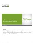
As is currently implemented in RISKMAN on a single stochastic run the system
shows:
The more varied line represents individual inter-annual Growth Rates and the less
varied line represents the Geometric Mean Growth Rates for all years up to that
point in the simulation.
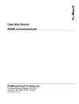
Therefore, for multiple runs the system shows:
The more varied solid line represents the average (i.e. the arithmetic mean) of
individual growth rates across the iterations, the dotted varied lines are the 1 (or 2)
SD lines on either side (depending on user setting). The less varied solid line
represents the average of the Geometric Mean Growth Rates across the iterations with
the “tapering off” dotted line showing the measure of dispersion. The “tapering off”
in the distribution of the Geometric Mean Growth Rates exists because the “mean of
means” has tighter distribution than sampled values do and the Geometric Mean
Growth Rate has more points and thus is more “stable” the later it is in the simulation.
Geometric Mean is only calculated based on runs not “exceeding criteria”.
19
RISKMAN
User Interface
User Interface
Overview
When RISKMAN is first installed it opens with a project “Default.prj”. You can
select any of the pre-installed projects by selecting the Open option in the File Menu
and searching in the “Projects” sub-directory.
During the normal course of operation the name of the last project used is stored in
the file “Riskman.ini” in the program directory and the last project is opened upon
start of the program.
Each time RISKMAN is launched, the Main Menu appears on the screen
accompanied by a series of graphs. The title bar at the top of the screen identifies the
program and displays the name of the project file that has been loaded. Users can
access all of the functions of RISKMAN through the Main Menu. Each of the
submenus and associated screens, fields and command buttons are described below.
The File Menu allows users to manage project files and create brief descriptions of
their contents. The Parameters Menu provides users with the opportunity to enter
data and modify biological parameters that will form the basis for model runs.
Results can be viewed, printed, exported and organized into customized reports from
the Output Menu. The Options Menu allows users to select and clear graphs,
identify project defaults, mode of operation (i.e., the level of complexity required –
deterministic, stochastic) and the wildlife species to be modelled. Finally, the on-line
help system is available by selecting from among the options in the Help Menu.
File Menu
The File Menu contains the project file management and description options.
20
RISKMAN
User Interface
These file management options function as they do in any standard Windows
application; additional windows appear to facilitate file management operations.
The file menu may also contain the names of up to four files most recently used by
the program.
Open Project
Selecting the Open Project option from the File Menu activates the Open Project
screen. Prior to displaying the Open Projects dialog you will be asked to save any
changes to the currently open project.
The dialog box will initially open in the directory where the current project is saved.
Choose a project file from the list of existing projects displayed on this screen or type
the full project name into the File Name field. Click OK to open the chosen file or
Cancel to return to the Main Menu.
Projects created with previous versions of the system can be read into RISKMAN,
however, some of the parameters introduced in the system since the creation of the
project file may not be initialized as needed.
21
RISKMAN
User Interface
Save Project and Save Project As
To save a currently open project with its current name, choose the Save Project
option from the File Menu. Any changes made to the data, parameters, options or
preferences will be saved under the current file name, overwriting the contents of the
original file with that name.
If you wish to create a new project first locate and open an existing one that most
closely resembles the new scenario you wish to simulate, them save it under a new
name using the Save Project As option. The file can be saved in the default projects
directory or another user-selected directory. This option is useful when there are
many populations being considered, or when the user wishes to organize imported
files, exported files, or output files with the relevant projects.
Projects saved with your current version of the system may not be compatible with
the previous versions of the system as new enhancements occasionally require new
parameters to be saved in the project files. If an incompatible version of the project
file is encountered (i.e. created with a later version of RISKMAN), the system issues
a warning and does not load the file.
Click on OK to save the currently open file or Cancel to return to the Main Menu.
Project Description
The Description option activates a screen that allows users to enter descriptive text to
provide useful supplementary information about the current project file.
22
RISKMAN
User Interface
Enter a full title for the project in the Title field, identify the creator of the project file
in the Owner field and enter a brief textual description of the project file in the
Description field.
Exit
The Exit option in the File Menu will exit RISKMAN.
Parameters Menu
The Parameters Menu provides users with the opportunity to enter data and modify
the biological parameters that will form the basis of model runs.
Recruitment
Selecting the Recruitment option activates the Recruitment screen. The main
component of this screen is the Recruitment by Age table and its four layers of data on
the Rates, Standard Error, Carrying Capacity, and Shape Factor (KS) tabs.
23
RISKMAN
User Interface
The Rates tab displays the top layer of data and contains the values that define the
rate of recruitment in the population.
For example, a species with a maximum age of reproduction set to 20 and minimum
age of reproduction set to four will be represented by 17 rows of data in the
recruitment screen. The number of columns is determined by the maximum litter
size. The maximum litter size, the minimum and the maximum age of reproduction
are entered in the Species Definition screen. For example, the maximum litter size set
at 3 offspring, results in three Probability of Litter Size columns (abbreviated to Prob.
with X in the table) plus two additional columns, Mean Litter Size and Proportion of
Females with Litters (Propn. with Litters) on the far right of the table (use the
horizontal scroll bar to access these as required).
Enter or modify values in the Recruitment screens according to available knowledge
about the general biology of the species being modelled. Cells in the Probability of
Litter Size columns can be modified. Note that the values entered for any given age
class (i.e., row) must sum to 1.0. For example, a user may enter the following values
for 6-year old female bears with litters: 0.170 (17%) have single cubs, 0.460 (46%)
have twins, 0.370 (37%) have triplets. These three values add to 1.0 (100%). The
Mean Litter Size is calculated as a weighted average of values in the Probability of
Litter Size columns for each age class. The mean litter size values cannot be
modified.
The Proportion with Litters column (far right) values are the user supplied fractions
of the surviving available-to-mate females that produce litters. For species with
annual reproduction cycles, all adult females are considered available each year.
However, for species with extended maternal care (e.g., bears), females with
dependent offspring do not mate and are not “available”. The values for Proportion
24
RISKMAN
User Interface
with Litters only apply to the reproducing females who are available to mate. For
clarity, these values are not equivalent to mean natality rates corrected for litter size
except for annual birth pulse species.
The Recruitment screen also offers the options to Export, Import and define Strata as
well as to identify Density dependent relationships and view the Density Dependence
plot (DDPlot).
At the bottom of the Recruitment screen is a field in which users can specify the
Proportion of Males at Birth. In addition in Stochastic mode only, users must specify
a value for the Standard Error associated with the proportion of males at birth. The
Standard Error field will not display if Deterministic mode is selected in the
Preferences screen (Options Menu).
Individual Survival
The Individual Survival option in the Parameters Menu activates the Individual
Survival screen.
This screen provides users with the opportunity to enter/modify values that will
define the probability of survival for all age and encumbrance categories. Like the
Recruitment screen, the Individual Survival screen features four layers of data on the
Rates, Standard Error, Carrying Capacity, and Shape Factor (KS) tabs. It also has
five command buttons on the right hand side that allow users to Export and Import
matrices, define Strata, identify Density dependence relationships, and view the
density dependence plot (DDPlot).
25
RISKMAN
User Interface
At the bottom of the Individual Survival screen is a field in which users can specify
Litter Survival Rate. The litter survival rate entered here is applied to whole litters
and this is done before the system applies individual survival rates. The number of
values requested depends on the maximum age of offspring unable to survive on their
own. This feature would only be used when there is evidence that mortality occurs to
the whole litter, as in the case of total milk failure, or environmental conditions too
extreme for young. When the model is being run in Stochastic mode, users must also
specify a value for the Standard Error associated with litter survival rate. The
Standard Error field will not display if Deterministic mode is selected in the
Preferences screen (Options Menu).
Hunting Mortality
Selecting the Hunting Mortality option activates the Hunting Mortality screen. The
Hunting Mortality screen is available only if the user has selected Annual or Spring
and Fall for Hunting Seasons on the Species Definition screen.
If hunting has been defined to contain two seasons there is a pair of tabs labelled
"Spring" and "Fall" at the top of the Hunting Mortality screen. If there is only one
hunting season defined there is no tab selection present. The hunting seasons can be
chosen as the hunting option in the Species Definition screen (see the Options Menu).
Click on the appropriate tab to modify the hunting parameters.
26
RISKMAN
User Interface
The "Spring" and "Fall" hunting seasons can represent any two sources of human
induced mortality with different characteristics (e.g. Resident/Non-Resident harvest,
First Nations harvest, etc).
The Mortality Level section of the screen allows users to set the level of hunting
mortality by selecting one of three options: 1) designating the number of animals to
be killed each year, 2) the proportion of the initial population to be killed each year,
or 3) the proportion of the current population to be killed each year. Additional fields
are available for stochastic mode and the Phased In Quota.
The Relative Selectivity/Vulnerability section of the Hunting Mortality screen allows
users to include a measure of the relative likelihood of mortality by hunting for all
age class and encumbrance strata in their simulation. There are six command buttons
associated with this section of the screen: Import, Export, Strata, Normalize, Hunt
Data, and Batch.
There are three ways to establish the harvest selectivity/vulnerability array. The first
is to simply enter the relative likelihood values. The second is to import a
selectivity/vulnerability array using the Import function. The third is to create a
selectivity/vulnerability array (Create S-V on the Hunt Data screen) by comparing a
harvest data array with the standing age distribution (as specified by the Relative
Distribution of the Initial Population). The resulting selectivity/vulnerability array is
saved in the project file with the rest of the project parameters and is used in
simulations.
The Sample Size field at the bottom of the Relative Selectivity/Vulnerability table
shows only when the model is set to run in stochastic mode (see Preferences in the
Options Menu). It provides means to specify the degree of uncertainty in the values
in the selectivity/vulnerability matrix.
The numerical values in the Selectivity/Vulnerability matrix do not determine the
probability of harvest directly. Rather the values are relative, with high values
indicating a particular sex/age/family class is relatively more likely to be harvested
than a sex/age/family class with a low value. Typically some sex/age/family class
cells may be pooled as a stratum, with all of the values in a given stratum equal. If
all values in the selectivity/vulnerability array are equal, the harvest is proportional
to the relative abundance of the sex/age/family classes. If cells or strata in the
selectivity/vulnerability array are not equal the harvest is selective. The actual
distribution of the harvest is a function of both the relative abundance and the relative
selectivity/vulnerability of the sex/age/family classes. Thus the distribution of the
harvest varies dynamically as a selective harvest alters the population’s
sex/age/family class distribution.
The Normalize function allows resizing the total of the Selectivity/Vulnerability
values to the user defined value (e.g. total harvest). This may make it easier to
interpret the values within individual cells.
27
RISKMAN
User Interface
The following is a numerical example with two population strata, their
selectivity/vulnerability and the resulting harvest for deterministic runs (the harvest
value used is 10).
Population
S/V
Harvest
100
100
2.0
1.0
6.7
3.3
100
150
1.0
1.0
4.0
6.0
100
150
2.0
1.0
5.7
4.3
To enter relative likelihood of mortality values:
1. Start by defining the strata with which you wish to work; re-display the Relative
Selectivity/Vulnerability matrix in stratified grid format.
2. Enter relative probability of mortality by hunting values for each cell in the
resulting matrix.
3. Click on the Normalize command button to generate the actual numbers of
animals vulnerable to hunting mortality for each cell of the matrix. The sum of all
normalized values in the matrix will be equivalent to value entered for Number of
Animals in the Mortality Level section of the screen or another value provided.
Note: The numeric value of the cells entered in the Relative Selectivity/Vulnerability
matrix is unimportant. Hunting mortality values need only be an accurate reflection
of relative selectivity/vulnerability for all sex, age, and encumbrance groupings.
Both harvest and population can have fractional values in the deterministic mode, but
are whole numbers in stochastic mode.
Using the Unselective Harvest option is equivalent ot setting all the
selectivity/vulnerability values to 1.0. The original values are preserved in the project
file and can be restored by clearing the Unselective Harvest check box.
The Batch button allows you to specify a series of mortality level values, which will
be applied in sequence in successive simulation runs (deterministic or stochastic).
28
RISKMAN
User Interface
The Mean and the SE specified for the Hunting Mortality Batch can be related to the
Number of Animals, Proportion of Initial Population or Proportion of Censused
Population.
The Save Results for Each Run option tells the system to save full reports for each of
the runs into individual files named 'RISKREP_x.CSV' (where ‘x’ is the run number).
Information for additional runs can be added or removed using the Add and Delete
buttons.
A Batch option is also available through the Initial Population screen. Also see
Running the Model section for additional details on the Batch option.
Phased In Quota
The Phased in Quota option allows modifying the harvest values over the course of
the simulation.
There are two ways of specifying the changing quota. When the Phased in Quota is
set to Automatic the harvest value is changed gradually through linear interpolation
between the Initial and the Final value. For the Number of Animals option these
values are always rounded down to the nearest integer.
In the Manual mode a specific value must be entered for each year of the simulation.
The schedule of these values is accessible by clicking the Set button. The newly
entered values become means in the simulation run.
In stochastic runs the same standard error (entered on the main harvest form) is
applied to all of the quota values independently.
29
RISKMAN
User Interface
The Phased In Quota cannot be used in conjunction with the Batch option.
Application of Uncertainty
The Sample Size field at the bottom of the Relative Selectivity/Vulnerability table
shows only when the model is set to run in stochastic mode (see Preferences in the
Options Menu). Use the Sample Size field to specify the number of times
RISKMAN will sample from the Relative Selectivity/Vulnerability matrix in order to
build each of the distributions it will use in the stochastic run. The size of this
parameter determines the degree of deviation between the vulnerability/selectivity
distribution entered by the user and the one used in a stochastic run. The higher the
value of sample size the closer the derived matrix will be to the original. For example
for the sample size of 115 at the beginning of each iteration 115 “individuals” are
randomly allocated (multinomial allocation) in the selectivity/vulnerability matrix
specified by the user. The resulting distribution forms a new selectivity/vulnerability
matrix used for that iteration. Therefore, the higher the sample size the closer the
iteration-specific matrices are to the user specified matrix. With a small sample size
the matrix has a large variability.
The value of Parm SE is applied at the beginning of each iteration of the simulation.
The value of Parm SE is considered to be all part of the parameter uncertainty. None
of it is applied as environmental uncertainty.
The hunting mortality is calculated by first determining the number of animals to be
harvested either by using the number of animals provided by the user or multiplying
the specified rate by the initial or the standing population. Each animal is then
allocated to a specific sex/age/family status group randomly using multinomial
allocation.
If the resulting individual turns out to be a female carrying for dependent offspring,
the offspring also die. The final year offspring (ie. all offspring for annual breeders;
Age 1 for two year breeding cycle; and Age 2 for three year breeding cycle) are
30
RISKMAN
User Interface
generally able to survive on their own and are not considered to be under the care of
an adult female.
In some cases a young may be harvested while under the care of an adult female,
therefore, the encumbrance class of that female must be changed. To do so the model
randomly selects females with offspring and removes one of her offspring. For the
most senior encumbrance class some of the offspring do not have adults carrying for
them. The model randomly determines if the harvested offspring is under a care of an
adult female.
Dealing with Over-harvest
In a declining population scenario some segments of the population may become
over-harvested and may not be able to support requested harvest. For example, let’s
consider two population segments:
Population in the segment
Selectivity/Vulnerability
Harvest Weight
30
4
120
4
30
120
Since the harvest weights are equal for both population segments ideally we would
like the harvest to be equal for both segments, however, if the total harvest is too high
(say 10 individuals) this cannot be accomplished and the actual harvest would be:
Actual Harvest
6
4
In a population with two population segments calculating the proper shift of harvest is
easy. However, the situation becomes more complicated when more segments are
present (e.g. age and encumbrance classes).
Let’s consider three classes with total harvest of 15 individuals:
Population in the segment
Selectivity/Vulnerability
Harvest Weight
Initial Harvest Allocation
5
24
120
5
30
4
120
5
4
30
120
5
In the initial allocation the harvest is equal for all segments. During the first pass the
system notes that there is need to reallocate harvest from the first segment. The
harvest allocation for the second pass becomes:
Harvest Allocation
5.5
5.5
4
Please note that the over-harvest from the last category has been distributed equally to
the remaining population segments since the harvest weights are equal between them.
Shifting the harvest during the first pass has pushed the first segment into overharvest. Here again we have to shift the over-harvest. There is only one population
31
RISKMAN
User Interface
segment without the maximum allocation (the middle one); therefore, the overharvest is pushed to that population segment:
Final Harvest Allocation
5
6
4
Even though the initially we have tried to allocate the harvest equally between the
population segments we were unable to do so due to low levels of the population
within some of the population segments.
The system has two methods for handling the situation when the overall harvest
cannot be supported by the population. By default, the overall harvest is reduced to
the total vulnerable population (where Selectivity/Vulnerability is greater than 0).
Alternately, the user can select the End Run with unfilled harv option, on the Hunting
Mortality screen. This truncates the execution of these runs.
The approach described above is used for deterministic calculations. In the stochastic
case the individual animals are allocated one at a time, which requires an integer
value for the number of animals to be harvested. If the user specified harvest calls for
“partial” animals (e.g. as a result of the harvesting a proportion of the total number of
animals) the harvest number is randomly rounded up or down. For example, if the
harvest being called for is 14.3 animals, the actual harvest has 30% chance of being
15 and 70% chance of being 14).
Once the total number of harvested animals has been selected the Selectivity/
Vulnerability matrix is “randomized” as described in the Application of Uncertainty
section. The relative harvest weights are calculated by multiplying the randomized
S/V matrix by the current population for each population segment (age/encumbrance
class).
The system then uses the multinomial (Monte Carlo) allocation procedure to allocate
harvest to each population segment.
Sex Selective Harvest
The system has two ways of allocating harvest between sexes. The default way is
using the relative Selectivity/Vulnerability values (sums for all males and females) as
described above. The second is to use the sex selective harvest. In the latter mode
the system allocates a fixed proportion of the harvest to each of the sexes (the user
provides the proportion of the harvest which is to be allocated females, the rest are
allocated to males).
In a declining population scenario allocating the full requested harvest to each
category may not be possible. For example for a harvest of 10 individuals we may
have the following situation:
Sex
Population Size
Harvest Allocation Proportion
Harvest Allocation
Male
6
0.70
7
32
Female
7
0.30
3
RISKMAN
User Interface
In the above situation the population cannot support the requested harvest; therefore,
the male harvest is reduced to the maximum available. If the End Run with unfilled
harv option is selected this also ends the run.
Harvest Allocation
6
3
The harvest within each sex is allocated to age and encumbrance classes using the
relative Selectivity/Vulnerability values assigned by the user as described above.
Hunt Data
The Hunt Data button on the Hunting Mortality screen activates the Hunting Data
screen. This screen features a stratified Harvest Distribution matrix into which users
can enter actual hunting mortality (harvest) data for the species being modelled.
RISKMAN will use these numbers to calculate the values for the Relative
Selectivity/Vulnerability table. Clicking on the Create S-V command button will
invoke the calculation, which will include normalizing (proportion that the hunted
population is with respect to the total population in the stratum) based on the userdefined initial population distribution (see Initial Population screen). Upon
completion of the calculations the user will be returned to the Hunting Mortality
screen. Selectivity/vulnerability values are generated for the currently selected hunt
(spring or fall). The system only holds one set of hunting data at a time, i.e., if you
switch from “spring” to “fall” hunting, the hunting data will remain as entered for the
spring hunt until you modify them. To save multiple sets of hunting data, use
RISKMAN’s Export and Import features.
For convenience there is a Strata button on this screen. It allows the user to define
the strata to be used in the entry of the hunting data and in defining the selectivityvulnerability array. These strata will also be used for the S/V matrix of the currently
selected harvest.
The Import Pop button allows to import the population distribution matrix as the
hunting data array. Using the project’s population distribution matrix instead of
actual harvest data to calculate the selectivity/vulnerability is equivalent to using an
unselective harvest.
The option Update Sample Size to the Sum of All Elements in the Harvest Distribution
Matrix sums all elements on the Harvest Distribution matrix and places the value as
the Sample Size on the Harvest screen.
33
RISKMAN
User Interface
Note that use of the Hunting Data screen is optional; users should enter data in either
the Relative Selectivity/Vulnerability table or the Hunting Data screen, not both.
Other Mortality
The Other Mortality option in the Parameters Menu will activate the Other
Mortality screen. The screen is only available when the appropriate option is enabled
on the Species Definition screen
“Other mortality” could include non-hunting human-induced mortality, e.g. defence
and/or and road kills. Depending on the species, other mortality occurs either before
or after the Fall harvest (see the description for the Species Definition screen for
more details). Using “other mortality” allows the user up to three unique selective
mortality operations that are individually applied to the estimated annual kill for each
type.
This screen is similar to the Hunting Mortality screen, offering the same opportunities
to Import and Export data, to define Strata, to set Mortality Level, enter and
normalize Relative Selectivity/Vulnerability values, and identify the Sample Size (for
stochastic runs).
34
RISKMAN
User Interface
Options Unselective Harvest and Sex Selective Harvest work similarly to on the
Hunting Mortality screen.
Initial Population
The Initial Population option in the Parameters Menu will activate the Initial
Population screen. This screen describes the initial relative abundance of living
animals in all age classes and stratified encumbrance groupings that have been set by
the user (i.e., the standing age distribution).
The fields at the top of this screen provide information about the total number of
animals in the initial population. Use the Total Initial Population field to identify the
initial size of the population. The standard errors associated with total population are
required only for stochastic runs. All of the standard error is designated as parameter
uncertainty.
The Population Indicator allows a choice between the mean and median of the
population values generated during a stochastic run. The mean is calculated only
among the runs not “exceeding criteria” so it is not unusual to observe an increase in
the mean population growth rate over time. The median is calculated from among all
of the runs. The value of percentile (%ile) is required for calculation of and display
of stochastic dispersion. The percentile range is distributed evenly on both sides of
the median. The percentile range is displayed on the graphs when the Display
Stochastic Error option is enabled on the graph selection screen.
35
RISKMAN
User Interface
The thresholds for runs “exceeding criteria” can be specified as reaching below or
above a given value.
The threshold criteria setting “below” allows an opportunity to specify the size of the
population below which it is considered non-viable. There are two ways to specify
the unacceptable criteria. If the value is specified as a number the population will be
considered non-viable if it reaches below that value. If the value entered is relatively
close to the mean starting population size (e.g. extinct at 500 with 800 starting value
and 300 standard error) some of the stochastic runs may start with “unacceptable”
populations.
If the criteria threshold is entered as a proportion of the initial size, the fraction of the
runs that result in unacceptable value is calculated for every iteration of the run based
on the proportion specified and the iteration’s initial population size.
Optionally, the runs with non-viable populations can be terminated. All values after
the year of termination are set to 0.
A run can also be considered “exceeding criteria” if it reaches above the specified
number or proportion. This specification can be used to test population recovery
scenarios. All options work similarly to the “below” setting.
36
RISKMAN
User Interface
The Relative Distribution section of the Initial Population screen features a matrix
that contains unstratified age and encumbrance classes. The number of rows (age
classes) depends on the maximum life expectancy of the species being modelled
(from the Species Definition screen in the Options Menu). The Sample Size field at
the bottom of this matrix shows only when the model is set to run in stochastic mode
(see Preferences in the Options Menu). Use the sample size field to specify the
number of times RISKMAN will sample from the Relative Distribution matrix in
order to build each of the distributions it will use in the stochastic run. This step is
similar to the use of uncertainty in the Hunting Mortality.
Enter relative abundance values into the matrix (as was the case with the hunting
mortality data, magnitude is unimportant) and click on the Normalize command
button if you wish to generate values based on the user-defined total initial
population.
A simulation run can be terminated if the population reaches a specified multiple of
the initial size. This feature prevents an apparent “stall” which occurs for large
potentially exponentially growing populations. The stall is due to RISKMAN
performing stochastic calculations for each individual, which may take a long time
for large populations.
The Start with the stable age distribution option at the bottom of the Initial
Population screen allows users to start a simulation run with a stable age population
calculated by the system. The calculations incorporate all recruitment and individual
survival data entered by the user, and excludes hunting and other (non-natural)
mortality. The calculation will run for 100 years, resulting in the distribution to be
used as the starting point for the simulation run. Following such a 100-year
calculation run, the system will re-set the total initial population to match what had
been entered by the user in the Total Population field of the Initial Population screen.
This option can be used to run comparative runs starting with stable and the entered
population distribution.
A similar effect can be accomplished by clicking the Stable Age button. This
replaces the values entered in the Relative Distribution table with the stable age
distribution calculated as described above. The distribution is normalized to the size
of the Total Initial Population. However, this distribution will be saved with the
project file.
The Initial Population screen also features Import and Export capabilities that
function as described for the other screens.
37
RISKMAN
User Interface
The Batch button allows you to specify a series of threshold setting for runs
“exceeding criteria”, which will be applied in sequence during a batch run. A batch
option is also available for the Hunting Mortality. Also, see Running the Model
section for more details on the Batch option.
The Save Results for Each Run option tells the system to save full reports for each of
the runs into individual files named 'RISKREP_x.CSV' (where ‘x’ is the run number).
Output Menu
The Output Menu provides users with the opportunity to send graphs to the printer,
view and export results.
Print Graphs
The Print Graphs option in the Output Menu sends all graphs selected for display to
the Windows printer. The resulting hard copy includes the name of the project that
was printed and identifies the mode in which the model was run (e.g., Deterministic,
3-year Reproductive Cycle).
View
The View and the Spreadsheet Export menus contain the same sub-menus and give
access to the same data in two different ways.
38
RISKMAN
User Interface
From the View menu the user can immediately display the data on the screen using
either the Windows Notepad or a spreadsheet of choice (see the Preference option on
the Options menu). The Spreadsheet Export menu allows the user to write the data to
a user defined file in a CSV format (accessible from all major spreadsheet programs).
The options Initial, Stable and Final Population Structure allow review of the
population. The population matrix can either be viewed in the normalized (to 1000)
or non-normalized format (see the Preference option on the Options menu).
The Selectivity/Vulnerability Matrix option allows review of the Spring and Fall or
Annual matrix.
The Final Year Harvest Distribution Matrix option displays the mean and the
standard error of the harvest in the final year of the simulation. The mean only
includes data for stochastic runs not “exceeding criteria”.
The Indicator Summaries menu gives access to year-by-year mean, sum of squares,
standard deviation and standard error for all of the indicators defined for graphing.
At the end of the indicator summary there is the year-by-year median, lower and
upper percentile for the Male, Female, and Total population.
Indicator Individual Runs menu lists the values of indicators from up to the first 50
stochastic runs.
Unacceptable Run Summaries display the number and proportion of the runs
“exceeding criteria” for individual years of the simulation.
The Report displays the initial and final population structure followed by the
indicators.
Spreadsheet Export
The Spreadsheet Export option activates a screen that allows users to select run
results for one or more indicators and export them in comma and quote delimited
ASCII format suitable for importing into spreadsheet or database applications.
39
RISKMAN
User Interface
The submenus are the same as for the View menu described above.
RISKMAN Export
The RISKMAN Export function allows you to export population structure data
resulting from simulation runs in a format suitable for importing into other
RISKMAN screens.
This option allows using the stable or final age distribution as the initial state for
other runs. This makes it unnecessary to continue to recalculate the stable age
distribution every time you run the model. This is equivalent to clicking the Stable
Age button on Initial Population screen. It also allows to continue a run from the
last year simulated.
For example, if you wish to use the final population structure of the species being
modelled, start by running the simulation. Following the run, select RISKMAN
Export and Final Population Structure from the Options Menu. The export screen
offers the opportunity to select the file name. Return to the Initial Population screen,
click on the Import command button, select the file you have just exported and click
on OK. The values of the final population structure will be inserted into the initial
population matrix, overwriting the values that were there before.
Vital Rates Export
The Vital Rates Export function allows the system to export the Initial, Stable or
Final age distribution or the Final Year Harvest Distribution Matrix in a format
compatible to the Vital Rates system.
40
RISKMAN
User Interface
Vital Rates is a population analysis system for polar bears and other species with
three-year reproductive cycles. The Vital Rates system consists of two components:
Anursus and its companion program Interval. These two programs allow calculation
of the mean and standard error of population parameters for species with three years
of parental care (e.g., polar bears, grizzly bears, and walrus).
Options Menu
The Options Menu provides users with the ability to identify project defaults, mode
of operation (i.e., the level of complexity required) and the species to be modelled.
Preferences
Selecting the Preferences option from the Options Menu will activate the
Preferences screen. Here, users will identify project settings.
Currently, there are two run modes available in RISKMAN: Research-Deterministic
and Research-Stochastic. The Research-Stochastic mode is the most complex mode
and the most capable of mimicking the natural dynamics of populations. When
running the model in this mode, users will need to enter the number of Monte Carlo
trials they wish the model to execute during a run by entering a value in the Trials
field. The Research-Deterministic mode incorporates all of the aspects of the model
simulated in the stochastic mode except the dynamics associated with random
variation.
Some project files may be “locked” with a limited access to its parameters. These
projects are in a “Management Mode” and are mainly designed for ongoing use in
managing populations with few, if any, changes to the parameters.
41
RISKMAN
User Interface
The stochastic uncertainty is split into two types: the Parameter Uncertainty and the
Environmental Uncertainty. The parameter uncertainty is applied only once at the
beginning of each stochastic run. The environmental uncertainty is applied each year
of the simulation. Both types of uncertainty can be turned on or off and the Standard
Error can be apportioned between environmental and parameter uncertainty.
The allocation between the parameter and environmental uncertainty can be changed
by entering proportions or picking a value along a slide bar. The proportions set are
applied to all of the Standard Error values not allocated specifically to the parameter
uncertainty.
The results of the simulations can be viewed in two types of editors: the Notepad or a
user selected spreadsheet program.
Turning on the Prompt for Description on "Save As..." option box at the bottom of the
Preferences screen will activate the Project Description screen whenever the user
saves the project file under a new name.
42
RISKMAN
User Interface
The option Normalize the Male/Female Population Structures Before Viewing Output
enables or disables the normalization of matrices to the total population of 1000
before values are viewed or exported.
Species Definition
The Species Definition screen provides users with the opportunity to select speciesrelated parameters that will form the basis for the simulation.
Select the reproductive cycle appropriate for the species being modelled by turning on
one of three available choices: 1) annual model (suitable for species with an annual
reproductive cycle), 2) black bear (2-year cycle) or 3) polar/grizzly bear (3-year
cycle).
Identify the season(s) in which the modelled species will be exposed to hunting. The
Hunting Seasons section of the screen contains three options: 1) none (i.e., no
hunting), 2) annual, and 3) spring and fall.
The order of calculations varies depending on the species selected. For the annual
and the 2-year model it is as follows:
* Natural Mortality
* Aging
* Recruitment
* Spring Harvest
* Other Mortality (if enabled)
* Fall Harvest
For 3-year model the order is:
* Natural Mortality
* Aging
* Recruitment
* Spring Harvest
* Fall Harvest
* Other Mortality (if enabled)
43
RISKMAN
User Interface
The program can simulate other non-hunting mortality. This type of mortality can
optionally be turned on or off by clicking the Apply “Other” Mortality switch.
Enter the maximum age of individuals in the population to be modelled in the
Maximum Age field. The Calc. Reproductive Value for Age field allows users to enter
the age of a female for which they wish reproductive value to be calculated and
graphed. Reproductive value can be used to quantify the relative impact on
population growth rate of harvesting one particular age (or age strata) versus another
by calculating the “present value of future offspring” for that age class (Pianka 1978).
That value is generally highest for animals at the age of first reproduction.
The entered value for the age is also used for calculating data for the graph %
Females in Harvest and the graph Adult Male/Female Ratio.
To include density effects in the simulation run, turn on the Density Dependence
option in this screen. This switch will influence all screens on which density
relationships can be defined, i.e., when turned off, the Density and DDPlot command
buttons will disappear and the Carrying Capacity and Shape Factor data matrices will
be disabled.
Typically, density effects are modelled as the effect of total numbers on population
growth rate. However, the rationale for an age structured model is that not all
individuals (and most particularly not all females) contribute equally to population
growth. The mechanism of density effects can be social or nutritional reductions in
44
RISKMAN
User Interface
recruitment or survival rates of the various sex, age, and family status strata in a given
population. Similarly, it may be the density of only one stratum, or some subset of
the total population strata, that produce a density effect on the survival and
recruitment parameters of one stratum. The manner in which density affects survival
and recruitment may be unique for each stratum. RISKMAN allows the user to
specify which parameters of which strata are affected, and to identify which strata or
stratum caused each specific effect.
A population may be regulated by reductions to recruitment, survival or both. For
most harvested populations, the number of density effects options that could regulate
a population at a given level is unmanageably large. Eliminating silly options that are
inconsistent with the population’s biology still leaves a very large number of
possibilities. Given the difficulty of accurately measuring a population’s survival and
recruitment at a constant density, the difficulties of quantifying density effects over a
range of densities is prohibitive for most harvested populations. However, an
approach is suggested by the equation used to model density effects. If the affected
parameter (in the affected strata) is monitored over a range of densities, the “carrying
capacity” (CC), and “non-linearity” (KS) values can be estimated by non-linear
regression.
For most populations, the data required to identify and quantify the mechanism of
density effects will not be available. This is not a deficiency in the simulation model,
but rather it is a deficiency in understanding how populations are regulated. This
density effects option was developed both to incorporate information on density
effects, and to allow the user to game with the model and explore density effects
scenarios. When density effects are not included, the user should be aware that the
results are valid only for the range of densities that do not trigger density dependent
reductions in survival or recruitment (i.e., low to intermediate densities, depending on
the biology of the population), and for the density at which the parameter estimates
were made.
There is also an option on the Species Definition screen to turn on a Co-variance of
recruitment and survival rates option, because it is likely that variance in recruitment
and survival rates is correlated (e.g., a “bad” year would reduce both recruitment and
survival). When turned on, this option causes the system to synchronize the
environmental component of variance for recruitment and individual survival rates.
Synchronization of environmental variability is accomplished by using the same
random deviate for all parameters in a given year. The parameter uncertainty is
considered to be entirely due to sampling error and thus is independent. The
alternative (i.e., independent parameters) is modelled by drawing a different random
deviate for each parameter each year. RISKMAN is an individual based model in
stochastic mode. Demographic uncertainty is modelled using Bernoulli trials.
In the Recruitment section of the Species Definition screen, users define Maximum
Litter Size, Minimum Age of Reproduction and Maximum Age of Reproduction.
These values set the boundaries for the Recruitment by Age matrix of the Recruitment
screen (Parameters Menu) and directly influence strata defined by the user.
45
RISKMAN
User Interface
Note: When changes are made to any of the recruitment parameters in the Species
Definition screen, or to Maximum Age, existing strata become invalid and will
automatically be deleted (i.e., recruitment, individual survival, hunting mortality,
natural mortality).
Setup Graphs
The Setup Graphs option in the Output Menu activates the Setup Graphs screen.
With this screen, users can select indicators to be graphed, a subset of lines for those
indicators, set numerical boundaries for the Y axis and identify formatting
preferences.
The Indicator column of the Setup Graphs screen lists all the indicators available for
graphing. Each of the eight rows in this column contain a full list of indicators,
available in a drop-down list.
Select the indicator to be graphed by simply highlighting the choice with a click of
the mouse. Each of the indicators has up to four lines that describe it. You can select
a subset of those lines by clicking on the Sub button. The indicator chosen will
dictate the setup of the Y axis. The columns labelled Y Minimum, Y Maximum and Y
Ticks allow users to select range and tick interval values to be displayed on the Y
axis. For example, setting Y Minimum = 0, Y Maximum = 80 and Y Ticks = 4
generates a graph with a Y axis displaying ticks (and values) every 20 places from 0
to 80. Alternatively, users can instruct RISKMAN to select the Y axis parameters by
clicking on the Dynamic Y Axis option box.
46
RISKMAN
User Interface
The X axis for each graph shows the number of years being simulated in the current
run. Choose whether or not to display values and ticks on the X axis by clicking on
the X Axis Labels option box in the next column.
The Visible column on the far right of the Setup Graphs screen allows users to select
which graphs they wish to see displayed with the Main Menu screen when the system
is launched. The system can display from one to eight graphs at the same time.
At the bottom of the screen the user has an opportunity to choose to display stochastic
error (this option is only available in the stochastic mode). The user also has a choice
to display the error as a line with one or two standard deviations (Std Dev) or
Standard Errors (Std Error) away from the mean. A standard error is a measure of
dispersion of means of distributions of observations while the standard deviation
measures observations themselves.
The Overlay option cannot be used while the stochastic variability (SD/SE) is
displayed on the graphs. When the SD/SE is off you can use runs with a single or a
small number of iterations to visually gauge the degree of variability in the results
caused by the current set of parameters.
The central tendency and the variability characteristic for the total population can also
be displayed as a median and a percentile by making the appropriate choice on the
Initial Population screen. The settings there will overwrite the values selected here,
but only for the population panel.
For long stochastic runs it may be worth displaying a “preview” of the results using
the Display Stochastic Run Preview option. A summary of the results of the first 10%
of the runs are displayed.
47
RISKMAN
User Interface
Colours and Line Styles
The Styles command button at the bottom of the Setup Graphs screen activates the
Colours and Line Styles screen with which users can customize the appearance of
their graphs.
Here you can select different colours and line attributes for up to four graph lines per
graph.
Help Menu
Windows Help offers a quick way to find information, such as how to perform a
particular task. Within a Help topic there may be one or more jumps or pop-up links
which you can click to display additional information about the topic. The mouse
pointer changes from an arrow to a pointing finger when it is over a link. Simply click
on any link to activate it.
Jumps to tables or figures within the body of the text will display a secondary
window in which the table or figure will appear, with the original window remaining
visible. You can click on the x in the button in the upper right corner of a secondary
window to put it away, so that you can continue reading the original window.
In a button bar at the top of the Help main window, there are four command buttons:
Contents, Search, Back, Print, << and >>.
48
RISKMAN
User Interface
•
Contents returns you to the Contents topic page;
•
the Search command button activates a window that allows you to enter
keywords to search for help on a particular topic;
•
the Back command button displays the last topic viewed, moving back one topic
at a time in the order in which they were viewed;
•
use the Print command button to print the currently active Help topic;
•
use << and >> to move backward and forward in the "browse" sequence, which
is the sequence in which the author organized the text. You can use these buttons
to move through the documentation to read it as a conventional paper.
You can also move, resize, maximize, or minimize the Help window, just as you
would any other window.
Running the Model
In addition to displaying from one to eight graph panes at a time, the main window
displays several other options. Users can designate the number of years to run a
simulation by entering a value in the Years to Simulate field. The Overlay option
allows users to run up to four additional simulations (each with a different set of
recruitment, survival and/or mortality parameters but over the same number of years)
and have the results displayed along with those of the first run.
The Overlay option cannot be used while the stochastic variability (SD/SE) is
displayed on the graphs. When the SD/SE is off you can use runs with a single or a
small number of iterations to visually gauge the degree of variability in the results
caused by the current set of parameters.
49
RISKMAN
User Interface
The Run command button initiates the simulation run and generates graphs according
to the user’s instructions in Setup Graphs. The button’s description changes to
Interrupt for stochastic runs. Clicking this button instructs the system to complete the
current stochastic trial then stop. The number of years simulated up to the point of
interruption will appear in the Current Year box. Clicking on Run again will re-start
the simulation from the beginning rather than from the point of interruption.
Deterministic runs of the model cannot be interrupted.
Note: The results of simulation runs are not saved as part of the project files. To save
run results, use the options available in the Output Menu.
The Batch toggles allow the user to utilize a series of harvest levels (specified in
Hunting Mortality), and also utilize a series of criteria for runs “exceeding criteria”
(in Initial Population). This allows the user to explore a range of harvest values over
a range of acceptable outcomes in a single run. The probabilities may be defined as a
fraction of Monte Carlo simulations that exceed a given proportion of the initial
number, or a fraction of runs that are less than a stated proportion of the initial
number. Thus both recovery and decline scenarios can be evaluated. See description
for the Hunting Mortality screen and the Initial Population screen for details on the
two available batch options.
A large number of iterations is required when the distribution of outcomes are spread
out over time. The Batch options allow more efficient scheduling by identifying a set
of simulations that that are processed sequentially and automatically. The simulations
50
RISKMAN
User Interface
can run unsupervised over-night, or in the background. The results are saved in a
.CSV file to allow easy use in other programs or reports.
Display Graphs
Graphs are displayed in the space under the Main Menu bar.
For each graph shown on this screen, a legend listing all data points, and identifying
data groupings along with their associated line colours is accessible by doubleclicking anywhere on the graph pane.
51
RISKMAN
Schedule A
Schedule A
End User Licence
In consideration of the covenants of the End User Licensee in subsection (ii) below, Her Majesty the
Queen in right of Ontario as represented by the Minister of Natural Resources ("MNR") hereby grants
_________________________________ (the "End-User Licensee") a perpetual non-exclusive, nontransferable licence (the "End-User Licence") to use, copy, produce or re-produce the Enhanced
Software solely for research, development and wildlife management for the End-User Licensee's own
purposes, programs or operations; it being understood and agreed that:
(i)
the End-User Licensee shall have the right to make changes or enhancements (the "Enhancements") to
the Enhanced Software and the End-User Licence shall include and apply to any Enhancements; and for
the purposes of greater clarification, the End-User Licensee shall have the same rights to use such
Enhancements as it has to use the Enhanced Software;
(ii) all right, title, claim and interest, including without limitation any and all copyright, patent rights and all
other intellectual property rights in and to the Enhancements, including without limitation the source code
thereof, shall accrue to and vest solely and absolutely in MNR, and the End-User Licensee agrees to
execute such further written assurances to effect the aforesaid as may be required from time to time by
MNR, including without limitation an assignment of copyright in form and substance satisfactory to MNR
and MNR undertakes to make Enhancements available to end-users through an End-User Licence;
In consideration of the covenants of the End User Licensee in subsection (ii) below, Her Majesty the
Queen in right of Ontario as represented by the Minister of Natural Resources ("MNR") hereby grants
_________________________________ (the "End-User Licensee") a perpetual non-exclusive, nontransferable licence (the "End-User Licence") to use, copy, produce or re-produce the Enhanced
Software solely for research, development and wildlife management for the End-User Licensee's own
purposes, programs or operations; it being understood and agreed that:
(iii) the Licensee agrees to waive all of its moral rights as prescribed by the Federal Copyright Act in or to
the Enhancements in favour of MNR and to provide MNR with a written waiver of all such moral rights as
and when requested by MNR, from such End-User Licensee and from any parties whom such End-User
Licensee has caused or instructed or permitted to develop the Enhancements in whole or in part;
(iv) the End-User Licensee agrees to take the Enhanced Software "as is" without any warranty or
representation from MNR of any kind whatsoever;
(v) the End-User Licence is non-transferrable and the End-User Licensee agrees not to assign the End-User
Licence in whole or part without the express prior written consent of MNR;
52
RISKMAN
Schedule A
(vi) the End-User Licence shall not include any right to sell, market, licence or otherwise distribute or deal
with the Enhanced Software or any of the Enhancements and any such rights are hereby expressly
prohibited without the express prior written consent of MNR;
(vii) the End-User Licensee agrees to pay MNR a nominal End-User Licence fee in consideration of End-User
Licence administration and software distribution costs as MNR may from time to time determine;
(viii) MNR shall have the right to terminate any End-User Licence in the event of any breach thereof by the
End-User Licensee which is not duly rectified within 15 days of the End-User Licensee's receipt of written
notification from MNR of such breach.
(ix) the End-User Licence shall not include any right to use, incorporate or merge any portions of the
Enhanced Software with any Software other than the Enhanced Software and any of its Enhancements
and such rights are hereby expressly prohibited.
53
RISKMAN
Literature
Literature
References
Caughley, G. Analysis of Vertebrate Populations. John Wiley and Sons. 1997.
Cole L.C. Population consequences of life history phenomena, Quarterly Review of
Biology 29:103-134, 1954
Kalbfleisch, J.G., Probability and Statistical Inference, Volume 1: Probability, Second
Edition, Springer-Verlag, 1985
Law A. M., Kelton W. D., Simulation Modeling and Analysis, Second Edition,
McGraw-Hill, 1991.
Pianka R.P., Evolutionary Ecology, Second Edition, Harper and Row Publishers,
1978.
Taylor M.K., Cluff H.D., Managing the risk from hunting for the Viscount Melville
Sound bear population. Ursus 13:185-202, 2002
Taylor M.K., Kuc M., Obbard M., Cluff H.D., Pond B., RISKMAN: Risk Analysis
for Harvested Populations of Age Structured, Birth-Pulse Species
Thompson W.L., G.C. White, and C. Gowan. 1998. Monitoring Vertebrate
Populations. Academic Press. San Diego CA. 365 pp.
White, G.C. 2000. Population Viability Analysis: Data requirements and essential
analyses. In: L. Boitani and T. K. Fuller eds.; Research Technologies in Animal
Ecology: Controversies and Consequences. Columbia University Press. New York,
NY, 289-331 pp.
54
RISKMAN
Literature
RISKMAN Papers
Eastridge, R. and Clark, J.D. 2001. Evaluation of 2 soft-release techniques to
reintroduce black bears. Wildlife Society Bulletin 29: 1163-1174.
Howe, E. J. 2002. Population viability analysis for black bear (Ursus americanus) on
the Bruce Peninsula, Ontario, Canada. Unpubl. M. Sc. thesis, Trent University,
Peterborough, ON. 217p.
Taylor, M. K., Laake, J., Cluff, H. D., Ramsay, M., and Messier, F. 2002. The
Viscount Melville Sound polar bear (Ursus maritimus) population inventory. In press.
Ursus 11.
McLoughlin P.D, Managing Risks of Decline for Hunted Populations of Grizzly
Bears Given Uncertainties in Population Parameters, 2003
McLoughlin, P.D., Taylor, M.K., Cluff, H.D., Gau, R.J., Mulders, R., Case, R.L., and
Messier, F. 2003. Population viability of barren-ground grizzly bears in Nunavut and
the Northwest Territories. Arctic 56: 185-190.
McLoughlin, P.D., M. Taylor, M. Kuc, M. Obbard, H. D. Cluff, and B. Pond. 2004.
RISKMAN: Risk analysis for harvested populations of age structured, birth-pulse
species. Poster presentation 15th International Conference on Bear Research and
Management, San Diego, CA, 8-13 February 2004.
55
RISKMAN
Glossary of Terms
Glossary of Terms
Bernoulli trials
Random events characterised by 1) their results must be a success of failure,
2) the probability of success (or failure) must be the same for
all trials, 3) all trials must be independent from one another.
The probability of obtaining a given number of successes in a
given number of trials is represented by a binomial distribution.
56
RISKMAN
Index
G
Geometric Mean Growth Rate 18
Graphs
Colours 50
Data 53
Indicators 48
Indicators - subselection 49
Line Styles 50
Preview 50
Setup 48
Growth Rates 18
Implementation in RISKMAN 19
Index
A
Adult 46
Arithmetic Mean Growth Rate 18
H
B
Harmonic Mean Growth Rate 18
Help 51
Hunt Data 35
Hunting Mortality 28
Hunting Seasons 28, 45
Batch 53
Harvest 30
Population 40
Bernoulli 17
Bernoulli trials 16
Binomial 17
Blocking Multiple Cells 4
I
Import
Matrix 5
Individual Survival 27
Initial Population 37
C
Carrying Capacity 11
Colours 50
Compatibility 23, 24
Co-variance 18, 48
L
Licence 54
Life Table Matrices See Matrix
Definition 3
Line Styles 50
Litter (Whole Litters) Survival 28
Litter Probability 26
Litter Size 26
Densitity Dependence 15
Locked Projects 44
D
Density Dependence
Defining Relationships - example 13
Definition 10
Effect on Litter Size 15
Interface 12
On/off switch 47
Plot 14
Species Definition 47
Dependent Variable Strata 13
Deterministic 43
M
Main Menu 22
Management Mode 44
Matrix
Blocking Multiple Cells 4
Entering and modifying values 4
Export 5
Export RISKMAN results 5
Import 5
Import RISKMAN results 5
Life Table Matrices See Life Table Matrices
Maximum Age 46
Michaelis-Menton equation 11, 12
Monte Carlo 16
E
End User Licence 54
Export
Matrix 5
F
File Menu 22
Final Age Distribution 42
Full Grid 8
57
RISKMAN
Index
Species Definition 45
Recruitment 48
Spreadsheet Export 41, 42
Stable age distribution 39
Stalling Runs 39
Standard Deviation 50
Standard Error 50
Stochastic 43
Strata
Creating strata 6
Definition 6
Editing existing strata 7
Non-contiguous cells - example 7
Population 12
Stratified Grid 8
Styles 50
Survival 27
multinomial 32
Multinomial 16, 32
N
Natural Survival 27
O
Open Project 23
Order of calculations 45
Other Mortality 36, 46
Overharvest 33
Over-harvest 33
Overlay 52
P
Papers 57
Parameters Menu 25
Parm SE
Harvest 32
Phased In Quota 31
Population Strata 12
Preferences 43
Print Graphs 40
Project Description 24
T
truncation-for-symmetry 18
U
Uncertainty
Demographic 16
Environmental 4, 16, 44
Harvest 32
Parameter 4, 16, 44
Partitioning 17
Unselective Harvest 30
R
Recruitment 25, 48
References 56
Reproductive Cycle 45
Reproductive Value 46
RISKMAN
Uses 1
RISKMAN Export 42
RISKMAN.INI 22
Run command 52
Running the Model 52
Runs "exceeding criteria" 16, 21, 37, 40
V
Variance 16
Viewing Results 41, 44
Vital Rates Export 43
S
Sample Size 32, 35
Save Project 24
Save Project As 24
Selectivity/Vulnerability 32
Generating from Hunt Data 35
Hunt Data 7
Hunting - entry 29
Population effect on harvest 30
Sex Ratio 27
Sex Selective Harvest 34
Sex Selectivity 34
Shape Factor 11
58