Download Doc-To-Help Standard Template

OptiRisk Systems
SAMPL/SPInE
User Manual
Written by Christian Valente, supported by Gautam Mitra, Victor Zviarovich, Patrick Valente,Chandra Poojari,
Frank Ellison, Nico Di Domenica
OptiRisk Systems
Copyright © 1985-2009 OptiRisk Systems
DO NOT DUPLICATE WITHOUT PERMISSION
All brand names, product names, are trademarks or registered trademarks of their respective holders.
The material presented in this paper is subject to change without prior notice and is intended for general information
only. The views of the authors expressed in this paper do not represent the views and/or opinions of OptiRisk
Systems.
OptiRisk Systems
1 Oxford Road
Uxbridge
Middlesex
UB8 3PH
United Kingdom
www.optirisk-systems.com
+44-(0)1895-256484
Contents
1.
Acknowledgement of Contributions
5
2.
Scope and Purpose
7
2.1
2.2
The Context ...........................................................................................................7
Cross Reference to Documents..............................................................................7
3.
Directed Reading
4.
Installation and Licensing
4.1
4.2
5.
6.3
7.2
SPInE User Manual
15
Using SAMPL ..................................................................................................... 15
Menu Items .......................................................................................................... 15
Stochastic menu ................................................................................................... 15
Dialog boxes ........................................................................................................ 16
Generator options ................................................................................................ 17
Solver Options ..................................................................................................... 18
Reporting Options ............................................................................................... 20
23
How to represent SP models ................................................................................ 23
Underlying deterministic model .......................................................................... 24
Declaration of the random structure .................................................................... 24
Tutorial 1: The Newsboy Problem ...................................................................... 25
A deterministic formulation................................................................................. 25
Implementing and solving the model in AMPL. ................................................. 27
The Newsboy Problem with uncertain demand ................................................... 29
Newsboy problem investigation with SAMPL .................................................... 32
Stochastic Extensions to AMPL: reference
8.1
8.2
8.3
8.4
8.5
8.6
12
Background ......................................................................................................... 12
Limitations of Deterministic Models ................................................................... 12
Understanding the Problem ................................................................................. 13
Introducing Probabilities ..................................................................................... 13
Modelling with SAMPL
7.1
8.
Installation ........................................................................................................... 11
Licensing ............................................................................................................. 11
The SAMPL environment
6.1
6.2
7.
11
Introduction to Stochastic Programming
5.1
5.2
5.3
5.4
6.
9
35
Introduction ......................................................................................................... 35
Stages .................................................................................................................. 35
Scenario ............................................................................................................... 36
Probabilities ......................................................................................................... 36
Random Data ....................................................................................................... 36
Chance constraints ............................................................................................... 38
Acknowledgement of Contributions  3
8.7
8.8
9.
Tutorial (2): The Dakota problem
9.1
9.2
9.3
9.4
9.5
9.6
9.7
10.
10.5
10.6
10.7
10.8
10.9
11.4
53
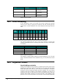
Problem statement ...............................................................................................53
Data modelling ....................................................................................................54
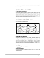
Algebraic model ..................................................................................................54
Implementing the model ......................................................................................56
Overview .............................................................................................................56
The underlying deterministic model ....................................................................56
AMPL formulation of the underlying deterministic model .................................56
Stochastic Programming Formulation .................................................................57
Model formulation ...............................................................................................58
Generate the SMPS instance ................................................................................59
Solving the model ................................................................................................60
Report the results .................................................................................................60
Analyse the results ...............................................................................................61
63
SAMPL architecture overview ............................................................................63
SP Generator Options (SPG) ...............................................................................64
SP Solver Options (SPS). ....................................................................................67
Calling the Solver Executable from Command Line ...........................................69
Reporting Options (SPR) .....................................................................................72
Stochastic Programming Theory and Background
12.1
12.2
12.3
12.4
12.5
12.6
13.
Problem statement ...............................................................................................43
Formulation of the deterministic problem ...........................................................43
Stochastic Programming extension of Dakota .....................................................45
Model formulation (two stage recourse model) ...................................................45
Chance constrained problem in SAMPL .............................................................46
Problem with integrated chance constraints ........................................................47
Investigating the model using SAMPL ................................................................48
Controls and Options Reference
11.1
11.2
11.3
12.
43
Tutorial (3): Asset/Liability Management
10.1
10.2
10.3
10.4
11.
Integrated chance constraints ...............................................................................39
Scenario Tree .......................................................................................................40
74
Classification .......................................................................................................74
Distribution Problems ..........................................................................................75
The Expected Value Problem ..............................................................................75
Wait and See Problems ........................................................................................76
Stochastic Programming Problems with Recourse ..............................................76
Scenario based recourse problems .......................................................................78
Distribution based recourse problems..................................................................78
Chance-constrained problems ..............................................................................79
Integrated chance constraints ...............................................................................79
Stochastic Measures: EVPI and VSS...................................................................79
References
81
Appendix 1. SMPS data format
83
A1.1 Introduction ...............................................................................................................83
A1.2 SMPS standard ..........................................................................................................83
Appendix 2. A library of models in SAMPL
89
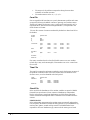
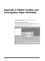
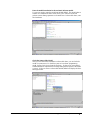
Appendix 3. Model Creation and Investigation Steps Illustrated
90
Scope and Purpose
SPInE User Manual
1. Acknowledgement of
Contributions
Stochastic programming extensions to AMPL: A Modelling Language for
Mathematical Programming is called SAMPL. SAMPL is embedded within a
stochastic programming modelling environment which is called SPInE. SAMPL
and SPInE follow on from SMPL and SPInE. These modelling and solver
systems have been researched by a number of researchers within CARISMA
(The Centre for the Analysis of Risk and Optimisation Modelling Applications)
under the guidance of Professor Gautam Mitra. The first version of
SMPL/SPInE was developed by Enza Messina and Francesco Fantauzzi with
solver work undertaken by Mr Frank Ellison. The next version SPML/SPInE
was developed mainly by Dr Patrick Valente supported by Dr Chandra Poojari
and Mr Frank Ellison in respect of the solver algorithms. Dr Patrick Valente,
Professor Gautam Mitra and Dr Mustapha Sadki are the principal designers of
SAMPL/SPInE. Professor Robert Fourer of Northwestern University and Dr
David Gay formerly of Lucent Technologies have provided input in the design
and realisations of SAMPL. We would like to thank Dr Cormac Lucas, although
he has not been directly involved in the design stage, his extensive testing of the
system and feedback have been very valuable.
P. Valente, G. Mitra, M Sadki
September 2004
Other Acknowledgements
SPInE User Manual

The Computational Optimisation and Modelling Group is now part of
CARISMA: The Centre for the Analysis of Risk and Optimisation
Modelling Applications, Brunel University, London (UK).

FortMP (TM), FortSP(TM), SAMPL (TM) are trademarks of UNICOM
consultants trading as OptiRisk Systems [4].

MPL (TM) is a trademark of Maximal Software Inc., USA [10].

CPLEX (TM) is a trademark of ILOG Inc [8].
Acknowledgement of Contributions  5
2. Scope and Purpose
2.1
The Context
This document is designed to serve both as a user guide and as a reference
manual.
We assume the user of the SAMPL system has a basic understanding of Linear
Programming (LP) and some experience of using a modelling system such as
AMPL (or MPL or OPL Studio) which is connected to an appropriate solver,
such as FortMP, CPLEX or MINOS. In this manual we first introduce basic
concepts of optimisation models under uncertainty, a natural extension of the
deterministic models where some or all the parameter values are uncertain.
A person new to the concept of stochastic programming should be able to use
SAMPL at a simple level after studying the introductory materials on stochastic
programming. However, this manual is not written as an introduction to
stochastic programming. Readers who require further explanation of stochastic
programming may first study our workshop notes [13].
At the modelling level, AMPL language has been enhanced with stochastic
programming constructs provided by SAMPL. In this manual it is also referred
to as stochastic extensions to SAMPL. A particular class of stochastic
programming problems, that is, the scenario based recourse models, is fully
supported by SAMPL. These two-stage and multistage recourse models can be
formulated using the SAMPL stochastic extensions and processed by the
stochastic solver embedded in SAMPL, which is called FortSP. The purpose of
this manual is to explain (a) modelling features (b) corresponding modelling
constructs and (c) solver controls necessary to process these models
2.2
Cross Reference to Documents
The user of SAMPL/SPInE should also refer to
(a) AMPL: A Modeling Language for Mathematical Programming
Prepared by Robert Fourer (Nortwestern University), David M Gay (AMPL
Opitmization LLC), Brian W Kernighan (Princeton University)
THOMPSONS, BROOKS, COLE, USA.
(b) AMPL STUDIO Manual:
Prepared by Kula Kularajan, Gautam Mitra, and Mustapha Sadki
(c) Stochastic Programming Lecture Notes, Copyright. CARISMA & OptiRisk
Systems.
(d) SMPL/SPInE, manual, Copyright. MAXIMAL Software and OptiRisk
Systems.
SPInE User Manual
Scope and Purpose  7
3. Directed Reading
The user of SAMPL first needs to go through the installation and licensing
procedure, which are explained in Chapter 4. Chapter 5 contains a simple
introduction to Stochastic Programming; a moderately knowledgeable user may
skip this chapter. On the other hand a novice user of stochastic programming
may first read the introductory Chapter 5, followed by Chapter 12. This may be
followed by an examination of the tutorial models presented in Chapter 7
(Tutorial 1: the Newsboy Problem) and in Chapter 9 (Tutorial 2: the Dakota
Problem). At this point the novice user may gain sufficient understanding of the
SP models to resume studying Chapter 6 of the manual.
By studying the menu options and the dialog boxes set out in Chapter 6, the user
will gain a broad understanding of the control structure and usage of SAMPL.
Chapter 7 explains of how to start modelling with SAMPL; in particular the role
of the underlying core LP model is discussed and the machine representation of
some of the key concepts of stochastic programming, scenario trees, stages,
scenario dimensions, probabilistic constraints and random data is introduced.
In section 7.2 and 7.3 the deterministic and stochastic version of the Newsboy
Problem are explained. The investigation of this model using SAMPL is set out
in section 7.4.
In Chapter 8 the stochastic extensions to AMPL are formally presented and the
user may return to this as a reference to the new language constructs.
In Chapter 9 a second tutorial is presented using the Dakota model, which is
kindly provided by Julia Higle and Stein W. Wallace [5]. This tutorial has three
sections covering the deterministic formulation, stochastic formulation and the
investigation using SAMPL. Some of the useful solver controls are also
explained in this Chapter.
In Chapter 10 the third tutorial is presented, which concerns the formulation of
an asset liability management (ALM) model.
The overall system architecture is first introduced in Chapter 11. The system
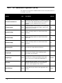
controls and options are also explained in this Chapter. The options are split into
three tables, each relating to a main functionality of SAMPL: Generation (SPG),
Solution (SPS) and Reporting (SPR).
Chapter 12 contains an overview of the main classes of stochastic programming
models.
There are two appendices in the manual. Appendix 1 contains an explanation of
the industry standard format SMPS used for the representation of stochastic
programming models, while Appendix 2 describes a library of SP models.
SPInE User Manual
Directed Reading  9
4. Installation and Licensing
SAMPL is a combined modelling and solver system for scenario based
stochastic programming problems with recourse also for chance constrained
problems [but very restricted scope]. The system is available as
(a) a stand alone application, as
(b) a run time dynamic link library and
(c) as an add-on to the AMPL modelling system in general and AMPLStudio in
particular.
4.1
Installation
<to be completed>
4.2
Licensing
<to be completed>
SPInE User Manual
Directed Reading  11
5. Introduction to Stochastic
Programming
5.1
Background
Optimisation models in general and linear and integer programming models in
particular have made considerable contribution to real world planning and
scheduling problems.
Unfortunately, their success has also showed up their limitations in many
situations where these models cannot be employed with any confidence. The
world of Linear Programming (LP) and Integer Programming (IP) models is
highly deterministic, and the underlying assumptions are that the parameters
which are used to define the models are known with fair certainty and perhaps do
not vary with time. In real life, however, these assumptions are not always true.
Stochastic Programming (SP) models tackle this problem by enabling the
decision makers to include uncertainty into their optimisation models.
5.2
Limitations of Deterministic Models
Deterministic models work perfectly well in many situations. For instance
consider:



scheduling of airlines and buses to predetermined timetable,
scheduling of crews who operate the above,
scheduling of vehicles which carry out delivery to retailers;
in all these cases deterministic assumptions are essential and adequate. OR
specialists who are used to teaching, model building, applying them to real
problems and then explaining these to the decision makers are aware of many
situations where deterministic approach is inadequate. Mulvey et al [12] explain
this rather lucidly in the following way:
"As taught in introductory OR/MS courses, the dual variable i corresponding to
the ith constraint indicates the rate of change in the optimal objective value as the
RHS of the ith constraint changes. A large dual variable signifies that the solution
is highly sensitive to changes in the RHS coefficient. A small dual variable
signifies a relatively insensitive solution to small data perturbations.
At this point, students often ask the difficult and sometimes embarrassing
question: What should we do if the solution is highly sensitive? Many, though
none completely satisfactory answers are possible. Some examples are the
following: 1) be careful to get the RHS demand value correct; 2) conduct a
marketing effort to reduce the uncertainty in customer demand by increasing
brand loyalty; 3) alert the user to the model's sensitivity; 4) make clear that the
Scope and Purpose
SPInE User Manual
model's recommendations depend upon the model's assumptions - one of which
states that the data coefficients are correct."
Consider for instance the operation planning problem of an electrical power
system. If we make assumptions about their availability, operating characteristics
and also about consumer demand, we can determine an optimal electricity
generation plan for the future. But the optimal solution will be optimal for only a
particular set of parameter values. At the time of implementing the optimal plan
the actual values may be different due to unplanned failures, weather changes
and so on. In a financial portfolio optimisation problem for instance we may note
down the price of equities (stocks) and their returns and consider these to be
known parameters. We can then construct an optimum portfolio planning model
which is deterministic in structure.
But as it is well known to anyone aware of the vagaries of the financial market,
the price and return for stocks vary considerably and the essential aspect of this
problem known as volatility is not captured by the deterministic model: in any
case no one would consider implementing the solution of a deterministic
portfolio optimisation model.
5.3
Understanding the Problem
One of the major aspects of model building and model investigation for a given
problem is to gain an understanding of the problem at hand.
Sensitivity Analysis: Situations where deterministic models prove to be
inadequate one can gain insight through sensitivity analysis. Thus cost
coefficients cj or the right hand side values bi or the matrix coefficients aij could
be varied according to their full range of possible values. But this analysis
considering a component at a time can answer the questions relating to the
uncertain value of parameters in a very limited way.
Scenario Analysis: In this approach the planner assumes that certain
combinations of possible values of uncertain parameters should be considered
together: such combinations are called scenarios and the model is solved for
different scenarios. The optimal solution decisions and the corresponding
objective function values are then aggregated in a heuristic way. Through this
line of investigation of a range of solutions, parameter sensitivities may be
highlighted and appropriate solution is decided in a heuristic way.
Stochastic Programming (SP) models address these shortcomings by considering
the distributions of the uncertain parameters. SP extends optimisation paradigm
to the domain of descriptive models and some comparison can be made with
simulation models which also provides insight by studying possible outcomes of
different inputs and aggregating the results. To gain an understanding, however,
we may seek answers to two questions:


5.4
What is an optimal policy for the underlying deterministic version of
the problem.
How much information about the probability distribution is required to
arrive at an optimum solution under uncertainty.
Introducing Probabilities
Uncertain aspects of a physical problem can be represented by introducing
probabilities in the decision model. This leads to a thorny question: should we
assume that the decision maker can state probability distributions and thereby
capture the uncertainty inherent in the physical problem? A loose but simple way
to proceed would be for the decision maker to assign non-negative numerical
weights to each possible event following typical rules:


SPInE User Manual
the weights add up to 1,
if an event is certain then its associated weight is 1,
Directed Reading  13

if A and B are mutually exclusive events then the weight for 'A or B'
equals the sum of the weights of the separate events A and B.

Since finding the right values for these probabilities or weights is essential to
constructing accurate uncertainty models, Wagner [17] recommends the
following:
".. as a pragmatic matter, essentially, you can utilize four approaches to obtain
these probability distributions:




Use introspection.
Employ historical data.
Find convenient approximations.
State descriptive axioms.
Most often you would apply two or more of these approaches in combination."
It is possible to delve into statistical decision theory, Bayesian analysis or the
more widely used notion and interpretation of relative frequency. In orientedoriented practical OR models it is perhaps more insightful to view probability
assessments as those reflecting the decision- maker's state of mind.
Scope and Purpose
SPInE User Manual
6. The SAMPL environment
6.1
Using SAMPL
The SAMPL add-on to AMPL takes advantage of the several features provided
by the AMPL Graphical User Interface. In particular, user can edit stochastic
programming models using the AMPL editor and then process them using the
commands provided by SAMPL, as described in the Menu Items section. For
more information on the usage of the AMPL‟s environment, refer to AMPL User
Manual.
6.2
Menu Items
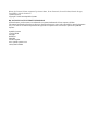
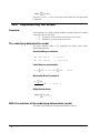
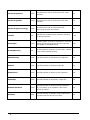
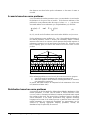
When integrated with the AMPL modelling environment, SAMPL provides the
system with a new menu item called Stochastic and a set of commands, which
enable the user to process stochastic programming models. The Stochastic menu
is displayed in Figure 1.
Figure 1. The Stochastic menu.
A description of the menu and the relating commands is set out below:
Stochastic menu
Check syntax
This command performs the syntax check of a model written using SAMPL‟s
extended AMPL keywords for stochastic programming.
SPInE User Manual
The SAMPL environment  15
Solve SAMPL
The current model is parsed, and then solved using SAMPL‟s solver. The solver
settings, including the solution types, can be modified using the Solver options…
command.
Generate SMPS
An SMPS representation of the current model instance is generated using this
command. By default, SAMPL/SPInE generates Windows/DOS text files. This
may not compatible with other UNIX based solvers. The advanced option
UnixOutput described in the SP Generator Options (SPG) section enables the
user to change the output text format to UNIX.
Solve Current
This command solves the latest SMPS instance generated for the current model.
If such instance is not available, then this command is equivalent to the Solve
SAMPL command.
Generator Options…
This command displays the Generator options dialog box. Settings for the
generator of SMPS instances can be modified using this command.
Solver Options…
This command displays the Solver Options dialog box. Settings for
SAMPL/SPInE‟ s solver can be modified using this command.
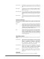
Reporting Options…
This command displays the Reporting Options dialog box. This dialog box
enables the users to change the way SAMPL/SPInE exports the solution vectors
obtained from the solver.
View Options list
This command displays the current settings of the SAMPL/SPInE system.
Advanced users can run this command in order to manually edit the advanced
options provided by SAMPL/SPInE.
View Scenario Tree
This command opens a graphic dialog box, which displays the structure of the
scenario tree associated with the current model.
6.3
Dialog boxes
The SAMPL/SPInE system provides a set of dialog boxes which enable the users
to set preferences for:



16  The SAMPL environment
The Generator of SMPS instances
The Solver
The Reporting tool
SPInE User Manual
Advanced options can be also set manually by editing the SAMPL options
list, which can be accessed using the View Options list command from the
Stochastic menu item.
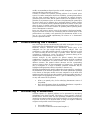
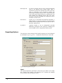
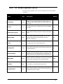
Generator options
The dialog box with the settings for the SMPS generator can be displayed by
selecting the Generator options… command from the Stochastic menu item.
Figure 2. SMPS Generator dialog
Model Stochasticity
These settings enable the system to optimise the generation of SMPS instances
by avoiding the processing of the model‟s coefficients, which are non random.
All models coefficients are considered random by default.
RHS:
if checked, the system assumes that the model contains
random Right Hand Side elements. Default is ON.
Cost Vector:
if checked, the system assumes that the model contains
random elements in the objective function. Default is ON.
Constraint Matrix: if checked, the system assumes that the constraint matrix
contains random elements. Default is ON.
Bounds:
if checked, the system assumes that the model contains
random bounds. Default is ON.
Generation Controls
These settings affect the algorithm used to generate the SMPS instance, as well
as the SMPS output.
Assume Constant Core: This option is disabled in the current version of SAMPL.
If unchecked, the generator examines each individual
scenarios in order to detect changes in the number of
variables or constraints in different scenarios. This process
may affect the speed of the generation process. In the
current SAMPL version, the individual scenario matrices
are assumed to have a constant number of rows and
columns. Default is therefore ON.
SPInE User Manual
The SAMPL environment  17
Compact SMPS:
If checked, the generator suppresses from the SMPS Stoch
file redundant elements. If an element appears in a scenario
with the same value as it appears in the parent scenario, then
that element is suppressed from the child scenario. Default
is OFF.
Scenarios
These settings enable the SMPS generator to process only a subset of the
model‟s scenarios, as well as scaling the probability vector.
Subset:
Indicates the number n of scenarios to be included in the
SMPS instance. Only the first n scenarios are added to the
SMPS output and their probability is automatically rescaled. If n=0 or n>S (where S is the total number of
scenarios as specified in the SCENARIO section of the
model) then all scenarios will be processed. Default is 0.
Normalise Probabilities: If checked, the system automatically re-scales the
probability vector if its elements do not add up to 1.
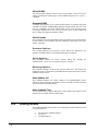
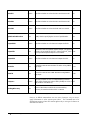
Solver Options
The dialog box with the settings for the Solver embedded in SAMPL can be
displayed by selecting the Solver options… command from the Stochastic menu
item.
Figure 3. Solver options dialog box.
Alternative Solutions
The solver is able to solve Here and Now, Wait and See and Expected Value
problems derived from the same Stochastic Programming model.
18  The SAMPL environment
SPInE User Manual
Here and Now:
If checked, the solver provides the solution to the Here and
Now (HN) problem associated with the model. Default is
ON.
Wait and See:
If checked, the solver provides the optimum objective
function values for all the scenarios associated with the
model. Default is ON.
Wait and See (full) (not yet implemented) If checked, the solver provides the
optimum objective function values for all the scenarios and
the solution values for all the first stage variables. Default is
OFF.
Expected Value:
If checked, the solver provides the solution to the Expected
Value (EV) problem associated with the model. Default is
ON.
Stochastic Measures
The solver is able to compute the Expected Value of Perfect Information (EVPI)
and the Value of Stochastic Solution (VSS) related to the model under
investigation.
EVPI:
if selected, the solver computes the value of the Expected
Value of Perfect Information. EVPI requires the solution of
both HN and WS models. Ticking this checkbox forces both
switches Here and Now and Wait and See to ON. EVPI is
calculated as the absolute difference between the WS
solution and the HN solution. Default is ON.
VSS:
if selected, the solver computes the Value of the Stochastic
Solution. VSS requires the solution of both HN and EV
models. Ticking this checkbox forces both switches Here
and Now and Expected Value to ON. VSS is calculated as
the absolute difference between the EV solution and the HN
solution. Default is ON.
Algorithms controls
These settings enable the user to control the execution of the solver, as well as its
output.
Algorithm Type:
this setting specifies the algorithm to be used for solving the
Here and Now model. HN models can be solved using
Benders‟
Decomposition
(Benders),
Deterministic
Equivalent with Implicit Non Anticipativity (DEQ Implicit)
and Deterministic Equivalent with Explicit Non
Anticipativity (DEQ Explicit). Default is Benders.
DEQ Algorithm:
Enables the user to specify the algorithm to be used for
solving HN problems via Deterministic Equivalent
approach. The available algorithms are Sparse Simplex
(SSX) and Interior Point Method (IPM). Default is SSX.
Stage filter:
Defines the highest stage-number st for which decisionvariables and constraints are to be output by the solver.
Default st=1.
Advanced
Advanced controls affect the inner execution of the solver‟ s algorithms.
SPInE User Manual
The SAMPL environment  19
First Stage VSS:
In order to calculate VSS we need to know the Expected
value of the expected value solution (EEV). EEV is
calculated by solving the expected value model, fixing the
result so obtained in the wait-and-see models, and
calculating the weighted objective value. Option First Stage
VSS can be used to restrict that the fix is performed to first
stage variables only (although in theory this is not correct
the result is often more meaningful as a complete fix may be
infeasible). Default is OFF.
Basis Restart:
Applies only to the Benders Decomposition algorithm, it
states whether in a leaf node repeats are solved using SSX
starting with the optimum basis from the previous run of
that node. Default is ON.
Use SPECS:
Specifies whether to use an independently provided
SPECS-file (fortmp.spc) when calling the underlying LP
solver FortMP to solve a sub-problem. Default is OFF.
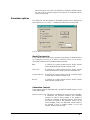
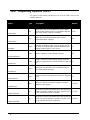
Reporting Options
The dialog box with the settings for the SAMPL reporting tool can be displayed
by selecting the Reporting options… command from the Stochastic menu item.
Figure 4. Reporting options dialog box.
Input
The reporter requires the specification of the solver type and the solver output
file, as well as the location of the dictionary file, containing the mapping
between SMPS names and algebraic names.
20  The SAMPL environment
SPInE User Manual
SAMPL solver:
This radio button specifies the SAMPL solver solution type.
It is selected by default and cannot be changed in the current
version of SAMPL.
OSL./SE:
This radio button specifies OSL/SE solution type. It is not
available in the current version of SAMPL.
Solution File:
This name identifies the solver output file. The default is
spinesol.sol.
Dictionary:
This textbox contains the name of the dictionary file used to
interpret the solver‟s output. The default is “*.dic”, where *
represents the full pathname of the current model without
extension.
Output
The reporter is capable of exporting the solutions to the stochastic model either
to text files or to database. These options enable the user to control the solution
reports.
Enable Text Output: if selected, the solutions for the HN, WS and EV models are
exported to individual text files. Default is ON.
EV output file:
specifies the name of the text file to which the solutions to
the EV problem will be exported. Default is “*_EV.sol”
WS output file:
specifies the name of the text file to which the solutions to
the WS problem will be exported. Default is “*_WS.sol”
HN output file:
specifies the name of the text file to which the solutions to
the HN problem will be exported. Default is “*_HN.sol”
Enable Database Output: if selected, the solutions for the HN, WS and EV
models are exported to a newly created database. Default is
OFF.
SPInE User Manual
DatabaseType:
enables the selection of the solution database type. Solutions
can be reported to Excel or Access. Default is Access.
DatabaseFile:
specifies the name of the database to be filled with the
solutions. If a database with that name exists, it will be
overwritten. Default is “*.mdb”.
The SAMPL environment  21
7. Modelling with SAMPL
7.1
How to represent SP models
The AMPL language extensions for stochastic programming provided by
SAMPL enable the user to define stochastic programming models in a simple
and concise way. The syntax of the extensions follows that of the AMPL
language. Together with the Definition Part and the Model Part that form an
AMPL model file, a new Stochastic Part is introduced, which contains a number
of sections identified by new keywords. The current extensions support the
definition of scenario based recourse problems, both two-stage and multistage
and chance constrained problems.
Future versions are expected to support also distribution based recourse
problems.
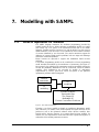
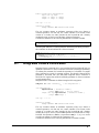
A Stochastic Programming model can be considered as a linear programming
model extended and refined by the introduction of uncertainty (see Figure 5).
More precisely, the underlying LP optimisation model is extended by taking into
account the probability distribution of the LP coefficients, which are random
variables. Such distributions are provided by models of randomness
(implemented in scenario generators), which are specific to the particular
optimisation problems under investigation.
Modelling of
random
parameters
SP
modelling
LP
modelling
Scenario Analysis
Expected Value
Two Stage RP
Multistage RP
Chance Constrained Problems
Figure 5. The combined paradigm
Therefore, it is always possible to identify an underlying deterministic model
(also called the core model). This model captures the logical structure of the
problem as well as the dynamical relations within decision variables, their
bounds and the objective function. In a scenario-based recourse problem, for
instance, the core represents the model associated with a particular sequence of
realisations of the random parameters (scenario).
SPInE User Manual
Modelling with  23
Underlying deterministic model
The definition of the underlying deterministic model makes use of the standard
constructs provided by the AMPL modelling. The core model could be linked to
the model of randomness in two ways:

Making variables, parameters and constraints explicitly parametric in
the scenario index
 Marking the appropriate coefficients as random parameters in such a
way that they can be treated implicitly.
The first approach requires that a scenario dimension must be introduced a priori
and precludes the possibility of describing models with continuous distributions;
it also implies the replications of variables and constraints. SAMPL adopts the
second approach, whereby one can write a pure deterministic model and use new
language constructs to identify the random parameters of the problem. Such
constructs also define the effects of the uncertainty on the underlying model
structure.
Declaration of the random structure
Once the underlying deterministic problem has been implemented, it is necessary
to merge it with the information related to the model of randomness, which
characterises the problem. We expand the language syntax in order to capture
such stochastic information. The items of information can be summarised as
follows:
Scenario Tree:
for scenario-based problems, it represents the structure
of the event tree.
Stages:
the time horizon of the underlying dynamic linear
program can be partitioned into decisional stages.
Scenarios probability:
the (discrete) probability distribution associated with
the scenarios.
Scenario dimension:
identifies a scenario index for scenario-based
problems.
Time dimension:
the index used to describe the temporal horizon in the
underlying model needs to be uniquely identified.
Random data:
defines and marks the random parameters of the
problem.
Probabilistic constraints: define chance and integrated chance constraints.
Extensions for
SP modelling
Standard AML
constructs
sufficient for the
definition of the
core models
Random
parameters
Stages
aggregations
Scenario tree
structure
Variables
Indices
Constraints
Time index
Scenario
index
Parameters
Objectives
Scenario
probabilities
Probabilistic
constraints
Figure 6. Extended language constructs
24  Modelling with
SPInE User Manual
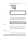
Figure 6 shows how the basic constructs of a modelling language for linear
programming are extended to capture the stochastic information. The design of
the new constructs is adapted to be consistent with the grammar of the
underlying AMPL modelling language. The parser of these AMPL language
extensions is the core of the modelling system embedded into SAMPL. This
system also generates data model instances in SMPS format and in a Stochastic
Intermediate Representation (SIR).
7.2
Tutorial 1: The Newsboy Problem
A deterministic formulation
The Informer, a newspaper having a wide circulation is interested in increasing
its efficiency in distribution. The company needs to decide, every day, what is
the optimal number of newspaper x to be printed in order to maximize the
profits. This, of course, depends on the demand D for the newspaper next day. In
this deterministic example, we assume that the company knows the demand with
certainty. Also, there is a limit on the amount of copies that can be printed, due
to the capacity of the lines. We indicate this by M. Each copy of the newspaper is
characterized by a unit selling price P = 90p and a unit printing cost of C = 81p.
Unsold copies e (i.e. copies printed in excess) represents a loss for the company.
Moreover, if the number of copies printed is less than the demand, the company
misses the opportunity to increase profits. We indicate this shortfall with h.
Shortfall and excess are only revealed once the demand is known, i.e. the day
after the copies have been printed. In stochastic programming jargon, this means
that x is a first stage variable, while e and h are second stage variables. We can
make this explicit by introducing a stage index as follows:
t=[1,2]
where t=1 indicates today and t=2 represents tomorrow.
This index can be defined in AMPL using the following declaration:
set time :=1..2;
The decision variables of the problem are therefore:
x t 1
ht  2
et  2
We can define the above decision variables in AMPL as:
var x{t in time: t=1}>=0;
var h{t in time: t=2}>=0;
var e{t in time: t=2}>=0;
For the time being, we assume that the company have managed to forecast an
exact value for the demand D=250. This parameter, together with the selling
price P the printing cost C and the maximum amount of printable copies M are
defined in AMPL as follows:
SPInE User Manual
Modelling with  25
param
param
param
param
p:=0.9;
C:=0.81;
D:=250;
M:=1000;
The total profit of the company is therefore given by.
max
profit  ( P  C ) xt 1  ( P  C )ht 2  Pet 2
In AMPL this expression can be written as:
maximize profit: sum{t in time:t =1}(x[t]*(P-C))
-sum{t in time:t=2}(h[t]*(P-C) + P*e[t]);
The number of copies, which can be printed, is limited by M. The following
constraint expresses this bound:
xt 1  M
which is equivalent to:
xt  M
for t=1.
This means that the constraint above is a first stage constraint.
In AMPL, this translates to:
subject to
Limit{t in time: t=1}: x[t]<=M;
The number of copies printed, the excess and shortfall of copies and the demand
are linked by the following balance constraint:
xt 1  ht 2  et 2  D
which can be rewritten as:
xt 1  ht  et  D
for t=2.
This second form explicitly states that the constraint can be verified when the
demand is revealed, in this case in the second stage. The constraint is therefore a
second stage constraint.
In AMPL, this translates to:
Balance{t in time: t=2}: x[t-1]+h[t] - e[t] = D;
To summarise, the problem above can be implemented in AMPL as follows.
26  Modelling with
SPInE User Manual
set time := 1..2;
param
param
param
param
P
C
D
M
:=
:=
:=
:=
0.9;
0.81;
250;
1000;
var x{t in time: t=1}>=0;
var h{t in time: t=2}>=0;
var e{t in time: t=2}>=0;
maximize profit: sum{t in time:t =1}(x[t]*(P-C)) -sum{t in time:
t=2}(h[t]*(P-C) + P*e[t]);
subject to
Limit{t in time: t=1}: x[t]<=M;
Balance{t in time: t=2}: x[t-1]+h[t] - e[t] = D;
Table 1. Informer model: deterministic formulation in AMPL.
Implementing and solving the model in AMPL.
The following steps explain the implementation and solution of the above
deterministic model using AMPL:
Start SAMPL and Create a New Model.
Start the SAMPL application, if you have not already started it, then choose New
from the File menu to create a new empty model file. Finally, choose Save As
from the File menu and save the file as informer.mod, for data related to the
model as informer.dat.
Enter the model formulation for the Informer model.
You are now ready to enter the model into the SAMPL. The model editor in
SAMPL is a standard text editor which allows you to enter the model and
perform various editing operations on the model text. In the model editor, enter
the formulation of Table 1.
Check the Syntax of the Model.
After you have entered the formulation in the model editor, you can check the
model for syntax errors. If SAMPL/SPInE finds a mistake in the formulation it
will report it in the Error Message window showing the erroneous line in the
model, along with a short explanation of the problem. The cursor is
automatically positioned at the mistake in the model file, with the offending
word highlighted.
To check the syntax at the model choose Check Syntax from the Run menu. If
there are no errors found SAMPL will respond with a message stating that the
syntax of the model is correct. If there is an error in the model SAMPL/SPInE
will display the Error Message window.
Solve the Model.
The next step is to solve the Informer model. Solving the model involves several
tasks for SAMPL/SPInE, including checking the syntax, parsing the model into
memory, transferring the model to the solver, solving the model and then
retrieving the solution from the solver and creating the solution file. All these
tasks are done transparently to the user when he chooses the solve command
from the menus. To solve the model follow these steps:
a.
b.
SPInE User Manual
Choose Solve FortMP from the Run menu or press the Run Solve
button in the Toolbar.
While solving the model the Status Window; appears providing
you with information about the solution progress.
Modelling with  27
If everything goes well SAMPL/SPInE will display the message “Optimal
Solution Found”. If there is an error message window with a syntax error,
please check the formulation you entered with the model detailed earlier in this
session.
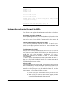
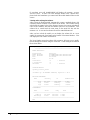
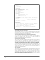
Viewing and Analysing the Solution.
After solving the model SAMPL automatically creates a standard solution file
containing various elements of the solution to the model. This includes among
other things the optimal value of the objective function, the activity and reduced
costs for the variables, and slack and shadow prices for the constraints. This
solution file is created with the same name as the model file but with the
extension .sol. In our case the solution file will be named Informer.sol.
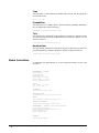
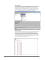
After you have solved the model you can display the solution file in a view
window by pressing the View button at the bottom of the Status Window. This
will display the view window shown below.
The View Window stores the solution file in memory, allowing you to quickly
browse through the solution using the scroll bars. A full listing of the solution
file is shown below.
AmplStudio Modeling System -Copyright (c) 2003 SM Software.
____________________________________________________________
MODEL.STATISTICS
Problem name
Model Filename
Data Filename
Date
Time
:Myproject
:Y:/AMPLStudio/Bin/informer.mod
:Y:/AMPLStudio/Bin/informer.dat
:10:6:2004
:11:40
Constraints
S_Constraints
Variables
: 2
: 1
: 3
:
Nonzeros
:
Nonzeros
SOLUTION.RESULT
Optimal_solution_found
'FortMP 3.2j: LP OPTIMAL SOLUTION, Objective = 22.5'
DECISION.VARIABLES
Name
Activity
.uc
Reduced Cost
________________________________________________________
x[1]
250.0000
1000.0000
0.0000
h[2]
0.0000
Infinity
-0.1800
e[2]
0.0000
Infinity
-0.8100
________________________________________________________
CONSTRAINTS
Name
Slack
body
dual
________________________________________________________
Limit[1]
750.0000
250.0000
0.0000
Balance[2]
0.0000
250.0000
0.0900
________________________________________________________
END
Table 2.Solutions to the informer deterministic problem
28  Modelling with
SPInE User Manual
The Newsboy Problem with uncertain demand
The deterministic version of the Informer model is not very useful in real life.
Obviously, the demand for the newspapers can be very different from the
estimated value, and the number of copies to be produced needs to take into
account this uncertainty. A stochastic programming approach gives us a solution
which explicitly takes into account the random parameters of the problem.
Scenario generation
In stochastic programming, the uncertainty of the random parameters is
introduced into the model by way of scenarios. A simple scenario generator for
the Informer model can be constructed as follows:
There are three sections of the newspaper: Economics, Sports and Politics.
Depending on the contents of each sections, people are more or less keen in
buying the newspaper. In particular, each section may contain good, average or
bad news. The following table shows how the contents influence the demand:
Contents
good
average
bad
Demand
195
150
70
Table 3. Newspaper demand dependency.
For instance, if each section contains good news the forecasted demand is
D=195+195+195=585.
The company then assigns a probability distribution to the contents of each
section of the newspaper:
good
average
bad
Politics Economics Sports
0.1
0.2
0.4
0.4
0.5
0.4
0.5
0.3
0.2
Table 4. Probabilities table
Assuming that the content of one section does not influence the contents of the
others (i.e. they are independent random variables), the company creates the
following table, which enumerates all possible combinations of the contents of
the three sections, with the relating demands. The probability associated with
each combination is given by the joint distribution of the individual section
contents:
Scen Politics
1bad
2average
3bad
4bad
5good
6bad
7bad
8average
9average
10bad
11good
12good
13average
14average
SPInE User Manual
Economics
bad
bad
average
bad
bad
good
bad
average
bad
average
average
bad
good
bad
Sports Probability Demand
bad
0.03
210
bad
0.024
290
bad
0.05
290
average
0.06
290
bad
0.006
335
bad
0.02
335
good
0.06
335
bad
0.04
370
average
0.048
370
average
0.1
370
bad
0.01
415
average
0.012
415
bad
0.016
415
good
0.048
415
Modelling with  29
15bad
16bad
17average
18good
19good
20bad
21good
22average
23average
24good
25good
26average
27good
good
average
average
good
bad
good
average
good
average
good
average
good
good
average
good
average
bad
good
good
average
average
good
average
good
good
good
0.04
0.1
0.08
0.004
0.012
0.04
0.02
0.032
0.08
0.008
0.02
0.032
0.008
415
415
450
460
460
460
495
495
495
540
540
540
585
Table 5. Enumerated scenarios
Each row of the table represents one possible scenario for the demand. In order
to reduce the computation, all the scenarios with the same value for the demand
are aggregated, and their probabilities are added up. This leads to the following
table, which contains the final scenarios used in the stochastic programming
problem.
Scen
1
2
3
4
5
6
7
8
9
10
Prob
0.03
0.134
0.086
0.188
0.226
0.08
0.056
0.132
0.06
0.008
Dem
210
290
335
370
415
450
460
495
540
585
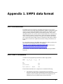
Table 6. Demand scenarios
The above table represents the probability distribution for the demand,
which is graphically illustrated in Figure 7.
Demand distribution
0.25
0.2
0.15
Probability
0.1
0.05
0
210 290 335 370 415 450 460 495 540 585
Figure 7. Distribution of the scenarios
30  Modelling with
SPInE User Manual
The demand parameter D of our problem becomes therefore a vector D[s], where
s represents the scenarios, with s =1..10; we also introduce a vector Prob[s],
which represents the probabilities associated with each scenario.
Formulation
The Scenario generation section illustrates how the company models the
uncertainty associated with the demand for the newspaper. In our example, there
are 10 scenarios for the demand. The stochastic programming version of the
Informer model requires therefore the definition of the scenario dimension. This
can be done with the following declaration:
scenarioset Scen;
We have shown that the demand parameter D is now a (random) vector indexed
over the scenario index. The declaration of D is removed from the DATA section.
In SAMPL, the random parameters of the problems are declared in the
RANDOM section. Considering Table 6, vector D can be declared as follows:
random param D{Scen} ;
Random data can be also read from database, as any other data vector in AMPL.
From Table 6 we also obtain the probabilities associated with the scenarios. We
declare a probability vector Prob[s] as follows:
probability param P{Scen};
and assign to it the values as we would do to any AMPL param:
param P :=
1
0.03
2
0.134
3
0.086
4
0.188
5
0.226
6
0.08
7
0.056
8
0.132
9
0.06
10 0.08;
The Informers model is a two stage recourse model. The scenario tree for a two
stage can be defined very easily using the extended AMPL constructs provided
by SAMPL:
tree theTree:= twostage{2};
For more information about the declaration of the tree structure associated with a
stochastic programming model, see the Tree section in the language reference.
To summarise, the stochastic programming version of the Informer model is
formulated as follows:
SPInE User Manual
Modelling with  31
set time;
scenarioset Scen;
tree theTree:= twostage{2};
param P := 0.9;
param C := 0.81;
param M := 1000;
random param D{Scen} ;
probability param P{Scen} := 1/card(Scen);
var x{t in time: t=1}>=0;
var h{t in time: t=2,Scen}>=0;
var e{t in time: t=2,Scen}>=0;
maximize profit: sum{t in time:t =1} (x[t]*(P-C)) -sum{t in time:
t=2} (h[t]*(P-C) + P*e[t]);
subject to
Limit{t in time: t=1}: x[t]<=M;
Balance{t in time: t=2,s in Scen}: x[t-1]+h[t] - e[t] = D[s];
Table 7. The Informer model formulated in MPL/SAMPL.
Newsboy problem investigation with SAMPL
The following steps explain the implementation and solution of the above
stochastic model using SAMPL:
Start SAMPL and Create a New Model.
Start the SAMPL application, if you have not already started it, and then choose
New from the File menu to create a new empty model file. Finally, choose Save
As from the File menu and save the file as informerSP.mod.
Enter the model formulation for the stochastic Informer model.
You are now ready to enter the model into SAMPL/SPInE. The model editor in
SAMPL is a standard text editor which allows you to enter the model and
perform various editing operations on the model text. In the model editor, enter
the formulation of Table 7.
Check the Syntax of the Model.
After you have entered the formulation in the model editor, you can check the
model for syntax errors. To check the syntax of a stochastic programming
model, choose Check Syntax from the Stochastic. If there are no errors found,
SAMPL/SPInE will respond with a message stating that the syntax of the model
is correct. If there is an error in the model SAMPL/SPInE will display the Error
Message window.
Solve the Model.
The next step is to solve the stochastic Informer model. Stochastic models are
solved using the stochastic solver embedded in SAMPL. To solve the informer
SP model, choose Solve SAMPL from the Stochastic menu. The solver can
produce the solutions to the Expected Value, Wait and See and Here and Now
problems, relating to the same model. For more information about SAMPL
solver‟ s settings refer to the Solver Options section of this manual.
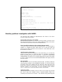
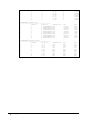
Analyse the results.
After solving the model, SAMPL creates one file for each solution type selected
(EV, HN or WS). Also, SAMPL creates a standard SAMPL solution file,
containing only the HN or EV solution. This includes among other things the
32  Modelling with
SPInE User Manual
optimal value of the objective function, the activity and reduced costs for the
variables, and slack and shadow prices for the constraints. This solution file is
created with the same name as the model file but with the extension .sol. In our
case the solution file will be named Informer.sol.
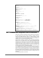
After you have solved the model you can display the standard SAMPL solution
file in a view window by pressing the View button at the bottom of the Status
Window. The SAMPL solution files, in our case InformerSP_HN.sol,
InformerSP_EV.sol and InformerSP_WS.sol can be opened choosing the Files
command from the View menu. Table 8 reports the contents of file
InformerSP_HN.sol
---------------------------------------------SAMPL SOLUTION REPORT
---------------------------------------------HERE AND NOW SOLUTION
Objective value: 14.4828
Algorithm: BEND
VARIABLES VECTOR: x
-----------------------------------------t
scenario
Activity
Bound
1
1
335
1
2
335
1
3
335
1
4
335
1
5
335
1
6
335
1
7
335
1
8
335
1
9
335
1
10
335
VARIABLES VECTOR: h
-----------------------------------------t
scenario
Activity
Bound
2
1
0
2
2
0
2
3
0
2
4
35
2
5
80
2
6
115
2
7
125
2
8
160
2
9
205
2
10
250
VARIABLES VECTOR: e
-----------------------------------------t
scenario
Activity
Bound
2
1
125
2
2
45
SPInE User Manual
Reduced Cost
Lower Bound
Upper
0
0
0
0
0
0
0
0
0
0
0
0
0
0
0
0
0
0
0
0
1e+036
1e+036
1e+036
1e+036
1e+036
1e+036
1e+036
1e+036
1e+036
1e+036
Reduced Cost
Lower Bound
Upper
-0.99
-0.99
-0.99
0
0
0
0
0
0
0
0
0
0
0
0
0
0
0
0
0
1e+036
1e+036
1e+036
1e+036
1e+036
1e+036
1e+036
1e+036
1e+036
1e+036
Reduced Cost
Lower Bound
Upper
0
0
0
0
1e+036
1e+036
Modelling with  33
2
2
2
2
2
2
2
2
3
4
5
6
7
8
9
10
1.13686837722e-0
0
-0.99
0
-0.99
0
-0.99
0
-0.99
0
-0.99
0
-0.99
0
-0.99
0
0
0
0
0
0
0
0
1e+036
1e+036
1e+036
1e+036
1e+036
1e+036
1e+036
1e+036
CONSTRAINTS VECTOR: Limit
-----------------------------------------t
scenario
Activity
Shadow Price
1
1
1.43954378222e-335
1
2
1.43954378222e-335
1
3
1.43954378222e-335
1
4
1.43954378222e-335
1
5
1.43954378222e-335
1
6
1.43954378222e-335
1
7
1.43954378222e-335
1
8
1.43954378222e-335
1
9
1.43954378222e-335
1
10
1.43954378222e-335
LHS
-1e+036
-1e+036
-1e+036
-1e+036
-1e+036
-1e+036
-1e+036
-1e+036
-1e+036
-1e+036
RHS
1000
1000
1000
1000
1000
1000
1000
1000
1000
1000
CONSTRAINTS VECTOR: Balance
-----------------------------------------t
scenario
Activity
2
1
-0.9
2
2
-0.9
2
3
-0.9
2
4
0.09
2
5
0.09
2
6
0.09
2
7
0.09
2
8
0.09
2
9
0.09
2
10
0.09
LHS
210
290
335
370
415
450
460
495
540
585
RHS
210
290
335
370
415
450
460
495
540
585
Shadow Price
210
290
335
370
415
450
460
495
540
585
Table 8. Here and Now solutions of the Informer SP model.
34  Modelling with
SPInE User Manual
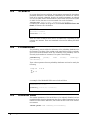
8. Stochastic Extensions
AMPL: reference
8.1
to
Introduction
The AMPL language extensions for stochastic programming provided by
SAMPL/SPInE enable the user to define stochastic programming models in a
simple and concise way. The syntax of the extensions follows that of the AMPL
language. With reference to the Definition and Model Parts that form an
AMPL model file, a new Stochastic Part is introduced, which contains a number
of sections identified by new keywords. The current extensions support the
definition of scenario based recourse problems, both two-stage and multistage.
In addition, chance constrained problems are easily accommodated.
Future versions are expected to support also distribution based recourse
problems.
8.2
Stages
This section allows the modeller to define the grouping of the decision variables
and constraints into stages. The staging is achieved by exploiting definition of
suffixes. A suffix can be considered as a generic property of a variable or
constraint, and can be used for our purpose to declare the stage which a variable
belongs to. The stage of the constraints is determined by the stage of the
variables which appear in it. The highest stage of any of such variables is the
stage of the constraint.
The syntax for the assignment of a stage number to a variable is very similar to
that of AMPL for other suffixes, but makes use of a predefined suffix called
stage:
suffix stage IN;
let indexingopt
name.stage := expr;
Alternatively, AMPL enables the suffix to be given in the variable declarations:
var name aliasopt indexingopt attributesopt, suffix stage
expr;
SPInE User Manual
Stochastic Extensions to AMPL: reference  35
8.3
Scenario
In scenario-based recourse problems, the uncertainty represented by the random
parameters introduces a new dimension, identified by the scenario set. This set
needs to be explicitly identified, because the random parameters are indexed
over it. The syntax used for the declaration of the scenario set follows the syntax
of AMPL for sets, but uses scenarioset instead of set in the declaration:
scenarioset name aliasopt indexingopt attribsopt ;
Considering the example model given in section Error! Reference source not
found., the scenario set is declared as:
param NS:=8;
…
#stochastic framework
…
scenarioset Sc:=1..NS;
…
There are certain conditions which have to be satisfied by S depending on the
scenarios tree structure. These are formulated in the section defining the TREE
keyword.
8.4
Probabilities
The probability section enables the declaration of the probability distribution for
the scenarios. The values of the weights can be retrieved from a file or explicitly
given in the model declaration itself. The cardinality of the probability vector is
obviously S (the number of scenarios). The syntax is the following:
probability
paramopt
attributesopt ;
name
aliasopt
indexingopt
These values represent a discrete probability distribution and need to satisfy the
following:
0  ps  1
S
p
s 1
s
s  1..S
1
An example of the PROBABILITIES section looks as follows:
…
scenarioset Sc:= 1..NS;
probability param Pr{Sc}:=1/card(Sc);
…
8.5
Random Data
The random parameters of the model have to be explicitly identified and are
treated differently from the deterministic data. Every random parameter has to be
indexed over the scenario dimension, which links the data vector to the scenario
tree structure.
random param name indexing attributesopt;
36  Modelling with
SPInE User Manual
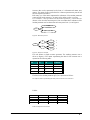
Scenario data can be represented in the form of a 2-dimensional matrix (tree
matrix). The matrix forms a grid where the columns represent time periods and
the rows represent scenarios.
Each entry (t,s) of the matrix represents the realisation of the random parameter
at time period t under scenario s. An entry can be either a scalar or a vector.
Let‟s consider a 3 time period horizon and random parameter p, which takes the
(known) value 10 in the first time period. Let us consider that 2 realisation of the
random parameter can be observed at each time period t=2..3, as in Figure 8:
p(t+1)=p(t)-50%
p(t)
p(t+1)=p(t)+50%
Figure 8. Binomial process.
5
10
15
2.5
1
7.5
2
7.5
3
22.5
4
Figure 9. Scenarios example.
This rule defines a simple scenario generator. The resulting scenario tree is
shown in Figure 9. The matrix representing the data for this scenario tree is
reported in the following table:
t=1
t=2
T=3
Scenario
10
5
2.5
1
10
5
7.5
2
10
15
7.5
3
10
15
22.5
4
The data for the random parameter p[T,S] are expressed as follows:
The (sparse) matrix representing the data for this scenario tree is shown in
Table 9:
t=1
10
t=2
5
15
t=3
2.5
7.5
7.5
22.5
s=1
s=2
s=3
s=4
Table 9.Compact scenario data.
SPInE User Manual
Stochastic Extensions to AMPL: reference  37
Such matrix can be represented in SAMPL in a row-wise fashion as:
#model file
scenarioset scen = 1..4;
random param dem{t,scen};
…
#data file
random param dem:=
1 1
10
2 1
5
2 3
15
3 1
2.5
3 2
7.5
3 3
7.5
3 4
22.5;
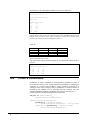
Although the data format here illustrated avoids any possible redundancy, it often
happens that the scenario data are provided in what we call expanded form. This can be
thought as the tree matrix above, where all entries are given. The expanded matrix
relative to the example previously investigated is shown in
Table 10:
t=1
10
t=2
5
15
t=3
2.5
7.5
7.5
22.5
s=1
s=2
s=3
s=4
Table 10. Expanded scenario data.
The data for the random parameter dem{T,S} are expressed in tabular form as
follows:
#data file
random param dem (tr):=
1
2
3
1
10
5
2.5
2
10
5
7.5
3
10
15
7.5
4
10
15
22.5;
8.6
Chance constraints
Probabilistic or chance constraints are characterised by randomness in some of
the coefficients and by a level β which indicates the probability of satisfying the
constraint. In a scenario-based problem a chance constraint is allowed to be
violated in some of the scenarios. Sum of probabilities of violated scenarios is
bounded by the reliability level β associated with the constraint. Since the
reliability parameter represents a probability it should be in the range [0, 1].
Chance constraints are defined using the following syntax:
subject to name indexingopt :
chance-constraint-expression ;
chance-constraint-expression:
probability { scenario-index :
basic-constraint-expression } rel-op cexpr
cexpr rel-op probability { scenario-index :
basic-constraint-expression }
38  Modelling with
SPInE User Manual
basic-constraint-expression:
expr rel-op expr
cexpr <= expr <= cexpr
cexpr >= expr >= cexpr
rel-op: = <= >=
scenario-index:
dummy-member in scenarioset-name
The expr construct denotes an arithmetic expression while cexpr denotes a
constant expression, one that may not contain variables. The scenario index
consists of a scenario set name preceded by the keyword in and a dummy
member the scope of which covers the basic constraint expression.
Consider the definition of the following deterministic constraint in AMPL
subject to SatisfyDemand{p in Prod}:
Produce[p] >= Demand[p];
Assuming that demand is a random parameter and defining reliability parameter
this constraint can be reformulated as a chance constraint
param Reliability = 0.6;
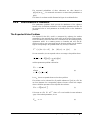
subject to SatisfyDemand {p in Prod}:
probability{s in Scen: Produce[p,s] >= Demand[p,s]}
>= Reliability;
8.7
Integrated chance constraints
Integrated chance constraints (ICC) were introduced by Klein Haneveld [18] as a
quantitative alternative to chance constraints. Instead of bounding the probability
of violating the constraint ICC bounds the expectation of a shortfall or a surplus
that is generated as a result of constraint violation. This bound is denoted by the
parameter β associated with each individual integrated chance constraint. It
should be non-negative but unlike the reliability parameter of chance constraints
it can be greater than 1.
Integrated chance constraints are defined using the following syntax:
subject to name indexingopt : icc-expression ;
icc-expression:
expectation { scenario-index }
( expr less expr ) rel-op cexpr
cexpr rel-op expectation { scenario-index }
( expr less expr )
rel-op: = <= >=
scenario-index:
dummy-member in scenarioset-name
The expr construct denotes an arithmetic expression while cexpr denotes a
constant expression, one that may not contain variables. The scenario index
consists of a scenario set name preceded by the keyword in and a dummy
member the scope of which covers the less-expression in brackets but not cexpr.
In AMPL the expression (a less b) is equivalent to max{a – b, 0}, so it can be
viewed as an amount of violation of the constraint a <= b.
Consider the definition of the following deterministic constraint in AMPL
SPInE User Manual
Stochastic Extensions to AMPL: reference  39
subject to SatisfyDemand{p in Prod}:
Produce[p] >= Demand[p];
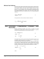
Assuming that the demand is a random parameter and defining the parameter
MaxExpShortfall this constraint can be reformulated as a chance constraint
param MaxExpShortfall = 100;
subject to SatisfyDemand{p in Prod}:
expectation{s in Scen} (Demand[p,s] less Produce[p,s])
<= MaxExpShortfall;
8.8
Scenario Tree
This section is of key importance, as it provides the modelling system with the
information related to the scenario tree structure. In a scenario-based problem,
the path can represent a scenario from the root node of this tree to one of the
leaves. Depending on the process that drives the scenario generation, different
ways of specifying this structure are allowed. It can be defined in the model
itself, it can be provided externally by the scenario generator, or it can be
retrieved in an automatic fashion from the scenario data.
tree
A tree is described in terms of time stages, as opposed to time periods. SAMPL
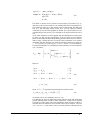
provides alternative ways of defining the tree structure. The syntax is as follows:
tree name:=opt tree_declaration ;
where <tree_declaration> one of:
bundle_list |
tlist |
nway{n}|
multibranch{n1, n2,...,nST}|
binary |
twostage {ns}opt ;
bundles
A compact representation of non standard trees can be obtained if one basic
assumption is true:
Scenarios are indexed in an order that ensures complete separation of all nested
sub-trees (i.e. the scenario paths never cross one another)
A <bundle_list> is defined as:
bundle_list : bundles{Bundle-1, Bundle-2,.. Bundle-n};
where:
Bundle-x: (stagex,scenx);
Each node of the tree has an associated bundle, which consists of the time period
in which the node lies, and a scenario number. The scenario number has to be
equal to the minimum of the ordinal values associated to the scenarios which
40  Modelling with
SPInE User Manual
pass through the same node. Figure 10 reports a scenario tree with non-standard
structure. The bundles representation follows.
1
2
3
4
1
2
3
4
5
6
7
8
9
Figure 10. Asymmetric scenario tree.
…
tree theTree:=
bundles
{
(1,1),
(2,1),(2,4),(2,6),
(3,1),(3,4),(3,6),(3,7),
(4,1),(4,2),(4,3),(4,4),(4,5),(4,6),(4,7)(4,8),(4,9)
};
tlist
Recalling the concept of tree matrix illustrated in the section dedicated to the
random keyword, a scenario tree can be represented as a list of S elements (tlist),
whose values are represented by the stage numbers where that scenario branches
from his father. A tlist can thus be constructed by considering the column
number associated to the leftmost element of each row of the tree matrix. As an
example, the tlist representing the scenario tree of figure 6 is the following:
tlist: tlist{n1, n2,.. nS};
As an example, the tlist representing the scenario tree is set out below:
…
tree theTree:= tlist {1,4,4,2,4,2,3,4,4};
…
nway{n}
In many applications, however, the scenario tree shows a "standard" structure:
this and the following keywords simplify the definition of trees with such
property.
Defines a tree where a constant number n branches occur at each stage σ=1..ST-1
where ST is the number of stages as implied by the STAGES section. The total
number of scenarios S of the problem has to satisfy the following equality:
S  n ST 1
multibranch{n1, n2,...,nST}
Defines a tree where at each stage σ=1..ST-1 is associated a number of branches
nσ. The NWAY tree is therefore a subclass of the MULTIBRANCH tree, whereby
SPInE User Manual
Stochastic Extensions to AMPL: reference  41
nσ is constant. The total number of scenarios S of the problem has to satisfy the
following equality:
ST 1
S   n
 1
binary
A binary tree is such that at each time stage, two possible outcomes of the
random data can be observed. The total number of scenarios S of the problem
has to satisfy the following equality:
S  2 ST 1
twostage
If the stagessection defines a two-stage aggregation or the model itself is twostage, then the tree is simply formulated using the twostage keyword. This is
equivalent to define an nway{S} tree, where S is the number of scenarios as
provided by the scenarioset section.
42  Modelling with
SPInE User Manual
9. Tutorial (2): The Dakota
problem
9.1
Problem statement
The following example was kindly provided by Julia Higle and Stein W.
Wallace [5]:
The Dakota Furniture Company manufactures desks, tables, and chairs. A desk
sells for $60, a table sells for $40, and a chair sells for $10. The manufacture of
each type of furniture requires lumber and two types of skilled labour: finishing
and carpentry. The cost of each resource and the resource levels required for
each item produced are given in Table 11 below.
Resource
Cost ($)
Production Requirements
Desk
Lumber (bd. ft.)
Finishing (hrs.)
Carpentry (hrs.)
Demand
2
4
5.2
8
4
2
150
Table
6
2
1.5
125
Chair
1
1.5
0.5
300
Table 11. Data for the Dakota problem
The combined questions of how much of each item should be produced, and the
level of resource required to meet this production can be addressed any number
of ways. Perhaps the easiest method is a simple per-item profit analysis. A desk
costs $42.40 to produce and sells for $60, for a net profit of $17.60 per item.
Similarly, a table costs $27.80 to produce and sells for $40, for a net profit of
$12.20 per item. That is, desks and tables are profitable. In the absence of any
constraints on resource availability, as Dakota works toward profit maximization
they should produce as many of these items as they can sell (i.e., 150 desks and
125 chairs). On the other hand, a chair costs $10.60 to produce and sells for
$10.00, for a net loss of $.60 per item. Based on the information provided, with a
view toward profit maximization Dakota should decline to produce any chairs.
9.2
Formulation of the deterministic problem
This deterministic model can be formulated in AMPL/SAMPL as follows:
SPInE User Manual
Tutorial (2): The Dakota problem  43
#SETS
set Prod;
set Resource;
#PARAMETERS
param Cost{Resource};
param ProdReq{Resource, Prod};
param Price{Prod};
param Budget;
param Demand{Prod};
#VARIABLES
var
Acquire{Resource} >=0;
var
Produce{Prod} >=0;
#OBJECTIVE
maximize Profit: sum{p in Prod} (Produce[p] *
Price[p]) sum {r in Resource}
(Acquire[r] * Cost[r]);
#CONSTRAINTS
subject to
c0{r in Resource}: Acquire[r]*Cost[r]<=Budget;
c1{p in Prod}: Produce[p] <= Demand[p];
c2{r in Resource}: Acquire[r] >=
sum{p in Prod} (Produce[p] *
ProdReq[r,p]);
Start SAMPL and Create a New Model.
Start the SAMPL application, if you have not already started it, then choose New
from the File menu to create a new empty model file. Finally, choose Save As
from the File menu and save the file as dakota.mod.
Enter the model formulation for the deterministic Dakota model.
You are now ready to enter the model into the SAMPL. The model editor in
SAMPL is a standard text editor which allows you to enter the model and
perform various editing operations on the model text.
Check the Syntax of the Model.
After you have entered the formulation in the model editor, you can check the
model for syntax errors. If SAMPL finds a mistake in the formulation it will
report it in the Error Message window showing the erroneous line in the model,
along with a short explanation of the problem. The cursor is automatically
positioned at the mistake in the model file, with the offending word highlighted.
To check the syntax at the model choose Check Syntax from the Run menu. If
there are no errors found SAMPL will respond with a message stating that the
syntax of the model is correct. If there is an error in the model SAMPL will
display the Error Message window.
Solve the Model.
The next step is to solve the Informer model. Solving the model involves several
tasks for SAMPL/SPInE, including checking the syntax, parsing the model into
memory, transferring the model to the solver, solving the model and then
retrieving the solution from the solver and creating the solution file. All these
tasks are done transparently to the user when he chooses the solve command
from the menus. To solve the model follow these steps:
44  Tutorial (2): The Dakota problem
SPInE User Manual
c.
d.
Choose Solve FortMP from the Run menu or press the Run Solve
button in the Toolbar.
While solving the model the Status Window; appears providing
you with information about the solution progress.
If everything goes well SAMPL/SPInE will display the message “Optimal
Solution Found”. If there is an error message window with a syntax error please
check the formulation you entered with the model detailed earlier in this session.
Viewing and Analysing the Solution.
After solving the model SAMPL/SPInE automatically creates a standard solution
file containing various elements of the solution to the model. This includes
among other things the optimal value of the objective function, the activity and
reduced costs for the variables, and slack and shadow prices for the constraints.
This solution file is created with the same name as the model file but with the
extension .sol. In our case the solution file will be named dakota.sol.
After you have solved the model you can display the solution file in a view
window by pressing the View button at the bottom of the Status Window. This
will display the view window shown below.
The View Window stores the solution file in memory, allowing you to quickly
browse through the solution using the scroll bars. A full listing of the solution
file is shown below.
9.3
Stochastic Programming extension of Dakota
Suppose now that the demands for products are uncertain, but that “low”, “most
likely”, and “high” values are available. In particular, suppose that the possible
demand scenarios are given in Table 12.
Item
Desks
Tables
Chairs
Probability
Low Value
50
20
200
0.3
Most Likely Value
150
110
225
0.4
High Value
250
250
500
0.3
Table 12.Uncertain demand.
We will assume that the low values occur with probability pl = 0.3, the most
likely values occur with probability pm= 0.4, and the high values will occur with
probability ph = 0.3. Notice that the set of possible demand scenarios and the
corresponding probabilities form a distribution that can be used to describe the
demand that Dakota might face in the future.
9.4
Model formulation (two stage recourse model)
Considering the stochastic constructs supported by SAMPL, the Dakota
stochastic programming model can be implemented as follows:
To illustrate the use of the new constructs for stochastic programming described
in the previous section, we modify the above deterministic model as follows:
SPInE User Manual
Tutorial (2): The Dakota problem  45
scenarioset Scen:=
1..NS;
“special” scenario set;
tree
theTree:= twostage{NS};
with NS scenarios
#declares
Scen
as
the
#declares a two stage tree
random param d{Prod,Deal,Time,Scen};
#declares demand as random
parameter
probability param Pr{Scen}:=1/card(Scen); #declares the probability
of the scenarios
suffix stage IN;
#assigns variables to stages
var x{Prod,Fact,Time,Scen}
else 2;
var y{Prod,Fact,Time,Scen}
else 2;
var z{Prod,Fact,Deal,Time,Scen}
else 2;
var w{Prod,Deal,Time,Scen}
else 2;
>=0, suffix stage if t=1 then 1
>=0, suffix stage if t=1 then 1
>=0, suffix stage if t=1 then 1
>=0, suffix stage if t=1 then 1
The set Scen is defined using the scenarioset keyword, which identifies it as a
special set. The tree keyword is used to define the structure of the scenario tree
as a two-stage (fan) tree.
The parameter d is declared using the random param keyword, while the
probability vector Pr is redefined as probability param. Finally, the variables are
partitioned into different stages by adding of the suffix stage to their definition.
Table 13. Model formulation using SAMPL stochastic extension for AMPL.
9.5
Chance constrained problem in SAMPL
The chance-constrained version of a modified Dakota problem is also formulated
using SAMPL. First we modify the problem by introducing a new second-stage
variable Sell that represents the amount of product sold. Two new constraints c3
and c4 restrict it to be not greater than the demand and the production level.
Objective is modified accordingly.
Let‟s now assume that in this model one of our goals is to satisfy the demand. To
reduce risk of producing too much and suffering losses under the worst scenario
we formulate the constraint as a chance constraint. In this small example
problem which contains only 3 scenarios with probabilities 0.3, 0.4 and 0.3 the
reliability level of 0.6 will allow the constraint to be violated at most in one
scenario.
So the underlying deterministic model is revised in the following way:
1. The Reliability parameter which represents β of equation ((18)) is added.
2.
The constraint c1 is declared as a chance constraint in the stochastic
framework.
The resulting model is set out below.
46  Tutorial (2): The Dakota problem
SPInE User Manual
#SETS
set Prod;
set Resource;
#PARAMETERS
param Cost{Resource};
param ProdReq{Resource, Prod};
param Price{Prod};
param Budget;
param NS = 3;
param Reliability = 0.6;
#SCENARIOS
scenarioset Scen = 1..NS;
tree ScenTree = twostage;
#RANDOM PARAMETERS
random param Demand{Prod, Scen};
#PROBABILITIES
probability P{Scen};
#VARIABLES
var Acquire{Resource} >= 0, suffix stage 1;
var Produce{Prod, Scen} >= 0, suffix stage 2;
var Sell{Prod, Scen} >= 0, suffix stage 2;
#OBJECTIVE
maximize Profit: sum{s in Scen} P[s] *
(sum{p in Prod} Sell[p,s] * Price[p] sum {r in Resource} Acquire[r] * Cost[r]);
#CONSTRAINTS
subject to c0{r in Resource}: Acquire[r] * Cost[r] <= Budget;
subject to c1{p in Prod}:
probability{s in Scen: Produce[p,s] >= Demand[p,s]}
>= Reliability;
subject to c2{r in Resource, s in Scen}: Acquire[r] >=
sum{p in Prod} Produce[p,s] * ProdReq[r,p];
subject to c3{p in Prod, s in Scen}: Sell[p,s] <= Demand[p,s];
subject to c4{p in Prod, s in Scen}: Sell[p,s] <= Produce[p,s];
9.6
Problem with integrated chance constraints
While chance constraints are appropriate for many problems they are qualitative
by nature meaning that only the fact that constraint is violated is taken into
account not the actual amount by which it is violated. However, a larger
violation is often disliked more than a smaller one. In this case integrated chance
constraints (ICC‟s) can be more appropriate because they are based on a
quantitative risk concept restricting the expected violation.
Another reason for using ICC‟s instead of chance constraints comes from the
fact that chance constrained problems are non-convex in general making them
difficult to solve. In order to solve chance constrained problems, FortSP
reformulates them as MIP problems with the number of binary variables in them
depending linearly on the number of scenarios. As a result only problems with
relatively small number of chance constraints and scenarios are computationally
tractable. On the other hand problems with ICC‟s can be solved efficiently using
either deterministic equivalent or cutting-plane methods.
Let‟s reformulate the chance constraint from the problem of the previous section
as an integrated chance constraint. To this end the Reliability parameter is
replaced with the MaxExpShortfall parameter which now can take values greater
than 1. To come up with the suitable value it is usually necessary to resolve a
problem several times with different settings of this parameter. Then observing
the resulting optimal values the modeller can choose an appropriate trade-off
between the objective value and the expected violation according to his/her own
preferences.
The reformulated problem is set out below.
SPInE User Manual
Tutorial (2): The Dakota problem  47
#SETS
set Prod;
set Resource;
#PARAMETERS
param Cost{Resource};
param ProdReq{Resource, Prod};
param Price{Prod};
param Budget;
param NS = 3;
param MaxExpShortfall = 100;
#SCENARIOS
scenarioset Scen = 1..NS;
tree ScenTree = twostage;
#RANDOM PARAMETERS
random param Demand{Prod, Scen};
#PROBABILITIES
probability P{Scen};
#VARIABLES
var Acquire{Resource} >= 0, suffix stage 1;
var Produce{Prod, Scen} >= 0, suffix stage 2;
var Sell{Prod, Scen} >= 0, suffix stage 2;
#OBJECTIVE
maximize Profit: sum{s in Scen} P[s] *
(sum{p in Prod} Sell[p,s] * Price[p] sum {r in Resource} Acquire[r] * Cost[r]);
#CONSTRAINTS
subject to c0{r in Resource}: Acquire[r] * Cost[r] <= Budget;
subject to c1{p in Prod}:
expectation{s in Scen} (Demand[p,s] less Produce[p,s])
<= MaxExpShortfall;
subject to c2{r in Resource, s in Scen}: Acquire[r] >=
sum{p in Prod} Produce[p,s] * ProdReq[r,p];
subject to c3{p in Prod, s in Scen}: Sell[p,s] <= Demand[p,s];
subject to c4{p in Prod, s in Scen}: Sell[p,s] <= Produce[p,s];
9.7
Investigating the model using SAMPL
In this tutorial the Dakota model will be first implemented, then solved and the
results exported to a MS Excel spreadsheet for further investigation.
Implementing the model
Start the AMPL application, if you have not already started it, and then choose
New from the File menu to create a new empty model file. Finally, choose Save
As from the File menu and save the file as DakotaSP.mod. You are now ready to
enter the model into SAMPL/SPInE. The model editor in SAMPL/SPInE is a
standard text editor which allows you to enter the model and perform various
editing operations on the model text. In the model editor, enter the formulation
of To illustrate the use of the new constructs for stochastic programming
described in the previous section, we modify the above deterministic model as
follows:
48  Tutorial (2): The Dakota problem
SPInE User Manual
scenarioset Scen:=
1..NS;
“special” scenario set;
tree
theTree:= twostage{NS};
with NS scenarios
#declares
Scen
as
the
#declares a two stage tree
random param d{Prod,Deal,Time,Scen};
#declares demand as random
parameter
probability param Pr{Scen}:=1/card(Scen); #declares the probability
of the scenarios
suffix stage IN;
#assigns variables to stages
var x{Prod,Fact,Time,Scen}
else 2;
var y{Prod,Fact,Time,Scen}
else 2;
var z{Prod,Fact,Deal,Time,Scen}
else 2;
var w{Prod,Deal,Time,Scen}
else 2;
>=0, suffix stage if t=1 then 1
>=0, suffix stage if t=1 then 1
>=0, suffix stage if t=1 then 1
>=0, suffix stage if t=1 then 1
The set Scen is defined using the scenarioset keyword, which identifies it as a
special set. The tree keyword is used to define the structure of the scenario tree
as a two-stage (fan) tree.
The parameter d is declared using the random param keyword, while the
probability vector Pr is redefined as probability param. Finally, the variables are
partitioned into different stages by adding of the suffix stage to their definition.
Table 13.
Check the syntax of the model.
After you have entered the formulation in the model editor, you can check the
model for syntax errors. To check the syntax of a stochastic programming
model, choose Check Syntax from the Stochastic. If there are no errors found,
SAMPL/SPInE will respond with a message stating that the syntax of the model
is correct. If there is an error in the model SPInE will display the Error Message
window.
Solve the model
Set the solver controls.
The next step is to solve the stochastic Dakota model.
We are interested in the Expected Value, Here and Now and Wait and See
solutions. Choose Solver Options from the Stochastic menu and tick the check
boxes relating to these solution models (see Figure 11).
SPInE User Manual
Tutorial (2): The Dakota problem  49
Figure 11. Setting the solver options for the Dakota SP model
Select Benders as the algorithm type for the solution of the Here and Now
model. Also tick the EVPI and VSS stochastic measures, and the First Stage VSS.
For more information about SAMPL solver‟ s settings refer to the Solver
Options section at the end of this manual.
Set the reporting options.
In order to create a solution report in Excel format, choose Reporting Options
from the Stochastic menu. Tick the Enable Database Output checkbox. Select
Excel from the Database Type combo box, and type MyDakotaReport.xls in the
Database File text box, then click OK to confirm the settings (Figure 12).
Figure 12. Excel Reporting for the Dakota problem.
50  Tutorial (2): The Dakota problem
SPInE User Manual
Solving and Reporting.
Stochastic models are solved using the stochastic solver embedded in SAMPL.
To solve the Dakota SP model, choose Solve SAMPL from the Stochastic menu.
SAMPL will produce the solutions for the selected model families (EV, HN and
WS), and will automatically report the results in the file MyDakotaReport.xls.
The report will be saved in the same folder as the original DakotaSP.mod model.
The solution report generated by SAMPL is shown in Figure 13.
Figure 13. Dakota Report in Excel.
SPInE User Manual
Tutorial (2): The Dakota problem  51
10. Tutorial (3): Asset/Liability
Management
10.1
Problem statement
The asset/liability management model can be stated as follows:
An investor faces the problem of creating a portfolio allocating a set of assets
belonging to a universe I. Each assets class is characterised by a price P. The
goal of the investor is to maximise the portfolio wealth at the end of a certain
time horizon T. He needs to take into account future obligations (liabilities) L,
and the fact that each trade has an associated transaction cost expressed by the
fraction g. In each time period of the time horizon, and for each asset considered,
the investor can decide:
 The amount of assets to buy
 The amount of assets to sell
 The amount of assets to hold
We can therefore identify the indices, the problem parameters and the decision
variables as in the following tables:
Index
Notation
Description
Range
assets
i
assets classes
i = 1 ... I; I=10
tp
t
time periods
t = 1 ... T; T=4
Table 1. Problem dimensions.
Name
Notation
Description
price
Pi t
Price of asset i at time
period t
liabilities
Lt
Liability at time period t
initialholdings
Hi0
Initial composition of the
portfolio
income
Ft
Funding in time period t
tr
g
Transaction cost as % of
trade value
Table 2. Problem parameters
SPInE User Manual
Tutorial (3): Asset/Liability Management  53
Name
Notation
Description
amounthold
Hit
Quantity of assets i to hold
in time period t
amountsell
Sit
Quantity of assets i to sell
in time period t
amountbuy
Bit
Quantity of assets i to buy
in time period t
Table 3. Decision variables
10.2
Data modelling
In this deterministic version of the model, the investor computes the expected
return for each asset by looking at the historical data and assuming that the
returns follow a normal distribution. The values obtained are showing in the next
table.
Time
period
1
2
3
4
5
6
7
8
9
10
1
29.69
27.69
41.61
38.12
27.73
20.38
75.38
21.77
48.13
31.94
2
32.41
28.66
42.58
39.57
28.72
20.13
76.36
22.31
50.54
33.04
3
34.03
29.46
43.56
40.82
29.68
20.37
79.80
22.87
51.99
34.67
4
35.54
30.78
44.77
42.93
31.13
20.78
86.53
23.71
53.54
36.80
Table 4. Expected asset prices
The investor assumes that the value of the future liabilities is known with
certainty and that there will be no funding in the future, but only an initial capital
of £100,000.
Time period
income
liability
1
100000
0
2
0
1000
3
0
1200
4
0
1250
Table 5. Liabilities and funding
The portfolio is initially empty, therefore the initial holdings H i 0 are 0 for each
asset i, while the transaction cost is assumed to be g = 2.5% of the value of each
trade.
10.3
Algebraic model
Asset holding constraints
During the planning horizon the portfolio is re-balanced at discrete points in time
(beginning of each time period). The model buys the assets with the highest
return expectation and sells the ones with poor performance. Moreover,
transaction costs for buying and selling have been assigned. The asset holding
constraint shows the evolution of the portfolio composition over time. It is
divided into two parts. At time-period t=1 when the initial decision is taken the
portfolio either already consists of a known asset mix or the holdings in the
portfolio are zero. For time-periods t>1 the amount of each individual asset held
54  Tutorial (3): Asset/Liability Management
SPInE User Manual
in the portfolio is associated to the holding amount for each asset during the
previous time-period.
H it  H i 0  Bit - Sit
t  1, i  1I
H it  H it 1  Bit - Sit
t  2...T, i  1I
Fund balance constraints
Throughout the planning period cash inflows and cash outflows occur. The
former is due to the assets selling or to profitable performance of the assets
among with additional funding the investor‟s company might obtain. The later
happens because payments and other liabilities of the company have to be
fulfilled as well as because of the purchase of assets and the transaction costs
associated with their trading (buying and selling). In other words, this constraint
reflects the evolution of the cash balance of the investor over time.
I
I
i 1
i 1
(1  g ) Pit S it  Lt  Ft  (1  g ) Pit Bit
t  1...T
The concept above is represented below
t=1
+Hi0
+F1
t=2...T-1
+(1-tr)Si1Pi1
+Ft
WEALTH
-L1
+(1-tr)SitPit
t=T
+(1-tr)SiT PiT
WEALTH
-(1+tr)Bi1Pi1
-Lt
-G1
-(1+tr)BitPit
-Gt
WEALTH
-LT
-(1+tr)BiT PiT
-GT
Figure 14. Cash Flow diagram.
Downside Risk constraint
Downside risk, as opposed to the mean variance framework, penalises only
under-performance. The investor, according to this approach, is not interested in
avoiding investment opportunities with very high levels of return but is only
concerned in investments that will drive the portfolio to smaller returns. As a
result of the non-parametric nature of the downside risk, financial derivatives
such as option and future contracts can be added to the list of asset classes which
the investor can include as constituents of his portfolio. A risk aversion
parameter is introduced to calculate the trade off between risk and return.
I
At -  Pit H it
i 1
At
 Rt
t  1, i  1 I
Objective function
The goal of the investor is to maximise the terminal wealth of the portfolio. This
can be expressed as:
SPInE User Manual
Tutorial (3): Asset/Liability Management  55
I
max
P
i 1
iT
H iT
Note that if we set t=1…T the market value of the portfolio for each time-period
is obtained.
10.4
Implementing the model
Overview
The formulation of a model using the SAMPL stochastic extension for AMPL
can be split into two main steps:
 Formulation of the underlying deterministic linear model
 Introduction of the Stochastic Information
The underlying deterministic model
The linear algebraic model is the following (see lecture: ALM model:
deterministic approach)
Asset holding constraints
H it  H i 0  Bit - Sit
t  1, i  1I
H it  H it 1  Bit - Sit
t  2...T, i  1I
Fund balance constraints:
I
I
i 1
i 1
(1  g ) Pit S it  Lt  Ft  (1  g ) Pit Bit
t  1...T
Downside Risk Constraint:
I
At -  Pit H it
i 1
At
 Rt
t  1, i  1 I
Objective function
I
max
P
i 1
iT
H iT
AMPL formulation of the underlying deterministic model
This model can be represented using standard AMPL as follows:
56  Tutorial (3): Asset/Liability Management
SPInE User Manual
#PARAMETERS: SCALARS
param NA:=10;
param NT:=2;
param tbuy := 1.025;
param tsell := 0.975;
param risklevel:=0.3;
#SETS
set assets := 1..NA;
set tp :=1..NT;
#PARAMETERS : VECTORS (read from database!)
param liabilities{tp};
param initialholdings{assets} := 0;
param income{tp};
param target{tp};
param price{assets, tp};
#VARIABLES
var
amounthold{t in tp,a in assets} >=0;
var
amountbuy{t in tp,a in assets} >=0;
var
amountsell{t in tp,a in assets} >=0;
var
marketvalue{t in tp} >=0 ;
#OBJECTIVE
maximize wealth : marketvalue[2];
#CONSTRAINTS
subject to
assetmarketvalue1:
marketvalue[1]=sum{a in assets}
initialholdings[a]*price[a,1];
assetmarketvalue2{t in 2..NT}:
marketvalue[t] = sum{a in assets}
amounthold[t,a]*price[a,t];
stockbalance1{a in assets}:
amounthold[1,a]=initialholdings[a]+amountbuy[1,a]amountsell[1,a];
stockbalance2{a in assets,t in 2..NT }:
amounthold[t,a]=amounthold[t-1,a]+amountbuy[t,a]amountsell[t,a];
fundbalance1{t in tp}:
sum{a in assets} amountbuy[t,a]*price[a,t]*tbuy
-sum{a in assets} amountsell[t,a]*price[a,t]*tsell=
income[t]-liabilities[t];
10.5
Stochastic Programming Formulation
In order to study real world asset liability management models it is necessary to
extend the deterministic case to a stochastic formulation in which the asset prices
follow some stochastic process. A detailed explanation of how the random
behaviour of asset prices is represented may be found in [3],[9]. In this example,
however, we simply assume that the scenarios have been generated using an
asset pricing model.
Scenario
The scenario index has to be introduced into the model, as the price is a random
parameter indexed over this dimension:
scenarioset scen:=1..NS;
SPInE User Manual
Tutorial (3): Asset/Liability Management  57
Time
The time index is extracted from the AMPL index section, and introduced into
its own time section:
set tp :=1..NT;
Probabilities
The scenarios in our example follow a discrete uniform probability distribution.
We can express this with the following:
probability param Prob{scen}:=1/360;
Tree
The scenarios tree considered for this problem is a simple two stage tree, where
the random data paths become independent after the first time period. The tree
section is therefore:
tree theTree:= multibranch{15,8,3};
Random Data
The only random parameter in our model is the price of the assets over time. The
price data parameter is scenario-dependent, and this is reflected as follows:
random param price{tp,assets,scen};
Model formulation
To summarise, the representation of our two-stage ALM model is set out in the
next table:
#PARAMETERS: SCALARS
param NT:=4;
param NA:=23;
param NS:=360;
param tbuy := 1.025;
param tsell := 0.975;
param risklevel:=0.3;
#SETS
set assets := 1..NA;
set tp :=1..NT;
#SCENARIO
scenarioset scen:=1..NS;
#PROBABILITIES
probability param Prob{scen}:=1/360;
#TREE
tree theTree:= multibranch{15,8,3};
#RANDOM PARAMETERS
random param price{tp,assets,scen};
#PARAMETERS : VECTORS (read from database!)
param liabilities{tp};
param initialholdings{assets} := 0;
param income{tp};
param target{tp};
#STAGES
suffix stage LOCAL;
58  Tutorial (3): Asset/Liability Management
SPInE User Manual
#VARIABLES
var
amounthold{t in tp,a in assets,s in scen} >=0;#
,
suffix stage t;
var
amountbuy{t in tp,a in assets,s in scen} >=0;#, suffix stage
t;
var
amountsell{t in tp,a in assets,s in scen} >=0;#, suffix
stage t;
var
marketvalue{t in tp,s in scen} >=0 ;#
, suffix stage
t;
#STAGING INFORMATION
#(ampl doesn't like
above!)
let
let
let
let
{t
{t
{t
{t
in
in
in
in
tp,a
tp,a
tp,a
tp,s
in
in
in
in
"suffix
stage
t"
in
the
var
declarations
assets,s in scen} amounthold[t,a,s].stage :=t;
assets,s in scen} amountbuy[t,a,s].stage :=t;
assets,s in scen} amountsell[t,a,s].stage :=t;
scen} marketvalue[t,s].stage :=t;
#OBJECTIVE
maximize wealth : sum{s in scen} Prob[s]*marketvalue[4,s];
#CONSTRAINTS
subject to
assetmarketvalue1{s in scen}:
marketvalue[1,s]=sum{a
initialholdings[a]*price[1,a,s];
assetmarketvalue2{t in 2..NT,s in scen}:
marketvalue[t,s]
=
sum{a
amounthold[t,a,s]*price[t,a,s];
in
assets}
in
assets}
stockbalance1{a in assets,s in scen}:
amounthold[1,a,s]=initialholdings[a]+amountbuy[1,a,s]amountsell[1,a,s];
stockbalance2{a in assets,t in 2..NT, s in scen}:
amounthold[t,a,s]=amounthold[t-1,a,s]+amountbuy[t,a,s]amountsell[t,a,s];
fundbalance1{t in tp,s in scen}:
sum{a in assets} amountbuy[t,a,s]*price[t,a,s]*tbuy
-sum{a in assets} amountsell[t,a,s]*price[t,a,s]*tsell=
income[t]-liabilities[t];
zeta{
t
in
2..NT,s
in
marketvalue[t,s]<=risklevel*target[t];
scen}:
target[t]-
View the scenario tree structure
The View Tree command in the SAMPL menu parses the model and displays its
tree structure.
10.6
Generate the SMPS instance
The SAMPL/SPInE system allows the user to generate a compact representation
of the problem in standard SMPS format.
The command Generate SMPS in the Stochastic menu uses the settings specified
using the Generator Options Dialog Box to create the following files:
Alm16ts.dic
Alm16ts.tre
Alm16ts.cor
Alm16ts.tim
SPInE User Manual
Tutorial (3): Asset/Liability Management  59
Alm16ts.sto
The last three represent the SMPS format of the problem instance. The file with
extension .tre contains the tree structure of the model, while the file with
extension .dic represents the mapping between the original algebraic model
names and the names used in the SMPS files.
10.7
Solving the model
SAMPL‟ s solver accepts in input a standard SMPS format, and it is capable of
generating the three models EV, WS and HN associated to the problem and the
relative solutions. The solver is also able of determining the stochastic indices
EVPI and VSS.
The Solver Options command can be used to set specific controls for the solver.
Figure 15.Solver options.
To run the solver, one can use the Solve or Solve Current commands.
This will create, among others, a file called SpineSol.sol, which will contain the
optimal decisions for the three EV, HN and WS.
10.8
Report the results
The spinesol.sol contains the solution of our problem, but the decision variables
and the constraints are expressed in terms of positions within the problem
matrix, and have to be mapped back to their original algebraic name, in order to
be meaningful to the user. This task is done automatically by the SAMPL
system. The results can be displayed using AMPL‟ s view command. A separate
file is created for each solution (EV, HN and WS).
60  Tutorial (3): Asset/Liability Management
SPInE User Manual
Figure 16. Text solution reports.
Advanced options allow the user to export to MS Excel or MS Access
Databases.
Figure 17.Access solution report.
10.9
Analyse the results
Once the results have been exported to a database, the user can take advantage of
the tools provided by the DBMS and perform advance analysis. As an example,
we can create a graph of the final wealth values for the two-stage model ALM by
opening the table HN_wealth in the database results.mdb. Using the MS Access
command Analyse it with Excel under Tools/Office Links, we can open the table
in a new Excel workbook, select the data values related to the 4th time period
and create the graph as shown in figure 9:
SPInE User Manual
Tutorial (3): Asset/Liability Management  61
This is only one of the many tools which can be exploited by SAMPL for the
solution analysis: in fact the user can link his/her own analyser to the
environment, making SAMPL a flexible and versatile application.
62  Tutorial (3): Asset/Liability Management
SPInE User Manual
11. Controls and Options
Reference
11.1
SAMPL architecture overview
SAMPL integrates a number of subsystems. Each subsystems is controlled using
a set of options which can be edited by advanced users in the spine control file.
The default control file is called spine.spo and is found in the SAMPL
installation directory.
Figure 18. Software architecture of SAMPL.
The diagram in Figure 18 illustrates the architecture of SAMPL, and the
interaction of the modules which together comprise the software environment.
SAMPL is divided into three main subsystems, namely the Stochastic
Programming Generator (SPG) , the Stochastic Programming Solver (SPS), and
the Stochastic Programming Reporter (SPR).
SPInE User Manual
Controls and Options Reference  63
11.2
SP Generator Options (SPG)
The options for the generator of SMPS instances are set in the [SPG] section of
the SAMPL control file.
Option
Type
Description
Default
AssumeConstantCore
Switch
This option is only used when
StochasticTypeTechnology is on. However, models
with matrices with different dimensions for different
scenarios are not supported in this version of
SAMPL.
On
CompactSmpS
Switch
Enables/Disables the generation of non-redundant
SMPS format. Non-redundant SMPS might not be
supported by all solvers.
Off
DeleteFilesMap
Switch
Switch indicating whether to delete intermediate
MAP files.
On
DeleteFilesMpl
Switch
Switch indicating whether to delete intermediate
AMPL files.
On
DeleteFilesMps
Switch
Switch indicating whether to delete intermediate
MPS files.
On
DictionaryFile
Text
Specifies the output dictionary filename.
*.dic
Enginepath
Text
Indicates the full path of the modelling engine
executable (only for AMPL)
""
EngineType
Option
Specifies the underlying modelling engine type,
which can be one of: <MPL|OPTIMAX|AMPL>
SAMPL
ModelDb
Text
Specifies either the ODBC source for the model
database (deterministic data), or the database
filename. Not supported in this version.
""
ModelDbType
Option
<ODBC|EXCEL|ACCESS>. Not supported in this
version.
ODBC
64  Controls and Options Reference
SPInE User Manual
ModelFile
Text
Filename of the algebraic model.
""
NormaliseProbabilities
Switch
Enables/Disables the automatic rescaling of the
scenario probabilities
Off
OutputFiles
Text
Generic name for all output files created by SPG.
""
ParseOnly
Switch
If set to ON, the SPG module will only parse the
input model, retrieving the stochastic information,
but output generation is not performed.
Off
PrepareFiles
Switch
This switch controls generation of intermediate
MAP, AMPL and MPS files. This provides a rapid
restart capability that can be used if the input data
has not changed.
On
RandomDb
Text
Specifies either the ODBC source for the scenario
database (random data), or the database filename.
""
RandomDbType
Option
Specifies the type of database for the scenario
data: <ODBC|EXCEL|ACCESS>.
ODBC
ScenariosSubset
Value
Describes a subset of scenarios to be processed by
SPG. If set to 0 or omitted, the whole scenario tree
is processed.
0
ShowMplStatusWindow
Switch
Enables/Disables the display of AMPL' s status
window.
On
SirFile
Text
Specifies the output SIR filename
*.sir
SmpsFiles
Text
Specifies a generic filename for the SMPS output
files. Extensions 'COR', 'STO' and 'TIM' are added
for the actual filenames.
*
StochasticInfoFile
Text
Specifies the output filename for the Stochastic
Information. This feature is not available in the
current version of SAMPL
*.si
StochasticTypeBounds
Switch
Describes the model as having stochastic bounds
On
SPInE User Manual
Controls and Options Reference  65
StochasticTypeCost
Switch
Describes the model as having stochastic COST
elements
On
StochasticTypeRhs
Switch
Describes the model as having stochastic RHS
elements
On
StochasticTypeTechnology
Switch
Describes the model as having stochastic
technology elements (the matrix).
On
TreeFile
Text
Specifies the output filename (extension included)
for the tree structure.
*.tre
UnixOutput
Switch
Enables SAMPL to produce SMPS files in Unix text
format. This should never be used in conjunction
with SAMPL‟s embedded solver.
Off
WorkingDirectory
Text
Directory path for temporary (scratch) files. Default
is the current working directory.
""
WriteDictionary
Switch
Specifies whether to write dictionary output file.
On
WriteSir
Switch
Specifies whether to write SIR output file.
On
WriteSirAscii
Switch
Specifies whether to write ascii SIR output file.
Off
WriteSmps
Switch
Specifies whether to write SMPS output files.
On
WriteStochasticInfo
Switch
Specifies whether to write Stochastic Information
file. This feature is not available in the current
version of SAMPL
Off
WriteTree
Switch
Specifies whether to write the a file containing the
scenarios tree structure in TLIST form.
On
Table 14. SAMPL's SMPS Generator settings.
66  Controls and Options Reference
SPInE User Manual
11.3
SP Solver Options (SPS).
The options for the SAMPL solver are set in the [SPS] section of the SAMPL
control file.
Option
Type
Description
Default
BasisRestart
Switch
Applies only to the BENDERS algorithm, and states
whether in a leaf node repeats are solved using SSX
On
starting with the optimum basis from the previous run of
that node.
CoreFile
Text
Actual file-name of the „CORE‟ file when using SMPStype input.
DeleteTemporaryFiles
Switch
If ON, deletes all temporary files created by the SAMPL
On
solver.
DEQAlgorithm
Option
<SSX | IPM> specifying the algorithm to use when
solving Deterministic Equivalent (HN) models –
DETEQI or DETEQE.
SSX
FileSIR
Text
Actual file-name of the SIR-format input.
*.sir
FirstStageVSS
Switch
When ON this switch fixes only first-stage values when
Off
calculating the EEV.
GenericFilename
Text
Specifies a generic stub file-name for input and output
files (that is to say filename without any extension). A
standard extension is added for the actual file names.
HNAlgorithm
Option
< BEND | DETEQI | DETEQE> specifying the algorithm
BEND
to be used for solving the Here and Now model.
InputType
Option
<SIR | SMPS>, specifying the input format.
LastStageOutput
Value
Highest stage-number for which decision-variables and
1
constraints are to be output.
SPInE User Manual
*.cor
*
SMPS
Controls and Options Reference  67
ModelEV
Switch
Specifies whether to solve the Here and Now model.
On
ModelHN
Switch
Specifies whether to solve the Here and Now model.
On
ModelWS
Switch
Specifies whether to solve the Wait and See model.
On
OptimisationDirection
Text
<MIN | MAX> specifying the sense of optimisation.
Min
OutputEVPI
Switch
Specifies whether to calculate and output the EVPI.
On
OutputFile
Text
Actual file-name for optional explicit output. The generic
filename is not used for this file – when OUTPUT_FILE *.txt
is not specified explicit output is not created.
OutputVSS
Switch
Specifies whether to calculate and output the VSS.
StochFile
Text
Actual file-name of the „STOCH‟ file when using SMPS*.sto
type input.
TimeFile
Text
Actual file-name of the „TIME‟ file when using SMPStype input.
UseSpecs
Switch
Specifies whether to use an independently provided
SPECS-file (fortmp.spc) when calling FortMp to solve a Off
sub-problem. See Note (a).
WorkingDirectory
Text
Name of the folder to which the current working
directory is transferred when SPS is started.
On
*.tim
“”
Table 15. SAMPL Solver settings.
Note (a): A SPECS command-file with the name „fortmp.spc‟ may be used to
apply refinements to solver options given above. The commands are to be
divided into sections, where each section applies only to one type of solution as
described in Table 16:
68  Controls and Options Reference
SPInE User Manual
Section ID
Description
ALL
Section that applies to all calls to the solver – including CORE file input. If
this section is used it must appear first in the SPECS file.
Input
Section for handling CORE file input in SMPS format.
DeqImna
Section for handling Deterministic Equivalent – Implicit NA solution.
DeqExna
Section for handling Deterministic Equivalent – Explicit NA solution.
ExpVal
Section for handling Expected Value solution.
Wsprob
Section for handling Wait and See scenario sub-problem solution.
BendRoot
Section for handling Benders root-node sub-problem solution.
BendNode
Section for handling Benders node sub-problem solutions other than root
node and leaf nodes.
BendLeaf
Section for handling Benders leaf-node sub-problem solution when there is
no available restart basis.
BenRleaf
Section for handling Benders leaf-node sub-problem solution when there is a
restart basis available.
Table 16. SPECS sections.
The section ID is named in a „BEGIN‟ line – e.g.
BEGIN (DeqExna)
Followed by commands for that section and terminated by:
END
See FortMP documentation [4] for description of the commands.
Calling the Solver Executable from Command Line
The SAMPL system provides a wrapper to the actual solver executable. SAMPL
reads the solver controls as specified in the previous section and “translates”
these settings into a solver option file. This option file is passed as an argument
to the actual solver executable (SAI.exe) and it is deleted at the end of the solver
execution (if DeleteTemporaryFiles is set to On).
Users can bypass the SAMPL wrapper and call the solver directly from
command line using the following syntax:
SAI.exe <solver.opt>
where <solver.opt> is a text file containing some or all the options described
below. Each option for the SP solver comprises a keyword followed by a „value‟
that is not necessarily numeric. Values are of the following types:
Text
Switch
SPInE User Manual
Usually a filename or directory path
This is either „ON‟ or „OFF‟
Controls and Options Reference  69
Option
Value
A keyword
An integer or real numeric value
Keywords may be given in uppercase or lowercase, and with or without the
underlines used here as spacing.
Option Keywords
Type
Description
GENERIC_FILENAME
Text
Specifies a generic stub file-name for input and output files (that
is to say filename without any extension). A standard extension
is added for the actual file names. See Note (a)
SPS_WORKING_
DIRECTORY
Text
Name of the folder to which the current working directory is
transferred when SPS is started. Default is empty and no
change is made. See note (a)
INPUT_TYPE
Option
<SIR | SMPS>, specifying the input format. Default is SMPS.
CORE_FILE
Text
Actual file-name of the „CORE‟ file when using SMPS-type
input. Default is „<genfil>.cor‟, where „genfil‟ is the generic
filename. See note (a).
TIME_FILE
Text
Actual file-name of the „TIME‟ file when using SMPS-type input.
Default is „<genfil>.tim‟, where „genfil‟ is the generic filename.
See note (a).
STOCH_FILE
Text
Actual file-name of the „STOCH‟ file when using SMPS-type
input. Default is „<genfil>.sto‟, where „genfil‟ is the generic
filename. See note (a).
SIR_FILE
Text
Actual file-name of the SIR-format input. Default is „<genfil>.sir‟,
where „genfil‟ is the generic filename. See Note (a).
Text
Actual file-name for optional explicit output. The generic
filename is not used for this file – when OUTPUT_FILE is not
specified explicit output is not created.
OPT_DIR
Text
<MIN | MAX> specifying the sense of optimisation. Default is
<MIN>
MODEL_HN
Switch
Specifies whether to solve the Here and Now model. Default is
OFF. See notes (b) and (c).
MODEL_EV
Switch
Specifies whether to solve the Here and Now model. See
Default is OFF. See note (c).
MODEL_WS
Switch
Specifies whether to solve the Wait and See model. Default is
OFF. See note (b).
OUTPUT_EVPI
Switch
Specifies whether to calculate and output the EVPI. Default is
OFF. See note (b)
OUTPUT_FILE
70  Controls and Options Reference
SPInE User Manual
OUTPUT_VSS
Switch
Specifies whether to calculate and output the VSS. Default is
OFF. See note (c).
HN_ALGORITHM
Option
< BEND | DETEQI | DETEQE> specifying the algorithm to be
used for solving the Here and Now model. Default is <BEND>.
DEQ_ALGORITHM
Option
<SSX | IPM> specifying the algorithm to use when solving
Deterministic Equivalent (HN) models – DETEQI or DETEQE.
Default is <SSX>.
BASIS_RESTART
Switch
Applies only to the BENDERS algorithm, and states whether in
a leaf node repeats are solved using SSX starting with the
optimum basis from the previous run of that node. Default is
ON.
VSS_FIX_FSTAGE
Switch
When ON this switch fixes only first-stage values when
calculating the EEV. Default is OFF. See note (c).
LAST_STAGE_OUTPUT Value
Highest stage-number for which decision-variables and
constraints are to be output. Default is stage 1.
USE_FORTMP_SPECS
Specifies whether to use an independently provided SPECS-file
(fortmp.spc) when calling FortMP to solve a sub-problem.
Default is OFF. See Note (d).
Switch
Table 17. Command line Solver settings.
Note (a): Any filename that is not specified is supplied by the generic filename
followed by a standard extension according to file type. When specified (e.g. by
<CORE_FILE>, <TIME_FILE> etc) it must be given in full (with extension)
except that the path may be omitted if located in the current working directory.
(In previous versions the standard extension was always added but this is no
longer the case). In the SAMPL environment a default generic filename
<genfile> is provided, which is the data instance name within the current model.
Outside the SAMPL environment the default is „Model‟.
Note (b): `OUTPUT_EVPI' (expected value of perfect information) requires the
solution of both HN and WS models. Switching ON this button forces both
switches `MODEL-HN' and `MODEL-WS‟ to ON. EVPI is calculated as the
absolute difference between the `Wait-and-See' solution and the `Here-and-Now'
solution.
Note (c): OUTPUT_VSS' (Value of stochastic information) requires the solution
of both EV and HN models. Switching ON this button forces both switches
MODEL-EV and MODEL-HN to ON. In order to calculate VSS we need to
know the Expected value of the expected value solution (EEV). EEV is
calculated by solving the expected value model, fixing the result so obtained in
the wait-and-see models, and calculating the weighted objective value. Option
„VSS_FIX_FSTAGE‟ can be used to restrict the fix that is performed to first
stage variables only (although in theory this is not correct the theoretical result is
often meaningless as a complete fix may be infeasible).
Note (d): A SPECS command-file with the name „fortmp.spc‟ may be used to
apply refinements to solver options given above. The commands are to be
divided into sections, where each section applies only to one type of solution as
described in Table 16 of the previous section.
SPInE User Manual
Controls and Options Reference  71
11.4
Reporting Options (SPR)
The options for the SAMPL reporting tool are set in the [SPR] section of the
SAMPL control file.
Option
Type
Description
Default
Text
Defines the name of the database to which SAMPL
will export the solution vectors. If a database with the *.mdb
same name exists, it will be overwritten.
Text
Defines the name of the dictionary file used to
interpret the solver‟ s output.
Switch
Enables SAMPL to load the solution vectors back into
the AMPL modelling system. This allows the user to
On
use AMPL for exporting the results to Database and
creating solution reports. See note (a).
Switch
Enables SAMPL to create database reports
Switch
Enables SAMPL to create text file reports. One text
file will be created for each model solved (EV, WS and On
HN)
Switch
If set to Off, only decisions and constraints with non
zero activity will be exported
Switch
Assumes indices subscript to be numeric as opposed
Off
to text.
Option
<ACCESS | EXCEL> specifies the type of solution
database to be created.
Text
Defines the name of the text file which will contain the
solutions to the EV problem. The file is created only if *_EV.sol
the EV solution have been computed
Text
Defines the name of the text file which will contain the
solutions to the HN problem. The file is created only if *_HN.sol
the HN solution have been computed
DatabaseFile
*.dic
DictionaryFile
ExportMPL
Off
ExportToDatabase
ExportToFile
On
ExportZeroes
NumericIndices
ACCESS
OutputDbType
OutputTextFileEV
OutputTextFileHN
72  Controls and Options Reference
SPInE User Manual
Text
Defines the name of the text file which will contain the
solutions to the WSproblem. The file is created only if *_WS.sol
the WS solution have been computed
Text
Identifies the solution file produced by the solver. If
using the SAMPL‟s solver (SAI.exe) this should be
kept as by default.
Option
<SAI | OSL> Specifies the solver output type. Current
SAI
version of SAMPL supports only SAI.
Text
This is assumed to be the location of the current
model, unless otherwise specified.
OutputTextFileWS
ResultsFile
spinesol.sol
SolverType
“”
WorkingDirectory
Table 18. SAMPL Reporting settings.
Note (a): When using the ExportMPL option, the following logic applies:
if the HN model has been solved, SAMPL will load into AMPL the solution
vectors related to scenario number one.
if the EV model has been solved, SAMPL will load into AMPL the solution
vectors for the expected value problem.
Only one of HN and EV is loaded into AMPL, and priority is always given to the
HN solutions. WS solutions cannot be loaded into AMPL using the current
version of SAMPL.
SPInE User Manual
Controls and Options Reference  73
12. Stochastic Programming
Theory and Background
12.1
Classification
Stochastic Programming problems can be classified as shown in Figure 19.
SP problems
Distribution
Problems
Wait and See
Expected
Value
Recourse
Problems
Distributionbased
Chance
Constrained
Problems
Scenariobased
Stochastic Measures: EVPI and VSS
Figure 19 Taxonomy of SP problems.
We illustrate these classes by first considering the linear programming problem:
Z  min cx
subject to Ax  b
x0
where
(1)
A  R mn ; c, x  R n ; b  R m
Let (, , P) denote a (discrete) probability space where (),  denote the
realizations of the uncertain parameters. Let us denote the realizations of A, b, c
for a given event  as:
 or    ( A, b, c) 
74  Stochastic Programming Theory and Background
(2)
SPInE User Manual
The associated probabilities of these realizations are often denoted as
p(()) or p() . For notational convenience we denote these probabilities as
p() .
The classes of stochastic models illustrated in Figure 19 are defined below.
12.2
Distribution Problems
The optimisation problems which provide the distribution of the objective
function value for different realisations of the random parameters and also for
the expected value of such parameters are broadly known as the distribution
problems.
The Expected Value Problem
The Expected Value (EV) model is constructed by replacing the random
parameters by their expected values. Such an EV model is thus a linear program,
as the uncertainty is dealt with before it is introduced into the underlying linear
optimisation model. It is common practice to formulate and solve the EV
problem in order to gain some insight into the decision problem. Let the feasible
regions corresponding to the problem stated in (1) and (2) be defined as:
F   x | Ax  b, x  0
for
 A, b, c
or   
(3)
We can reconsider (1) as an expected value or an average value problem where:
( A, b, c)    E   
 p   

and the optimisation problem is defined as:
Z EV  min c x
where


(4)
x  F  x | Ax  b
Let
*
denote an optimal solution to the above problem.
x EV
This solution can be evaluated for all possible realisations () |    . We
can thus determine the corresponding objective function values and compute
what is called the expectation of the expected value solution:

*
Z EEV  E c( ) x EV
If for some

(5)
*
*
   , x EV
is not feasible for some realisation
 F  , that is x EV
() of the random parameters, we set:
Z EEV  
SPInE User Manual
(6)
Stochastic Programming Theory and Background  75
Wait and See Problems
Wait and See (WS) problems assume that the decision-maker is somehow able to
wait until the uncertainty is resolved before implementing the optimal decisions.
This approach therefore relies upon perfect information about the future.
Because of its very assumptions such a solution cannot be implemented and is
known as the “passive approach”. Wait and see models are often used to analyse
the probability distribution of the objective value, and consist of a family of LP
models, each associated with an individual scenario. The corresponding problem
is stated as:
Z ( )  min c( ) x
(7)
subject to x  F 
The expected value of the wait and see solutions is defined as:
Z WS  EZ ( ) 
12.3
Stochastic
Recourse
 Z ( ) p 

(8)

Programming
Problems
with
Stochastic Programming Problems with recourse are dynamic LP models
characterised by uncertain future outcomes for some parameters. In general,
Stochastic Programming problems can be formulated as follows:
Z HN  min E c( ) x 
(9)
where x  F
and
F
F


(10)

The optimal objective function value ZHN denotes the minimum expected costs of
the stochastic optimisation problem. The optimal solution x*F hedges against
all possible events  that may occur in the future.
The classical stochastic linear program with recourse makes the dynamic nature
of SP explicit, by separating the model' s decision variables into first stage
strategic decisions which are taken facing future uncertainties and second stage
recourse (corrective) actions, taken once the uncertainty is revealed. The
formulation of the classical two-stage SP model with recourse is as follows:
Z  min
subject to
cx  E Qx,  
Ax
x  0,
b
(11)
where:
76  Stochastic Programming Theory and Background
SPInE User Manual
Qx,    min f   y  
subject to D  y    d    B x
y    0.
 
(12)
The matrix A and the vector b are known with certainty. The function Q(x, ),
referred to as the recourse function, is in turn defined by the linear program (12).
The technology matrix D(), also known as the recourse matrix, the right-hand
side d(), the inter-stage linking matrix B(), and the objective function
coefficients f() of this linear program are random. For a given realisation , the
corresponding recourse action y() is obtained by solving the problem set out in
(12).
As the future unfolds in several sequential steps and subsequent recourse actions
are taken, we deal with the generalisation of the two-stage recourse problem,
known as multistage Stochastic Programming problem with recourse. A decision
made in stage t should take into account all future realisations of the random
parameters and such decisions only affect the remaining decisions in stages t+1
… T. In Stochastic Programming this concept is known as non-anticipativity.
The general formulation of a multistage recourse problem is set out in equations
(13) - (16) below:
Z HN  min
x1

min c2 x2 


 x2




min
c
x

...



c
x

E
3
3
 1 1
2
x3




E 3 | 2



 E T | T 1 |...| 2 min cT xT   

xT

  


(13)
subject to:
A11 x1
A21 x1  A22 x 2
A31 x1  A32 x 2  A33 x3


AT 1 x1  AT 2 x 2  AT 3 x3  ...  ATT xT





b1
b2
b3
bT
 t  xt  ut ;
where:
(14)
(15)
t  1,..., T represents the planning horizon and the vectors:
 t  (bt , ct , At1 ,... AtT ) t  2,..., T 
(16)
are random vectors on a probability space (Ω, , P).
It is important to stress the difference between decision stages and model time
periods. Although these coincide in many applications, a stage can be regarded
in general as a time period where new information about the state of nature is
provided, that is the realisation of the random vectors can be observed. The term
“Here and Now” is often used to refer to recourse problem, reflecting the fact
SPInE User Manual
Stochastic Programming Theory and Background  77
that decisions are taken before perfect information on the states of nature is
revealed.
Scenario based recourse problems
Let us reconsider the random parameter vector () introduced in (2) and used in
the definition of the given class of models. In the discrete statement of the
problem the event parameter takes the range of values  = 1,…,||; there are
associated random vector realisations () and probabilities p() such that:
 p( )  1
and


 ( )
(17)

In (17),  is the set of all random vectors and is often called the set of scenarios.
For the multistage recourse problem (13) - (16), if the probability distribution of
the random parameter vectors is discrete, the uncertainty defines a random
structure in the form of an event tree, which represents the possible sequence of
realisations (scenarios) over the time horizon (see Figure 20). When the event
tree is explicitly given, we refer to the model as a scenario based recourse
problem.
2
3
...
...
...
3
...
...
3
 2k2 ...
...
 2k2
...
4
......
......
......
......
......
......
......
......
......
......
......
......
......
......
......
......
......
......
T
Figure 20. Event tree and scenarios
In the multistage problem (scenario based), the event tree serves two purposes:
a. specify the model of randomness (the scenario generation) and
b. define the algebraic model structure including hierarchal (or recursive)
non anticipativity restrictions.
In general, individual scenarios are interpreted as leaf enumeration of the event
tree (Messina and Mitra 1997).
Distribution based recourse problems
An event tree can be also implied by defining the probability distributions of the
random parameters, in which case the model is called distribution based
recourse problem. Gassmann and Ireland (Gassmann and Ireland 1996) expand
this concept in their work. This second class of problems, however, introduces
various difficulties in the model specification using algebraic modelling
languages and in terms of the solution process, in particular when some of the
random parameters are continuously distributed. An approximation can be
achieved by adopting appropriate sampling procedures, whereby the
distributions may be replaced by an event tree.
78  Stochastic Programming Theory and Background
SPInE User Manual
12.4
Chance-constrained problems
Another important class of Stochastic Programming models are the chanceconstrained problems (CCP). These can be dynamic or static models where one
or more constraints are probabilistic. The general formulation of a chanceconstrained problem is
min cx
s.t. A0 x  b0 ,
PAi x  hi    i ,
(18)
i  I,
where αi is a reliability level and i = (Ai, hi) is a random vector on the
probability space (Ω, F, P).
If the Ai is a row vector, i-th constraint is called individual chance constraint. If
Ai is an r×c matrix with r > 1, then i-th constraint is referred to as a joint chance
constraint.
12.5
Integrated chance constraints
Individual integrated chance constraints are defined in [18] as
E  [ i ( x,  )  ]   i ,  i  0,
(19)
where βi represents the upper bound on the expected shortfall,
ηi(x, )– = max{0, ηi(x, )}, ηi(x, ) = Ai()x – h() and  is the underlying
random vector on the probability space (Ω, F, P).
Joint integrated chance constraint can be formulated as follows:
E  [max  i ( x,  )  ]   ,   0.
iI
12.6
(20)
Stochastic Measures: EVPI and VSS
It can be shown that the three objective function values ZEEV, ZHN, ZWS are
connected by the following ordered relationship:
ZWS  Z HN  Z EEV
(21)
The inequality:
Z HN  Z EEV
(22)
can be argued in the following way: any feasible solution of the average value
approximation is already considered in the Here and Now model, therefore the
optimal Here and Now objective must be better. The difference between these
two solutions defines the Value of the Stochastic Solution (VSS):
SPInE User Manual
Stochastic Programming Theory and Background  79
VSS  Z EEV  Z HN
(23)
This is a measure of how much can be saved by implementing the
(computational expensive) Here and Now solution as opposed to the
deterministic expected value solution.
Another important index is represented by the Expected Value of Perfect
Information (EVPI):
EVPI  Z HN  ZWS
(24)
This property of the stochastic optimisation problems is interpreted as the
expected value of the amount the decision maker is willing to pay to have perfect
information (i.e. knowledge) about the future scenarios. A relatively small EVPI
indicates that better forecasts will not lead to much improvement; a relatively
large EVPI means that incomplete information about the future may prove
costly. In (Birge and Louveaux 1997) some useful bounds on the EVPI and VSS
are discussed:
0  EVPI  Z HN  Z EV  Z EEV  Z EV
(25)
0  VSS  Z EEV  Z EV
(26)
These can help in estimating the relative benefit of implementing the costly
Stochastic Programming solution, as opposed to approximate solutions obtained
by processing the Expected Value LP problem.
80  Stochastic Programming Theory and Background
SPInE User Manual
13. References
[1] Birge J., Dempster M.A.H., Gassmann H.I., Gunn E., King A. and Wallace
S.W. (1987): A standard input format for multiperiod stochastic linear programs,
Mathematical Programming Society Committee on Algorithms Newsletter 17, pp
1-19.
[2] Birge J.R., Louveaux F. (1997): Introduction to Stochastic Programming,
Springer-Verlag NY.
[3] Dempster M.A.H. and Consigli G. (1998): The CALM stochastic
programming model for dynamic asset-liability management, World Wide Asset
and Liability Modelling. J. M. Mulvey and W. T. Ziemba, eds. Cambridge:
Cambridge University Press, 464-500.
[4] Ellison E.F.D., Hajian M., Levkovitz R., Maros I., Mitra G. e Sayers D.
(1999): FortMP Manual, OptiRisk Systems and Brunel University.
[5] Higle J. and Wallace S.W. (2002): Sensitivity Analysis and Uncertainty in
Linear Programming, submitted to Interfaces
[6] Higle J. and Sen S. (1996): Stochastic Decomposition, published by Kluwer
Academic Publishers.
[7 ] IBM Corporation (2000): OSL/SE User Guide
[8] ILOG Inc (2002): CPLEX 7.2 User‟s Guide
[9] Kyriakis T. (2001): A Stochastic Programming approach to asset and liability
management, PhD Thesis.
[10] Maximal Software (2001): MPL Modelling System, Release 4.12, USA.
[11] Messina E., Mitra G. (1997): Modelling and analysis of multistage
Stochastic Programming problems: A software environment, European Journal
Of Operational Research 101 2, pp. 343-359.
[12] Mulvey, J M, Vanderbei, R J, and Zenios, S, 1991, Robust Optimization of
Large Scale Systems: General Modelling Framework and Computation,
Princeton University.
[13] OptiRisk Systems (2002): Decision Making under Uncertainty: Workshop
on Stochastic Programming, lecture notes.
[14] Poojari C.A. and Mitra G. (2001): A solver system for multi-stage
Stochastic Programming problem, Working paper, Department of Mathematical
Sciences, Brunel University.
SPInE User Manual
References  81
[15] Valente P., Mitra G., Poojari C. A., Kyriakis T. (2001): Software tools for
Stochastic Programming: A Stochastic Programming Integrated Environment
(SAMPL), Technical Report 10/01 August 2001, Dept. of Mathematical
Sciences, Brunel University.
[16] Valente P., Mitra G., Poojari C. A., (2001): A Stochastic Programming
Integrated Environment (SAMPL), to appear in “Applications of Stochastic
Programming” Editors: S W Wallace, W. T Ziemba, MPS-SIAM-Series in
Optimization.
[17] Wagner, H.M, 1969, Principles of Operations Research; with applications to
managerial decisions, Prentice Hall International.
[18] Klein Haneveld, W.K. (1986): Duality in stochastic linear and dynamic
programming, volume 274 of Lecture Notes in Economics and Mathematical
Systems, Springer-Verlag, Berlin.
82  References
SPInE User Manual
Appendix 1. SMPS data format
A1.1 Introduction
The SMPS format is an extension of the MPS (Mathematical Programming
System) format for linear and integer programming. SMPS was designed to make
it easy to convert existing deterministic linear programs into stochastic ones by
adding information about the dynamic and stochastic structure. This is done
using three text files, the core file, time file and stochastics file (or stoch file, for
short). Each file consists of several sections, which must appear in predefined
order. The first record of each section is a header record, which is followed by
zero or more data records. Empty sections (containing no data) may be omitted.
The records in each file are organized into fields according to the MPS record
layout.
For a detailed description of the SMPS data standard, the reader can refer to the
following web site, maintained by Prof. H. Gassmann:
http://www.mgmt.dal.ca/sba/profs/hgassmann/SMPS2.htm
A description of the MPS data standard developed by IBM can be found at:
http://www6.software.ibm.com/sos/features/featur11.htm
The following is an extract from the original document describing the SMPS
format [1].
A1.2 SMPS standard
Consider a linear programming formulation of multi-stage problem.
MIN
c1 x1 + c2 x2 + …+ cT xT
s.t.
A1 x1
A21 x1 + A22 x2
:
AT1 x1 + AT2 x2 + . . . +ATTxT
(1)
= b1
= b2
= bT
The stochastic formulation of (1) requires us to consider the following:

SPInE User Manual
The structure of the matrix is a typical feature of SP problems.
Decisions of the prior period constrain the decision of the current period
explicitly, however current period is affected only implicitly by the
feasibility and cost of possible future (recourse) decisions.
Appendix 1. SMPS data format  83


The stages t of the problem correspond to taking decisions after
realisation of random outcomes.
The random entries can be Att‟; ct; lt; ut; bt .
Core File
First we regard the SP formulation as a purely deterministic problem and create
an input file following the MPSX convention, ignoring (non-random) entries.
This file will identify an objective vector c, upper and lower bounds u and l, a
right hand side b, and a block lower triangular matrix A, all expressed in the
usual column-row format.
The core file consists of sections introduced by header lines. Data lines follow
the headers.
NAME
ROWS
N
L
E
.....
COLUMNS
RHS
BOUNDS
LO
problem name
OBJ
ROW1
ROW2
COL1
COL1
...
COL2
RHS
ROW1
ROW3
value
value
ROW2
ROW4
value
value
ROW1
ROW1
value
value
ROW2
ROW2
value
value
BND
...
COL1
value
RANGES
...
ENDATA
If an entry is random then the value filed should contain a non-zero number
(which may or may not be meaningful). This number must not be omitted from
the core file.
Time File
The time file contains the information needed to specify the dynamic structure of
the problem. It indicates which rows and columns, that is the elements of the
decision vector, are to be identified with which period.
TIME
PERIODS
problem name
LP
COL1
ROW1
COL6
ROW3
COL8
ROW19
PERIOD1
PERIOD2
PERIOD3
ENDATA
Stoch File
In the stoch file the distributions of the random variables are specified. SMPS
format allows specification of three varieties of distributions :independent,
blocks, and scenarios. Apart from distributions stoch file allows specifying
chance constraints and integrated chance constraints in the CHANCE and ICC
sections.
INDEPENDENT
In the independent representation the random entries are mutually independent.
One can specify the random variables as taking discrete or by its distribution say,
uniform, beta, gamma, normal and log-normal. The INDEP header line is
repeated for each new distribution type; entries with the same type are listed
84  Appendix 1. SMPS data format
SPInE User Manual
together following the appropriate header. The keyword in the second word field
of the header identifies the distribution. The data lines indicate the entry by
column and row in the first two name fields, and the distribution parameters are
entered in the first and second numeric fields.
Discrete. For each discretely distributed entry, one must specify the values and
corresponding probabilities. The first two name fields identify the entry, and the
first two numeric fields are the value filed and probability filed respectively. The
intervening third name filed contains the name of the period in which the random
variables is realised.
INDEP
COL1
COL1
RHS
RHS
RHS
DISCRETE
ROW8
ROW8
ROW8
ROW8
ROW8
6.0
8.0
1.0
2.0
3.0
PERIOD2
PERIOD2
PERIOD2
PERIOD2
PERIOD2
0.5
0.5
0.1
0.5
0.4
Uniform. The endpoints of the interval are the only relevant parameters for
uniformly distributed entries. These are entered into the first two numeric fields;
and the third name field is blank.
INDEP
COL1
DISCRETE
ROW8
8.0
PERIOD2
9.0
Normal. The normal distribution is pacified by mean  and variance 2 in the
first two numeric fields.
INDEP
COL1
DISCRETE
ROW8
8.0
PERIOD2
9.0
Beta, Gamma, Lognormal. The standard beta on [0,1], gamma on [0,),
lognormal on [0, ) are two-parameter families of distributions and may be
handled in a similar fashion to the normal.
Subroutine. Some random entries may have distributions that are computed by
subroutines, for example, empirical distributions which are discretely distributed
but whose values may be randomly generated by user-supplied computer codes.
BLOCKS
Blocks may be regarded as mutually independent random vectors whose
realisation is observed in a single fixed period. SMPS format supports three
distribution types: discrete; subroutine, or linear transformation. Blocks with
common distribution types are grouped in the same section under a header line.
Discrete. The “values" of the blocks are the vectors of values of the entries that
make up the block, and to each value of a block there corresponds a probability.
We need two sorts of data lines to describe a block. The first line, distinguished
by a BL in the code field, gives the name of the block, the name of the period in
which the block is realised, and the probability that block assumes a given vector
value; the following lines identify the values assumed by the entries of the block.
BLOCKS
BL
BLOCK1
COL1
COL2
BL
BLOCK1
COL2
BL
BLOCK1
COL2
DISCRETE
PERIOD2
ROW6
ROW8
PERIOD2
ROW8
PERIOD2
ROW6
0.5
83.0
1.2
0.2
1.3
0.3
84.0
One needs to record only those values that change.
SPInE User Manual
Appendix 1. SMPS data format  85
Subroutine. The user accesses a subroutine to compute the distribution of the
block consisting of the listed entries.
BLOCKS
BL
BLOCK1
COL1
COL2
BL
BLOCK2
RHS
RHS
SUB
PERIOD2
ROW6
ROW8
PERIOD2
ROW6
ROW8
Linear Transformation. These are blocks whose distribution is computed as a
linear transformation of another random vector with independent components,
that is,
v = Hu
where H is a matrix and v and u are random vectors. The vector v is the block
whose distribution is desired; the vector u has independently distributed
components of standard type, for example, normal. We first identify the block as
in a subroutine case then the (marginal) distribution of each (independent)
component of u followed immediately by the corresponding column of H.
BLOCKS
BL
VBLOCK
COL1
COL3
RV
U1
COL1
COL3
RV
U2
COL1
COL3
RV
U3
COL3
LINTR
PERIOD2
ROW8
ROW6
NORMAL
ROW8
ROW6
UNIFORM
ROW8
ROW6
CONSTANT

h11
h21
a
h12
h22
blank
2
blank
b
C
ROW6
This example illustrates the file structure. In this case
COL1/ROW8 = h11 N(,2) +h12 U(a,b)
COL3/ROW6 = h21 N(,2) +h22 U(a,b) +C
SCENARIOS
Scenarios correspond to the path in the event tree. Each path corresponds to a
particular event in time. The probability of a scenario is the product of the
conditional probability of the separate events. The nodes visited by the path
correspond to certain values assumed by certain entries of the matrices in the
core file. Thus a scenario is completely specified by a list of column/row names
and values, and a probability value. Once a single given scenario is described,
then other scenarios that branch from it may be described by indicating in which
period the branch has occurred and then listing the subsequent column/row
names and values.
There are two types of data lines. The first, signified by SC in the code field,
gives the name of the scenario in the first name field, and its probability in the
first numeric field; and then gives the name of the scenario from which the
branch occurred and the name of the period in which the branch occurred - that
is the first period in which the two scenarios differ – in the second name field
and third name field, respectively. A scenario that originates in period one is
indicated by ROOT in the name field. The next data lines give the column/row
values assumed by the scenario.
SCENARIOS
SC
SCEN1
COL1
COL2
86  Appendix 1. SMPS data format
DISCRETE
ROOT
ROW2
ROW3
.2
1
2.0
PERIOD1
SPInE User Manual
SC
SC
SC
SC
SC
SC
SPInE User Manual
RHS
Z
SCEN2
COL1
COL2
RHS
LO
SCEN3
RHS
SCEN4
COL4
COL2
RHS
UB
SCEN5
COL4
COL2
RHS
UB
SCEN6
COL2
RHS
UB
SCEN7
RHS
UB
DEMD1
COL3
SCEN1
ROW2
ROW3
DEMD1
COL5
SCEN1
DEMD3
SCEN1
ROW3
ROW2
DEMD2
COL5
SCEN1
ROW3
ROW2
DEMD2
COL5
SCEN5
ROW3
DEMD2
COL5
SCEN5
DEMD5
COL5
7.0
3.6
.2
2
4.0
3.0
2.6
.1
3.0
.1
1.2
24.0
13.0
26
.2
2
12.0
3.0
6.2
.1
1
31.0
2.5
.1
33.0
5
PERIOD3
PERIOD3
PERIOD1
PERIOD2
PERIOD3
PERIOD3
Appendix 1. SMPS data format  87
Appendix 2. A library of models
in SAMPL
The SAMPL installation package contains a selection of sample SP recourse
models taken from the literature. A separate document with the description of
these models and their algebraic formulation is being prepared, and can be
requested from OptiRisk Systems.
Table 19 summarises the set of models with a brief description, the type of
random parameters in the model, and the size of the underlying core model.
For each model, a set of instances is summarised in Table 20, together with the
relating number of scenarios, the structure of the scenario tree and the size of the
corresponding deterministic equivalent matrix.
Model
Description
ALM
Stochasticity
Rows
Cols
Nz
Asset/Liability Management model with downside
risk constraints
Technology
99
276
621
CLO
Production and distribution model
RHS
84
156
384
FINA
Asset/Liability Management model with
diversification constraints
Technology
42
81
195
DAKOTA
Production planning model
RHS, Bounds
251
473
1504
POWER
Simple power expansion model
RHS
9
12
33
NEWSBOY
Simple planning model
RHS, Cost
2
2
3
Table 19. Model summary.
Instance
ALM16ts
CLO125ts
CLO125ms
DAKOTA
FINA8ts
FINA8ms
POWER
NEWSBOY
Scenarios
Tree structure
DEQ Rows
DEQ Cols
DEQ Nz
16
2 stage
1085
1968
4406
125
2 stage
12732
19500
46884
125
5x5x5
16692
19500
42264
3
2 stage
27
18
60
8
2 stage
427
648
1567
8
2x2x2
557
648
1457
4
2 stage
39
51
131
2 stage
20
30
49
10
Table 20. Dimensions of the model instances.
SPInE User Manual
Appendix 2. A library of models in  89
Appendix 3. Model Creation and
Investigation Steps Illustrated
The following steps explain the implementation and solution of the above
stochastic model using SAMPL:
Start SAMPL and Create a New Model.
Start the SAMPL application, if you have not already started it, and then choose
New from the File menu to create a new empty model file. Finally, choose Save
As from the File menu and save the file as ALM.mod.
90  Appendix 1. SMPS data format
SPInE User Manual
Enter the model formulation for the stochastic Informer model.
You are now ready to enter the model into SAMPL/SPInE. The model editor in
SAMPL is a standard text editor which allows you to enter the model and
perform various editing operations on the model text. In the model editor, enter
the formulation.
Check the Syntax of the Model.
After you have entered the formulation in the model editor, you can check the
model for syntax errors. To check the syntax of a stochastic programming
model, choose Check Syntax from the Stochastic. If there are no errors found,
SAMPL/SPInE will respond with a message stating that the syntax of the model
is correct. If there is an error in the model SAMPL/SPInE will display the Error
Message window.
SPInE User Manual
Appendix 2. A library of models in  91
Solve the Model.
The next step is to solve the stochastic Informer model. Stochastic models are
solved using the stochastic solver embedded in SAMPL. To solve the informer
SP model, choose Solve SAMPL from the Stochastic menu. The solver can
produce the solutions to the Expected Value, Wait and See and Here and Now
problems, relating to the same model. For more information about SAMPL
solver‟ s settings refer to the Solver Options section of this manual.
Analyse the results.
After solving the model, SAMPL creates one file for each solution type selected
(EV, HN or WS). Also, SAMPL creates a standard SAMPL solution file,
containing only the HN or EV solution. This includes among other things the
optimal value of the objective function, the activity and reduced costs for the
variables, and slack and shadow prices for the constraints. This solution file is
created with the same name as the model file but with the extension .sol. In our
case the solution file will be named ALM.sol.
92  Appendix 1. SMPS data format
SPInE User Manual