1
Chapter 2
Constructing Dynamic System Models
The following equation is a symbolic version of the transfer function
originally defined in the SISO Transfer Function Models section of this
chapter.
1
------LC
H ( s ) = ------------------------------2
Rs
1
s + ------ + ------L LC
Specify the Symbolic Numerator and Symbolic Denominator
coefficients using the variable names R, L, and C. You then specify values
of the numerator and denominator coefficients in the variables input,
as shown in Figure 2-8.
Figure 2-8. Creating a SISO Symbolic Transfer Function Model
Constructing Zero-Pole-Gain Models
Zero-pole-gain models are rewritten transfer function models. When you
factor the polynomial functions of a transfer function model, you get a
zero-pole-gain model. This factoring process shows the gain and the
locations of the poles and zeros of the system. The locations of these poles
determine the stability of the dynamic system.
You analyze zero-pole-gain models in the frequency domain. The
following equations define continuous and discrete zero-pole-gain models,
where the numerators and denominators are products of first-order
polynomials.
Control Design User Manual
2-12
ni.com